Anomalous Diffusion in Systems with Concentration-Dependent Diffusivity

Abstract

We show analytically that there is anomalous diffusion when the diffusion constant depends on the concentration as a power law with a positive exponent or a negative exponent with absolute value less than one and the initial condition is a delta function in the concentration. On the other hand, when the initial concentration profile is a step, the profile spreads as the square root of time. We verify our results numerically using particles moving stochastically.

I Introduction

It is often believed that the Boltzmann transformation b94 demonstrates that there is no anomalous diffusion when the diffusivity depends on the concentration. This is e.g. demonstrated clearly in the famous textbook by Crank c75 . Anomalous diffusion refers to how fast a random walker diffuses mk00 . If random walker in one dimension starts at position $x=0$ when time $t=0$, then the RMS distance it has moved, $x_{RMS}=\sqrt{\langle x^{2}\rangle}$ when time is $t$, is

$$x_{RMS}\sim t^{\tau}\;.$$ (1)

The averaging $\langle\cdots\rangle$ is done over an ensemble of particles. When $\tau<1/2$, we are dealing with sub-diffusion and when $1/2<\tau\leq 1$, we are dealing with super-diffusion. Normal diffusion occurs when $\tau=1/2$.

One finds a dependence of the diffusivity on concentration in many physical systems. Newman considers examples from population dynamics and combustion n80 , Azevedo et al. study water ingress in zeolites assems06 ; asse06 , Fischer et al. ffas09 and Christov and Stone cs12 consider diffusion of grains in granular media, Hansen et al. hst11 the dynamics of wetting films in wedges. Anomalous diffusion is reported in all of these papers. Küntz and Lavallée even gave their paper on the diffusion of high-concentration aqueous CuSO₄ in deionized water the title ‘Anomalous diffusion is the rule in concentration-dependent processes’ kl04 .

The diffusion equation in one dimension is

$$\frac{\partial}{\partial t}C(x,t)=\frac{\partial}{\partial x}D\frac{\partial}{\partial x}C(x,t)\;,$$ (2)

where $C=C(x,t)$ is the concentration and $D$ is the diffusivity, which we in the following assume obeys the power law

$$D=D(x,t)=D_{0}C(x,t)^{-\gamma}\;,$$ (3)

where $D_{0}$ is a constant setting the scale. We will in the following absorb it into the time variable $t$. Equation (2) may then be written

$$(1-\gamma)\frac{\partial}{\partial t}C(x,t)=\frac{\partial^{2}}{\partial x^{2}}C(x,t)^{1-\gamma}\;.$$ (4)

Hence, we see that we need $\gamma<1$ for the equation to be defined when $C(x,t)=0$.

In the papers that assume the diffusivity to take the form (3) n80 ; ffas09 ; hst11 ; cs12 , the exponent $\gamma$ is assumed to be negative.

Pattle considered the negative-$\gamma$ case as early as 1959 p59 , indeed finding anomalous diffusion with

$$\tau=\frac{1}{2-\gamma}\;.$$ (5)

It is our aim here to expand the analysis of Pattle to positive $\gamma<1$ and to numerically verify using particles that indeed the analytical solutions are the relevant ones. One of our major conclusions is that equation (5) is valid for the entire range $\gamma<1$. As the diffusion equation is non-linear, this is not a priori given.

We review in the next section the Boltzmann transformation and demonstrate that the initial conditions demanded by it is a step in the concentration. In section III we construct the general form that the concentration profile takes. We then go on in section IV to consider the case when $\gamma<0$, the one studied by Pattle p59 , finding that indeed there is anomalous diffusion present. We present the full analytical solution here. We then go on to section V where we consider the $0<\gamma<1$ case. Here, a full analytical solution has not been found. However, we show that there is indeed anomalous diffusion also in this case. We also discuss here the question of whether solutions of the non-linear diffusion equation are stable with respect to concentration fluctuations that are not described by the equation. As the equation stands, with the diffusivity given by equation (3), the solutions are not stable. However, if we regularize the diffusivity by adding a small constant to it, the solutions stabilize and they describe well the process. Section VI presents a numerical random walker model that reproduces the analytical results of the previous section. We end by summarizing our results.

II The Boltzmann transformation and the step

We assume for now that the initial conditions is $C(x,0)=C_{0}\Theta(-x)$, where $\Theta(x)$ is the Lorentz-Heaviside function. The Boltzmann transformation consists in introducing the variable

$$y=\frac{x}{\sqrt{t}}\;.$$ (6)

When the $t$ and $x$ derivatives are transformed to $y$-derivatives the diffusion equation (4) becomes the ordinary differential equation,

$$\frac{1-\gamma}{2}\ y\frac{dC}{dy}+\frac{d^{2}C^{1-\gamma}}{dy^{2}}=0\;$$ (7)

with the $x$ and $t$ dependence through $y$ only. Now, the initial condition too may be written in terms of $y$ alone: For $t=0$: $q(y<0)=C_{0}$ and $q(y>0)=0$. For this reason the solution of the diffusion equation (4) takes the form

$$C(x,t)=q(x/t^{1/2})\;$$ (8)

for some function $q$ that satisfies Eq. (7). This immedieately leads to the conclusion

$$x_{RMS}^{2}=\frac{\int dxx^{2}C(x,t)}{\int dxC(x,t)}\sim t,$$ (9)

i.e. that the diffusion is normal with $\tau=1/2$ in equation (1). In other words, the step function initial condition cannot lead to the anomalous diffusion behavior defined by Eq. (1) and Pattles solution. In the following we shall se that this conclusion is qualitatively changed by the introduction of a localized and thus normalizable $\delta$-function inital condition.

III Point-like initial conditions

In order to determine $\tau$ in equation (1), we need need 1. to specify the initial conditions so that we see how far the particles move as time progresses. This means setting

$$C(x,t=0)=C_{0}\delta(x)\;,$$ (10)

where $\delta(x)$ is the Dirac delta-function. We then need 2.  to turn the concentration variable $C(x,t)$ into the probability density to find a particle at position $x$ and time $t$. This is done by normalizing $C(x,t)$, i.e.,

$$\int_{-\infty}^{+\infty}dx\ C(x,t)=1\;.$$ (11)

There is no intrinsic length or time-scale in equation (4) since the diffusivity depends on $C$ through the power law (3). This means that as long as boundary- or initial conditions do not introduce such scales either, the solutions $C(x,t)$ must be scale-free too. More precisely, if $x\rightarrow\lambda x$, then there must be some rescaling of time $t\rightarrow t/f^{-1}(1/\lambda)$ so that the probability of finding the particle remains unchanged, that is

$$dxC(x,t)=\lambda dxC\left(\lambda x,\frac{t}{f^{-1}(1/\lambda)}\right)\;.$$ (12)

This ensures that the normalization (11) remains constant with time. We now choose $\lambda$ so that $t/f^{-1}(1/\lambda)=1$. That is, we set

$$\lambda=\frac{1}{f(t)}\;.$$ (13)

Combined with equation (12), this gives

$$C(x,t)=\frac{1}{f(t)}C\left(\frac{x}{f(t)},1\right)=\frac{1}{f(t)}p\left(\frac{x}{f(t)}\right)\;,$$ (14)

where we have set $p(z)\equiv C(z,1)$.

We introduce the reduced variable

$$y=\frac{x}{f(t)}\;,$$ (15)

and we have that

$$\frac{\partial y}{\partial x}=\frac{1}{f(t)}\;,$$ (16)

and

$$\frac{\partial y}{\partial t}=-y\ \frac{\dot{f}(t)}{f(t)}\;,$$ (17)

Equation (4) may then be transformed into

$$\frac{1-\gamma}{2-\gamma}\ \frac{df(t)^{2-\gamma}}{dt}\ \frac{d}{dy}yp(y)+\frac{d^{2}}{dy^{2}}p(y)^{1-\gamma}=0\;.$$ (18)

We now define

$$\frac{\frac{d^{2}}{dy^{2}}p(y)^{1-\gamma}}{\frac{d}{dy}yp(y)}=-c\;,$$ (19)

giving us an equation for $f(t)$,

$$\frac{1-\gamma}{2-\gamma}\ \frac{df(t)^{2-\gamma}}{dt}=c\;.$$ (20)

We integrate this equation assuming $f(0)=0$ — since we are assuming equation (10), i.e., point-like initial conditions — giving

$$f(t)=\left(\frac{2-\gamma}{1-\gamma}\ c\ t\right)^{\frac{1}{2-\gamma}}\;.$$ (21)

This result implies that our solution takes the scaling form

$$C(x,t)\sim\frac{g(x/t^{\tau})}{t^{\tau}}$$ (22)

for some function $g$ and with $\tau$ given by Eq. (5). Note that this form immediately gives

$$x_{RMS}^{2}=\frac{\int dxx^{2}C(x,t)}{\int dxC(x,t)}\sim t^{2\tau}.$$ (23)

Above, we have assumed $c>0$. For this to be the case, using equation (19), we find that we must either have

• $d^{2}\ p(y)^{1-\gamma}/dy^{2}<0$ and $d(y\ p(y))/dy>0$, or
  

• $d^{2}\ p(y)^{1-\gamma}/dy^{2}>0$ and $d(y\ p(y))/dy<0$.
  

In the first case, the $p(y)^{1-\gamma}$ profile is a convex and in second case it is a concave. We note that a given profile $p^{1-\gamma}$ may change between being convex and concave for different values of $y$. That $p(y)^{1-\gamma}$ is concave or convex does not tell us whether $p(y)$ is the same.

We note that equation (21) shows that $f(t)\propto t^{1/(2-\gamma)}$. Hence, for fixed values of $y$, i.e., for fixed values of $p(y)$, we have that $x\propto t^{1/(2-\gamma)}$. This is in contrast to the Boltzmann transformation, which assumes step-like initial conditions, thus leading to $x\propto t^{1/2}$.

IV Solution for $\gamma<0$

We combine equations (18) and (20) to find

$$c\ \frac{d}{dy}yp(y)+\frac{d^{2}}{dy^{2}}p(y)^{1-\gamma}=0\;.$$ (24)

We integrate this equation to get

$$c\ yp(y)+\frac{d}{dy}p(y)^{1-\gamma}=K\;,$$ (25)

where $K$ is an integration constant.

We now set the integration constant $K=0$ in equation (25) so that we have

$$c\ yp(y)+\frac{d}{dy}p(y)^{1-\gamma}=0\;.$$ (26)

In order to non-dimensionalize this equation, we rescale the variables $y$ and $p$,

$$a\tilde{y}=y\;,$$ (27)

and

$$b\tilde{p}=p\;,$$ (28)

setting

$$cab=1\;,$$ (29)

and

$$\frac{b^{1-\gamma}}{a}=1\;.$$ (30)

Equation (26) then becomes

$$\tilde{y}\tilde{p}(\tilde{y})+\frac{d}{d\tilde{y}}\tilde{p}(\tilde{y})^{1-\gamma}=0\;.$$ (31)

We see from equation (31) that $d\tilde{p}(0)/d\tilde{y}\to 0$ when $\tilde{y}\to 0$. Hence, $\tilde{p}$ approaches $\tilde{y}=0$-axis with zero slope.

Equation (31) is integrable. We may rewrite it as

$$\frac{1-\gamma}{\gamma}\ d\tilde{p}(\tilde{y})^{-\gamma}=d\left(\frac{\tilde{y}^{2}}{2}\right)\;,$$ (32)

which after integration becomes

$$\tilde{p}(\tilde{y})=\left[\frac{1-\gamma}{2\gamma}\ (\tilde{y}_{c}^{2}-\tilde{y}^{2})\right]^{-\frac{1}{\gamma}}\;,$$ (33)

where $\tilde{y}_{c}^{2}$ is an integration constant. If $\gamma>0$, equation (33) diverges as $|\tilde{y}|\to|\tilde{y}_{c}|$. This is unphysical, and hence, we must have $\gamma<0$ for this solution to apply. We combine equation (19) with the solution (33) to find

$$c=-2\ \frac{1-\gamma}{\gamma}\;,$$ (34)

which is positive only when $\gamma<0$. A positive $c$ is a necessary condition for the solution to be valid.

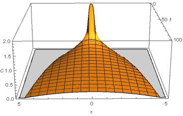
Figure 1: The concentration field $C(x,t)$ in (IV) for $\gamma=-1$ and $y_{c}=1$.

We may now reconstruct the normalized concentration field $C(x,t)$ using equation (14). We find

$$C(x,t) = \Theta\left(1-\left|\frac{x}{y_{c}t^{\frac{1}{2-\gamma}}}\right|\right)$$

$$\frac{1}{y_{c}t^{\frac{1}{2-\gamma}}}\ \frac{\Gamma\left[\frac{3}{2}-\frac{1}{\gamma}\right]}{\sqrt{\pi}\Gamma\left[1-\frac{1}{\gamma}\right]}\left[1-\left(\frac{x}{y_{c}t^{\frac{1}{2-\gamma}}}\right)^{2}\right]^{-\frac{1}{\gamma}}\;,$$

where $y_{c}=a\tilde{y}_{c}$. This is the solution that was found by Pattle p59 . We show it in figure 1 for $\gamma=-1$ and $y_{c}=1$.

We now calculate $x_{RMS}$ for $\gamma<0$. Hence,

$$x_{RMS}^{2}=\int_{-y_{c}t^{1/(2-\gamma)}}^{+y_{c}t^{1/(2-\gamma)}}dx\ x^{2}C(x,t)=\frac{-\gamma}{2-3\gamma}y_{c}t^{\frac{2}{2-\gamma}}\;,$$ (36)

where $C(x,t)$ is given by the solution (IV). By comparing with equation (1) we find equation (5) — as did Pattle.

V Solution for $0<\gamma<1$

We return to equation (25), now assuming that $K\neq 0$. We divide the equation by $|K|$ to get

$$\frac{c}{|K|}\ yp(y)+\frac{1}{|K|}\ \frac{d}{dy}p(y)^{1-\gamma}=\epsilon\;,$$ (37)

where

$$\epsilon=\frac{K}{|K|}=\pm 1\;.$$ (38)

This equation cannot be integrated directly as could the case for $K=0$. However, we will be able to pry the essential information from it anyway.

We non-dimensionalize equation (37) by invoking equations (27) and (28) and setting

$$\frac{c}{|K|}\ ab=1\;,$$ (39)

and

$$\frac{1}{|K|}\ \frac{b^{1-\gamma}}{a}=1\;.$$ (40)

Equation (37) thus becomes

$$\tilde{y}\tilde{p}(\tilde{y})+\frac{d}{d\tilde{y}}\tilde{p}(\tilde{y})^{1-\gamma}=\epsilon\;.$$ (41)

If $\epsilon=+1$, we must have from this equation that $d\tilde{p}(0)^{1-\gamma}/d\tilde{y}=1$ when $\tilde{y}=0$. A positive derivative at the origin means that $\tilde{p}(\tilde{y})$ increases as we move away from the origin. We may therefore discard this possibility as being unphysical. On the other hand, if $\epsilon=-1$, we must have that $d\tilde{p}(0)^{1-\gamma}/d\tilde{y}=-1$ when $\tilde{y}=0$, which makes physically sense. Hence, only the $\epsilon=-1$ case needs to be pursued further.

Suppose now that $\tilde{p}(\tilde{y})>0$ for all finite $\tilde{y}$. Since $C(x,t)$ is normalizable, we know that $\tilde{p}(\tilde{y})\to 0$ as $|\tilde{y}|\to\infty$ faster than $1/|\tilde{y}|$. Hence, $\tilde{y}\tilde{p}(\tilde{y})\to 0$ as $|\tilde{y}|\to\infty$. From equation (41) we then have that

$$\frac{d}{d\tilde{y}}\ \tilde{p}(\tilde{y})^{1-\gamma}\to-1\quad{\rm as}\ |\tilde{y}|\to\infty\;.$$ (42)

This is not possible, and we conclude that there is a finite $\tilde{y}_{c}$ such that $\tilde{p}(\tilde{y})=0$ for $|\tilde{y}|\geq\tilde{y}_{c}$.

We will in the following investigate how the solution of equation (41) behaves close to $\tilde{y}\approx 0$ and $\tilde{y}\approx\tilde{y}_{c}>0$. At $\tilde{y}=\tilde{y}_{c}$, equation (41) becomes

$$\frac{d}{d\tilde{y}}\ \tilde{p}(\tilde{y})^{1-\gamma}=-1\;.$$ (43)

We integrate this equation to find

$$\tilde{p}(\tilde{y})=(\tilde{y}_{c}-\tilde{y})^{\frac{1}{1-\gamma}}\;.$$ (44)

This is the lowest order expansion of $\tilde{p}$ around $\tilde{y}_{c}$. In order to find the next order, we assume $\tilde{p}$ to take the form

$$\tilde{p}(\tilde{y})^{1-\gamma}=(y_{c}-y)+\delta\tilde{p}(\tilde{y})\;.$$ (45)

We insert this expression into equation (41) and find that $\delta\tilde{p}(\tilde{y})$ obeys the equation

$$\tilde{y}_{c}(\tilde{y}_{c}-\tilde{y})^{\frac{1}{1-\gamma}}+\frac{d}{d\tilde{y}}\ \delta\tilde{p}(\tilde{y})=0\;.$$ (46)

We solve this equation and find

$$\delta\tilde{p}(\tilde{y})=\frac{1-\gamma}{2-\gamma}\tilde{y}_{c}(\tilde{y}_{c}-\tilde{y})^{\frac{2-\gamma}{1-\gamma}}\;.$$ (47)

Combining this result with equation (45) gives

$$\tilde{p}(\tilde{y})=\left(\tilde{y}_{c}-\tilde{y}\right)^{\frac{1}{1-\gamma}}\left[1+\frac{\tilde{y}_{c}}{2-\gamma}(\tilde{y}_{c}-\tilde{y})^{\frac{1}{1-\gamma}}+\cdots\right]\;.$$ (48)

We see from this expression that $d\tilde{p}(\tilde{y})/d\tilde{y}\to 0$ as $\tilde{y}\to\tilde{y}_{c}$, i.e., the profile approaches the maximum $\tilde{y}$ value with a slope that goes to zero. However, we have that

$$\frac{d^{2}\tilde{p}(\tilde{y})}{d\tilde{y}^{2}}=\frac{\gamma}{(1-\gamma)^{2}}(\tilde{y}_{c}-\tilde{y})^{\frac{2\gamma-1}{1-\gamma}}\;.$$ (49)

This expression is always positive and the $\tilde{p}(\tilde{y})$ profile is therefore always concave. However, we note that for $0<\gamma<1/2$, the second derivative diverges. Hence, the first derivative reaches zero in a ‘brutal’ way for these values of $\gamma$.

We now use equation (19) combined with the equations (47) and (48) to find

$$c=1\;,$$ (50)

to lowest order in $\tilde{y}_{c}-\tilde{y}$. Hence, $c>0$ and the solution for $\epsilon=-1$ is viable.

From equations (41) and (43), we have that

$$\frac{d}{d\tilde{y}}\ \tilde{p}(\tilde{y})^{1-\gamma}\to-1\quad{\rm as\ }\tilde{y}\to 0\ {\rm or\ }\tilde{y}\to\tilde{y}_{c}\;.$$ (51)

Hence, $\tilde{p}(\tilde{y})$ leaves the $\tilde{p}$ axis at $\tilde{y}=0$ with the same slope as it reaches the $\tilde{y}$ at $\tilde{y}_{c}$.

At $\tilde{y}=0$, we have that

$$\frac{d\tilde{p}(y)^{1-\gamma}}{d\tilde{y}}=-1\;$$ (52)

to lowest order in $\tilde{y}$. We integrate this expression and find

$$\tilde{p}(\tilde{y})^{1-\gamma}=\tilde{p}(0)^{1-\gamma}-\tilde{y}\;,$$ (53)

which to lowest order in $\tilde{y}$ gives

$$\tilde{p}(\tilde{y})=\tilde{p}(0)-\frac{\tilde{p}(0)^{\gamma}}{1-\gamma}\ y\;.$$ (54)

We see that $\tilde{p}(\tilde{y})$ approaches the $\tilde{y}=0$-axis at an angle. Hence, the maximum of the of the concentration profile forms a wedge.

Furthermore, for small $\tilde{y}>0$, we have that $d\tilde{y}\tilde{p}(\tilde{y})/d\tilde{y}=\tilde{p}(\tilde{y})+\tilde{y}d\tilde{p}(\tilde{y})/d\tilde{y}>0$ since we can make the second term in the middle as small as we wish by making $\tilde{y}$ small enough. Hence, we must have $d^{2}\ \tilde{p}(\tilde{y})^{1-\gamma}/d\tilde{y}^{2}<0$ to ensure $c>0$. This must be the case in order for the two terms on the left hand side in equation (24) to sum to zero. So, $\tilde{p}(\tilde{y})^{1-\gamma}$ must be convex near the origin. Since $1-\gamma<0$, $\tilde{p}(\tilde{y})$ must also be concave near $\tilde{y}=0$.

Near $\tilde{y}_{c}$, we have that

$$\frac{d}{d\tilde{y}}\ \tilde{y}\tilde{p}(\tilde{y})=-\frac{y_{c}}{1-\gamma}\ (\tilde{y}_{c}-\tilde{y})^{\frac{\gamma}{1-\gamma}}<0\;.$$ (55)

We furthermore find

$$\frac{d^{2}}{d\tilde{y}^{2}}\ \tilde{p}(\tilde{y})^{1-\gamma}=\frac{\tilde{y}_{c}}{1-\gamma}\ (\tilde{y}_{c}-\tilde{y})^{\frac{\gamma}{1-\gamma}}>0\;.$$ (56)

That is, $\tilde{p}(\tilde{y})^{1-\gamma}$ is concave near $\tilde{y}_{c}$. Since $1-\gamma<0$, $\tilde{p}(\tilde{y})$ must also be concave near $\tilde{y}_{c}$. Furthermore, we see that equation (56) diverges if $\gamma<0$ and it is well behaved if $\gamma>0$. Our conclusion is that the $\epsilon=-1$ solution corresponds to $\gamma>0$.

If we had the exact profile $\tilde{p}(\tilde{y})$, we could have proceeded to construct the normalized concentration field $C(x,t)$ as we did in equation (IV) for $\gamma<0$. We do not have this profile, but we may still conclude that equation (5) works also for $0<\gamma<1$, since

$$x_{RMS}^{2} = \int_{-y_{c}t^{1/(2-\gamma)}}^{+y_{c}t^{1/(2-\gamma)}}dx\ x^{2}C(x,t)$$ (57)

$$= \int_{-y_{c}t^{1/(2-\gamma)}}^{+y_{c}t^{1/(2-\gamma)}}dx\ \frac{x^{2}}{t^{\frac{1}{1-\gamma}}}p\left(\frac{x}{t^{\frac{1}{1-\gamma}}}\right)$$

$$\propto t^{\frac{2}{1-\gamma}}\;.$$

V.1 Does the $0<\gamma<1$ solution really exist?

When $0<\gamma<1$, the diffusivity given by equation (3) diverges. Still, the non-linear diffusion equation (4) is well behaved and has solutions, even if we are unable to write them down explicitly. We will in the following section model the diffusion processes described by (4) by a stochastic process involving diffusing particles. However, let us forego this discussion and already now picture the diffusion process described by (4) with $0<\gamma<1$. Focus on the region close to but to the left of the sharp front at $+\tilde{y}_{c}$. This region will be swarming with particles. There will always be a particles which is furthest to the right. This particle will be alone. Hence, according to the diverging diffusivity, this particle will be kicked off to $x\to\pm\infty$ and be gone. Then, there will be another particle furthest to the right which therefore will be alone, and the same happens to this one. And so on. Soon there will be no particles left.

This leakage is caused by fluctuations that are not described by the diffusion equation. In this case, they must dominate the process and they have a devastating effect on the solution of the non-linear diffusion equation we have just described. The solution to this dilemma is to add a small positive number $\delta$ to the concentration in this equation so that it becomes

$$D=D_{0}\left[C(x,t)+\delta\right]^{-\gamma}\;.$$ (58)

This changes the character of the diffusion equation when $C\approx\delta$, but it stops the “leakage” due to fluctuations. From a physical point of view, it makes sense that the the diffusion process goes normal for small enough concentrations. When $\delta$ is added in equation (58), the solution we have described here is still valid for $C>\delta$. We demonstrate this numerically in Section VI.4. Hence, the approach taken in this section is physically realistic.

VI Derivation of the diffusion equation from particle dynamics

We now turn to stochastic modeling of the process we so far have described using the non-linear diffusion equation (4).

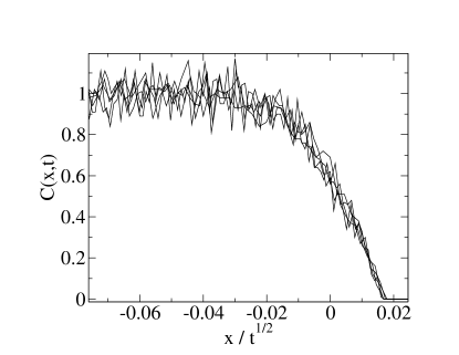
Figure 2: The concentration $C(x,t)$ as a function of $x/t^{1/2}$ when $\gamma=-1$ and the initial concentration was $C(x,0)=\Theta(-x)$, the Heaviside step function.

Following the discussion in the van Kampen book Stochastic Processes in Physics and Chemistry k07 , we derive the non-linear diffusion equation, which is an example of a Fokker-Planck equation from the following particle model: A population of $N_{p}$ particles are propagated by a sequence of random steps of zero mean using a concentration dependent step length. For every time the particle positions, which take on continuous values, are updated, the concentration field $C(x,t)$ is updated onto a discrete one-dimensional lattice of unit lattice constant. Their positions $x_{i}$ are updated according to the following algorithm

$$x\rightarrow x+\Delta x\;,$$ (59)

where

$$\Delta x=\eta g(C(x))\sqrt{\Delta t}$$ (60)

is a Wiener process and $\eta$ is a random variable with $\langle{\eta}\rangle=0$ and $\langle{\eta^{2}}\rangle=1$, where $g(C)$ may be the normalized concentration. Now, following the discussion in the van Kampen book, Chapter VIII.2 we derive the corresponding Fokker-Planck equation as follows. The Chapman-Kolmogorov or master equation describing the above stochastic process is

$$\frac{\partial C(x,t)}{\partial t}=\int_{-\infty}^{\infty}drC(x-r,t)W(x-r,r)-C(x,t)W(x,-r)\;,$$ (61)

where $W(x,r)$ is the number of particles per time and length that jump a distance $r$ starting from $x$. We note that the formalism remains valid also when $W(x,t)$ depends on $x$ via $c(x,t)$ itself. Taylor expanding the integrand around $x$ yields the Fokker-Planck equation

$$\frac{\partial C(x,t)}{\partial t}=\frac{1}{2}\frac{\partial^{2}}{\partial x^{2}}\left(a_{2}(x)C(x,t)\right)\;,$$ (62)

where $a_{2}(x)$ is the mean squared jump length per time,

$$a_{2}(x)=\int drr^{2}W(x,r)=\frac{\langle{\Delta x^{2}}\rangle}{\Delta t}=g(C)^{2}\;,$$ (63)

according to equation (60). Setting $g(C)=bC^{-\gamma/2}$ gives

$$\frac{\partial C}{\partial t}=\frac{b^{2}}{2}\frac{\partial^{2}}{\partial x^{2}}C^{1-\gamma}\;,$$ (64)

and requiring equivalence with equation (4) thus implies that $b^{2}=2/(1-\gamma)$.

VI.1 Itô-Stratonovitch dilemma

However, the presence of a $C$-dependence in the diffusivity $D$ introduces an ambiguity in the implementation of equation (59), since now $\Delta x$ also depends on $C$, which in turn depends on all the $\Delta x$’s. So, the question is whether one should use $C(x)$ or $C(x+\Delta x)$ or perhaps something in between? Since $\Delta x\sim\sqrt{\Delta t}$ these choices are not equivalent.

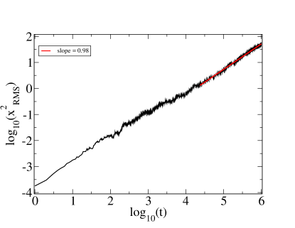
Figure 3: The mean square displacement as a function of time when $\gamma=-1$ and initial condition $C(x,0)=\Theta(-x)$, the Heaviside step function. According to the Boltzmann transformation, we expect $x_{RMS}\sim t^{1/2}$, which is precisely what we find.

Stratonovitch read equation (59) as k07

$$x\rightarrow x+g\left(\frac{c(x(t+\Delta t))+C(x(t))}{2}\right)\eta\sqrt{\Delta t}\;,$$ (65)

while Itô read it as

$$x\rightarrow x+g\left(C\left(x(t)\right)\right)\eta\sqrt{\Delta t}\;.$$ (66)

It turns out that it is the choice opted for by Itô that gives equation (62), while the Stratonovitch choice gives

$$\frac{\partial C}{\partial t}=\frac{1}{2}\frac{\partial}{\partial x}\left(g\frac{\partial}{\partial x}\left(gC\right)\right)\;,$$ (67)

see van Kampen’s book k07 , Chapter VI.4 for a derivation of this result. By setting $g(C)=bC^{-\gamma/2}$ again we can write the above equation as

$$\frac{\partial C}{\partial t}=\frac{b^{2}}{2}\frac{1-\gamma/2}{1-\gamma}\frac{\partial^{2}}{\partial x^{2}}C^{1-\gamma}\;,$$ (68)

and equivalence with equation (4) now implies that $b^{2}=2/(1-\gamma/2)$. This means that the only difference between the Itô and Stratonovitch implementations of equation (59) is the magnitude of the random step. In the Itô case the step length has to be a bit smaller than in the Stratonovitch case in order to correspond to the same macroscopic descriptions for $\gamma\neq 0$. When $\gamma=0$ the $C-$-dependence of $D$ goes away and the two interpretations give the same $b$, as one would expect.

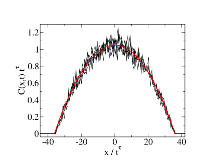
Figure 4: The scaled concentration $t^{\tau}C(x,t)$ as a function of $x/t^{\tau}$where $\tau=1/3$ according to equation (5) when $\gamma=-1$ and $dt=5\;10^{-5}$. The black lines show simulations at different times while the red shows a parabolic fit.

In the simulations it is convenient to use the Itô implementation and thus $\Delta x=\eta\sqrt{2\Delta t/(1-\gamma)}c^{-\gamma/2}$. First, the particles are initialized at the same location, so that the initial concentration is a $\delta$-function. The time step is $dt=5\;10^{-5}$ and $N_{p}=1000$ particles are used.

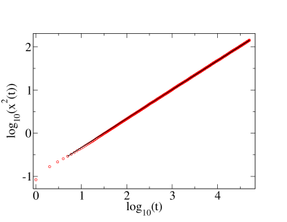
Figure 5: The mean square displacement as a function of time when $\gamma=-1$ so that $\tau=1/3$ according to equation (5). Hence, we expect $x_{RMS}\sim t^{2/3}$.

VI.2 The concentration is initially a step function

We start by considering the step initial conditions first studied by Boltzmann b94 . We start the simulations by setting $C(x,t=0)=\Theta(-x)$, where $\Theta(x)$ is the Heaviside step function, which is 0 for negative arguments and one for positive arguments. We show in figure 2 the concentration profile $C(x,t)$ for different times plotted against the reduced variable $y=x^{/}\sqrt{t}$, see equation (6) using $\gamma=-1$. There is data collapse in accordance with equation (8).

In figure 3 we show the RMS displacement $\sum_{i=1}^{N}x_{i}^{2}/N$ where the sum runs over all particles with positions $x_{i}>0$. This quantity is easily calculated as the motion of each particle is traced.

VI.3 Delta-function initialization: the $\gamma<0$ case

In this case we chose $\gamma=-1$. We had all the particles collected at the origin for $t=0$, thus fulfilling the initial condition (10). We then let the particles loose with the result shown in figure 4: $t^{\tau}C(x,t)$ plotted against $x/t^{\tau}$ where $\tau$ is given by equation (5), and hence equal to $1/3$. We have the exact solution for $C(x,t)$ for negative $\gamma$ given in equation (IV). When $\gamma=-1$, we expect a parabolic shape. We show this parabola in red in figure 4.

Figure 5 shows $x_{RMS}^{2}$ vs. $t$ on log-log scale. The straight line is a fit and we measure $\tau=0.67$ in comparison to the theoretical value $2\tau=2/3$, see equation (36).

VI.4 Delta-function initialization: the $0<\gamma<1$ case

Here we set $\gamma=1/2$. We use the regularized diffusivity given in equation (58) with $\delta=0.01$.

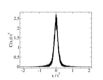
Figure 6: The scaled concentration $t^{\tau}C(x,t)$ as a function of $x/t^{\tau}$ when $\gamma=1/2$ so that $\tau=2/3$ according to equation (5).

We had as in the negative-$\gamma$ case all the particles collected at the origin for $t=0$, in accordance with the initial condition (10). The ensuing result is shown in figure 6: $t^{\tau}C(x,t)$ plotted against $x/t^{\tau}$ where $\tau$ is given by equation (5). In this case it is $2/3$. We do not have the analytical form of the profile in contrast to the negative $\gamma$ case.

Figure 7 shows $x_{RMS}^{2}$ vs. $t$ on log-log scale. The straight line is a fit and we measure $\tau=0.67$ in good comparison to the theoretical value $2\tau=4/3$.

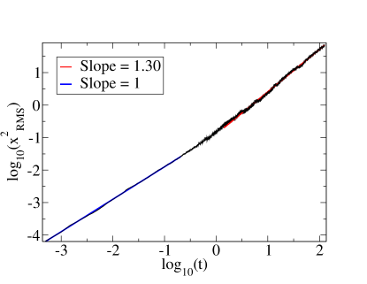
Figure 7: The mean square displacement as a function of time when $\gamma=1/2$ so that $\tau=2/3$ according to equation (5). Hence, we expect $x_{RMS}^{2}\sim t^{4/3}$. The black line is a fit with exponent $1.30$.

VI.5 Step-function initialization: the $0<\gamma<1$ case

As a test of the step function behavior for $\gamma>$0 we set $\gamma=3/4$ and initialize $N_{p}=$ 8000 particles at a constant density in a region $x\leq 0$. The results are shown in figures 8 where we plot $C(x,t)$ against both $x/t^{1/2}$ and $x/t^{\tau}$.

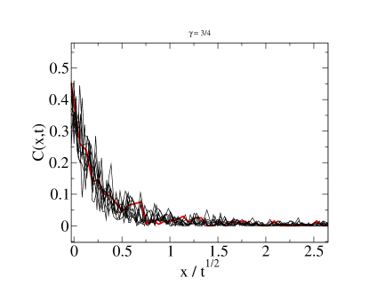
Figure 8: The evolution of the step profile when $\gamma=3/4$. We have plotted it as a function of position scaled by the two different factors $t^{\tau}$ where $\tau=4/5$ according to equation (5), and $t^{1/2}$. The first profile is red, the latter black.

It is seen that the data-collapse is somewhat better for the $x/t^{1/2}$ choice. Likewise, figure 9 shows a clear normal-diffusion scaling of $\langle{x^{2}}\rangle$.

Hence, also in the $0<\gamma<1$ case, we have that the step profile leads to normal diffusion.

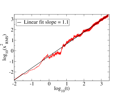
Figure 9: The mean square displacement $\int_{0}^{\infty}dxx^{2}C(x,t)/\int_{0}^{\infty}dxC(x,t)$ when $\gamma=3/4$.

We summarize our numerical findings in figure 10 where we compare the measured values of $\tau$ compared to the prediction in equation (5) over the range of $\gamma$-values $[-1,1]$, $\gamma=0$ excluded. As is apparent, the coincidence between the prediction (5) and the measured values are decreasingly matching as $\gamma$ approaches 1. There are two reasons for this, the first one being that the singularity in the diffusivity, equation (3), becomes more severe with increasing $\gamma$. The second reason is that the coupling between the master equation (61) and the Fokker-Planck equation (64) becomes increasingly tenuous as the expansion is done around a singular point.

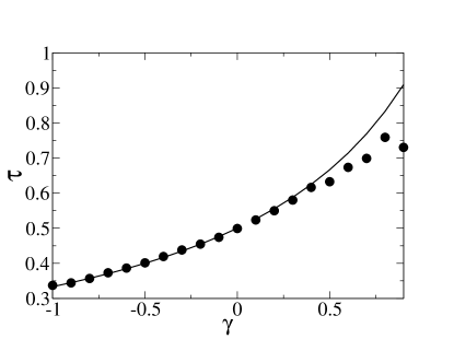
Figure 10: The measured diffusion exponent ($\bullet$) compared to the prediction of equation (5) (full line).

VII Summary and conclusions

A power law dependence of the diffusivity with respect to the concentration, equation (3) leads to anomalous diffusion. That is, the root-mean-square distance moved by a particle does not scale as the square root of time, but another power, see equation (1). The way to measure this quantity using the concentration field is to initialize the system with a delta function in the concentration. The result of Boltzmann b94 going back 125 years, is still surprising in light of this. When the concentration is initiated as a step function, the anomalous behavior seems to disappear: if we follow a given level of concentration $C(x(t),t)$ in time, we find $x(t)\sim\sqrt{t}$ in this case, as in normal diffusion.

With a power law diffusivity and a delta-function initial condition, there is no length scale in the problem. In this case normalizability leads to the scaling form of equation (22) leading to the exponent relation equation (5) which is the defining characteristic of anomalous diffusion. With a step function initial condition however, the solution extends to $x=-\infty$ and cannot any more by normalized. Hence, in this case, equation (22) is replaced by equation (8) which gives normal $\tau=1/2$ diffusion. If the step function were modified to a normalizable profile, it would necessarily imply the introduction of a length scale.

We have in this paper reviewed the Boltzmann result and demonstrated, as did Pattle 60 years ago p59 , that when $D(C)\sim C^{-\gamma}$ where $\gamma<0$, the non-linear diffusion equation is analytically solvable and indeed leads to anomalous diffusion. We go on, however, to consider the case when $0<\gamma<1$ which is not analytically solvable. Also this case shows anomalous diffusion, and we work this out analytically even though we are not able to solve for the entire concentration profile.

We then go on to construct a stochastic particle dynamics that we implement computationally. Using this approach, we are able to verify the central results we have derived earlier. They all match.

A couple of remarks at the very end:

Küntz and Lavallée kl04 conclude their abstract of their paper with the words ‘Spreading fronts are subdiffusive for $D(C)$ decreasing with $C$, superdiffusive for increasing $D(C)$ and scale only as $t^{1/2}$ only for constant $D$.’ Our findings here are the opposite. We find superdiffusive behavior when $<0\gamma<1$, i.e., $D(C)$ decreasing with increasing $C$ and we find subdiffusive behavior when $\gamma<0$, i.e., $D(C)$ increasing with increasing $C$. However, if we compare figures 4 and 6 where we plot $t^{\tau}C(x,t)$ against $x/t^{\tau}$ for $\gamma=-1<0$ and for $\gamma=1/2>0$, we see that the former curve ($\gamma<0$) which is a parabola, is ‘fatter’ than the latter curve ($\gamma>0$), which gives the appearance of a ‘skinny’ bell curve. Hence, relatively rather than in absolute terms, the $\gamma<0$ case propagates the walkers further away from the origin than the $\gamma>0$. In this sense, we agree with Küntz and Lavallée.

We mentioned in the introduction, anomalous diffusion originating from a concentration dependent diffusivity may have been seen in diffusion in granular media ffas09 ; cs12 . These observations are based on rotating a bi-disperse composition of smaller and large glass beads in a horizontal cylindrical mixer. The mixer is filled with the larger beads except for a small disk of smaller beads. As the cylinder turns, the smaller beads diffuse into the larger beads and the concentration of smaller beads as a function of time and position along the cylinder is recorded. This setup mimics closely the initial conditions that we have studied here, except for Section II, where we assumed a step initially. The connection with the present work is the proposal that the diffusivity of the smaller beads is larger when they are surrounded by other smaller beads than when they are surrounded by the larger beads; the higher the concentration of smaller beads, the larger their diffusivity is. We propose here to prepare the packing in a different way initially. Fill (say) the left half of the cylinder with the smaller beads and the right half with the larger beads. The system is therefore initiated with a step function in the concentration. According to Boltzmann, as demonstrated in Section II, one would then expect normal diffusion where the front evolves as $x^{2}\sim t$, i.e., the parabolic law.

- (1) L. Boltzmann, Zur Integration der Diffusionsgleichung bei variabeln Diffusionscoefficienten, Ann. der Physik, 289, 959–964 (1894); doi.org/10.1002/andp.18942891315.
- (2) J. Crank, The Mathematics of Diffusion (Oxford University Press, Oxford, 1975).
- (3) R. Metzler and J. Klafter, The random walk’s guide to anomalous diffusion: a fractional dynamics approach, Phys. Rep. 339, 1-77 (2000); doi.org/10.1016/S0370-1573(00)00070-3.
- (4) W. I. Newman, Some exact solutions to a non-linear diffusion problem in population genetics and combustion, J. Theor. Biology, 85, 325–334 (1980); doi.org/10.1016/0022-5193(80)90024-7.
- (5) E. N. de Azevedo, P. L. de Sousa, R. E. de Souza, M. Engelsberg, M. de N. do N. Miranda, and M. A. Silva, Concentration-dependent diffusivity and anomalous diffusion: A magnetic resonance imaging study of water ingress in porous zeolite, Phys. Rev. E, 73, 011204 (2006); doi.org/10.1103/PhysRevE.73.011204.
- (6) E. N. de Azevedo, D. V. da Silva, R. E. de Souza, and M. Engelsberg, Water ingress in Y-type zeolite: Anomalous moisture-dependent transport diffusivity, Phys. Rev. E, 74, 041108 (2006); doi.org/10.1103/PhysRevE.74.041108.
- (7) D. Fischer, T. Finger, F. Angenstein and R. Stannarius, Diffusive and subdiffusive axial transport of granular material in rotating mixers, Phys. Rev. E, 80, 061302 (2009); doi.org/10.1103/PhysRevE.80.061302.
- (8) I. C. Christov and H. A. Stone, Resolving a paradox of anomalous scalings in the diffusion of granular materials, Proc. Natl. Acad. Science, 109, 16012–16017 (2012); doi.org/10.1073/pnas.1211110109.
- (9) A. Hansen, B. S. Skagerstam and G. Tørå, Anomalous Scaling and Solitary Waves in Systems with Non-Linear Diffusion, Phys. Rev. E, 83, 056314 (2011); doi.org/10.1103/PhysRevE.83.056314.
- (10) M. Küntz and P. Lavallée, Anomalous diffusion is the rule in concentration-dependent diffusion processes, J. Phys. D: Appl. Phys. 37, L5–L8 (2004); doi.org/10.1088/0022-3727/37/1/L02.
- (11) R. E. Pattle, Diffusion from an instantaneous point source with a concentration-dependent coefficient, Q. Mechanics Appl. Math. 12, 407–409 (1959); doi.org/10.1093/qjmam/12.4.407.
- (12) N. G. van Kampen, Stochastic Processes in Physics and Chemistry, 3rd Edition (North-Holland, Amsterdam, 2007).