Bayesian Variational Autoencoders for
Unsupervised Out-of-Distribution Detection

Abstract

Despite their successes, deep neural networks may make unreliable predictions when faced with test data drawn from a distribution different to that of the training data, constituting a major problem for AI safety. While this has recently motivated the development of methods to detect such out-of-distribution (OoD) inputs, a robust solution is still lacking. We propose a new probabilistic, unsupervised approach to this problem based on a Bayesian variational autoencoder model, which estimates a full posterior distribution over the decoder parameters using stochastic gradient Markov chain Monte Carlo, instead of fitting a point estimate. We describe how information-theoretic measures based on this posterior can then be used to detect OoD inputs both in input space and in the model’s latent space. We empirically demonstrate the effectiveness of our proposed approach.

1 Introduction

Outlier detection in input space. While deep neural networks (DNNs) have successfully tackled complex real-world problems in various domains including vision, speech and language [39], they still face significant limitations that make them unfit for safety-critical applications [5]. One well-known shortcoming of DNNs is when faced with test data points coming from a different distribution than the data the network saw during training, the DNN will not only output incorrect predictions, but it will do so with high confidence [52]. The lack of robustness of DNNs to such out-of-distribution (OoD) inputs (or outliers/anomalies) was recently addressed by various methods to detect OoD inputs in the context of prediction tasks (typically classification) [28, 40, 29]. When we are only given input data, one simple and seemingly sensible approach to detect a potential OoD input ${\mathbf{x}}^{*}$ is to train a likelihood-based deep generative model (DGM; e.g. a VAE, auto-regressive DGM, or flow-based DGM) by (approximately) maximizing the probability $p({\mathbb{D}}|\theta)$ of the training data ${\mathbb{D}}$ under the model parameters $\theta$, and to then estimate the density $p({\mathbf{x}}^{*}|\theta)$ of ${\mathbf{x}}^{*}$ under the generative model $\theta$ [9]. If $p({\mathbf{x}}^{*}|\theta)$ is large, then ${\mathbf{x}}^{*}$ is likely in-distribution, and OoD otherwise. However, recent works have shown that this likelihood-based approach does not work in general, as DGMs sometimes assign higher density to OoD data than to in-distribution data [49]. While some papers developed more effective scores that correct the likelihood [14, 58, 50], we argue and show that OoD detection methods fundamentally based on the unreliable likelihood estimates by DGMs are not robust.

Outlier detection in latent space. In a distinct line of research, recent works have tackled the challenge of optimizing a costly-to-evaluate black-box function $f:{\mathbb{X}}\rightarrow{\mathbb{R}},f({\mathbf{x}})=y$ over a high-dimensional, richly structured input domain ${\mathbb{X}}$ (e.g. graphs, images). Given data ${\mathbb{D}}=\{({\mathbf{x}}_{i},y_{i})\}_{i=1}^{N}$, these methods jointly train a VAE on inputs ${\mathbf{x}}$ and a predictive model $g:{\mathbb{Z}}\rightarrow{\mathbb{R}},g({\mathbf{z}})=y$ mapping from latent codes ${\mathbf{z}}$ to targets $y$, to then perform the optimization w.r.t. $y$ in the low-dimensional, continuous latent space ${\mathbb{Z}}$ instead of in input space ${\mathbb{X}}$ [22]. While these methods have achieved strong results in domains including automatic chemical design and automatic machine learning [22, 42, 41, 67], their practical effectiveness is limited by their ability to handle the following trade-off: They need to find inputs ${\mathbf{x}}$ that both have a high target value $y$ and are sufficiently novel (i.e., not too close to training inputs ${\mathbb{D}}$), and at the same time ensure that the optimization w.r.t. $y$ does not progress into regions of the latent space ${\mathbb{Z}}$ too far away from the training data, which might yield latent points ${\mathbf{z}}$ that decode to semantically meaningless or syntactically invalid inputs ${\mathbf{x}}$ [37]. The required ability to quantify the novelty of latents ${\mathbf{z}}$ (i.e., the semantic/syntactic distance to ${\mathbb{D}}$) directly corresponds to the ability to effectively detect outliers in latent space ${\mathbb{Z}}$.

Our approach. We propose a novel unsupervised, probabilistic method to simultaneously tackle the challenge of detecting outliers ${\mathbf{x}}^{*}$ in input space ${\mathbb{X}}$ as well as outliers ${\mathbf{z}}^{*}$ in latent space ${\mathbb{Z}}$. To this end, we take an information-theoretic perspective on OoD detection, and propose to use the (expected) informativeness of an input ${\mathbf{x}}^{*}$ / latent ${\mathbf{z}}^{*}$ as a proxy for whether ${\mathbf{x}}^{*}$ / ${\mathbf{z}}^{*}$ is OoD or not. To quantify this informativeness, we leverage probabilistic inference methods to maintain a posterior distribution over the parameters of a DGM, in particular of a variational autoencoder (VAE) [36, 59]. This results in a Bayesian VAE (BVAE) model, where instead of fitting a point estimate of the decoder parameters via maximum likelihood, we estimate their posterior using samples generated via stochastic gradient Markov chain Monte Carlo (MCMC). The informativeness of an unobserved ${\mathbf{x}}^{*}$ / ${\mathbf{z}}^{*}$ is then quantified by measuring the (expected) change in the posterior over model parameters after having observed ${\mathbf{x}}^{*}$ / ${\mathbf{z}}^{*}$, revealing an intriguing connection to information-theoretic active learning [43].

Our contributions. (a) We explain how DGMs can be made more robust by capturing epistemic uncertainty via a posterior distribution over their parameters, and describe how such Bayesian DGMs can effectively detect outliers both in input space and in the model’s latent space based on information-theoretic principles (Section 3). (b) We propose a Bayesian VAE model as a concrete instantiation of a Bayesian DGM (Section 4). (c) We empirically demonstrate that our approach significantly outperforms previous OoD detection methods across commonly-used benchmarks (Section 5).

2 Problem Statement and Background

2.1 Out-of-Distribution (OoD) Detection

For input space OoD detection, we are given a large set ${\mathbb{D}}=\{{\mathbf{x}}_{i}\}_{i=1}^{N}$ of high-dimensional training inputs ${\mathbf{x}}_{i}\in{\mathbb{X}}$ (i.e., with $N>25,000$ and $\text{dim}({\mathbb{X}})>500$) drawn i.i.d. from a distribution $p^{*}({\mathbf{x}})$, and a single test input ${\mathbf{x}}^{*}$, and need to determine if ${\mathbf{x}}^{*}$ was drawn from $p^{*}$ or from some other distribution $\tilde{p}\neq p^{*}$. Latent space OoD detection is analogous, but with an often smaller set of typically lower-dimensional latent points ${\mathbf{z}}_{i}\in{\mathbb{Z}}$ (i.e., with $\text{dim}({\mathbb{Z}})<100$).

2.2 Variational Autoencoders

Consider a latent variable model $p({\mathbf{x}},{\mathbf{z}}|\theta)$ with marginal log-likelihood (or evidence) $\log p({\mathbf{x}}|\theta)=\log\int p({\mathbf{x}},{\mathbf{z}}|\theta)d{\mathbf{z}}$, where ${\mathbf{x}}$ are observed variables, ${\mathbf{z}}$ are latent variables, and $\theta$ are model parameters. We assume that $p({\mathbf{x}},{\mathbf{z}}|\theta)=p({\mathbf{x}}|{\mathbf{z}},\theta)p({\mathbf{z}})$ factorizes into a prior distribution $p({\mathbf{z}})$ over ${\mathbf{z}}$ and a likelihood $p({\mathbf{x}}|{\mathbf{z}},\theta)$ of ${\mathbf{x}}$ given ${\mathbf{z}}$ and $\theta$. As we assume the ${\mathbf{z}}$ to be continuous, $p({\mathbf{x}}|\theta)$ is intractable to compute. We obtain a variational autoencoder (VAE) [36, 59] if $\theta$ are the parameters of a DNN (the decoder), and the resulting intractable posterior $p({\mathbf{z}}|{\mathbf{x}},\theta)$ over ${\mathbf{z}}$ is approximated using amortized variational inference (VI) via another DNN $q({\mathbf{z}}|{\mathbf{x}},\phi)$ with parameters $\phi$ (the encoder or inference/recognition network). Given training data ${\mathbb{D}}$, the parameters $\theta$ and $\phi$ of a VAE are learned by maximizing the evidence lower bound (ELBO) $\sum_{{\mathbf{x}}\in{\mathbb{D}}}\mathcal{L}_{\theta,\phi}({\mathbf{x}})$, where

$${\mathcal{L}}_{\theta,\phi}({\mathbf{x}})=\mathbb{E}_{q({\mathbf{z}}|{\mathbf{x}},\phi)}[\log p({\mathbf{x}}|{\mathbf{z}},\theta)]-\text{KL}[{q({\mathbf{z}}|{\mathbf{x}},\phi)}\|p({\mathbf{z}})]$$ (1)

for ${\mathbf{x}}\in{\mathbb{D}}$, with ${\mathcal{L}}_{\theta,\phi}({\mathbf{x}})\leq\log p({\mathbf{x}}|\theta)$. As maximizing the ELBO approximately maximizes the evidence $\log p({\mathbb{D}}|\theta)$, this can be viewed as approximate maximum likelihood estimation (MLE). In practice, ${\mathcal{L}}_{\theta,\phi}({\mathbf{x}})$ in Eq. 1 is optimized by mini-batch stochastic gradient-based methods using low-variance, unbiased, stochastic Monte Carlo estimators of $\nabla\mathcal{L}_{\theta,\phi}$ obtained via the reparametrization trick. Finally, one can use importance sampling w.r.t. the variational posterior $q({\mathbf{z}}|{\mathbf{x}},\phi)$ to get an estimator $\hat{p}({\mathbf{x}}|\theta,\phi)$ of the probability $p({\mathbf{x}}|\theta)$ of an input ${\mathbf{x}}$ under the generative model, i.e.,

$$p({\mathbf{x}}|\theta)\simeq\hat{p}({\mathbf{x}}|\theta,\phi)=\textstyle\frac{1}{K}\textstyle\sum_{k=1}^{K}\frac{p({\mathbf{x}}|{\mathbf{z}}_{k},\theta)p({\mathbf{z}}_{k})}{q({\mathbf{z}}_{k}|{\mathbf{x}},\phi)}\ ,$$ (2)

where ${\mathbf{z}}_{k}\sim q({\mathbf{z}}|{\mathbf{x}},\phi)$ and where the estimator $\hat{p}({\mathbf{x}}|\theta,\phi)$ is conditioned on both $\theta$ and $\phi$ to make explicit the dependence on the parameters $\phi$ of the proposal distribution $q({\mathbf{z}}|{\mathbf{x}},\phi)$.

3 Information-theoretic Out-of-Distribution Detection

3.1 Motivation and Intuition

Why do deep generative models fail at OoD detection? Consider the approach which first trains a density estimator parameterized by $\theta$, and then classifies an input ${\mathbf{x}}^{*}$ as OoD based on a threshold on the density of ${\mathbf{x}}^{*}$, i.e., if $p({\mathbf{x}}^{*}|\theta)<\tau$ [9]. Recent advances in deep generative modeling (DGM) allow us to do density estimation even over high-dimensional, structured input domains (e.g. images, text), which in principle enables us to use this method in such complex settings. However, the resulting OoD detection performance fundamentally relies on the quality of the likelihood estimates produced by these DGMs. In particular, a sensible density estimator should assign high density to everything within the training data distribution, and low density to everything outside – a property of crucial importance for effective OoD detection. Unfortunately, [49, 14] found that modern DGMs are often poorly calibrated, assigning higher density to OoD data than to in-distribution data. This questions the use of DGMs for reliable density estimation and thus robust OoD detection.

How are deep discriminative models made OoD robust? DNNs are typically trained by maximizing the likelihood $p({\mathbb{D}}|\theta)$ of a set of training examples ${\mathbb{D}}$ under model parameters $\theta$, yielding the maximum likelihood estimate (MLE) $\theta^{*}$ [24]. For discriminative, predictive models $p(y|{\mathbf{x}},\theta)$, it is well known that the point estimate $\theta^{*}$ does not capture model / epistemic uncertainty, i.e., uncertainty about the choice of model parameters $\theta$ induced by the fact that many different models $\theta$ might have generated ${\mathbb{D}}$. As a result, discriminative models $p(y|{\mathbf{x}},\theta^{*})$ trained via MLE tend to be overconfident in their predictions, especially on OoD data [52, 27]. A principled, established way to capture model uncertainty in DNNs is to be Bayesian and infer a full distribution $p(\theta|{\mathbb{D}})$ over parameters $\theta$, yielding the predictive distribution $p(y|{\mathbf{x}},{\mathbb{D}})=\int p(y|{\mathbf{x}},\theta)p(\theta|{\mathbb{D}})d\theta$ [20]. Bayesian DNNs have much better OoD robustness than deterministic ones (e.g., producing low uncertainty for in-distribution and high uncertainty for OoD data), and OoD calibration has become a major benchmark for Bayesian DNNs [21, 56, 55, 44]. This suggests that capturing model uncertainty via Bayesian inference is a promising way to achieve robust, principled OoD detection.

Why should we use Bayesian DGMs for OoD detection? Just like deep discriminative models, DGMs are typically trained by maximizing the probability $p({\mathbb{D}}|\theta)$ that ${\mathbb{D}}$ was generated by the density model, yielding the MLE $\theta^{*}$. As a result, it is not surprising that the shortcomings of MLE-trained discriminative models also translate to MLE-trained generative models, such as the miscalibration and unreliability of their likelihood estimates $p({\mathbf{x}}^{*}|\theta^{*})$ for OoD inputs ${\mathbf{x}}^{*}$. This is because there will always be many different plausible generative / density models $\theta$ of the training data ${\mathbb{D}}$, which are not captured by the point estimate $\theta^{*}$. If we do not trust our predictive models $p(y|{\mathbf{x}},\theta^{*})$ on OoD data, why should we trust our generative models $p({\mathbf{x}}|\theta^{*})$, given that both are based on the same, unreliable DNNs? In analogy to the discriminative setting, we argue that OoD robustness can be achieved by capturing the epistemic uncertainty in the DGM parameters $\theta$. This motivates the use of Bayesian DGMs, which estimate a full distribution $p(\theta|{\mathbb{D}})$ over parameters $\theta$ and thus capture many different density estimators to explain the data, yielding the expected/average likelihood

$$p({\mathbf{x}}|{\mathbb{D}})=\textstyle\int p({\mathbf{x}}|\theta)p(\theta|{\mathbb{D}})d\theta=\mathbb{E}_{p(\theta|{\mathbb{D}})}[p({\mathbf{x}}|\theta)]\ .$$ (3)

How can we use Bayesian DGMs for OoD detection? Assume that given data ${\mathbb{D}}$, we have inferred a distribution $p(\theta|{\mathbb{D}})$ over the parameters $\theta$ of a DGM. In particular, we consider the case where $p(\theta|{\mathbb{D}})$ is represented by a set $\{\theta_{m}\}_{m=1}^{M}$ of $M$ samples $\theta_{m}\sim p(\theta|{\mathbb{D}})$, which can be viewed as an ensemble of $M$ DGMs. Our goal now is to decide if a given, new input ${\mathbf{x}}^{*}$ is in-distribution or OoD. To this end, we refrain from classifying ${\mathbf{x}}^{*}$ as OoD based on a threshold on the (miscalibrated) likelihoods that one or more of the models $\{\theta_{m}\}_{m=1}^{M}$ assign to ${\mathbf{x}}^{*}$ [9]. Instead, we propose to use a threshold on a measure $D[\cdot]$ of the variation or disagreement in the likelihoods $\{p({\mathbf{x}}^{*}|\theta_{m})\}_{m=1}^{M}$ of the different models $\{\theta_{m}\}_{m=1}^{M}$, i.e., to classify an input ${\mathbf{x}}^{*}$ as OoD if $D[\{p({\mathbf{x}}^{*}|\theta_{m})\}_{m=1}^{M}]<\tau$. In particular, if the models $\{\theta_{m}\}_{m=1}^{M}$ agree as to how probable ${\mathbf{x}}^{*}$ is, then ${\mathbf{x}}^{*}$ likely is an in-distribution input. Conversely, if the models $\{\theta_{m}\}_{m=1}^{M}$ disagree as to how probable ${\mathbf{x}}^{*}$ is, then ${\mathbf{x}}^{*}$ likely is an OoD input. This intuitive decision rule is a direct consequence of the property that the epistemic uncertainty of a parametric model $\theta$ (which is exactly what the variation/disagreement across models $\{\theta_{m}\}_{m=1}^{M}$ captures) is naturally low for in-distribution and high for OoD inputs – the very same property that makes Bayesian discriminative DNNs robust to OoD inputs.

3.2 Quantifying Disagreement between Models

We propose the following score $D_{\Theta}[{\mathbf{x}}^{*}]$ to quantify the disagreement or variation in the likelihoods $\{p({\mathbf{x}}^{*}|\theta_{m})\}_{m=1}^{M}$ of a set $\{\theta_{m}\}_{m=1}^{M}$ of model parameter samples $\theta_{m}\sim p(\theta|{\mathbb{D}})$:

$$D_{\Theta}[{\mathbf{x}}^{*}]=\textstyle\frac{1}{\sum_{\theta\in\Theta}w_{\theta}^{2}},\quad\text{with}\quad w_{\theta}=\textstyle\frac{p({\mathbf{x}}^{*}|\theta)}{\sum_{\theta\in\Theta}p({\mathbf{x}}^{*}|\theta)}\ .$$ (4)

I.e., the likelihoods $\{p({\mathbf{x}}^{*}|\theta_{m})\}_{m=1}^{M}$ are first normalized to yield $\{w_{\theta_{m}}\}_{m=1}^{M}$ (see Eq. 4), such that $w_{\theta}\in[0,1]$ and $\sum_{\theta\in\Theta}w_{\theta}=1$. The normalized likelihoods $\{w_{\theta_{m}}\}_{m=1}^{M}$ effectively define a categorical distribution over models $\{\theta_{m}\}_{m=1}^{M}$, where each value $w_{\theta}$ can be interpreted as the probability that ${\mathbf{x}}^{*}$ was generated from the model $\theta$, thus measuring how well ${\mathbf{x}}^{*}$ is explained by the model $\theta$, relative to the other models. To obtain the score $D_{\Theta}[{\mathbf{x}}^{*}]$ in Eq. 4, we then square the normalized likelihoods, sum them up, and take the reciprocal. Note that $D_{\Theta}[{\mathbf{x}}^{*}]\in[1,M],\forall{\mathbf{x}}^{*}$.For latent points ${\mathbf{z}}^{*}\in{\mathbb{Z}}$, we take into account all possible inputs ${\mathbf{x}}^{*}\in{\mathbb{X}}$ corresponding to ${\mathbf{z}}^{*}$, yielding the expected disagreement $D_{\Theta}[{\mathbf{z}}^{*}]=\mathbb{E}_{p({\mathbf{x}}|{\mathbf{z}}^{*})}\left[D_{\Theta}[{\mathbf{x}}]\right]\simeq\textstyle\frac{1}{N}\textstyle\sum_{n=1}^{N}D_{\Theta}[{\mathbf{x}}_{n}]$, with inputs ${\mathbf{x}}_{n}$ sampled from the conditional distribution $p({\mathbf{x}}|{\mathbf{z}}^{*})$, and $D_{\Theta}[{\mathbf{x}}]$ defined as in Eq. 4.

As $D_{\Theta}[\cdot]$ measures the degree of disagreement between the models $\{\theta_{m}\}_{m=1}^{M}$ as to how probable ${\mathbf{x}}^{*}$/${\mathbf{z}}^{*}$ is, it can be used to classify ${\mathbf{x}}^{*}$/${\mathbf{z}}^{*}$ as follows: If $D_{\Theta}[\cdot]$ is large, then $[w_{\theta}]_{\theta\in\Theta}$ is close to the (discrete) uniform distribution $[\frac{1}{M}]_{\theta\in\Theta}$ (for which $D_{\Theta}[\cdot]=M$), meaning that all models $\theta\in\Theta$ explain ${\mathbf{x}}^{*}$/${\mathbf{z}}^{*}$ equally well and are in agreement as to how probable ${\mathbf{x}}^{*}$/${\mathbf{z}}^{*}$ is. Thus, ${\mathbf{x}}^{*}$/${\mathbf{z}}^{*}$ likely is in-distribution. Conversely, if $D_{\Theta}[\cdot]$ is small, then $[w_{\theta}]_{\theta\in\Theta}$ contains a few large weights (i.e., corresponding to models that by chance happen to explain ${\mathbf{x}}^{*}$/${\mathbf{z}}^{*}$ well), with all other weights being very small, where in the extreme case, $[w_{\theta}]_{\theta\in\Theta}=[0,\ldots,0,1,0,\ldots,0]$ (for which $D_{\Theta}[\cdot]=1$). This means that the models do not agree as to how probable ${\mathbf{x}}^{*}$/${\mathbf{z}}^{*}$ is, so that ${\mathbf{x}}^{*}$/${\mathbf{z}}^{*}$ likely is OoD.

As we argue in more detail in Appendix B, there is a principled justification for the disagreement score $D_{\Theta}[{\mathbf{x}}^{*}]$ in Eq. 4, which induces an information-theoretic perspective on OoD detection. In particular, $D_{\Theta}[{\mathbf{x}}^{*}]$ can be viewed as quantifying the informativeness of ${\mathbf{x}}^{*}$ for updating the DGM parameters $\theta$ to the ones capturing the true density. The OoD detection mechanism described above can thus be intuitively summarised as follows: In-distribution inputs ${\mathbf{x}}^{*}$ are similar to the data points already in ${\mathbb{D}}$ and thus uninformative about the model parameters $\theta$, inducing small change in the posterior distribution $p(\theta|{\mathbb{D}})$, resulting in a large score $D_{\Theta}[{\mathbf{x}}^{*}]$. Conversely, OoD inputs ${\mathbf{x}}^{*}$ are very different from the previous observations in ${\mathbb{D}}$ and thus informative about the model parameters $\theta$, inducing large change in the posterior $p(\theta|{\mathbb{D}})$, resulting in a small score $D_{\Theta}[{\mathbf{x}}^{*}]$. This perspective on OoD detection reveals a close relationship to information-theoretic active learning [43, 31]. There, the same notion of informativeness (or, equivalently, disagreement) is used to quantify the novelty of an input ${\mathbf{x}}^{*}$ to be added to the data ${\mathbb{D}}$, aiming to maximally improve the estimate of the model parameters $\theta$ by maximally reducing the entropy / epistemic uncertainty in the posterior $p(\theta|{\mathbb{D}})$.

4 The Bayesian Variational Autoencoder (BVAE)

As an example of a Bayesian DGM, we propose a Bayesian VAE (BVAE), where instead of fitting the model parameters $\theta$ via (approximate) MLE, $\theta_{\text{MLE}}=\operatorname{arg\,max}_{\theta}{\mathcal{L}}_{\theta,\phi}({\mathbb{D}})$, to get the likelihood $p({\mathbf{x}}|{\mathbf{z}},\theta_{\text{MLE}})$, we place a prior $p(\theta)$ over $\theta$ and estimate its posterior $p(\theta|{\mathbb{D}})\propto p({\mathbb{D}}|\theta)p(\theta)$, yielding the likelihood $p({\mathbf{x}}|{\mathbf{z}},{\mathbb{D}})=\int p({\mathbf{x}}|{\mathbf{z}},\theta)p(\theta|{\mathbb{D}})d\theta$. The marginal likelihood $p({\mathbf{x}}|{\mathbb{D}})=\textstyle\int\textstyle\int p({\mathbf{x}}|{\mathbf{z}},\theta)p({\mathbf{z}})d{\mathbf{z}}p(\theta|{\mathbb{D}})d\theta$ thus integrates out both the latent variables ${\mathbf{z}}$ and model parameters $\theta$ (cf. Eq. 3). The resulting generative process draws a ${\mathbf{z}}\sim p({\mathbf{z}})$ from its prior and a $\theta\sim p(\theta|{\mathbb{D}})$ from its posterior, and then generates ${\mathbf{x}}\sim p({\mathbf{x}}|{\mathbf{z}},\theta)$.Training a BVAE thus requires Bayesian inference of both the posterior $p({\mathbf{z}}|{\mathbf{x}},{\mathbb{D}})$ over ${\mathbf{z}}$ and the posterior $p(\theta|{\mathbb{D}})$ over $\theta$, which is both intractable and thus requires approximation. We propose two variants for inferring those posteriors in a BVAE.

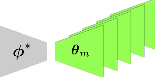
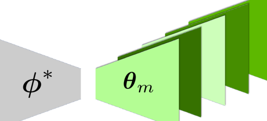
(a) Variant 1 with a shared encoder $\phi^{*}$ and $M$ decoders

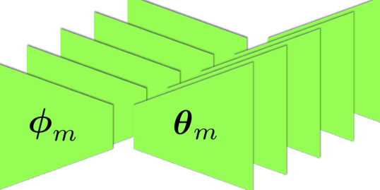
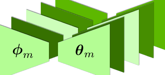
(b) Variant 2 as an ensemble of $M$ VAEs $(\phi_{m},\theta_{m})$

Figure 1: Illustrations of the (a) first and (b) second BVAE variant (with $M=5$), with (left) agreement and (right) disagreement in their likelihoods $p({\mathbf{x}}^{*}|\theta_{m})$ (as encoded by color intensity).

4.1 Variant 1: BVAE with a Single Fixed Encoder

a) Learning the encoder parameters $\phi$. As in a regular VAE, we approximate the posterior $p({\mathbf{z}}|{\mathbf{x}},{\mathbb{D}})$ using amortized VI via an inference network $q({\mathbf{z}}|{\mathbf{x}},\phi)$ whose parameters $\phi$ are fit by maximizing the ELBO ${\mathcal{L}}_{\theta,\phi}({\mathbf{x}})$ in Eq. 1, $\phi^{*}=\operatorname{arg\ max}{\mathcal{L}}_{\theta,\phi}({\mathbf{x}})$, yielding a single fixed encoder.

b) Learning the decoder parameters $\theta$. To generate posterior samples $\theta\sim p(\theta|{\mathbb{D}})$ of decoder parameters, we propose to use SGHMC (see Appendix A). However, the gradient of the energy function $\nabla_{\theta}U(\theta,{\mathbb{M}})$ in Eq. 5 used for simulating the Hamiltonian dynamics requires evaluating the log-likelihood $\log p({\mathbf{x}}|\theta)$, which is intractable in a (B)VAE. To alleviate this, we approximate the log-likelihood in $\nabla_{\theta}U(\theta,{\mathbb{M}})$ by the ordinary VAE ELBO ${\mathcal{L}}_{\theta,\phi}({\mathbf{x}})$ in Eq. 1. Given a set $\Theta=\{\theta_{m}\}_{m=1}^{M}$ of posterior samples $\theta_{m}\sim p(\theta|{\mathbb{D}})$, we can more intuitively think of having a finite mixture/ensemble of decoders/generative models $p({\mathbf{x}}|{\mathbf{z}},{\mathbb{D}})=\mathbb{E}_{p(\theta|{\mathbb{D}})}[p({\mathbf{x}}|{\mathbf{z}},\theta)]\simeq\frac{1}{M}\sum_{\theta\in\Theta}p({\mathbf{x}}|{\mathbf{z}},\theta)$.

c) Likelihood estimation. This BVAE variant is effectively trained like a normal VAE, but using a sampler instead of an optimizer for $\theta$ (pseudocode is found in the appendix). We obtain an ensemble of $M$ VAEs $(\phi^{*},\theta_{m})$ with a single shared encoder $\phi^{*}$ and $M$ separate decoder samples $\theta_{m}$; see Fig. 1 (left) for a cartoon illustration. For the $m$-th VAE, the likelihood $p({\mathbf{x}}|\theta_{m})\simeq\hat{p}({\mathbf{x}}|\theta_{m},\phi^{*})$ can then be estimated via importance sampling w.r.t. $q({\mathbf{z}}|{\mathbf{x}},\phi^{*})$, as in Eq. 2.

4.2 Variant 2: BVAE with a Distribution over Encoders

a) Learning the encoder parameters $\phi$. Recall that amortized VI aims to learn to do posterior inference, by optimizing the parameters $\phi^{*}=\operatorname{arg\,max}_{\phi}{\mathcal{L}}({\mathbb{D}})_{\theta,\phi}$ (see Eq. 1) of an inference network $i_{\phi}({\mathbf{x}})=\psi$ mapping inputs ${\mathbf{x}}$ to parameters $\psi$ of the variational posterior $q_{\psi}({\mathbf{z}})=q({\mathbf{z}}|{\mathbf{x}},\phi)$ over ${\mathbf{z}}$. However, one major shortcoming of fitting a single encoder parameter setting $\phi^{*}$ is that $q({\mathbf{z}}|{\mathbf{x}},\phi^{*})$ will not generalize to OoD inputs, but will instead produce confidently wrong posterior inferences [15, 48] (cf. Section 3.1). To alleviate this, we instead capture multiple encoders by inferring a distribution over the variational parameters $\phi$. While this might appear odd conceptually, it allows us to quantify our epistemic uncertainty in the amortized inference of ${\mathbf{z}}$. It might also be interpreted as regularizing the encoder [63], or as increasing its flexibility [70]. We thus also place a prior $p(\phi)$ over $\phi$ and infer the posterior $p(\phi|{\mathbb{D}})$, yielding the amortized posterior $q({\mathbf{z}}|{\mathbf{x}},{\mathbb{D}})=\int q({\mathbf{z}}|{\mathbf{x}},\phi)p(\phi|{\mathbb{D}})d\phi$. We also use SGHMC to sample $\phi_{m}\sim p(\phi|{\mathbb{D}})$, again using the ELBO ${\mathcal{L}}_{\theta,\phi}({\mathbf{x}})$ in Eq. 1 to compute $\nabla_{\phi}U(\phi,{\mathbb{M}})$ (see Eq. 5 in Appendix A). Given a set $\Phi=\{\phi_{m}\}_{m=1}^{M}$ of posterior samples $\phi_{m}\sim p(\phi|{\mathbb{D}})$, we can again more intuitively think of having as a finite mixture/ensemble of encoders/inference networks $q({\mathbf{z}}|{\mathbf{x}},{\mathbb{D}})=\mathbb{E}_{p(\phi|{\mathbb{D}})}[q({\mathbf{z}}|{\mathbf{x}},\phi)]\simeq\frac{1}{M}\sum_{\phi\in\Phi}q({\mathbf{z}}|{\mathbf{x}},\phi)$.

b) Learning the decoder parameters $\theta$. We sample $\theta\sim p(\theta|{\mathbb{D}})$ as in Section 4.1. The only difference is that we now have the encoder mixture $q({\mathbf{z}}|{\mathbf{x}},{\mathbb{D}})$ instead of the single encoder $q({\mathbf{z}}|{\mathbf{x}},\phi)$, technically yielding the ELBO ${\mathcal{L}}_{\theta}({\mathbf{x}})=\mathbb{E}_{q({\mathbf{z}}|{\mathbf{x}},{\mathbb{D}})}[\log p({\mathbf{x}}|{\mathbf{z}},\theta)]-\text{KL}[q({\mathbf{z}}|{\mathbf{x}},{\mathbb{D}})\|p({\mathbf{z}})]$ which depends on $\theta$ only, as $\phi$ is averaged over $p(\phi|{\mathbb{D}})$. However, in practice, we for simplicity only use the most recent sample $\phi_{m}\sim p(\phi|{\mathbb{D}})$ to estimate $q({\mathbf{z}}|{\mathbf{x}},{\mathbb{D}})\simeq q({\mathbf{z}}|{\mathbf{x}},\phi_{m})$, such that ${\mathcal{L}}_{\theta}({\mathbf{x}})$ effectively reduces to the normal VAE ELBO in Eq. 1 with fixed encoder $\phi_{m}$.

c) Likelihood estimation. This BVAE variant is effectively trained like a normal VAE, but using a sampler instead of an optimizer for both $\phi$ and $\theta$ (pseudocode is found in the appendix). We obtain an ensemble of $M$ VAEs $(\phi_{m},\theta_{m})$ with $M$ pairs of coupled encoder-decoder samples; see Fig. 1 (right) for a cartoon illustration. For the $m$-th VAE, the likelihood $p({\mathbf{x}}|\theta_{m})\simeq\hat{p}({\mathbf{x}}|\theta_{m},\phi_{m})$ can then be estimated via importance sampling w.r.t. $q({\mathbf{z}}|{\mathbf{x}},\phi_{m})$, as in Eq. 2.

5 Experiments

5.1 Out-of-Distribution Detection in Input Space

BVAE details. We assess both proposed BVAE variants: BVAE₁ samples $\theta$ and optimizes $\phi$ (see Section 4.1), while BVAE₂ samples both $\theta$ and $\phi$ (see Section 4.2). Our PyTorch implementation uses Adam [34] with learning rate $10^{-3}$ for optimization, and scale-adapted SGHMC with step size $10^{-3}$ and momentum decay $0.05$ [65] for sampling. Following [13, 65], we place Gaussian priors over $\theta$ and $\phi$, i.e., $p(\theta)=\mathcal{N}(0,\lambda_{\theta}^{-1})$ and $p(\phi)=\mathcal{N}(0,\lambda_{\phi}^{-1})$, and Gamma hyperpriors over the precisions $\lambda_{\theta}$ and $\lambda_{\phi}$, i.e., $p(\lambda_{\theta})=\Gamma(\alpha_{\theta},\beta_{\theta})$ and $p(\lambda_{\phi})=\Gamma(\alpha_{\phi},\beta_{\phi})$, with $\alpha_{\theta}=\beta_{\theta}=\alpha_{\phi}=\beta_{\phi}=1$, and resample $\lambda_{\theta}$ and $\lambda_{\phi}$ after every training epoch (i.e., a full pass over ${\mathbb{D}}$). We discard samples within a burn-in phase of $B=1$ epoch and store a sample after every $D=1$ epoch, which we found to be robust and effective choices.

Experimental setup. Following previous works, we use three benchmarks: (a) FashionMNIST (in-distribution) vs. MNIST (OoD) [29, 49, 71, 2, 58], (b) SVHN (in-distribution) vs. CIFAR10 (OoD) [29, 49, 14], and (c) eight classes of FashionMNIST (in-distribution) vs. the remaining two classes (OoD), using five different splits $\{(0,1),(2,3),(4,5),(6,7),(8,9)\}$ of held-out classes [1]. We compare against the log-likelihood (LL) as well as all three state-of-the-art methods for unsupervised OoD detection described in Section 6: (1) The generative ensemble based method by [14] composed of five independently trained models (WAIC), (2) the likelihood ratio method by [58] (LLR), using Bernoulli rates $\mu=0.2$ for the FashionMNIST vs. MNIST benchmark [58], and $\mu=0.15$ for the other benchmarks, and (3) the test for typicality by [50] (TT). All methods use VAEs for estimating log-likelihoods. For evaluation, we randomly select $5000$ in-distribution and OoD inputs from held-out test sets and compute the following, threshold independent metrics [28, 40, 29, 3, 58]: (i) The area under the ROC curve (AUROC$\uparrow$), (ii) the area under the precision-recall curve (AUPRC$\uparrow$), and (iii) the false-positive rate at $80\%$ true-positive rate (FPR80$\downarrow$).

Results. Table 1 shows that both BVAE variants significantly outperform the other methods on the considered benchmarks. Fig. 2 shows the ROC curves used to compute the AUROC metric in Table 1, for the FashionMNIST vs. MNIST (top left) and SVHN vs. CIFAR10 (bottom left) benchmarks; ROC curves for the FashionMNIST (held-out) benchmark as well as precision-recall curves for all benchmarks are found in Appendix D. BVAE₂ outperforms BVAE₁ on FashionMNIST vs. MNIST and SVHN vs. CIFAR10, where in-distribution and OoD data is very distinct, but not on FashionMNIST (held-out), where the datasets are much more similar. This suggests that capturing a distribution over encoders $\phi$ is particularly beneficial when train and test data live on different manifolds (as overfitting $\phi$ is more critical), while the fixed encoder $\phi^{*}$ generalizes better when train and test manifolds are similar, which is as expected intuitively. Finally, Fig. 2 shows histograms of the log-likelihoods (top middle) and of the BVAE₂ scores (top right) on FashionMNIST in-distribution (blue) vs. MNIST OoD (orange). While the log-likelihoods strongly overlap, our proposed score more clearly separates in-distribution data (closer to the r.h.s.) from OoD data (closer to the l.h.s.). The corresponding histograms for the SVHN vs. CIFAR10 task, showing similar behaviour, are shown in Appendix D. Finally, note that to further boost performance (of all methods, not just ours), one can simply use a deep generative model architecture that is more sophisticated than the convolutional VAE that is part of the established experimental protocol which we follow for comparability [49, 14, 58].

Table 1: AUROC$\uparrow$, AUPRC$\uparrow$, and FPR80$\downarrow$ scores (where higher $\uparrow$ or lower $\downarrow$ is better) of our methods (top two rows) and the baselines (bottom four rows) . For the experiment on FashionMNIST with with held-out classes, we report the mean scores over all five class splits.

	FashionMNIST vs MNIST			SVHN vs CIFAR10			FashionMNIST (held-out)
	AUROC	AUPRC	FPR80	AUROC	AUPRC	FPR80	AUROC	AUPRC	FPR80
BVAE1	0.904	0.891	0.117	0.807	0.793	0.331	0.693	0.680	0.540
BVAE2	0.921	0.907	0.082	0.814	0.799	0.310	0.683	0.668	0.558
LL	0.557	0.564	0.703	0.574	0.575	0.634	0.565	0.577	0.683
LLR	0.617	0.613	0.638	0.570	0.570	0.638	0.560	0.569	0.698
TT	0.482	0.502	0.833	0.395	0.428	0.859	0.482	0.496	0.806
WAIC	0.541	0.548	0.798	0.293	0.380	0.912	0.446	0.464	0.827

                 

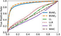
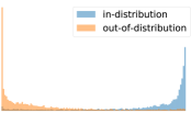
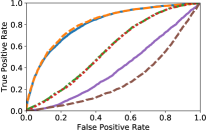
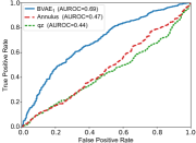
Figure 2: (Top row) ROC curves (left) and histograms of LL (middle) and BVAE₂ (right) scores on the FashionMNIST vs. MNIST task; BVAE₂ separates in-distribution and OoD data much more clearly than LL. (Bottom row) ROC curves for the SVHN vs. CIFAR10 (left) and latent space (right) task.

5.2 Out-of-Distribution Detection in Latent Space

While input space OoD detection is well-studied, latent space OoD detection has only recently been identified as a critical open problem [26, 22, 45, 4] (see also Section 1). Thus, there is a lack of suitable experimental benchmarks, making a quantitative evaluation challenging. A major issue in designing benchmarks based on commonly-used datasets such as MNIST is that it is unclear how to obtain ground truth labels for which latent points are OoD and which are not, as we require OoD labels for all possible latent points ${\mathbf{z}}^{*}\in{\mathbb{Z}}$, not just for those corresponding to inputs ${\mathbf{x}}^{*}$ from the given dataset. As a first step towards facilitating a systematic empirical evaluation of latent space OoD detection techniques, we propose the following experimental protocol. We use the BVAE₁ variant (see Section 5.1), as latent space detection does not require encoder robustness. We train the model on FashionMNIST (or potentially any other dataset), and then sample $N=10,000$ latent test points ${\mathbf{z}}^{*}$ from the Gaussian $\mathcal{N}(\mathbf{0},b\cdot{\mathbb{I}}_{d})$ where $b\in{\mathbb{R}}^{+}$ (we use $b=10,000$), following [45]. Since there do not exist ground truth labels for which latent points ${\mathbf{z}}^{*}$ are OoD or not, we compute a classifier-based OoD proxy score (to be detailed below) for each of the $N$ latent test points and then simply define the $N/2$ latents with the lowest scores to be in-distribution, and all others to be OoD.

To this end, we train an ensemble [38] of $J$ convolutional NN classifiers with parameters $\mathbf{W}=\{{\mathbf{w}}_{j}\}_{j=1}^{J}$ on FashionMNIST. We then approximate the novelty score for discriminative models proposed by [31], i.e., $Q_{\mathbf{W}}[{\mathbf{x}}^{*}]={\mathbb{H}}\left(\frac{1}{J}\sum_{{\mathbf{w}}\in\mathbf{W}}p(y|{\mathbf{x}}^{*},{\mathbf{w}})\right)-\frac{1}{J}\sum_{{\mathbf{w}}\in\mathbf{W}}{\mathbb{H}}(p(y|{\mathbf{x}}^{*},{\mathbf{w}}))$, where the first term is the entropy of the mixture $\frac{1}{J}\sum_{{\mathbf{w}}\in\mathbf{W}}p(y|{\mathbf{x}}^{*},{\mathbf{w}})$ of categorical distributions $p(y|{\mathbf{x}}^{*},{\mathbf{w}})$ (which is again categorical with averaged probits), and the second term is the average entropy of the predictive class distribution of the classifier with parameters ${\mathbf{w}}$. Alternatively, one could also use the closely related OoD score $\sum_{{\mathbf{w}}\in\mathbf{W}}\text{KL}(p(y|{\mathbf{x}}^{*},{\mathbf{w}})\|p(y|{\mathbf{x}}^{*},{\mathbb{D}}))$ of [38]. Since $Q_{\mathbf{W}}[{\mathbf{x}}^{*}]$ requires a test input ${\mathbf{x}}^{*}$, and we only have the latent code ${\mathbf{z}}^{*}$ corresponding to ${\mathbf{x}}^{*}$ in our setting, we instead consider the expected novelty under the mixture decoding distribution $p({\mathbf{x}}|{\mathbf{z}}^{*},{\mathbb{D}})$, $\mathbb{E}_{p({\mathbf{x}}|{\mathbf{z}}^{*},{\mathbb{D}})}[Q_{\mathbf{W}}[{\mathbf{x}}]]\simeq\frac{1}{L}\sum_{l=1}^{L}Q_{\mathbf{W}}[{\mathbf{x}}_{l}]$ with ${\mathbf{x}}_{l}\sim p({\mathbf{x}}|{\mathbf{z}}^{*},{\mathbb{D}})$. In practice, we use an ensemble of $J=5$ classifiers and $L=32$ input samples for the expectation. We compare the BVAE₁ model with our expected disagreement score $D_{\Theta}[{\mathbf{z}}^{*}]$ (see Section 3.2, with $N=32$ samples) against two baselines (which are the only existing methods we are aware of): (a) The distance of ${\mathbf{z}}^{*}\in{\mathbb{R}}^{d}$ to the spherical annulus of radius $\sqrt{d-1}$, which is where most probability mass lies under our prior $\mathcal{N}(\mathbf{0},{\mathbb{I}}_{d})$ (Annulus) [4], and (b) the log-probability of ${\mathbf{z}}^{*}$ under the aggregated posterior of the training data in latent space $q({\mathbf{z}})=\frac{1}{N}\sum_{{\mathbf{x}}\in{\mathbb{D}}}q({\mathbf{z}}|{\mathbf{x}},\phi)$, i.e., a uniform mixture of $N$ Gaussians in our case (qz) [45]. Fig. 2 (bottom right) shows that our method significantly outperforms the two baselines on this task.

6 Related Work

Supervised/Discriminative OoD detection methods. Most existing OoD detection approaches are task-specific in that they are applicable within the context of a given prediction task. As described in Section 1, these approaches train a deep discriminative model in a supervised fashion using the given labels. To detect outliers w.r.t. the target task, such approaches typically rely on some sort of confidence score to decide on the reliability of the prediction, which is either produced by modifying the model and/or training procedure, or computed/extracted post-hoc from the model and/or predictions [6, 64, 28, 40, 29, 61, 18, 66, 1]. Alternatively, some methods use predictive uncertainty estimates for OoD detection [21, 38, 46, 55, 56] (cf. Section 3.1). The main drawback of such approaches is that discriminatively trained models by design discard all input features which are not informative about the specific prediction task at hand, such that information that is relevant for general OoD detection might be lost. Thus, whenever the task changes, the predictive (and thus OoD detection) model must be re-trained from scratch, even if the input data remains the same.

Unsupervised/Generative OoD detection methods. task-agnostic OoD detection methods solely use the inputs for the unsupervised training of a DGM to capture the data distribution, which makes them independent of any prediction task and thus more general. Only a few recent works fall into this category. [58] propose to correct the likelihood $\log p({\mathbf{x}}^{*}|\theta)$ for confounding general population level background statistics captured by a background model $p({\mathbf{x}}^{*}|\theta_{0})$, resulting in the score $\log p({\mathbf{x}}^{*}|\theta)-\log p({\mathbf{x}}^{*}|\theta_{0})$. The background model $p({\mathbf{x}}^{*}|\theta_{0})$ is in practice trained by perturbing the data ${\mathbb{D}}$ with noise to corrupt its semantic structure, i.e., by sampling input dimensions i.i.d. from a Bernoulli distribution with rate $\mu\in[0.1,0.2]$ and replacing their values by uniform noise, e.g. $x_{i}\sim{\mathcal{U}}\{0,\ldots,255\}$ for images. [14] propose to use an ensemble [38] of independently trained likelihood-based DGMs (i.e., with random parameter initializations and random data shuffling) to approximate the Watanabe-Akaike Information Criterion (WAIC) [69] $\mathbb{E}_{p(\theta|{\mathbb{D}})}[\log p({\mathbf{x}}^{*}|\theta)]-\text{Var}_{p(\theta|{\mathbb{D}})}[\log p({\mathbf{x}}^{*}|\theta)]$, which provides an asymptotically correct likelihood estimate between the training and test set expectations (however, assuming a fixed underlying data distribution). Finally, [50] propose to account for the typicality of ${\mathbf{x}}^{*}$ via the score $\left|\log p({\mathbf{x}}^{*}|\theta)-\frac{1}{N}\sum_{{\mathbf{x}}\in{\mathbb{D}}}\log p({\mathbf{x}}|\theta)\right|$, although they focus on batches of test inputs instead of single inputs.

Latent space OoD detection. Many important problems in science and engineering involve optimizing an expensive black-box function over a highly structured (i.e., discrete or non-Euclidian) input space, e.g. graphs, sequences, or sets. Such problems are often tackled using Bayesian optimization (BO), which is an established framework for sample-efficient black-box optimization that has, however, mostly focused on continuous input spaces [11, 62]. To extend BO to structured input spaces, recent works either designed dedicated models and acquisition procedures to optimize structured functions in input space directly [7, 33, 17, 54], or instead train a deep generative model (e.g. a VAE) to map the structured input space onto a continuous latent space, where the optimization can then be performed using standard continuous BO techniques [22]. Despite recent successes of the latter so-called latent space optimization approach in areas such as automatic chemical design and automatic machine learning [22, 37, 51, 42, 41, 32, 67], it often progresses into regions of the latent space too far away from the training data, yielding meaningless or even invalid inputs. A few recent works have tried to detect/avoid the progression into out-of-distribution regions in latent space, by either designing the generative model to produce valid inputs [37, 16], or by explicitly constraining the optimization to stay in-distribution, which is quantified using certain proxy metrics [26, 45].

Bayesian DGMs. Only a few works have tried to do Bayesian inference in DGMs, none of which addresses OoD detection. While [36] describe how to do VI over the decoder parameters of a VAE (see their Appendix F), this is neither motivated nor empirically evaluated. [30] do mean-field Gaussian VI over the encoder and decoder parameters of an importance-weighted autoencoder [12] to increase model flexibility and improve generalization performance. [53] do mean-field Gaussian VI over the decoder parameters of a VAE to enable continual learning. [60] use SG-MCMC to sample the parameters of a generative adversarial network [25] to increase model expressiveness. [23] use SG-MCMC to sample the decoder parameters of a VAE for feature-wise active learning.

7 Conclusion

We proposed an effective method for unsupervised out-of-distribution detection, both in input space and in latent space, which uses information-theoretic metrics based on the posterior distribution over the parameters of a deep generative model (in particular a VAE). In the future, we want to explore extensions to other approximate inference techniques (e.g. variational inference [10]), and to other deep generative models (e.g., flow-based [35] or auto-regressive [68] models). Finally, we hope that this paper will inspire many follow-up works that will (a) develop further benchmarks and methods for the underappreciated yet critical problem of latent space OoD detection, and (b) further explore the described paradigm of information-theoretic OoD detection, which might be a promising approach towards the grand goal of making deep neural networks more reliable and robust.

Broader Impact

A sophisticated out-of-distribution detection mechanism will be a critical component of any machine learning pipeline deployed in a safety-critical application domain, such as healthcare or autonomous driving. Current algorithms are not able to identify scenarios in which they ought to fail, which is a major shortcoming, as that can lead to fatal decisions when deployed in decision-making pipelines. This severely limits the applicability of current state-of-the-art methods to such application domains, which substantially hinders the generally wide potential benefits that machine learning could have on society. We thus envision our approach to be beneficial and impactful in bringing deep neural networks and similar machine learning methods to such safety-critical applications. That being said, failure of our system could indeed lead to sub-optimal and potentially fatal decisions.

Appendix A Stochastic Gradient Markov Chain Monte Carlo (SG-MCMC)

To generate samples $\theta\sim p(\theta|{\mathbb{D}})$ of parameters $\theta$ of a DNN, one typically uses stochastic gradient MCMC methods such as stochastic gradient Hamiltonian Monte Carlo (SGHMC). In particular, consider the posterior distribution $p(\theta|{\mathbb{D}})\propto\exp(-U(\theta,{\mathbb{D}}))$ with potential energy function $U(\theta,{\mathbb{D}})=-\log p({\mathbb{D}},\theta)=-\log(p({\mathbb{D}}|\theta)p(\theta))=-\sum_{{\mathbf{x}}\in{\mathbb{D}}}\log p({\mathbf{x}}|\theta)-\log p(\theta)$ induced by the prior $p(\theta)$ and marginal log-likelihood $\log p({\mathbf{x}}|\theta)$. Hamiltonian Monte Carlo (HMC) [19, 8] is a method that generates samples $\theta\sim p(\theta|{\mathbb{D}})$ to efficiently explore the parameter space by simulating Hamiltonian dynamics, which involves evaluating the gradient $\nabla_{\theta}U(\theta)$ of $U$. However, computing this gradient requires examining the entire dataset ${\mathbb{D}}$ (due to the summation of the log-likelihood over all ${\mathbf{x}}\in{\mathbb{D}}$), which might be prohibitively costly for large datasets. To overcome this, [13] proposed SGHMC as a scalable HMC variant based on a noisy, unbiased gradient estimate $\nabla_{\theta}U(\theta,{\mathbb{M}})\simeq\nabla_{\theta}U(\theta,{\mathbb{D}})$ computed on a minibatch ${\mathbb{M}}$ of points sampled uniformly at random from ${\mathbb{D}}$ (i.e., akin to minibatch-based optimization algorithms such as stochastic gradient descent), i.e.,

$$\nabla_{\theta}U(\theta,{\mathbb{M}})=-\textstyle\frac{|{\mathbb{D}}|}{|{\mathbb{M}}|}\textstyle\sum_{{\mathbf{x}}\in{\mathbb{M}}}\nabla_{\theta}\log p({\mathbf{x}}|\theta)-\nabla_{\theta}\log p(\theta).$$ (5)

Appendix B Information-theoretic Perspective on the Proposed Disagreement Score

B.1 An Information-theoretic Perspective

Expanding on Section 3.2, we now provide a more principled justification for the disagreement score $D_{\Theta}[{\mathbf{x}}^{*}]$ in Eq. 4, which induces an information-theoretic perspective on OoD detection and reveals an intriguing connection to active learning. Assume that given training data ${\mathbb{D}}$ and a prior distribution $p(\theta)$ over the DGM parameters $\theta$, we have inferred a posterior distribution

$$p(\theta|{\mathbb{D}})=\frac{p({\mathbb{D}}|\theta)p(\theta)}{\int p({\mathbb{D}}|\theta)p(\theta)d\theta}=\frac{p({\mathbb{D}}|\theta)}{p({\mathbb{D}})}p(\theta)$$ (6)

over $\theta$. Then, for a given input ${\mathbf{x}}^{*}$, the score $D_{\Theta}[{\mathbf{x}}^{*}]$ quantifies how much the posterior $p(\theta|{\mathbb{D}})$ would change if we were to add ${\mathbf{x}}^{*}$ to ${\mathbb{D}}$ and then infer the augmented posterior

$$p(\theta|{\mathbb{D}}^{*})=\frac{p({\mathbf{x}}^{*}|\theta)p(\theta|{\mathbb{D}})}{\int p({\mathbf{x}}^{*}|\theta)p(\theta|{\mathbb{D}})d\theta}=\frac{p({\mathbf{x}}^{*}|\theta)}{p({\mathbf{x}}^{*}|{\mathbb{D}})}p(\theta|{\mathbb{D}})$$ (7)

based on this new training set ${\mathbb{D}}^{*}={\mathbb{D}}\cup\{{\mathbf{x}}^{*}\}$. To see this, first note that this change in the posterior is quantified by the normalized likelihood $\frac{p({\mathbf{x}}^{*}|\theta)}{p({\mathbf{x}}^{*}|{\mathbb{D}})}$, such that models $\theta$ under which ${\mathbf{x}}^{*}$ is more (less) likely – relative to all other models – will have a higher (lower) probability under the updated posterior $p(\theta|{\mathbb{D}}^{*})$. Now, given the samples $\{\theta_{m}\}_{m=1}^{M}$ of the old posterior $p(\theta|{\mathbb{D}})$, the normalized likelihood $\frac{p({\mathbf{x}}^{*}|\theta)}{p({\mathbf{x}}^{*}|{\mathbb{D}})}$ for a given model $\theta$ is proportional to $w_{\theta}$ in Eq. 4, i.e.,

$$\textstyle\frac{p({\mathbf{x}}^{*}|\theta)}{p({\mathbf{x}}^{*}|{\mathbb{D}})}\overset{(\ref{eq:expected_lik})}{=}\textstyle\frac{p({\mathbf{x}}^{*}|\theta)}{\mathbb{E}_{p(\theta|{\mathbb{D}})}[p({\mathbf{x}}^{*}|\theta)]}\simeq\textstyle\frac{p({\mathbf{x}}^{*}|\theta)}{\frac{1}{M}\sum_{\theta\in\Theta}p({\mathbf{x}}^{*}|\theta)}\overset{(\ref{eq:D_ess})}{=}Mw_{\theta}\ .$$ (8)

Thus, $w_{\theta}$ intuitively measures the relative usefulness of $\theta$ for describing the new posterior $p(\theta|{\mathbb{D}}^{*})$. More formally, the $[w_{\theta}]_{\theta\in\Theta}$ correspond to the importance weights of the samples $\theta\in\Theta$ drawn from the proposal distribution $p(\theta|{\mathbb{D}})$ for an importance sampling-based Monte Carlo approximation of an expectation w.r.t. the target distribution $p(\theta|{\mathbb{D}}^{*})$,

$$\mathbb{E}_{p(\theta|{\mathbb{D}}^{*})}[f(\theta)]\overset{(\ref{eq:smc})}{\simeq}\mathbb{E}_{p(\theta|{\mathbb{D}})}[Mw_{\theta}f(\theta)]\simeq\textstyle\sum_{\theta\in\Theta}w_{\theta}f(\theta)$$ (9)

for any function $f:\Theta\rightarrow{\mathbb{R}}$. The score $D_{\Theta}[{\mathbf{x}}^{*}]$ in Eq. 4 is a widely used measure of the efficiency of the estimator in Eq. 9, known as the effective sample size (ESS) of $\{\theta_{m}\}_{m=1}^{M}$ [47]. It quantifies how many i.i.d. samples drawn from the target posterior $p(\theta|{\mathbb{D}}^{*})$ are equivalent to the $M$ samples $\theta\in\Theta$ drawn from the proposal posterior $p(\theta|{\mathbb{D}})$ and weighted according to $w_{\theta}$, and thus indeed measures the change in distribution from $p(\theta|{\mathbb{D}})$ to $p(\theta|{\mathbb{D}}^{*})$. Equivalently, $D_{\Theta}[{\mathbf{x}}^{*}]$ can be viewed as quantifying the informativeness of ${\mathbf{x}}^{*}$ for updating the DGM parameters $\theta$ to the ones capturing the true density.

The OoD detection mechanism described in Section 3.2 can thus be intuitively summarised as follows: In-distribution inputs ${\mathbf{x}}^{*}$ are similar to the data points already in ${\mathbb{D}}$ and thus uninformative about the model parameters $\theta$, inducing small change in distribution from $p(\theta|{\mathbb{D}})$ to $p(\theta|{\mathbb{D}}^{*})$, resulting in a large ESS $D_{\Theta}[{\mathbf{x}}^{*}]$. Conversely, OoD inputs ${\mathbf{x}}^{*}$ are very different from the previous observations in ${\mathbb{D}}$ and thus informative about the model parameters $\theta$, inducing large change in the posterior, resulting in a small ESS $D_{\Theta}[{\mathbf{x}}^{*}]$.

Finally, this information-theoretic perspective on OoD detection reveals a close relationship to information-theoretic active learning [43, 31]. There, the same notion of informativeness (or, equivalently, disagreement) is used to quantify the novelty of an input ${\mathbf{x}}^{*}$ to be added to the data ${\mathbb{D}}$, aiming to maximally improve the estimate of the model parameters $\theta$ by maximally reducing the entropy / epistemic uncertainty in the posterior $p(\theta|{\mathbb{D}})$. This is further justified in the next section.

B.2 Further Justification

In Section B.1, we mentioned that the disagreement score $D_{\Theta}[{\mathbf{x}}^{*}]$ defined in Eq. 4 can be viewed as quantifying the informativeness of the input ${\mathbf{x}}^{*}$ for updating the DGM parameters $\theta$ to the ones capturing the true density, yielding an information-theoretic perspective on OoD detection and revealing a close relationship to information-theoretic active learning [43]. While this connection intuitively sensible, we now further describe and justify it.

In the paradigm of active learning, the goal is to iteratively select inputs ${\mathbf{x}}^{*}$ which improve our estimate of the model parameters $\theta$ as rapidly as possible, in order to obtain a decent estimate of $\theta$ using as little data as possible, which is critical in scenarios where obtaining training data is expensive (e.g. in domains where humans or costly simulations have to be queried to obtain data, which includes many medical or scientific applications). The main idea of information-theoretic active learning is to maintain a posterior distribution $p(\theta|{\mathbb{D}})$ over the model parameters $\theta$ given the training data ${\mathbb{D}}$ observed thus far, and to then select the new input ${\mathbf{x}}^{*}$ based on its informativeness about the distribution $p(\theta|{\mathbb{D}})$, which is measured by the change in distribution between the current $p(\theta|{\mathbb{D}})$ posterior and the updated posterior $p(\theta|{\mathbb{D}}^{*})$ with ${\mathbb{D}}^{*}={\mathbb{D}}\cup\{{\mathbf{x}}^{*}\}$. This change in the posterior distribution can, for example, be quantified by the cross-entropy or KL divergence between $p(\theta|{\mathbb{D}})$ and $p(\theta|{\mathbb{D}}^{*})$ [43], or by the decrease in entropy between $p(\theta|{\mathbb{D}})$ and $p(\theta|{\mathbb{D}}^{*})$ [31].

Intriguingly, while the problems of active learning and out-of-distribution detection have clearly distinct goals, they are fundamentally related in that they both critically rely on a reliable way to quantify how different an input ${\mathbf{x}}^{*}$ is from the training data ${\mathbb{D}}$ (or, put differently, how novel or informative ${\mathbf{x}}^{*}$ is). While in active learning, we aim to identify the input ${\mathbf{x}}^{*}$ that is maximally different (or novel / informative) in order to best improve our estimate of the model parameters by adding ${\mathbf{x}}^{*}$ to the training dataset ${\mathbb{D}}$, in out-of-distribution detection, we aim to classify a given input ${\mathbf{x}}^{*}$ as either in-distribution or OoD based on how different (or novel / informative) it is. This naturally suggests the possibility of leveraging methods to quantify the novelty / informativeness of an input ${\mathbf{x}}^{*}$ developed for one problem, and apply it to the other problem. However, most measures used in active learning are designed for continuous representations of the distributions $p(\theta|{\mathbb{D}})$ and $p(\theta|{\mathbb{D}}^{*})$, and are not directly applicable in our setting where $p(\theta|{\mathbb{D}})$ and $p(\theta|{\mathbb{D}})$ are represented by a discrete set of samples $\Theta$.

That being said, $D_{\Theta}[{\mathbf{x}}^{*}]$ can indeed be viewed as quantifying the change in distribution between the sample-based representations of $p(\theta|{\mathbb{D}})$ and $p(\theta|{\mathbb{D}}^{*})$ induced by ${\mathbf{x}}^{*}$ (and thus the informativeness of ${\mathbf{x}}^{*}$), revealing a link to information-theoretic active learning. In particular, [47] show that $D_{\Theta}[{\mathbf{x}}^{*}]$ (which corresponds to the effective sample size, as described in Section B.1) is closely related to the Euclidean distance between the vector of importance weights $\mathbf{w}=[w_{\theta}]_{\theta\in\Theta}$ and the vector $\mathbf{w}^{*}=[\frac{1}{M}]_{\theta\in\Theta}$ of probabilities defining the discrete uniform probability mass function, i.e.,

$$\|\mathbf{w}-\mathbf{w}^{*}\|_{2}=\sqrt{\frac{1}{D_{\Theta}[{\mathbf{x}}^{*}]}-\frac{1}{M}}\quad\Longleftrightarrow\quad D_{\Theta}[{\mathbf{x}}^{*}]=\frac{1}{\|\mathbf{w}-\mathbf{w}^{*}\|_{2}^{2}+\frac{1}{M}}$$ (10)

such that maximizing the score $D_{\Theta}[{\mathbf{x}}^{*}]$ is equivalent to minimizing the Euclidian distance $\|\mathbf{w}-\mathbf{w}^{*}\|_{2}$. Now, since

$$p(\theta|{\mathbb{D}}^{*})=\frac{p({\mathbf{x}}^{*}|\theta)p(\theta|{\mathbb{D}})}{\int p({\mathbf{x}}^{*}|\theta)p(\theta|{\mathbb{D}})d\theta}=\frac{p({\mathbf{x}}^{*}|\theta)}{p({\mathbf{x}}^{*}|{\mathbb{D}})}p(\theta|{\mathbb{D}})\overset{(\ref{eq:smc})}{\simeq}Mw_{\theta}p(\theta|{\mathbb{D}})\ ,$$ (11)

we observe that for a given model $\theta\in\Theta$, the posterior $p(\theta|{\mathbb{D}}^{*})$ is equal to $p(\theta|{\mathbb{D}})$ if and only if $Mw_{\theta}=1\Longleftrightarrow w_{\theta}=\frac{1}{M}$, such that $p(\theta|{\mathbb{D}}^{*})$ is equal to $p(\theta|{\mathbb{D}})$ for all models $\theta\in\Theta$ if and only if the weight vector $\mathbf{w}=[w_{\theta}]_{\theta\in\Theta}$ is equal to the vector $\mathbf{w}^{*}=[\frac{1}{M}]_{\theta\in\Theta}$ defining the discrete uniform probability mass function (pmf), in which case their Euclidian distance is minimized at $\|\mathbf{w}-\mathbf{w}^{*}\|_{2}=0$. As a result, the new posterior $p(\theta|{\mathbb{D}}^{*})$ is identical to the previous posterior $p(\theta|{\mathbb{D}})$ over the models $\theta\in\Theta$ (i.e., the change in the posterior is minimized) if and only if the score $D_{\Theta}[{\mathbf{x}}^{*}]$ is maximized to be $D_{\Theta}[{\mathbf{x}}^{*}]=M$. Conversely, the Euclidean distance is maximized at $\|\mathbf{w}-\mathbf{w}^{*}\|_{2}=\sqrt{(1-\frac{1}{M})}$ if and only if the weight vector is $\mathbf{w}=[0,\ldots,0,1,0,\ldots,0]$, in which case the new posterior is $p(\theta|{\mathbb{D}}^{*})=0$ for all $M-1$ models $\theta$ for which $w_{\theta}=0$, and $p(\theta|{\mathbb{D}}^{*})=Mp(\theta|{\mathbb{D}})$ for the single model $\theta$ for which $w_{\theta}=1$. Thus, the change between the new and previous posterior over the models $\theta\in\Theta$ is maximized if and only if the score $D_{\Theta}[{\mathbf{x}}^{*}]$ is minimized to be $D_{\Theta}[{\mathbf{x}}^{*}]=1$.

Finally, we observe that the notion of change in distribution for sample-based representations of posteriors captured by the Euclidian distance $\|\mathbf{w}-\mathbf{w}^{*}\|_{2}$ described above is closely related to the notion of change in distribution for continuous posterior representations. To see this, consider the Kullback-Leibler (KL) divergence, which is an information-theoretic measure for the discrepancy between distributions commonly used in information-theoretic active learning, defined as

$$\text{KL}[p(\theta|{\mathbb{D}})\|p(\theta|{\mathbb{D}}^{*})]=\int p(\theta|{\mathbb{D}})\log\frac{p(\theta|{\mathbb{D}})}{p(\theta|{\mathbb{D}}^{*})}d\theta\ .$$ (12)

We now show that maximizing our proposed OoD detection score $D_{\Theta}[{\mathbf{x}}^{*}]$ is equivalent to minimizing the KL divergence $\text{KL}[p(\theta|{\mathbb{D}})\|p(\theta|{\mathbb{D}}^{*})]$ between the previous posterior $p(\theta|{\mathbb{D}})$ and the new posterior $p(\theta|{\mathbb{D}}^{*})$, and vice versa, which is formalized in Proposition 1 below. This provides further evidence for the close connection between our proposed OoD detection approach and information-theoretic principles, and suggests that information-theoretic measures such as the KL divergence can be also used for OoD detection, yielding the paradigm of information-theoretic out-of-distribution detection.

Proposition 1.

Assume that the weights $w_{\theta}$ have some minimal, arbitrarily small, positive value $\varepsilon>0$, i.e., $w_{\theta}>\varepsilon,\forall\theta\in\Theta$. Also, assume that the KL divergence $\text{KL}[p(\theta|{\mathbb{D}})\|p(\theta|{\mathbb{D}}^{*})]$ is approximated based on a set $\Theta=\{\theta_{m}\}_{m=1}^{M}$ of samples $\theta_{m}\sim p(\theta|{\mathbb{D}})$. Then, an input ${\mathbf{x}}^{*}\in{\mathbb{X}}$ is a maximizer of $D_{\Theta}[{\mathbf{x}}^{*}]$ if and only if it is a minimizer of $\text{KL}[p(\theta|{\mathbb{D}})\|p(\theta|{\mathbb{D}}^{*})]$. Furthermore, an input ${\mathbf{x}}^{*}\in{\mathbb{X}}$ is a minimizer of $D_{\Theta}[{\mathbf{x}}^{*}]$ if and only if it is a maximizer of $\text{KL}[p(\theta|{\mathbb{D}})\|p(\theta|{\mathbb{D}}^{*})]$. Formally,

$$\operatorname{arg\,max}_{{\mathbf{x}}^{*}\in{\mathbb{X}}}D_{\Theta}[{\mathbf{x}}^{*}] =\operatorname{arg\,min}_{{\mathbf{x}}^{*}\in{\mathbb{X}}}\text{KL}[p(\theta|{\mathbb{D}})\|p(\theta|{\mathbb{D}}^{*})]\ ,$$ (13)

$$\operatorname{arg\,min}_{{\mathbf{x}}^{*}\in{\mathbb{X}}}D_{\Theta}[{\mathbf{x}}^{*}] =\operatorname{arg\,max}_{{\mathbf{x}}^{*}\in{\mathbb{X}}}\text{KL}[p(\theta|{\mathbb{D}})\|p(\theta|{\mathbb{D}}^{*})]\ .$$ (14)

Proof.

Reformulating the KL divergence in Eq. 12 and approximating it via our set $\Theta$ of posterior samples, we obtain

$$\text{KL}[p(\theta|{\mathbb{D}})\|p(\theta|{\mathbb{D}}^{*})] \overset{(\ref{eq:kl})}{=}\int p(\theta|{\mathbb{D}})\log\frac{p(\theta|{\mathbb{D}})}{p(\theta|{\mathbb{D}}^{*})}d\theta$$

$$=-\int p(\theta|{\mathbb{D}})\log\frac{p(\theta|{\mathbb{D}}^{*})}{p(\theta|{\mathbb{D}})}d\theta$$

$$\overset{(\ref{eq:new_post})}{=}-\int p(\theta|{\mathbb{D}})\log\frac{p({\mathbf{x}}^{*}|\theta)}{p({\mathbf{x}}^{*}|{\mathbb{D}})}d\theta$$

$$\overset{(\ref{eq:expected_lik})}{=}-\int p(\theta|{\mathbb{D}})\log\frac{p({\mathbf{x}}^{*}|\theta)}{\mathbb{E}_{p(\theta|{\mathbb{D}})}[p({\mathbf{x}}^{*}|\theta)]}d\theta$$

$$=-\mathbb{E}_{p(\theta|{\mathbb{D}})}\left[\log\frac{p({\mathbf{x}}^{*}|\theta)}{\mathbb{E}_{p(\theta|{\mathbb{D}})}[p({\mathbf{x}}^{*}|\theta)]}\right]$$

$$\simeq-\mathbb{E}_{p(\theta|{\mathbb{D}})}\left[\log\frac{p({\mathbf{x}}^{*}|\theta)}{\frac{1}{M}\sum_{\theta\in\Theta}p({\mathbf{x}}^{*}|\theta)}\right]$$

$$\simeq-\frac{1}{M}\sum_{\theta\in\Theta}\log\frac{p({\mathbf{x}}^{*}|\theta)}{\frac{1}{M}\sum_{\theta\in\Theta}p({\mathbf{x}}^{*}|\theta)}$$

$$\overset{(\ref{eq:D_ess})}{=}-\frac{1}{M}\sum_{\theta\in\Theta}\log Mw_{\theta}\ .$$ (15)

To see that Eq. 13 holds, observe that the sample-based approximation of $\text{KL}[p(\theta|{\mathbb{D}})\|p(\theta|{\mathbb{D}}^{*})]$ in Eq. 15 is indeed minimized to be $\text{KL}[p(\theta|{\mathbb{D}})\|p(\theta|{\mathbb{D}}^{*})]=0$ if and only if the weight vector $\mathbf{w}=[w_{\theta}]_{\theta\in\Theta}$ is equal to the vector $\mathbf{w}=[\frac{1}{M}]_{\theta\in\Theta}$ defining the discrete uniform pmf (and thus if and only if the score $D_{\Theta}[{\mathbf{x}}^{*}]$ is maximized to be $D_{\Theta}[{\mathbf{x}}^{*}]=M$), as then

$$\text{KL}[p(\theta|{\mathbb{D}})\|p(\theta|{\mathbb{D}}^{*})]\overset{(\ref{eq:kl_smp})}{\simeq}-\frac{1}{M}\sum_{\theta\in\Theta}\log Mw_{\theta}=-\frac{1}{M}M\log M\frac{1}{M}=-\log 1=0\ .$$ (16)

We now show Eq. 14. To see why we need the assumption that the weights $w_{\theta}$ have some minimal, arbitrarily small, positive value $\varepsilon>0$, i.e., $w_{\theta}\geq\varepsilon,\forall\theta\in\Theta$, consider the unconstrained case, where we know that $D_{\Theta}[{\mathbf{x}}^{*}]$ is minimized to be $D_{\Theta}[{\mathbf{x}}^{*}]=1$ if and only if the weight vector $\mathbf{w}=[w_{\theta}]_{\theta\in\Theta}$ is equal to the vector $\mathbf{w}=[0,\ldots,0,1,0,\ldots,0]$. While this weight vector indeed maximizes the sampling-based approximation of the KL divergence to be $\text{KL}[p(\theta|{\mathbb{D}})\|p(\theta|{\mathbb{D}}^{*})]=\infty$,

$$\text{KL}[p(\theta|{\mathbb{D}})\|p(\theta|{\mathbb{D}}^{*})]\overset{(\ref{eq:kl_smp})}{\simeq}-\frac{1}{M}\sum_{\theta\in\Theta}\log Mw_{\theta}=-\frac{1}{M}[\log M+(M-1)\log 0]=\infty\ ,$$ (17)

this maximizer is not unique, as any other weight vector containing at least one weight of $w_{\theta}=0$ equally achieves the maximum of $\text{KL}[p(\theta|{\mathbb{D}})\|p(\theta|{\mathbb{D}}^{*})]=\infty$. In theory, the KL divergence can thus not distinguish between weight vectors with different numbers of zero entries (i.e., different $\ell_{0}$-norms $\|\mathbf{w}\|_{0}$), although these clearly define different degrees of change in the discrete posterior representation. However, in practice, it is very unlikely to occur that any $w_{\theta}=0$. To obtain a unique maximizer of the KL divergence, we thus assume $w_{\theta}\geq\varepsilon,\forall\theta\in\Theta$ (where $\varepsilon>0$ can be chosen to be arbitrarily small), in which case $\text{KL}[p(\theta|{\mathbb{D}})\|p(\theta|{\mathbb{D}}^{*})]$ is maximized if and only if $\mathbf{w}=[\varepsilon,\ldots,\varepsilon,1-(M-1)\varepsilon,\varepsilon,\ldots,\varepsilon]$, in which case

$$\text{KL}[p(\theta|{\mathbb{D}})\|p(\theta|{\mathbb{D}}^{*})]\simeq-\frac{1}{M}\sum_{\theta\in\Theta}\log Mw_{\theta}=-\frac{1}{M}[\log M(1-(M-1)\varepsilon)+(M-1)\log M\varepsilon]<\infty\ .$$ (18)

The positivity assumption thus also ensures that the KL divergence remains bounded. To see why $\mathbf{w}=[\varepsilon,\ldots,\varepsilon,1-(M-1)\varepsilon,\varepsilon,\ldots,\varepsilon]$ maximizes the KL divergence, consider the alternative vector $\mathbf{w}=[\varepsilon,\ldots,\varepsilon,\varepsilon+\delta,\varepsilon,\ldots,\varepsilon,1-(M-1)\varepsilon-\delta,\varepsilon,\ldots,\varepsilon]$ where any of the entries with minimal value $\varepsilon$ is increased by some arbitrarily small, positive $\delta>0$, such that

$$\text{KL}[p(\theta|{\mathbb{D}})\|p(\theta|{\mathbb{D}}^{*})]\simeq-\frac{1}{M}\sum_{\theta\in\Theta}\log Mw_{\theta}-\frac{1}{M}[\log M(1-(M-1)\varepsilon-\delta)+(M-2)\log M\varepsilon+\log M(\varepsilon+\delta)]\ .$$ (19)

To see that adding such a $\delta$ decreases the value of the KL divergence, observe that Eq. 18 and Eq. 19 yield

$$\cancel{-\frac{1}{M}}[\log M(1-(M-1)\varepsilon)+(M-1)\log M\varepsilon] >\cancel{-\frac{1}{M}}[\log M(1-(M-1)\varepsilon-\delta)+(M-2)\log M\varepsilon+\log M(\varepsilon+\delta)]$$

$$\log M(1-(M-1)\varepsilon)+\cancel{(M-1)}\log M\varepsilon <\log M(1-(M-1)\varepsilon-\delta)+\cancel{(M-2)\log M\varepsilon}+\log M(\varepsilon+\delta)$$

$$\log\cancel{M}(1-(M-1)\varepsilon)+\log\cancel{M}\varepsilon <\log\cancel{M}(1-(M-1)\varepsilon-\delta)+\log\cancel{M}(\varepsilon+\delta)$$

$$\log(1-(M-1)\varepsilon)+\log\varepsilon <\log(1-(M-1)\varepsilon-\delta)+\log(\varepsilon+\delta)$$

$$\cancel{\log}(1-(M-1)\varepsilon)\varepsilon <\cancel{\log}(1-(M-1)\varepsilon-\delta)(\varepsilon+\delta)$$

$$(1-(M-1)\varepsilon)\varepsilon <(1-(M-1)\varepsilon-\delta)(\varepsilon+\delta)$$

$$\varepsilon-(M-1)\varepsilon^{2} <(\varepsilon+\delta)-(M-1)\varepsilon(\varepsilon+\delta)-\delta(\varepsilon+\delta)$$

$$\varepsilon-M\varepsilon^{2}+\varepsilon^{2} <\varepsilon+\delta-(M-1)(\varepsilon^{2}+\varepsilon\delta)-\varepsilon\delta-\delta^{2}$$

$$\varepsilon-M\varepsilon^{2}+\varepsilon^{2} <\varepsilon+\delta-[M\varepsilon^{2}+M\varepsilon\delta-\varepsilon^{2}-\varepsilon\delta]-\varepsilon\delta-\delta^{2}$$

$$\cancel{\varepsilon}\cancel{-M\varepsilon^{2}}+\cancel{\varepsilon^{2}} <\cancel{\varepsilon}+\delta\cancel{-M\varepsilon^{2}}-M\varepsilon\delta+\cancel{\varepsilon^{2}}+\cancel{\varepsilon\delta-\varepsilon\delta}-\delta^{2}$$

$$0 <\delta-M\varepsilon\delta-\delta^{2}$$

$$0 <1-M\varepsilon-\delta$$

$$M\varepsilon <1-\delta$$

$$\varepsilon <\frac{1-\delta}{M}\ .$$

The condition $\varepsilon<\frac{1-\delta}{M}$ implies that the largest weight in $\mathbf{w}$, denoted by $w_{\theta_{m}}$, satisfies

$$w_{\theta_{m}} =1-(M-1)\varepsilon-\delta$$

$$>1-(M-1)\frac{1-\delta}{M}-\delta$$

$$=1-\delta-\frac{M-M\delta-1+\delta}{M}$$

$$=\cancel{1-\delta-1+\delta}+\frac{1-\delta}{M}$$

$$=\frac{1-\delta}{M}$$

Thus, adding an arbitrarily small $\delta$ to one of the entries of $\mathbf{w}$ indeed decreases the value of the KL divergence, except when $\varepsilon=\frac{1-\delta}{M}$, in which case the KL divergences remains the same. However, in that case, the previously largest weight becomes $w_{\theta_{m}}=\frac{1-\delta}{M}=\varepsilon$, yielding the weight vector $\mathbf{w}=[\frac{1-\delta}{M},\ldots,\frac{1-\delta}{M},\frac{1-\delta}{M}+\delta,\frac{1-\delta}{M},\ldots,\frac{1-\delta}{M}]$, which is close to the discrete uniform pmf and thus results in a KL divergence close to zero (which is thus not relevant for characterizing the maximizer of the KL divergence). We can analogously identify $\mathbf{w}=[\varepsilon,\ldots,\varepsilon,1-(M-1)\varepsilon,\varepsilon,\ldots,\varepsilon]$ to be a minimizer of $D_{\Theta}[{\mathbf{x}}^{*}]$.

To conclude, since we can choose $\varepsilon$ to be arbitrarily small, it indeed holds that the KL divergence $\text{KL}[p(\theta|{\mathbb{D}})\|p(\theta|{\mathbb{D}}^{*})]$ is minimized if and only if the score $D_{\Theta}[{\mathbf{x}}^{*}]$ is maximized, which is when the importance weight vector defines the discrete uniform pmf, i.e., $\mathbf{w}=[\frac{1}{M}]_{\theta\in\Theta}$. Moreover, the KL divergence $\text{KL}[p(\theta|{\mathbb{D}})\|p(\theta|{\mathbb{D}}^{*})]$ is maximized if and only if the score $D_{\Theta}[{\mathbf{x}}^{*}]$ is minimized, which is when the importance weight vector is equal to $\mathbf{w}=[\varepsilon,\ldots,\varepsilon,1-(M-1)\varepsilon,\varepsilon,\ldots,\varepsilon]$. ∎

Appendix C Pseudocode of BVAE Training Procedure

Pseudocode for training a Bayesian VAE (for both variants 1 and 2, as described in Section 4) is shown in Algorithm 2, which is contrasted to the pseudocode for training a regular VAE in Algorithm 1 , allowing for a direct comparison between the closely related training procedures. In particular, in Algorithm 2, the parts in purple correspond to parts that are different from VAE training in Algorithm 1 and that apply to both BVAE variants 1 and 2. Furthermore, the parts in Algorithm 2 in blue correspond to BVAE variant 1 only, while the parts in red correspond to BVAE variant 2 only.

I.e., the training procedure of BVAE variant 1 is described by the union of all black, purple and blue parts in Algorithm 2, where the only difference to the regular VAE training procedure in Algorithm 1 is that an SG-MCMC sampler is used instead of an SGD optimizer for the decoder parameters $\theta$. The training procedure of BVAE variant 2 is described by the union of all black, purple and red parts in Algorithm 2, where, in contrast to the regular VAE training procedure in Algorithm 1, an SG-MCMC sampler is used instead of an SGD optimizer for both the decoder parameters $\theta$ and the encoder parameters $\phi$.

For the BVAE training procedure in Algorithm 2, we thus have to additionally specify the burn-in length $B$, which denotes the number of samples to discard at the beginning before storing any samples, as well as the sample distance $D$, which denotes the number of samples to discard in-between two subsequently stored samples (i.e., controlling the degree of correlation between the stored samples). This results in a total of $M=(T-B)/D+1$ samples for each sampling chain.

Regular VAE training in Algorithm 1 thus produces point estimates $\theta_{T}$ for the decoder parameters and $\phi_{T}$ for the encoder parameters, while Bayesian VAE training produces a set $\Theta=\{\theta_{B},\theta_{B+D},\theta_{B+2D},\ldots,\theta_{T}\}$ of posterior samples $\phi_{t}\sim p(\phi|{\mathbb{D}})$ of decoder parameters, as well as either a point estimate $\phi_{T}$ for the encoder parameters (in case of variant 1), or a set $\Phi=\{\phi_{B},\phi_{B+D},\phi_{B+2D},\ldots,\phi_{T}\}$ of posterior samples $\theta_{t}\sim p(\theta|{\mathbb{D}})$ of encoder parameters (in case of variant 2).

Note that just like the regular VAE training procedure in Algorithm 1, the Bayesian VAE training procedure in Algorithm 2 can in practice be conveniently implemented by exploiting automatic differentiation tools commonly employed by modern deep learning frameworks. Finally, as SG-MCMC methods are not much more expensive to run than stochastic optimization methods (i.e., both requiring a stochastic gradient step in every iteration, but SG-MCMC potentially requiring more iterations $T$ to generate $M$ diverse samples), training a Bayesian VAE is not significantly more expensive than training a regular VAE.

Algorithm 1 Regular VAE Training

  In. Dataset ${\mathbb{D}}$, mini-batch size $|{\mathbb{M}}|$, number of epochs $T$, generative model $p({\mathbf{x}},{\mathbf{z}},\theta)$, inference model $q({\mathbf{z}}|{\mathbf{x}},\phi)$

  $|$

  Initialize $\phi_{0}$ and $\theta_{0}$

  for $t=1,\ldots,T$ do

     Set $\hat{\phi}_{0}=\phi_{t-1}$, $\hat{\theta}_{0}=\theta_{t-1}$

     for $b=1,\ldots,\frac{|{\mathbb{D}}|}{|{\mathbb{M}}|}$ do

        Sample minibatch ${\mathbb{M}}\sim{\mathbb{D}}$

        Update $\hat{\phi}_{b-1}\rightarrow\hat{\phi}_{b}$ via SGD $\{$

        $|$

        Update $\hat{\theta}_{b-1}\rightarrow\hat{\theta}_{b}$ via SGD

     end for

     Set $\phi_{t}=\hat{\phi}_{\frac{|{\mathbb{D}}|}{|{\mathbb{M}}|}}$, $\theta_{t}=\hat{\theta}_{\frac{|{\mathbb{D}}|}{|{\mathbb{M}}|}}$

     $($

     $\{$

     

  end for

  Out. Decoder $\theta_{T}$ and encoder $\phi_{T}$ $\{$

  $|$

Algorithm 2 BVAE Training ( Variant 1 & 2)

  In. Dataset ${\mathbb{D}}$, mini-batch size $|{\mathbb{M}}|$, number of epochs $T$, generative model $p({\mathbf{x}},{\mathbf{z}},\theta)$, inference model $q({\mathbf{z}}|{\mathbf{x}},\phi)$, burn-in length $B$, sample distance $D$

  Initialize $\phi_{0}$ and $\theta_{0}$, and $\Theta=\emptyset$ and $\Phi=\emptyset$

  for $t=1,\ldots,T$ do

     Set $\hat{\phi}_{0}=\phi_{t-1}$, $\hat{\theta}_{0}=\theta_{t-1}$

     for $b=1,\ldots,\frac{|{\mathbb{D}}|}{|{\mathbb{M}}|}$ do

        Sample minibatch ${\mathbb{M}}\sim{\mathbb{D}}$

        Update $\hat{\phi}_{b-1}\rightarrow\hat{\phi}_{b}$ via $\{$ SGD $|$ SG-MCMC $\}$

        Update $\hat{\theta}_{b-1}\rightarrow\hat{\theta}_{b}$ via SG-MCMC

     end for

     Set $\phi_{t}=\hat{\phi}_{\frac{|{\mathbb{D}}|}{|{\mathbb{M}}|}}$, $\theta_{t}=\hat{\theta}_{\frac{|{\mathbb{D}}|}{|{\mathbb{M}}|}}$

     if $t\geq B$ and $(t-B)\text{ mod }D=0$ then

        Add $\Theta=\Theta\cup\{\theta_{t}\}$ and $\Phi=\Phi\cup\{\phi_{t}\}$

     end if

  end for

  Out. Decoder samples $\Theta$ and encoder $\{$ $\phi_{T}$ $|$ samples $\Phi$ $\}$

Appendix D Additional Plots for Experiments

We show additional plots for the experiments conducted in Section 5.

D.1 Score Histograms for SVHN vs. CIFAR10 Task

To complement the histograms of scores in Fig. 2 for the FashionMNIST vs. MNIST task, Fig. 3 shows similar behaviour for the corresponding histograms for the SVHN vs. CIFAR10 task.

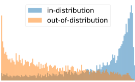
Figure 3: Histograms of LL (left) and BVAE₂ (right) scores on the SVHN vs. CIFAR10 task, again showing that BVAE₂ separates in-distribution and OoD data much more clearly than LL.

D.2 Further Precision-Recall and ROC Curves

We report precision-recall curves for all benchmarks, as well as ROC curves for the FashionMNIST (held-out classes) benchmark. We show both types of precision-recall curves, depending on whether in-distribution data are considered as the false class (denoted by "in"), or whether OoD data are considered to be the false class (denoted by "out"). Fig. 4 also shows examples from the FashionMNIST dataset, in order to help visualize the different class splits for the FashionMNIST (held-out class) benchmark.

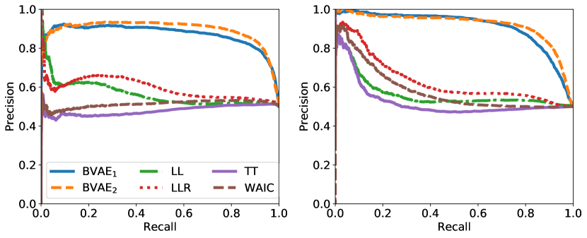
Figure 4: Precision-recall curves (in) and (out) on the FashionMNIST vs. MNIST benchmark.

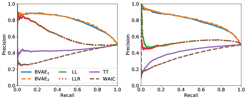
Figure 5: Precision-recall curves (in) and (out) on the SVHN vs. CIFAR10 benchmark.

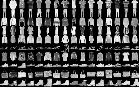
Figure 6: Examples from the FashionMNIST dataset for classes (from top to bottom) zero (t-shirt/top), one (trouser), two (pullover), three (dress), four (coat), five (sandal), six (shirt), seven (sneaker), eight (bag), and nine (ankle boot).

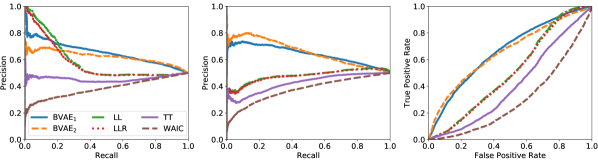
Figure 7: (Left) Precision-recall curves and (right) ROC curves of all methods on the FashionMNIST (held-out classes) benchmark with classes zero (t-shirt/top) and one (trouser) held-out.

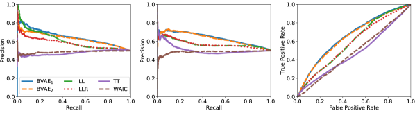
Figure 8: (From left to right) Precision-recall curves (in and out) and ROC curves of all methods on the FashionMNIST (held-out classes) benchmark with classes two (pullover) and three (dress) held-out.

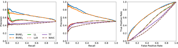
Figure 9: (From left to right) Precision-recall curves and ROC curves of all methods on the FashionMNIST (held-out classes) benchmark with classes four (coat) and five (sandal) held-out.

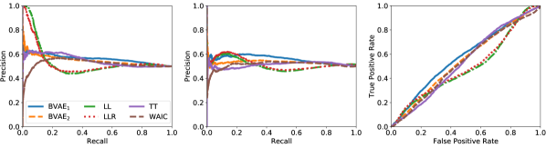
Figure 10: (From left to right) Precision-recall curves (in and out) and ROC curves of all methods on the FashionMNIST (held-out classes) benchmark with classes six (shirt) and seven (sneaker) held-out.

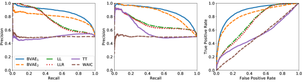
Figure 11: (From left to right) Precision-recall curves (in and out) and ROC curves of all methods on the FashionMNIST (held-out classes) benchmark with classes eight (bag) and nine (ankle boot) held-out.

References

- [1] F. Ahmed and A. Courville. Detecting semantic anomalies. arXiv preprint arXiv:1908.04388, 2019.
- [2] S. Akcay, A. Atapour-Abarghouei, and T. P. Breckon. Ganomaly: Semi-supervised anomaly detection via adversarial training. In Asian Conference on Computer Vision, pages 622–637. Springer, 2018.
- [3] A. A. Alemi, I. Fischer, and J. V. Dillon. Uncertainty in the variational information bottleneck. arXiv preprint arXiv:1807.00906, 2018.
- [4] Z. Alperstein, A. Cherkasov, and J. T. Rolfe. All smiles variational autoencoder. arXiv preprint arXiv:1905.13343, 2019.
- [5] D. Amodei, C. Olah, J. Steinhardt, P. Christiano, J. Schulman, and D. Mané. Concrete problems in ai safety. arXiv preprint arXiv:1606.06565, 2016.
- [6] J. An and S. Cho. Variational autoencoder based anomaly detection using reconstruction probability. Special Lecture on IE, 2(1), 2015.
- [7] R. Baptista and M. Poloczek. Bayesian optimization of combinatorial structures. arXiv preprint arXiv:1806.08838, 2018.
- [8] M. Betancourt. A conceptual introduction to hamiltonian monte carlo. arXiv preprint arXiv:1701.02434, 2017.
- [9] C. M. Bishop. Novelty detection and neural network validation. IEE Proceedings-Vision, Image and Signal processing, 141(4):217–222, 1994.
- [10] D. M. Blei, A. Kucukelbir, and J. D. McAuliffe. Variational inference: A review for statisticians. Journal of the American statistical Association, 112(518):859–877, 2017.
- [11] E. Brochu, V. M. Cora, and N. De Freitas. A tutorial on bayesian optimization of expensive cost functions, with application to active user modeling and hierarchical reinforcement learning. arXiv preprint arXiv:1012.2599, 2010.
- [12] Y. Burda, R. Grosse, and R. Salakhutdinov. Importance weighted autoencoders. arXiv preprint arXiv:1509.00519, 2015.
- [13] T. Chen, E. Fox, and C. Guestrin. Stochastic gradient hamiltonian monte carlo. In International conference on machine learning, pages 1683–1691, 2014.
- [14] H. Choi and E. Jang. Generative ensembles for robust anomaly detection. arXiv preprint arXiv:1810.01392, 2018.
- [15] C. Cremer, X. Li, and D. Duvenaud. Inference suboptimality in variational autoencoders. arXiv preprint arXiv:1801.03558, 2018.
- [16] H. Dai, Y. Tian, B. Dai, S. Skiena, and L. Song. Syntax-directed variational autoencoder for structured data. arXiv preprint arXiv:1802.08786, 2018.
- [17] E. Daxberger, A. Makarova, M. Turchetta, and A. Krause. Mixed-variable bayesian optimization. In Proceedings of the Twenty-Ninth International Joint Conference on Artificial Intelligence, IJCAI-20, pages 2633–2639, 2020.
- [18] T. DeVries and G. W. Taylor. Learning confidence for out-of-distribution detection in neural networks. arXiv preprint arXiv:1802.04865, 2018.
- [19] S. Duane, A. D. Kennedy, B. J. Pendleton, and D. Roweth. Hybrid monte carlo. Physics letters B, 195(2):216–222, 1987.
- [20] Y. Gal. Uncertainty in deep learning. University of Cambridge, 1:3, 2016.
- [21] Y. Gal and Z. Ghahramani. Dropout as a bayesian approximation: Representing model uncertainty in deep learning. In international conference on machine learning, pages 1050–1059, 2016.
- [22] R. Gómez-Bombarelli, J. N. Wei, D. Duvenaud, J. M. Hernández-Lobato, B. Sánchez-Lengeling, D. Sheberla, J. Aguilera-Iparraguirre, T. D. Hirzel, R. P. Adams, and A. Aspuru-Guzik. Automatic chemical design using a data-driven continuous representation of molecules. ACS central science, 4(2):268–276, 2018.
- [23] W. Gong, S. Tschiatschek, R. Turner, S. Nowozin, and J. M. Hernández-Lobato. Icebreaker: Element-wise active information acquisition with bayesian deep latent gaussian model. arXiv preprint arXiv:1908.04537, 2019.
- [24] I. Goodfellow, Y. Bengio, A. Courville, and Y. Bengio. Deep learning, volume 1. MIT Press, 2016.
- [25] I. Goodfellow, J. Pouget-Abadie, M. Mirza, B. Xu, D. Warde-Farley, S. Ozair, A. Courville, and Y. Bengio. Generative adversarial nets. In Advances in neural information processing systems, pages 2672–2680, 2014.
- [26] R.-R. Griffiths and J. M. Hernández-Lobato. Constrained bayesian optimization for automatic chemical design. arXiv preprint arXiv:1709.05501, 2017.
- [27] C. Guo, G. Pleiss, Y. Sun, and K. Q. Weinberger. On calibration of modern neural networks. In Proceedings of the 34th International Conference on Machine Learning-Volume 70, pages 1321–1330. JMLR. org, 2017.
- [28] D. Hendrycks and K. Gimpel. A baseline for detecting misclassified and out-of-distribution examples in neural networks. arXiv preprint arXiv:1610.02136, 2016.
- [29] D. Hendrycks, M. Mazeika, and T. G. Dietterich. Deep anomaly detection with outlier exposure. arXiv preprint arXiv:1812.04606, 2018.
- [30] D. Hernández-Lobato, T. D. Bui, Y. Li, J. M. Hernández-Lobato, and R. E. Turner. Importance weighted autoencoders with random neural network parameters. Workshop on Bayesian Deep Learning, NIPS 2016, 2016.
- [31] N. Houlsby, F. Huszár, Z. Ghahramani, and M. Lengyel. Bayesian active learning for classification and preference learning. arXiv preprint arXiv:1112.5745, 2011.
- [32] W. Jin, R. Barzilay, and T. Jaakkola. Junction tree variational autoencoder for molecular graph generation. arXiv preprint arXiv:1802.04364, 2018.
- [33] J. Kim, M. McCourt, T. You, S. Kim, and S. Choi. Bayesian optimization over sets. arXiv preprint arXiv:1905.09780, 2019.
- [34] D. P. Kingma and J. Ba. Adam: A method for stochastic optimization. arXiv preprint arXiv:1412.6980, 2014.
- [35] D. P. Kingma and P. Dhariwal. Glow: Generative flow with invertible 1x1 convolutions. In Advances in Neural Information Processing Systems, pages 10215–10224, 2018.
- [36] D. P. Kingma and M. Welling. Auto-encoding variational bayes. arXiv preprint arXiv:1312.6114, 2013.
- [37] M. J. Kusner, B. Paige, and J. M. Hernández-Lobato. Grammar variational autoencoder. In Proceedings of the 34th International Conference on Machine Learning-Volume 70, pages 1945–1954. JMLR. org, 2017.
- [38] B. Lakshminarayanan, A. Pritzel, and C. Blundell. Simple and scalable predictive uncertainty estimation using deep ensembles. In Advances in Neural Information Processing Systems, pages 6402–6413, 2017.
- [39] Y. LeCun, Y. Bengio, and G. Hinton. Deep learning. nature, 521(7553):436, 2015.
- [40] S. Liang, Y. Li, and R. Srikant. Enhancing the reliability of out-of-distribution image detection in neural networks. arXiv preprint arXiv:1706.02690, 2017.
- [41] X. Lu, J. Gonzalez, Z. Dai, and N. Lawrence. Structured variationally auto-encoded optimization. In International Conference on Machine Learning, pages 3273–3281, 2018.
- [42] R. Luo, F. Tian, T. Qin, E. Chen, and T.-Y. Liu. Neural architecture optimization. In Advances in Neural Information Processing Systems, pages 7827–7838, 2018.
- [43] D. J. MacKay. Information-based objective functions for active data selection. Neural computation, 4(4):590–604, 1992.
- [44] W. J. Maddox, P. Izmailov, T. Garipov, D. P. Vetrov, and A. G. Wilson. A simple baseline for bayesian uncertainty in deep learning. In Advances in Neural Information Processing Systems, pages 13132–13143, 2019.
- [45] O. Mahmood and J. M. Hernández-Lobato. A cold approach to generating optimal samples. arXiv preprint arXiv:1905.09885, 2019.
- [46] A. Malinin and M. Gales. Predictive uncertainty estimation via prior networks. In Advances in Neural Information Processing Systems, pages 7047–7058, 2018.
- [47] L. Martino, V. Elvira, and F. Louzada. Effective sample size for importance sampling based on discrepancy measures. Signal Processing, 131:386–401, 2017.
- [48] P.-A. Mattei and J. Frellsen. Refit your encoder when new data comes by. In 3rd NeurIPS workshop on Bayesian Deep Learning, 2018.
- [49] E. Nalisnick, A. Matsukawa, Y. W. Teh, D. Gorur, and B. Lakshminarayanan. Do deep generative models know what they don’t know? arXiv preprint arXiv:1810.09136, 2018.
- [50] E. Nalisnick, A. Matsukawa, Y. W. Teh, and B. Lakshminarayanan. Detecting out-of-distribution inputs to deep generative models using a test for typicality. arXiv preprint arXiv:1906.02994, 2019.
- [51] A. Nguyen, A. Dosovitskiy, J. Yosinski, T. Brox, and J. Clune. Synthesizing the preferred inputs for neurons in neural networks via deep generator networks. In Advances in neural information processing systems, pages 3387–3395, 2016.
- [52] A. Nguyen, J. Yosinski, and J. Clune. Deep neural networks are easily fooled: High confidence predictions for unrecognizable images. In Proceedings of the IEEE conference on computer vision and pattern recognition, pages 427–436, 2015.
- [53] C. V. Nguyen, Y. Li, T. D. Bui, and R. E. Turner. Variational continual learning. arXiv preprint arXiv:1710.10628, 2017.
- [54] C. Oh, J. M. Tomczak, E. Gavves, and M. Welling. Combinatorial bayesian optimization using graph representations. arXiv preprint arXiv:1902.00448, 2019.
- [55] K. Osawa, S. Swaroop, A. Jain, R. Eschenhagen, R. E. Turner, R. Yokota, and M. E. Khan. Practical deep learning with bayesian principles. arXiv preprint arXiv:1906.02506, 2019.
- [56] Y. Ovadia, E. Fertig, J. Ren, Z. Nado, D. Sculley, S. Nowozin, J. V. Dillon, B. Lakshminarayanan, and J. Snoek. Can you trust your model’s uncertainty? evaluating predictive uncertainty under dataset shift. arXiv preprint arXiv:1906.02530, 2019.
- [57] E. Parzen. On estimation of a probability density function and mode. The annals of mathematical statistics, 33(3):1065–1076, 1962.
- [58] J. Ren, P. J. Liu, E. Fertig, J. Snoek, R. Poplin, M. A. DePristo, J. V. Dillon, and B. Lakshminarayanan. Likelihood ratios for out-of-distribution detection. arXiv preprint arXiv:1906.02845, 2019.
- [59] D. J. Rezende, S. Mohamed, and D. Wierstra. Stochastic backpropagation and approximate inference in deep generative models. arXiv preprint arXiv:1401.4082, 2014.
- [60] Y. Saatci and A. G. Wilson. Bayesian GAN. In Advances in neural information processing systems, pages 3622–3631, 2017.
- [61] A. Shafaei, M. Schmidt, and J. J. Little. Does your model know the digit 6 is not a cat? a less biased evaluation of" outlier" detectors. arXiv preprint arXiv:1809.04729, 2018.
- [62] B. Shahriari, K. Swersky, Z. Wang, R. P. Adams, and N. De Freitas. Taking the human out of the loop: A review of bayesian optimization. Proceedings of the IEEE, 104(1):148–175, 2015.
- [63] R. Shu, H. H. Bui, S. Zhao, M. J. Kochenderfer, and S. Ermon. Amortized inference regularization. In Advances in Neural Information Processing Systems, pages 4393–4402, 2018.
- [64] M. Sölch, J. Bayer, M. Ludersdorfer, and P. van der Smagt. Variational inference for on-line anomaly detection in high-dimensional time series. arXiv preprint arXiv:1602.07109, 2016.
- [65] J. T. Springenberg, A. Klein, S. Falkner, and F. Hutter. Bayesian optimization with robust bayesian neural networks. In Advances in Neural Information Processing Systems, pages 4134–4142, 2016.
- [66] K. Sricharan and A. Srivastava. Building robust classifiers through generation of confident out of distribution examples. arXiv preprint arXiv:1812.00239, 2018.
- [67] A. Tripp, E. Daxberger, and J. M. Hernández-Lobato. Sample-efficient optimization in the latent space of deep generative models via weighted retraining. arXiv preprint arXiv:2006.09191, 2020.
- [68] A. Van den Oord, N. Kalchbrenner, L. Espeholt, O. Vinyals, A. Graves, et al. Conditional image generation with pixelcnn decoders. In Advances in neural information processing systems, pages 4790–4798, 2016.
- [69] S. Watanabe. Asymptotic equivalence of bayes cross validation and widely applicable information criterion in singular learning theory. Journal of Machine Learning Research, 11(Dec):3571–3594, 2010.
- [70] M. Yin and M. Zhou. Semi-implicit variational inference. arXiv preprint arXiv:1805.11183, 2018.
- [71] H. Zenati, C. S. Foo, B. Lecouat, G. Manek, and V. R. Chandrasekhar. Efficient gan-based anomaly detection. arXiv preprint arXiv:1802.06222, 2018.