Equivariant cohomology of a complexity-one four-manifold is determined by combinatorial data

Abstract.

For Hamiltonian circle actions on $4$-manifolds, we give a generators and relations description for the even part of the equivariant cohomology, as a module over the equivariant cohomology of a point. This description depends on combinatorial data encoded in the decorated graph of the manifold. We then give an explicit combinatorial description of all weak algebra isomorphisms. We use this description to prove that the even parts of the equivariant cohomology modules are weakly isomorphic (and the odd groups have the same ranks) if and only if the labelled graphs obtained from the decorated graphs by forgetting the height and area labels are isomorphic.

As a consequence, we give an example of an isomorphism of equivariant cohomology modules that cannot be induced by an equivariant diffeomorphism of spaces preserving a compatible almost complex structure. We also deduce a soft proof that there are finitely many maximal Hamiltonian circle actions on a fixed closed symplectic $4$-manifold.

1. Introduction

Beginning with work of Masuda [14], there have been a number of questions posed, and some answered, probing the extent to which equivariant cohomology is a complete invariant [6, 15]. For toric manifolds (in other words, smooth compact toric varieties), Masuda [14] related the equivariant cohomology module structure to the variety structure (the fan) defined by the toric manifold. More recently it was observed that to conclude that toric manifolds with isomorphic equivariant cohomology modules are isomorphic as varieties, an additional condition is required, namely that the equivariant cohomology module isomorphism must preserve the first equivariant Chern class [9, Remark 2.4(3)]. A special case of toric manifolds are toric symplectic manifolds: closed connected symplectic manifolds with a Hamiltonian action of a torus of half the dimension.

In this paper we look at the equivariant cohomology of a four-dimensional Hamiltonian $S^{1}$-space: a closed connected symplectic manifold equipped with a Hamiltonian $S^{1}$-action. Building on work of Audin [3] and Ahara and Hattori [1], Karshon [12] showed that a four-dimensional Hamiltonian $S^{1}$-space is determined by its decorated graph: a labelled graph indicating the isolated fixed points as thin vertices and the fixed surfaces as fat vertices; the vertices are vertically placed according to the moment map value and labelled by the height value, a fat vertex is also labelled by its symplectic area and genus; for a natural number $n>1$, an edge labelled $n$ between vertices indicates that the fixed points are connected by an invariant sphere whose stabilizer is the cyclic subgroup of $S^{1}$ of order $n$; see §2.2. We call the labelled graph obtained from the decorated graph by forgetting the height and area labels, and adding a vertex label indicating when an isolated vertex is extremal and a fat vertex label indicating its self intersection, the dull graph of the Hamiltonian $S^{1}$-space.

Equivariant cohomology in the sense of Borel is a generalized cohomology theory in the equivariant category. For a torus $T^{k}=(S^{1})^{k}$, the equivariant cohomology (over ${\mathbb{Z}}$) is defined to be

$$H_{T^{k}}^{*}(M;{\mathbb{Z}}):=H^{*}((M\times(S^{\infty})^{k})/T^{k};{\mathbb{Z}}),$$

where $S^{\infty}$ is the unit sphere in ${\mathbb{C}}^{\infty}$, the circle acts freely $S^{1}\mathbin{\raisebox{-0.5pt}{\reflectbox{\begin{sideways}$\circlearrowleft$\end{sideways}}}}S^{\infty}$ by coordinate multiplication, and $T^{k}\mathbin{\raisebox{-0.5pt}{\reflectbox{\begin{sideways}$\circlearrowleft$\end{sideways}}}}(M\times(S^{\infty})^{k})$ diagonally. In particular,

$$H^{*}_{T^{k}}(\operatorname{pt})=H^{*}((S^{\infty})^{k}/T^{k};{\mathbb{Z}})=H^{*}(({\mathbb{C}}{\mathbb{P}}^{\infty})^{k};{\mathbb{Z}})={\mathbb{Z}}[u_{1},\dots,u_{k}],\,\,\,\deg(u_{i})=2.$$

The constant map $\pi\colon M\to\operatorname{pt}$ induces a map $\pi^{*}\colon H^{*}_{T^{k}}(\operatorname{pt})\to H_{T^{k}}^{*}(M)$ which endows $H_{T^{k}}^{*}(M)$ with an $H^{*}_{T^{k}}(\operatorname{pt})$-module structure. We let $\cup$ denote the cup product in equivariant cohomology. We say that $H_{T^{k}}^{*}(M)$ and $H_{T^{k}}^{*}(N)$ are weakly isomorphic as modules if there is a ring isomorphism $f\colon H_{T^{k}}^{*}(M)\to H_{T^{k}}^{*}(N)$ and an automorphism $\gamma$ of $T^{k}$ such that $f(u\cup w)=\gamma^{*}(u)\cup f(w)$ for any $u\in H_{T^{k}}^{*}(\operatorname{pt})$ and $w\in H_{T^{k}}^{*}(M)$.

First, we obtain a generators and relations description of $H_{S^{1}}^{2*}(M)$ from the decorated graph. Moreover we express the module structure over $H_{S^{1}}^{*}(\operatorname{pt})={\mathbb{Z}}[t]$ in terms of these generators. See Theorem 4.3 for the explicit statement. In the proof of Theorem 4.3, we apply our previous results in [11, Theorem 1.1] that the inclusion of the fixed points set $i:M^{S^{1}}\hookrightarrow M$ induces an injection in integral equivariant cohomology

$$i^{*}:H^{*}_{S^{1}}(M;{\mathbb{Z}})\hookrightarrow H^{*}_{S^{1}}\left(M^{S^{1}};{\mathbb{Z}}\right)$$

and our characterization of the image of $i^{*}$ in equivariant cohomology with rational coefficients. We use the generators and relations description to relate the algebraic and combinatorial structures of the Hamiltonian $S^{1}$-action.

1.1 Theorem.

Let $S^{1}\mathbin{\raisebox{-0.5pt}{\reflectbox{\begin{sideways}$\circlearrowleft$\end{sideways}}}}(M,\omega_{M})$ and $S^{1}\mathbin{\raisebox{-0.5pt}{\reflectbox{\begin{sideways}$\circlearrowleft$\end{sideways}}}}(N,\omega_{N})$ be Hamiltonian $S^{1}$-spaces of dimension four. The following are equivalent.

1. The dull graphs of $M$ and $N$ are isomorphic as labelled graphs.

2. $H_{S^{1}}^{2*}(M)$ and $H_{S^{1}}^{2*}(N)$ are isomorphic as modules over $H_{S^{1}}^{*}(\operatorname{pt})$
   and $\operatorname{rank}H_{S^{1}}^{i}(M)=\operatorname{rank}H_{S^{1}}^{i}(N)$ for all odd $i$.

3. $H_{S^{1}}^{2*}(M)$ and $H_{S^{1}}^{2*}(N)$ are weakly isomorphic as modules over $H_{S^{1}}^{*}(\operatorname{pt})$
   and $\operatorname{rank}H_{S^{1}}^{i}(M)=\operatorname{rank}H_{S^{1}}^{i}(N)$ for all odd $i$.

Moreover we list all the weak isomorphisms of the even-dimensional equivariant cohomology as $H_{S^{1}}^{*}(pt)$-modules, and further check which weak isomorphisms send the first equivariant Chern class $c_{1}^{S^{1}}(TM)$ to $\pm c_{1}^{S^{1}}(TN)$. We consider the equivariant Chern classes of $TM$ as the equivariant Chern classes of the vector bundle $TM\to M$ equipped with an $S^{1}$-invariant complex structure $J\colon TM\to TM$ that is compatible with $\omega_{M}$; note that the equivariant Chern classes of $(TM,J)$ are independent of the choice of an invariant compatible complex structure on $TM$.

1.2 Corollary.

Let $S^{1}\mathbin{\raisebox{-0.5pt}{\reflectbox{\begin{sideways}$\circlearrowleft$\end{sideways}}}}(M,\omega_{M})$ and $S^{1}\mathbin{\raisebox{-0.5pt}{\reflectbox{\begin{sideways}$\circlearrowleft$\end{sideways}}}}(N,\omega_{N})$ be Hamiltonian $S^{1}$-spaces of dimension four. Let $f\colon H_{S^{1}}^{2*}(M)\to H_{S^{1}}^{2*}(N)$ be a weak isomorphism of modules. Assume that the rank of $H_{S^{1}}^{i}(M)$ equals the rank of $H_{S^{1}}^{i}(N)$ for $i=1,\,3$. Then

• $f(c_{1}^{S^{1}}(TM))=c_{1}^{S^{1}}(TN)$ if and only if $f$ is induced from a weak equivariant diffeomorphism $\widecheck{f}\colon M\to N$ such that for an $S^{1}$-invariant $\omega_{M}$-compatible complex structure $J_{M}$ on $M$, the structure

  $$\widecheck{f}_{*}{J_{M}}:=d\widecheck{f}\circ J_{M}\circ d\widecheck{f}^{-1}$$

  is $\omega_{N}$-compatible;

• $f(c_{1}^{S^{1}}(TM))=-c_{1}^{S^{1}}(TN)$ if and only if $f$ is induced from an equivariant diffeomorphism $\widecheck{f}\colon M\to N$ such that for an $S^{1}$-invariant $\omega_{M}$-compatible complex structure $J_{M}$ on $M$, the structure $-\widecheck{f}_{*}{J_{M}}$ is $\omega_{N}$-compatible.

We prove Theorem 1.1 and Corollary 1.2 in Section 7.

We note that there might be isomorphisms of equivariant cohomologies, as $H_{S^{1}}^{*}(pt)$-modules, that do not send $c_{1}^{S^{1}}(TM)$ to $c_{1}^{S^{1}}(TN)$ or to $-c_{1}^{S^{1}}(TN)$, explicitly the partial flips, defined in Section 7. We discovered the partial flip when trying to emulate Masuda’s work on toric manifolds. In that case, there are equivariant cohomology generators that are supported on $T$-invariant codimension $2$ submanifolds. These generators are in a certain sense unique. Trying to establish similar uniqueness properties of our generators has led us to some alternative generators, linear combinations of the original ones, that are not supported on $S^{1}$-invariant submanifolds. This led us to the partial flip isomorphism.

1.3 Example.

Consider the two Hamiltonian $S^{1}$-manifolds $S^{1}\mathbin{\raisebox{-0.5pt}{\reflectbox{\begin{sideways}$\circlearrowleft$\end{sideways}}}}(M,\omega_{M})$ and $S^{1}\mathbin{\raisebox{-0.5pt}{\reflectbox{\begin{sideways}$\circlearrowleft$\end{sideways}}}}(N,\omega_{N})$ with extended decorated graphs shown in Figure 1.4.

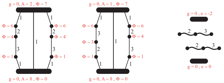
Figure 1.4. On the left are two extended graphs that differ by a partial flip. On the right is the dull graph that is the dull graph of each.

The $S^{1}$-manifolds $S^{1}\mathbin{\raisebox{-0.5pt}{\reflectbox{\begin{sideways}$\circlearrowleft$\end{sideways}}}}(M,\omega_{M})$ and $S^{1}\mathbin{\raisebox{-0.5pt}{\reflectbox{\begin{sideways}$\circlearrowleft$\end{sideways}}}}(N,\omega_{N})$ are obtained by precomposing the inclusion $S^{1}\hookrightarrow(S^{1})^{2}$ sending $s\mapsto(1,s)$ on the toric actions in Figure 1.5.

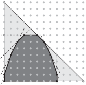
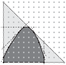
Figure 1.5. The moment map (Delzant) polytopes of the toric actions extending the $S^{1}$-actions.

Both toric actions are obtained from the toric action on $({\mathbb{C}}{\mathbb{P}}^{2},12\omega_{\text{FS}})$ by a sequence of $7$ equivariant blowups, of sizes $(5,4,3,2,2,1,1)$ in the left and $(5,4,4,2,2,1,1)$ in the right. The moment map polytopes define different fans, so the toric manifolds are different as toric varieties.

The decorated graphs in Figure 1.4 are not isomorphic, so Karshon’s work [12] implies that the two manifolds are not $S^{1}$-equivariantly symplectomorphic. The manifolds $M$ and $N$ are diffeomorphic: they are both $7$-fold blowups of ${\mathbb{C}}{\mathbb{P}}^{2}$, i.e., $6$-fold blowups of the non-trivial $S^{2}$-bundle over $S^{2}$. The blowup forms determining the symplectic structures are, in fact, distinct.

We show that the manifolds are not isomorphic by a weaker isomorphism: an equivariant diffeomorphism $\widecheck{f}\colon M\to N$ such that for an $S^{1}$-invariant $\omega_{M}$-compatible complex structure $J_{M}\colon TM\to TM$, either the complex structure $J_{N}:=\widecheck{f}_{*}J_{M}$ on $TN$ is $\omega_{N}$-compatible or the structure $J_{N}:=-\widecheck{f}_{*}J_{M}$ on $TN$ is $\omega_{N}$-compatible. Under such an isomorphism, we would have

(1.6) $${}\begin{array}[]{lcr}\widecheck{f}_{*}(c_{1}^{S^{1}}(TM))&=&\widecheck{f}_{*}(c_{1}^{S^{1}}(TM,J_{M}))\\ &=&c_{1}^{S^{1}}(TN,\widecheck{f}_{*}J_{M})\\ &=&\pm c_{1}^{S^{1}}(TN,J_{N})\\ &=&\pm c_{1}^{S^{1}}(TN).\end{array}$$

Moreover,

• The map $\widecheck{f}$ must send fixed points to fixed points.

• The map $\widecheck{f}$ sends an invariant $J_{M}$-holomorphic embedded sphere $S$ to an invariant $J_{N}$-holomorphic sphere. This is a consequence of the fact that in dimension $2$, every almost complex structure is integrable. So it is enough to show that $J_{N}T(\widecheck{f}(S))=T(\widecheck{f}(S))$, and indeed

  $$J_{N}T(\widecheck{f}(S))=d\widecheck{f}J_{M}d\widecheck{f}^{-1}d\widecheck{f}(TS)=d\widecheck{f}(J_{M}TS)=d\widecheck{f}(TS)=T(\widecheck{f}(S)).$$

• For each fixed point $p\in M$, $d\widecheck{f}_{p}\colon T_{p}M\to T_{\widecheck{f}(p)}N$ is an invariant $(J_{M},J_{N})$-complex linear isomorphism. Hence the weights of the $J_{N}$-complex representation at $\widecheck{f}(p)$ equal either the weights of the $J_{M}$-complex representation or their negation.

• The map $\widecheck{f}$ preserves or negates simultaneously the $J_{M}$-weights at fixed points that are the poles of an invariant $J_{M}$-holomorphic sphere $S$. This is a consequence of the fact that $T_{p}S$ ($T_{\widecheck{f}(p)}{\widecheck{f}(S)}$) is a complex linear subspace of $(T_{p}M,J_{M})$ ($(T_{p}N,J_{N})$), and for an $S^{1}$-action on a holomorphic $2$-sphere with fixed points $p$ and $q$, the weights at $p$ and $q$ have the same magnitude and opposite signs.

• Any edge in the decorated graph of $S^{1}\mathbin{\raisebox{-0.5pt}{\reflectbox{\begin{sideways}$\circlearrowleft$\end{sideways}}}}(M,\omega_{M})$ corresponds to an invariant $J_{M}$-holomorphic embedded sphere whose poles are fixed points [5, Lemma 2.4].

However, the compatibility with the symplectic form implies that the weights of the complex representation can be read from the graph, as in [12, §2]:

$$\big{\{}{\color[rgb]{0,0,1}\{-1,3\},\{-3,2\},\{-2,1\}},\{-1,3\},\{-3,2\},\{-2,1\}\big{\}}$$

at the isolated fixed points in $M$ and

$$\big{\{}{\color[rgb]{1,0,0}\{-1,2\},\{-2,3\},\{-3,1\},}\{-1,3\},\{-3,2\},\{-2,1\}\big{\}}$$

at the isolated fixed points in $N$. This and the facts above imply that $\widecheck{f}$ sends the isolated fixed points that are in a chain in $M$ to the isolated fixed points that are in a chain in $N$, but for one chain, the order (according to the moment map value) remains the same, and for the other chain, the order is reversed. We call the latter a flipped chain.

By [11, Corollary 4.9], relying on [7, Appendix C], at each isolated fixed point $\operatorname{pt}$, we have ${c_{1}^{S^{1}}}|_{\operatorname{pt}}=(-w_{1}-w_{2})t$, where $w_{1},\,w_{2}$ are the weights of the complex representation at $\operatorname{pt}$. Hence, for every fixed point $p$ in the flipped chain, we have

$${c_{1}^{S^{1}}(TN)}|_{F(p)}=-{c_{1}^{S^{1}}(TM)}|_{p}$$

and for every isolated fixed point $q$ in the other chain,

$${c_{1}^{S^{1}}(TN)}|_{F(q)}={c_{1}^{S^{1}}(TM)}|_{q}$$

contradicting (1.6).

Still, the two $S^{1}$-manifolds in Figure 1.4 have the same dull graph, thus, by Theorem 1.1, their equivariant cohomologies are isomorphic as modules. (Note that $g=0$ in both, hence $H_{S^{1}}^{2*+1}(M)=0=H_{S^{1}}^{2*+1}(N)$ and an isomorphism of the even part is an isomorphism of $H_{S^{1}}^{*}$.) Explicitly, the map $f:H_{S^{1}}^{2*}(M;{\mathbb{Z}})\to H_{S^{1}}^{2*}(N;{\mathbb{Z}})$ induced by the partial flip of the left chain is an isomorphism, see Proposition 7.12. $\diamondsuit$

As a further application of our generators and relations description, we deduce that there is a finite number of inequivalent maximal Hamiltonian circle actions on a fixed closed symplectic manifold $(M,\omega)$ of dimension four. A Hamiltonian torus action is maximal if it does not extend to a Hamiltonian action of a strictly larger torus on $(M,\omega)$. Karshon gives necessary and sufficient conditions for a Hamiltonian circle action on a $4$-manifold to extend to a toric one [12, Prop. 5.21]. In Figure 1.7, we show the extended graph and dull graph for a maximal Hamiltonian circle action. We call two torus actions equivalent if and only if they differ by an equivariant symplectomorphism composed with a reparametrization of the group ${(S^{1})}^{k}$.

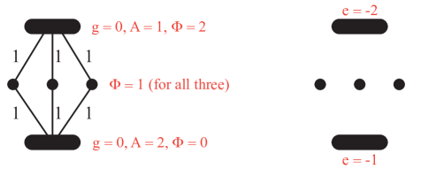
Figure 1.7. The extended graph and dull graph for a Hamiltonian circle action on a $4$-manifold that does not extend to a toric action. The manifold is diffeomorphic to a $4$-point blowup of ${\mathbb{C}}{\mathbb{P}}^{2}$.

1.8 Theorem.

Let $(M,\omega)$ be a connected closed $4$-dimensional symplectic manifold. The number of inequivalent maximal Hamiltonian torus actions on $(M,\omega)$ is finite.

We prove Theorem 1.8 in Section 8. The proof is analogous to the proof of McDuff and Borisov [16, Proposition 3.1] of the finiteness of toric actions on a given symplectic manifold. The key application of Hodge index theorem is similar. We use the fact that a Hamiltonian $S^{1}$-space of dimension four admits an invariant integrable complex structure that is compatible with the symplectic form, with respect to which the $S^{1}$-action is holomorphic. However some of the steps require an extra work. In particular, in Lemma 8.10 we give a formula for the classes $c_{1}(TM)$ and $c_{1}(TM)^{2}-2c_{2}({TM})$, using our generators. We note that this proof of the soft finiteness property is soft; it does not use hard pseudo-holomorphic tools. This is in contrast to the deduction of the finiteness from the characterization of the Hamiltonian circle actions on $(M,\omega)$ in [13] and [10], which both use pseudo-holomorphic curves.

Acknowledgements

We would like to thank Yael Karshon and Allen Knutson for helpful conversations. We also thank Susan Tolman and Mikiya Masuda for clarifying remarks. We are grateful to the anonymous referee for illuminating observations and corrections, and the patience of the editor as we implemented them. The first author was supported in part by the National Science Foundation under Grant DMS–1711317. Any opinions, findings, and conclusions or recommendations expressed in this material are those of the authors and do not necessarily reflect the views of the National Science Foundation. The second author was supported by the Israel Science Foundation, Grant 570/20.

2. Classification of Hamiltonian circle actions
on symplectic four-manifolds

We record here the details we will need resulting from the classification of Hamiltonian circle actions on symplectic four-manifolds [1, 3, 12]. An effective action of a torus $T={(S^{1})}^{k}$ on a symplectic manifold $(M,\omega)$ is Hamiltonian if there exists a moment map, that is, a smooth map $\Phi\colon M\to{\mathfrak{t}}^{*}\cong{{\mathbb{R}}}^{k}$ that satisfies Hamilton’s equation

$$d\Phi_{j}=-\iota(\xi_{j})\omega$$

for all $j=1,\dots,k$, where $\xi_{1},\ldots,\xi_{k}$ are the vector fields that generate the torus action.

In this paper we consider closed, connected Hamiltonian $S^{1}$-manifolds of dimension four. Hamilton’s equation guarantees that the set of fixed points of the $S^{1}$-action coincides with the critical set of a Morse-Bott function, the moment map $\Phi:M\to{\mathbb{R}}$. Moreover, the indices and dimensions of its critical submanifolds are all even, hence they can only consist of isolated points (with index $0$ or $2$ or $4$) and two-dimensional submanifolds (with index $0$ or $2$). The latter can only occur at the extrema of $\Phi$. By Morse-Bott theory (and since the manifold is connected), the maximum and minimum of the moment map is each attained on exactly one component of the fixed point set.

2.1.

Gradient spheres. An $S^{1}$-invariant Riemannian metric $\langle\cdot,\cdot\rangle$ on $(M,\omega,\Phi)$ is called compatible with $\omega$ if the automorphism $J\colon TM\to TM$ defined by $\langle\cdot,\cdot\rangle=\omega(\cdot,J\cdot)$ is an almost complex structure, i.e., $J^{2}=-\mathrm{Id}$. Such a $J$ is $S^{1}$-invariant. With respect to a compatible metric, the gradient vector field of the moment map, characterized by $\langle v,\operatorname{grad}\Phi\rangle=d\Phi(v)$, is

$$\operatorname{grad}\Phi=-J\xi_{M},$$

where $J$ is the corresponding almost complex structure and $\xi_{M}$ is the vector field that generates the $S^{1}$ action. The vector fields $\xi_{M}$ and $J\xi_{M}$ generate a ${\mathbb{C}}^{\times}=(S^{1})^{\mathbb{C}}$ action. The closure of a non-trivial ${\mathbb{C}}^{\times}$ orbit is a sphere, called a gradient sphere. These are collections of gradient flow lines for $\Phi$. On a gradient sphere, $S^{1}$ acts by rotation with two fixed points at the north and south poles; all other points on the sphere have the same stabilizer. We say that a gradient sphere is free if its stabilizer is trivial; otherwise it is non-free. For a smooth gradient sphere $S$ we have $JTS=TS$. Hence, since in dimension $2$ any almost complex structure is integrable, i.e., arises from an underlying complex atlas on the manifold, $S$ is a $J$-holomorphic sphere.

In dimension four, the existence of non-free gradient spheres does not depend on the compatible metric; each of these spheres coincides with a ${\mathbb{Z}}_{n}$-sphere for some $n>1$, which is a connected component of the closure of the set of points in $M$ whose stabilizer is equal to the cyclic subgroup of $S^{1}$ of order $n$ [12, Lemma 3.5].

All but a finite number of gradient spheres are free gradient spheres whose north and south poles are maximum and minimum of the moment map; we call the latter spheres trivial. A generic metric is one for which there exists no free gradient sphere whose north and south poles are both interior fixed points. For a generic compatible metric, the arrangement of gradient spheres is determined by the decorated graph defined below [12, Lemma 3.9].

2.2.

The decorated graph: conventions. To each connected four-dimensional Hamiltonian $S^{1}$-space, we associate a decorated graph as in [12]. We translate the moment map by a constant, if necessary, to fix the minimum value of the moment map to be $0$. For each isolated fixed point, there is a vertex labelled by its moment map value. For each fixed surface $\Sigma$, there is a fat vertex labelled by its moment map value, its symplectic area $\frac{1}{2\pi}\int_{\Sigma}\omega$, and its genus $g$. If there are two fat vertices, they necessarily have the same genus. If there is one fat vertex, it must have genus $0$ and the manifold $M$ is simply connected. If there are no fat vertices, the manifold is again simply connected and we say the genus is $0$. In this way, the genus is an invariant associated to the space $M$.

The moment map value determines the vertical placement of a (fat or isolated) vertex. The horizontal placement is for convenience and does not carry any significance. For each ${\mathbb{Z}}_{n}$-sphere, $n>1$, there is an edge connecting the vertices corresponding to its fixed points and labelled by the integer $n$. The edge-length is the difference of the moment map values of its vertices.

We recall the following facts.

• The sphere $S$ corresponding to an edge of label $n$ is a symplectic sphere whose size, $\frac{1}{2\pi}\int_{S}\omega$, is $\frac{1}{n}$ times the edge-length.

• For $n>1$, a fixed point has an isotropy weight $-n$ exactly when it is the north pole of a ${\mathbb{Z}}_{n}$-sphere, corresponding to a downward edge labelled $n$, and a weight $n$ exactly when it’s the south pole of a ${\mathbb{Z}}_{n}$-sphere.

• In particular, two edges incident to the same vertex have relatively prime edge labels, since the action is effective.

• A fixed point has an isotropy weight $0$ if and only if it lies on a fixed surface.

We denote

$$\operatorname{\sharp fat}:=\#\text{ fixed surfaces};\,\,\operatorname{\sharp iso}:=\#\text{ isolated fixed points};\,\,k:=\#\text{ chains of edges}.$$

2.3.

The extended graph: conventions. We define the extended decorated graph with respect to a compatible metric to be the graph obtained from the decorated graph as follows. We add edges labelled $1$ for each non-trivial free gradient sphere. We also add a redundant edge labelled $1$ for a trivial gradient sphere when $\operatorname{\sharp fat}\geq 1$ and $k<2$. In the resulting graph, every interior vertex is attached to one edge from above and one edge from below, the moment map labels remain monotone along each chain of edges, and there are at least two chains of edges. The length of one of the new edges is the difference of the moment map values of its vertices. In what follows, when we say extended decorated graph, we mean with respect a generic compatible Kähler metric.

2.4 Proposition.

In an extended decorated graph, we have the following.

1. If an edge has label $1$ then it is either the first or the last in a chain from $\mathrm{min}$ to $\mathrm{max}$ (or both).

2. For every interior fixed point that is not connected to top or bottom, there is exactly one edge from above and one edge from below, both with label $>1$.

3. Only edges of label $1$ can emanate from a fat vertex.

Proof.

The first item is a consequence of having a generic compatible metric on $(M,\omega,\Phi)$. This implies there exists no free gradient sphere whose north and south poles are both interior fixed points [12, Corollary 3.8]. The second item then follows from the first item and the construction of the extended graph. The third item is a consequence of the action being effective. ∎

2.5.

Topological invariants. Let $B_{\mathrm{min}}$ and $B_{\mathrm{max}}$ be the extremal critical sets of the moment map $\Phi$. For $*=\mathrm{min},\mathrm{max}$, we define

$$a_{*}=\int_{B_{*}}\omega\mbox{ ; }y_{*}=\Phi(B_{*})\mbox{ ; and }e_{*}=\left\{\begin{array}[]{ll}B_{*}\cdot B_{*}&\mbox{when }\dim(B_{*})=2\\ -\frac{1}{mn}&\mbox{when }\dim(B_{*})=0\end{array}\right.,$$

where $m$ and $n$ are the isotropy weights at $B_{*}$ when it is an isolated fixed point. In this case, $|m|$ and $|n|$ are the two largest labels emanating from the vertex corresponding to the point in an extended decorated graph. If $B_{*}$ is of $\dim 2$ we denote it by $\Sigma_{*}$. For an interior isolated fixed point $p$, we define $y_{p}=\Phi(p),$ and let $m_{p}$ and $n_{p}$ be the absolute values of the isotropy weights at $p$; these are the labels of the edges emanating from the vertex corresponding to $p$ in an extended decorated graph. We let $e_{p}=\frac{1}{m_{p}n_{p}}$.

These parameters are related by the following formulæ.

(2.6) $${}e_{\mathrm{min}}=\frac{\left(\sum_{p}y_{p}e_{p}\right)+a_{\mathrm{min}}-\left(\sum_{p}e_{p}\right)\cdot y_{\mathrm{max}}-a_{\mathrm{max}}}{y_{\mathrm{max}}-y_{\mathrm{min}}}$$

and

(2.7) $${}e_{\mathrm{max}}=\frac{\left(\sum_{p}e_{p}\right)\cdot y_{\mathrm{min}}+a_{\mathrm{max}}-\left(\sum_{p}y_{p}e_{p}\right)-a_{\mathrm{min}}}{y_{\mathrm{max}}-y_{\mathrm{min}}},$$

where $p$ runs over the interior fixed points. Formulæ (2.6) and (2.7) can be deduced from [12, Proof of Lemma 2.18], which has a missing term that we have restored (the missing term is the $a_{\mathrm{max}}$; its absence does not affect the validity of Karshon’s proof).

The proofs in Sections 3, 4 and 5 require recalling the details of the characterization of Hamiltonian $S^{1}$-spaces of dimension four. We recall these here.

2.8.

Circle actions that extend to toric actions. Consider a toric symplectic four-manifold $T\mathbin{\raisebox{-0.5pt}{\reflectbox{\begin{sideways}$\circlearrowleft$\end{sideways}}}}(M,\omega)$. An inclusion

$$\operatorname{inc}\colon S^{1}\hookrightarrow T={(S^{1})}^{2};\,\,s\mapsto(s^{m},s^{n})$$

induces a projection on the duals of the Lie algebras ${{\mathbb{R}}}^{2}\to{\mathbb{R}}$ defined by $(m,n)\in{{\mathbb{Z}}}^{2}$, explicitly ${{\mathbb{R}}}^{2}\ni(x,y)\mapsto mx+ny$. Composing this projection on the moment map of the torus action yields the moment map of the circle action.

2.9 Notation.

For the $S^{1}$-action to be effective, the pair $(m,n)$ is either $\pm(1,0)$, $\pm(0,1)$, or satisfies $\gcd(m,n)=1$. In what follows, we will frequently need to use this fact. We fix $a,b\in{\mathbb{Z}}$ are such that

(2.10) $$am-bn=1.$$

When $(m,n)=\pm(1,0)$, we take $a=\pm 1$ and $b=0$; when $(m,n)=\pm(0,1)$, we take $a=0$ and $b=\mp 1$; and when $(m,n)=\pm(1,1)$, we take $a=0$ and $b=\mp 1$. These then still satisfy (2.10).

The fixed surfaces are the preimages, under the $T$-moment map, of the edges of the Delzant polytope parallel to $(-n,m)$. Such a surface has genus zero and its normalized symplectic area equals the affine length of the corresponding edge. The isolated fixed points are the preimages of the vertices of the polygon that do not lie on such edges. To determine the $S^{1}$ isotropy of a $T$-invariant sphere, if the image under the $T$-moment map is parallel to the primitive vector $e=(\alpha,\beta)$, then relative to the circle action, the sphere is a ${\mathbb{Z}}_{\ell}$ sphere for $\ell=|m\alpha+n\beta|$. For further details, see [12, §2.2]. An example is shown in Figure 2.11.

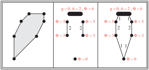
Figure 2.11. A moment polytope for a toric $4$-manifold on the left, together with the decorated graph and extended graph for the second coordinate circle action.

2.12 Example.

The complex projective plane ${\mathbb{C}}{\mathbb{P}}^{2}$ with a multiplication of the Fubini-Study form $\omega_{\text{FS}}$ by $\lambda>0$ admits the toric action

$$(t_{1},t_{2})\cdot[z_{0};z_{1};z_{2}]=[z_{0};t_{1}z_{1};t_{2}z_{2}]$$

whose moment map is the Delzant triangle of edge-length $\lambda$. Denote by $L$ the homology class of a line ${\mathbb{C}}{\mathbb{P}}^{1}$ in ${\mathbb{C}}{\mathbb{P}}^{2}$. For each of the edges of the Delzant triangle, its preimage is an invariant embedded holomorphic and symplectic sphere in $L$. For $(m,n)\in{{\mathbb{Z}}}^{2}$ with $\gcd(m,n)=1$ the inclusion $s\mapsto(s^{m},s^{n})$ induces the circle action

$$s\cdot[z_{0};z_{1};z_{2}]=[z_{0};s^{m}z_{1};s^{n}z_{2}].$$

For the $T$-moment map, the edges of the Delzant triangle lie on the lines $x=0$, $y=0$, and $x+y=1$, as shown in Figure 2.13(a). Thus there is an $S^{1}$-fixed sphere exactly when $(m,n)$ is $\pm(1,0)$, $\pm(0,1)$ and $\pm(1,1)$. Otherwise, there are a ${\mathbb{Z}}_{|m-n|}$-sphere, a ${{\mathbb{Z}}}_{|n|}$-sphere, and a ${{\mathbb{Z}}}_{|m|}$-sphere: $[0;z_{1};z_{2}],\,\,[z_{0};0;z_{2}],\,\,[z_{0},z_{1},0]$, respectively. See Figure 2.13 for the corresponding labeled graphs. In all cases, the Kähler metric is generic.

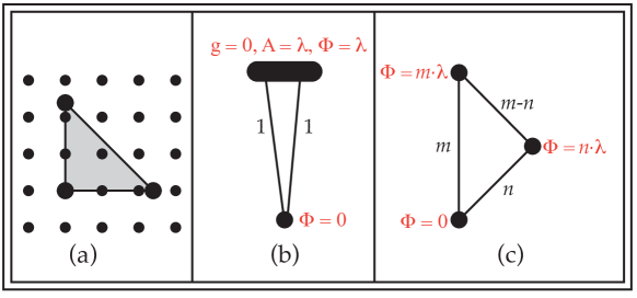
Figure 2.13. The $T^{2}$ moment map image and some possible extended graphs for a Hamiltonian circle action on ${\mathbb{C}}{\mathbb{P}}^{2}$. In (c), we are assuming $m>n>0$.

2.14 Example.

We denote by $\operatorname{Hirz}_{N}$ the Hirzebruch surface that is the algebraic submanifold of ${\mathbb{C}}{\mathbb{P}}^{1}\times{\mathbb{C}}{\mathbb{P}}^{2}$ defined in homogeneous coordinates by

$$\{([w_{1};w_{2}],[z_{0};z_{1};z_{2}])\in{\mathbb{C}}{\mathbb{P}}^{1}\times{\mathbb{C}}{\mathbb{P}}^{2}\mid w_{1}^{N}z_{2}=w_{2}^{N}z_{1}\}.$$

For $\beta,f>0$, we denote by $\eta_{\beta,f}$ the sum of the Fubini-Study form on ${\mathbb{C}}{\mathbb{P}}^{1}$ multiplied by $\beta$ and the Fubini-Study form on ${\mathbb{C}}{\mathbb{P}}^{2}$ multiplied by $f$. We shall use the same notation for its restriction to the Hirzebruch surface. The zero section $S_{0}$ is the sphere $\{([w_{1};w_{2}],[1;0;0])\}$, the section at infinity $S_{\infty}$ is the sphere $\{([w_{1};w_{2}],[0,w_{1}^{N},;w_{2}^{N}])\}$, and the fiber at zero $F_{0}$ is the sphere $\{([1;0],[z_{0};z_{1};0])\}$.

The Hirzebruch surface $(\operatorname{Hirz}_{N},\eta_{\beta,f})$ admits the toric action

$$(s,t)\cdot([w_{1};w_{2}],[z_{0};z_{1};z_{2}])=([w_{1};sw_{2}],[tz_{0};z_{1};s^{N}z_{2}])$$

whose moment map image is the trapezoid in Figure 2.15. The parameter $\beta$ is the average width of the trapezoid, $f$ is the height, and $\frac{1}{N}$ is the slope of the right edge if $N>0$, the right edge is vertical is $N=0$. We assume that $\beta\geq f$ and that $\beta-N\frac{f}{2}>0$. For $(m,n)\in{{\mathbb{Z}}}^{2}$ with $\gcd(m,n)=1$ the inclusion $s\mapsto(s^{m},s^{n})$ induces the circle action

$$\xi\cdot([w_{1};w_{2}],[z_{0};z_{1},;z_{2}])=([w_{1};\xi^{m}w_{2}],[\xi^{n}z_{0};z_{1};\xi^{Nm}z_{2}]).$$

There are two fixed spheres if $(m,n)=\pm(0,1)$. The circle action has exactly one fixed sphere and one ${{\mathbb{Z}}}_{N}$-sphere if $(m,n)=\pm(1,0)$. Otherwise, there are two ${{\mathbb{Z}}}_{|m|}$-spheres, a ${\mathbb{Z}}_{|mN-n|}$-sphere, and a ${{\mathbb{Z}}}_{|n|}$-sphere. The decorated graphs for these actions are shown in Figure 2.16.

In these examples, the Kähler metric is generic except for graph (d) with $m=1$, . However, these non-generic Hamiltonian $S^{1}$-spaces are each isomorphic to a space whose graph is of type (c) with $N^{\prime}=N-2|n|$ (and $m,|n|$ as before); the Kähler metric on that isomorphic space is generic. For further details, see [12, Remark 6.12].

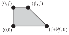
Figure 2.15. The standard Hirzebruch trapezoid

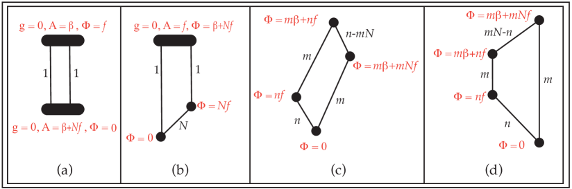
Figure 2.16. Some possible extended graphs for a Hamiltonian circle action on a Hirzebruch surface. In (c) and (d), we are assuming $m,n>0$. In (c), we have $n-mN>0$ and in (d), $mN-n>0$.

2.17 Notation.

Consider an $S^{2}$-bundle over a closed Riemann surface $\Sigma$. We fix basepoints $\ast\in S^{2}$ and $\ast\in\Sigma$. For the trivial $S^{2}$-bundle $\Sigma\times S^{2}$ over $\Sigma$, we denote $F:=[\ast\times S^{2}],\,\,\,B^{*}:=B=[\Sigma\times\ast],$ classes in the homology group $H_{2}(\Sigma\times S^{2};{\mathbb{Z}})$. When we consider the non-trivial $S^{2}$-bundle $M_{\Sigma}\stackrel{{\scriptstyle\pi}}{{\to}}\Sigma$, denote the homology class of the fiber by $F=[\pi^{-1}(\ast)]\in H_{2}(M_{\Sigma};{\mathbb{Z}})$. For each $\ell$, the trivial bundle admits a section ${\sigma}_{2\ell}:\Sigma\to\Sigma\times S^{2}$ whose image $\sigma_{2\ell}(\Sigma)$ has even self intersection number $2\ell$. Similarly, for each $\ell$, the non-trivial bundle admits a section $\sigma_{2\ell+1}:\Sigma\to M_{\Sigma}$ whose image $\sigma_{2\ell+1}(\Sigma)$ has odd self intersection number $2\ell+1$. We denote $B_{n}:=[\sigma_{n}(\Sigma)]\in H_{2}(M_{\Sigma};{\mathbb{Z}})$. For every $n\in{\mathbb{Z}}$, we have $B_{n}=B_{-n}+nF.$ When we consider the non-trivial $S^{2}$-bundle denote $B^{*}:=\frac{1}{2}(B_{1}+B_{-1})$ in $H_{2}(M_{\Sigma};{\mathbb{Q}})$. Note that

(2.18) $$B^{*}=\frac{1}{2}(B_{n}+B_{-n})$$

for all even $n$ in the trivial case, and for all odd $n$ in the non-trivial case. A Hirzebruch surface is an $S^{2}$-bundle over $S^{2}$. In $\operatorname{Hirz}_{N}$, we have $S_{0}=B_{N}$, $S_{\infty}=B_{-N}$ and $F_{0}=F$

An $S^{2}$-bundle over $\Sigma$ with a circle action that fixes the basis and rotates each fiber, an invariant symplectic form $\omega$ and a moment map is called a symplectic $S^{1}$-ruled surface. It admits a ruled complex analytic structure as an $S^{2}$-bundle over $(\Sigma,j)$, that is compatible with the $S^{1}$-action and with $\omega$, such that the Kähler metric is generic. Its decorated graph is as in Figure 2.16(a), with genus labels $g\geq 0$.

2.19.

The effect of a blowup on the decorated graph. Let $J$ be an integrable $\omega$-compatible complex structure on a Hamiltonian $S^{1}\mathbin{\raisebox{-0.5pt}{\reflectbox{\begin{sideways}$\circlearrowleft$\end{sideways}}}}(M^{4},\omega)$ with respect to which the $S^{1}$-action is holomorphic. Let $p$ be a fixed point in $M$. Let $U\subset M$ be an invariant open ball centered around the fixed point $p$, small enough such that the $S^{1}$-action on $U$ is linear (in holomorphic coordinates). In particular it induces an $S^{1}$-action on the manifold $\widetilde{U}=\{(z,l)\colon z\in l\}\subset U\times{\mathbb{C}}{\mathbb{P}}^{1}$. The equivariant complex blowup $\widetilde{M}$ of $M$ at $p$ is the complex $S^{1}$-manifold

(2.20) $${}\widetilde{M}=M\smallsetminus\{p\}\cup\widetilde{U},$$

obtained by adjoining $M\smallsetminus\{p\}$ with $\widetilde{U}$ via the equivariant isomorphism $\widetilde{U}\smallsetminus(z=0)\cong U\smallsetminus\{p\}$ given by $(z,l)\mapsto z$. There is a natural equivariant projection

(2.21) $${}{\mathbb{B}\hskip-1.084pt\mathbb{L}}\colon\widetilde{M}\to M$$

extending the identity on $M\smallsetminus\{p\}$. The inverse image ${{\mathbb{B}\hskip-1.084pt\mathbb{L}}}^{-1}(p)$ is naturally isomorphic to ${\mathbb{C}}{\mathbb{P}}^{1}$ and is called the exceptional divisor of the blowup; it is $S^{1}$-invariant. Let $E$ be the homology class in $H_{2}(\widetilde{M};{\mathbb{Z}})$ of the exceptional divisor. In $k$-fold complex blowup we denote the classes of the exceptional divisors by $E_{1},\ldots,E_{k}$.

For $\lambda>0$, define a $\lambda$-blowup of the decorated graph, according to the location of the blowup, as in Figure 2.22. We say that the obtained graph is valid if the (fat or not) vertices created in the $\lambda$-blowup do not surpass the other pre-existing (fat or not) vertices in the same chain of edges, and the fat vertices after the $\lambda$-blowup have positive size labels. If the $\lambda$-blowup of the decorated graph is valid, then there exists an invariant Kähler form $\widetilde{\omega}$ on the equivariant complex blowup in the cohomology class

$${\mathbb{B}\hskip-1.084pt\mathbb{L}}^{*}[\omega]-\lambda\Xi,$$

where $\Xi$ is the Poincaré dual of the exceptional divisor class $E$, and the graph of the blowup $S^{1}\mathbin{\raisebox{-0.5pt}{\reflectbox{\begin{sideways}$\circlearrowleft$\end{sideways}}}}(\widetilde{M},\widetilde{\omega})$ is this $\lambda$-blownup graph. By [12, Theorem 7.1], if the Kähler metric on $S^{1}\mathbin{\raisebox{-0.5pt}{\reflectbox{\begin{sideways}$\circlearrowleft$\end{sideways}}}}(M,\omega)$ is generic, then so is the resulting Kähler metric on $S^{1}\mathbin{\raisebox{-0.5pt}{\reflectbox{\begin{sideways}$\circlearrowleft$\end{sideways}}}}(\widetilde{M},\widetilde{\omega})$.

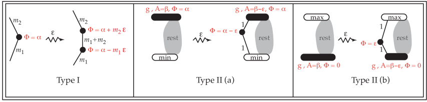
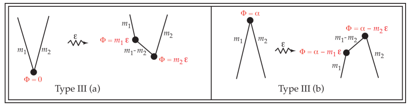
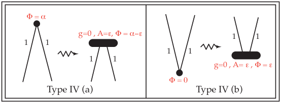
Figure 2.22. The effect on the decorated graph of Types I–IV blowups. Note that in Type III(a) and IV(b), the final moment map should be corrected with a vertical translation to comply with the convention that the minimum moment map value is $\Phi=0$.

2.23.

Equivariant blowdown. By the Castelnuovo-Enriques criterion [8, p. 476], if a holomorphic sphere $S\cong{\mathbb{C}}{\mathbb{P}}^{1}$ is embedded in a complex manifold $M$ of dimension two and $[S]\cdot[S]=-1$, then one can blow down along $S$, replacing it with a point $p$, to get a complex manifold $\overline{M}$. If $S^{1}\mathbin{\raisebox{-0.5pt}{\reflectbox{\begin{sideways}$\circlearrowleft$\end{sideways}}}}M$ and $S$ is invariant then $\overline{M}$ admits an $S^{1}$-action with the point $p$ fixed. If $M$ admits a Kähler form $\omega$ such that $S^{1}\mathbin{\raisebox{-0.5pt}{\reflectbox{\begin{sideways}$\circlearrowleft$\end{sideways}}}}(M,\omega)$ is Hamiltonian, then by the equivariant tubular neighbourhood theorem, a neighbourhood of $S$ is equivariantly symplectomorphic to a neighbourhood of the exceptional divisor in a $\lambda$-blowup of $C^{2}$ with a linear $S^{1}$-action. By removing a neighbourhood of $S$ and gluing in a standard ball, we get an invariant Kähler form $\overline{\omega}$ on the equivariant complex blow down $\overline{M}$ such that $S^{1}\mathbin{\raisebox{-0.5pt}{\reflectbox{\begin{sideways}$\circlearrowleft$\end{sideways}}}}(\overline{M},\overline{\omega})$ is Hamiltonian. Its equivariant Kähler $\lambda$-blowup is isomorphic to $(M,\omega,J)$ with the given $S^{1}$-action. The effect on the decorated graph is the reverse of the effect of the blowup.

2.24.

The minimal models. By [12, Theorem 6.3, Lemma 6.15], every compact connected Hamiltonian $S^{1}$-space of dimension four is, up to an equivariant symplectomorphism, obtained by finitely many $S^{1}$-equivariant Kähler blowups starting from one of the following minimal models:

• The complex projective plane ${\mathbb{C}}{\mathbb{P}}^{2}$ with the Fubini-Study form with a circle action

  $$s\cdot[z_{0};z_{1};z_{2}]=[z_{0};s^{m}z_{1};s^{n}z_{2}].$$

  This is the projection of a toric action, as in Example 2.12.

• The Hirzebruch surface $\operatorname{Hirz}_{N}$ with the form $\eta_{r}$ with a circle action

  $$\xi\cdot([w_{1};w_{2}],[z_{0};z_{1},;z_{2}])=([w_{1};\xi^{m}w_{2}],[\xi^{n}z_{0};z_{1};\xi^{Nm}z_{2}]).$$

  This example is the projection of a toric action, as in Example 2.14.

• A symplectic $S^{1}$-ruled surface, with a ruled compatible integrable complex structure, as in Notation 2.17.

For $S^{1}\mathbin{\raisebox{-0.5pt}{\reflectbox{\begin{sideways}$\circlearrowleft$\end{sideways}}}}(M^{4},\omega)$, let $J$ be an integrable complex structure on $(M,\omega)$ such that the $S^{1}$-action is holomorphic and $\omega(\cdot,J\cdot)$ is a generic Riemannian metric. For the existence of such $J$ see [12, Theorem 7.1].

2.25 Remark.

By [1, Lemma 4.9], a gradient sphere is smooth at its poles except when the gradient sphere is free and the pole in question is an isolated minimum (or maximum) of $\Phi$ with both isotropy weights $>1$ (or $<-1$). In particular, a non-free gradient sphere is smoothly embedded.

By [5, Lemma 2.4], the preimages of fat vertices and the non-free gradient spheres whose moment-map images are edges of label $>1$ are embedded complex (hence symplectic) curves.

If $M$ is an $S^{2}$-bundle over $\Sigma$, the fiber class $F$ is represented by an embedded complex sphere. Therefore the edge labelled $N$ in Figure 2.16(b); the edge labelled $n$ in Figure 2.16(c); and the edges labelled $|n|$ and $|mN+n|$ in Figure 2.16(d) are each the image of an embedded complex sphere, even if $N=1$, $n=1$, $|n|=1$, $|mN+n|=1$, respectively. The same is true for a trivial edge with label $1$ in an extended graph with two fat vertices.

Similarly, the classes $B_{N}$ and $B_{-N}$ are represented by embedded complex spheres, hence the edges labelled $1$ in Figure 2.16(b) and the edges labelled $m$ in the Figure 2.16(c) and (d) are each the image of an embedded complex sphere, even if $m=1$. An edge labelled one in Figure 2.13(a) is the image of an embedded complex sphere in the class $L$ of a line in ${\mathbb{C}}{\mathbb{P}}^{2}$. Other labelled one edges that are represented by embedded complex spheres are edges that are the images of an exceptional divisor or of the proper transform of a complex sphere in an equivariant Kähler blowup.

2.26 Definition.

We say that an edge in the extended graph of $S^{1}\mathbin{\raisebox{-0.5pt}{\reflectbox{\begin{sideways}$\circlearrowleft$\end{sideways}}}}(M,\omega,J)$ is ephemeral if there is no embedded complex sphere whose image under the moment map is the edge.

If there are ephemeral edges in the extended decorated graph, then the number of fat vertices is exactly one. By our convention, it is the maximal vertex. Moreover, the chains can be ordered by $m_{1,1}\geq m_{2,1}\geq 1=m_{3,1}=\cdots=m_{k,1}$, where $m_{i,1}$ is the label of the first edge from the bottom in the $i^{\mathrm{th}}$ chain. The edges that are possibly ephemeral are the first edges in the chains. However, for $i=1,2$, the first edge in the $i^{\mathrm{th}}$ chain is never ephemeral. Remark 2.25 and the list of possible minimal models imply following characterization of ephemeral edges.

2.27 Proposition.

An edge is ephemeral if and only if it is the first edge in the $i^{\mathrm{th}}$ chain, $i\geq 3$, and $m_{2,1}\geq 2$.

3. Dull graphs and their isomorphisms

We now turn to a weaker structure that is nevertheless strong enough to recover equivariant cohomology.

3.1 Definition.

The dull graph of a Hamiltonian $4$-manifold $S^{1}\mathbin{\raisebox{-0.5pt}{\reflectbox{\begin{sideways}$\circlearrowleft$\end{sideways}}}}(M,\omega)$ is the labelled graph obtained from the decorated graph by

• forgetting the height and area labels;

• adding a vertex label to an extremal isolated vertex to indicate it is extremal; and

• adding a vertex label to each fat vertex to indicate its self intersection.

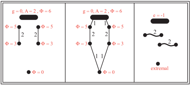
Figure 3.2. The decorated graph, extended graph and dull graph for a Hamiltonian circle action on a $4$-manifold.

3.3 Lemma.

For two Hamiltonian $S^{1}$-spaces of dimension four,

$$S^{1}\mathbin{\raisebox{-0.5pt}{\reflectbox{\begin{sideways}$\circlearrowleft$\end{sideways}}}}(M,\omega)\mbox{ and }S^{1}\mathbin{\raisebox{-0.5pt}{\reflectbox{\begin{sideways}$\circlearrowleft$\end{sideways}}}}(M^{\prime},\omega^{\prime}),$$

the following are equivalent.

1. The dull graphs of $M$ and $M^{\prime}$ are isomorphic as labelled graphs.

2. The extended decorated graphs of $M$ and $M^{\prime}$ with respect to a generic compatible metric differ by a composition of finitely many of the following maps:

   • the flip of the whole graph (plus a vertical translation);

   • the flip of a chain that begins and ends with an edge of label $1$; and

   • the positive rescaling of the lengths of the edges and of the area labels of the fat vertices that preserves the edge labels, the genus label, the $\mathrm{min}$ and $\mathrm{max}$ vertices and the corresponding $e_{\mathrm{min}}$ and $e_{\mathrm{max}}$, the adjacency relation, and the order by height of the vertices in each chain (plus a vertical translation).

We call a map in item (b) is a partial flip, as discussed in the Introduction. A map of type (c) is called a positive rescaling of the extended decorated graph. Note that the scaling factors can differ on each fat vertex and edge length. The effect of these maps in (a)-(c) are shown in Figure 3.4.

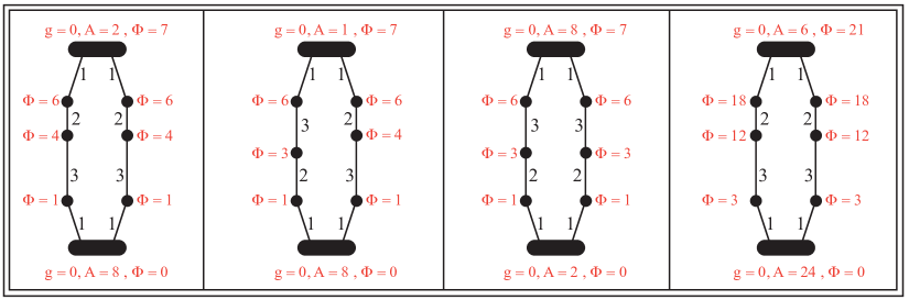
Figure 3.4. An extended decorated graph on the left; a partial flip of the extended graph; a full flip of the extended graph; and a (global) rescaling of the extended graph.

Proof.

The implication (2) $\Rightarrow$ (1) is straight forward because the dull graph simply forgets some of the information from the extended decorated graph. So the main content is to show (1) $\Rightarrow$ (2). Consider dull graphs that are obtained from the decorated graphs associated to Hamiltonian $S^{1}$-spaces of dimension four.

Recall that there are exactly two vertices that are either fat or labelled as extremal. By Proposition 2.4, the connected components of a dull graph are: the component of one extremal/fat vertex, the component of the other, (these two components might coincide), and (if exist) chains of edges in which all the vertices are interior. Note that such a chain might consist of a single isolated vertex, otherwise the endpoints are, each, on exactly one edge. In the extended decorated graph there might be an edge labelled one between an end-point of a chain and the $\mathrm{min}$ vertex and an edge labelled one between the other end-point and the $\mathrm{max}$ vertex.

An isomorphism of dull graphs preserves the extremal and fat vertices labels. So it sends the set of vertices that were $\mathrm{max}$ and $\mathrm{min}$ in the decorated graph of $S^{1}\mathbin{\raisebox{-0.5pt}{\reflectbox{\begin{sideways}$\circlearrowleft$\end{sideways}}}}(M,\omega)$ to the set of vertices that were $\mathrm{max}$ and $\mathrm{min}$ in the decorated graph of $S^{1}\mathbin{\raisebox{-0.5pt}{\reflectbox{\begin{sideways}$\circlearrowleft$\end{sideways}}}}(M^{\prime},\omega^{\prime})$. If it sends the vertex that was $\mathrm{max}$ to the vertex that was $\mathrm{max}$ and $\mathrm{min}$ to $\mathrm{min}$, then, on the vertices and edges of the connected components of the extremal vertices, it coincides with the map induced from the identity on the extended decorated graph. This can be seen by induction on the number of edges in the shortest path to an extremal vertex. Similarly, if it sends $\mathrm{max}$ to $\mathrm{min}$ and $\mathrm{min}$ to $\mathrm{max}$, then on the vertices and edges in the connected components of the extremal vertices, it coincides with the map induced from a flip of the extended decorated graph. When we say that maps coincide, it is always up to order of identical chains. In both cases, since the adjacency relation and the edge labels are preserved, on any other connected component, that is, a chain as described above, it coincides either with the map induced from the identity or with the map induced from a full flip of the extended decorated graph.

Now assume that the isomorphism of the dull graph is the identity map. Then the two extended graphs must agree on the type of the maximal (minimal) vertex (i.e., fat or isolated), and on its genus and self intersection when it is a fat vertex, and on the arrangement of the edges and their labels in each of the chains. Thus, up to chain flips of type (b), the extended graphs must differ by rescaling the heights of the moment map values and scaling the areas of the fat vertices, precisely a positive rescaling. Finally, we must verify that $e_{\mathrm{min}}$ and $e_{\mathrm{max}}$ are preserved. If the maximal vertex is fat then $e_{\mathrm{max}}$ is one of its labels in the dull graph hence does not change. If the maximal vertex is isolated then the number $e_{\mathrm{max}}$ in both decorated graphs is the reciprocal of the product of the labels adjacent to the vertex, hence it does not change. By the same argument, $e_{\mathrm{min}}$ does not change. This completes the proof. ∎

3.5 Remark.

If the decorated graphs of $(S^{1}\mathbin{\raisebox{-0.5pt}{\reflectbox{\begin{sideways}$\circlearrowleft$\end{sideways}}}}N,\omega_{N},\Phi_{N})$ and $(S^{1}\mathbin{\raisebox{-0.5pt}{\reflectbox{\begin{sideways}$\circlearrowleft$\end{sideways}}}}M,\omega_{M},\Phi_{M})$ differ by a map of type (a), then $S^{1}\mathbin{\raisebox{-0.5pt}{\reflectbox{\begin{sideways}$\circlearrowleft$\end{sideways}}}}N$ and $S^{1}\mathbin{\raisebox{-0.5pt}{\reflectbox{\begin{sideways}$\circlearrowleft$\end{sideways}}}}M$ are equivariantly diffeomorphic. To see that, we first note that equipping $M$ with $-\omega_{M}$ and the given $S^{1}$-action on $M$, we get a Hamiltonian $S^{1}$-manifold $(S^{1}\mathbin{\raisebox{-0.5pt}{\reflectbox{\begin{sideways}$\circlearrowleft$\end{sideways}}}}M,-\omega_{M},-\Phi_{M})$ whose decorated graph differ from the decorated graph of $(S^{1}\mathbin{\raisebox{-0.5pt}{\reflectbox{\begin{sideways}$\circlearrowleft$\end{sideways}}}}M,\omega_{M},\Phi_{M})$ by a map of type (a). By the uniqueness of the decorated graph [12, Theorem 4.1], $(S^{1}\mathbin{\raisebox{-0.5pt}{\reflectbox{\begin{sideways}$\circlearrowleft$\end{sideways}}}}M,-\omega_{M},-\Phi_{M})$ and $(S^{1}\mathbin{\raisebox{-0.5pt}{\reflectbox{\begin{sideways}$\circlearrowleft$\end{sideways}}}}N,\omega_{N},\Phi_{N})$ are equivariantly symplectomorphic, in particular $S^{1}\mathbin{\raisebox{-0.5pt}{\reflectbox{\begin{sideways}$\circlearrowleft$\end{sideways}}}}M$ and $S^{1}\mathbin{\raisebox{-0.5pt}{\reflectbox{\begin{sideways}$\circlearrowleft$\end{sideways}}}}N$ are equivariantly diffeomorphic.

We note that the decorated graph of $(S^{1}\mathbin{\raisebox{-0.5pt}{\reflectbox{\begin{sideways}$\circlearrowleft$\end{sideways}}}}N,\omega_{N},\Phi_{N})$ also coincides with that of the $S^{1}$-manifold obtained from $S^{1}\mathbin{\raisebox{-0.5pt}{\reflectbox{\begin{sideways}$\circlearrowleft$\end{sideways}}}}(M,\omega_{M})$ by precomposing with the non-trivial automorphism of the circle. Hence the map (a) also indicates a strictly weakly equivariant diffeomorphism.

A map of type (c) corresponds to an equivariant diffeomorphism as well. We will show that, geometrically, it corresponds to changing the sizes of the symplectic blowups, which changes the symplectic form on the resulting manifold but not the equivariant diffeomorphism type.

Let $M$ be a complex manifold obtained by $k$ complex blowups at $k$ distinct points from $M_{0}$ that is either ${\mathbb{C}}{\mathbb{P}}^{2}$, or $\operatorname{Hirz}_{N}$, or a ruled surface, i.e., an $S^{2}$-bundle over $(\Sigma,j)$ with a ruled integrable complex structure, with $g(\Sigma)>0$. A blowup form on $M$ is a symplectic form for which there exist disjoint embedded symplectic spheres (oriented by the symplectic form) in the homology classes

• $L,E_{1},\ldots,E_{k}$ if $M_{0}={\mathbb{C}}{\mathbb{P}}^{2}$;

• $S_{0},F_{0},E_{1},\ldots,E_{k}$ if $M_{0}$ is $\operatorname{Hirz}_{N}$;

• $F,E_{1},\ldots,E_{k}$ if $M_{0}$ is a ruled surface with $g(\Sigma)>0$.

We say that a diffeomorphism $M\to M^{\prime}$ is a positive rescaling of the blowup form $\omega$ if it pulls back $\omega^{\prime}$ to a blowup form obtained from $\omega$ by

• rescaling the sizes $\frac{1}{2\pi}\langle\omega,E_{i}\rangle$ for $i=1,\ldots,n$ and $\frac{1}{2\pi}\langle\omega,F\rangle$, $\frac{1}{2\pi}\langle\omega,B^{*}\rangle$, if $(M,\omega)$ is an $n$-fold blowup of a ruled surface and $B^{*}$ is as in (2.18);

• rescaling the sizes $\frac{1}{2\pi}\langle\omega,E_{i}\rangle$ for $i=1,\ldots,n$ and $\frac{1}{2\pi}\langle\omega,S_{0}\rangle$, $\frac{1}{2\pi}\langle\omega,F_{0}\rangle$, if $(M,\omega)$ is an $n$-fold blowup of a Hirzebruch surface; or

• rescaling the sizes $\frac{1}{2\pi}\langle\omega,E_{i}\rangle$ for $i=1,\ldots,n$ and $\frac{1}{2\pi}\langle\omega,L\rangle$, if $(M,\omega)$ is an $n$-fold blowup of ${\mathbb{C}}{\mathbb{P}}^{2}$.

3.6 Proposition.

The extended decorated graphs of $S^{1}\mathbin{\raisebox{-0.5pt}{\reflectbox{\begin{sideways}$\circlearrowleft$\end{sideways}}}}(M,\omega)$ and $S^{1}\mathbin{\raisebox{-0.5pt}{\reflectbox{\begin{sideways}$\circlearrowleft$\end{sideways}}}}(M^{\prime},\omega^{\prime})$ (w.r.t. generic compatible metrics) differ by a positive rescaling if and only if there is an equivariant diffeomorphism $(M,\omega)\to(M^{\prime},\omega^{\prime})$ that is a positive rescaling of the blowup form.

Proof.

The $\Leftarrow$ implication is straight forward. To prove the other direction, we proceed by induction on the sum $\ell$ of the number of fat vertices and the number of edges in the extended graph. Our base cases are the minimal models and have $\ell=3,4$.

If $\ell=3$ then, by the minimal models §2.24 and the effect of a blowup §2.19, we must have $(M,\omega)=({\mathbb{C}}{\mathbb{P}}^{2},\lambda\omega_{\text{FS}})$ and the extended decorated graph of the circle action is (up to a flip) either (b) or (c) in Figure 2.13. In (b), the area label of the fat vertex and the lengths of the edges are all equal. In (c), dividing the edge-length by the edge-label gives the same result for all three edges. If a positive rescaling of the edge-lengths and area label yields the graph of a Hamiltonian $S^{1}\mathbin{\raisebox{-0.5pt}{\reflectbox{\begin{sideways}$\circlearrowleft$\end{sideways}}}}(M^{\prime},\omega^{\prime})$ then the obtained graph will be again as in (b) or (c) in Figure 2.13, respectively, and the scaling of all the edge-lengths and labels would be by the same factor. By uniqueness of the decorated graph [12, Theorem 4.1], $S^{1}\mathbin{\raisebox{-0.5pt}{\reflectbox{\begin{sideways}$\circlearrowleft$\end{sideways}}}}(M^{\prime},\omega^{\prime})$ is equivariantly symplectomorphic to $S^{1}\mathbin{\raisebox{-0.5pt}{\reflectbox{\begin{sideways}$\circlearrowleft$\end{sideways}}}}({\mathbb{C}}{\mathbb{P}}^{2},\lambda^{\prime}\omega_{\text{FS}})$. Since $\lambda$ ($\lambda^{\prime}$) is $\frac{1}{2\pi}$ the area of the line ${\mathbb{C}}{\mathbb{P}}^{1}$ in $L$, it equals the area label of the fat vertex if the rescaled graph is (b), and the edge-length over the edge-label for each of the edges if the rescaled graph is (c). In both cases, the positive rescaling of the graph corresponds to the positive rescaling $\lambda\mapsto\lambda^{\prime}$ of the blowup form.

If $\ell=4$, then by §2.24, $(M,\omega)$ is a symplectic ruled surface, either rational or irrational. In the first case $(M,\omega)$ is a Hirzebruch surface $(\operatorname{Hirz}_{N},\eta_{\beta,f})$. If $N=1$, it is also a blowup of ${\mathbb{C}}{\mathbb{P}}^{2}$ at one point. The extended decorated graph for the circle action is thus one of the graphs in Figure 2.16. In the second case, $S^{1}\mathbin{\raisebox{-0.5pt}{\reflectbox{\begin{sideways}$\circlearrowleft$\end{sideways}}}}(M,\omega)$ is a symplectic $S^{1}$-ruled surface of positive genus and its extended decorated graph is as in (a) in Figure 2.16 with the $g>0$. The symplectic size of the fiber at zero $F_{0}$ (respectively, the fiber $F$) is $2\pi$ times

$$\begin{cases}\text{the length of each edge}&\text{ in (a) }\\ \left[\text{\begin{tabular}[]{l}the area label of the fat vertex =\\ $\frac{1}{N}$(the length of the $N$-labelled edge)\end{tabular}}\right.&\text{ in (b) }\\ \frac{1}{n}(\text{the length of the $n$-labelled edge})&\text{ in (c) }\\ \frac{1}{n}(\text{the length of the $n$-labelled edge})&\text{ in (d) }\end{cases},$$

and the symplectic size of the zero section $S_{0}$ (respectively, the base $B^{*}$) is $2\pi$ times

$$\begin{cases}\text{the area label of the min fat vertex }+\frac{e_{\mathrm{max}}}{2}(\text{the fiber size})&\text{ in (a) }\\ \frac{1}{2}(\text{the length of the left edge})+\frac{1}{2}(\text{ the length of the $N$-labelled edge})&\text{ in (b) }\\ \frac{1}{m}(\text{the length of the left $m$ edge})+\frac{1}{2m^{2}}\left(\frac{1}{e_{\mathrm{max}}}-\frac{1}{e_{\mathrm{min}}}\right)(\text{the fiber size})&\text{ in (c) }\\ \frac{1}{m}(\text{the length of the left $m$ edge})+\frac{1}{2m^{2}}\left(\frac{1}{e_{\mathrm{max}}}-\frac{1}{e_{\mathrm{min}}}\right)(\text{the fiber size})&\text{ in (d) }\end{cases}.$$

Note that $N$ is determined by the edge labels in the decorated graph and the labels $e_{\mathrm{max}}$ and $e_{\mathrm{min}}$: it is $e_{\mathrm{min}}$ in (a), the label of an edge in (b), $\frac{1}{2m^{2}}\left(\frac{1}{e_{\mathrm{max}}}-\frac{1}{e_{\mathrm{min}}}\right)$ (where $m$ is the duplicate label) in (d) and (c). So $N$ is not affected by a positive rescaling of the graph. Also note that the edge-lengths of the remaining edges and the area label of the remaining fat vertex are determined by the above sizes and by equations (2.6) and (2.7). If the graph obtained by a positive rescaling is the extended (generic) decorated graph of a Hamiltonian $S^{1}\mathbin{\raisebox{-0.5pt}{\reflectbox{\begin{sideways}$\circlearrowleft$\end{sideways}}}}(M^{\prime},\omega^{\prime})$ then the rescaled graph is again as in Figure 2.16, respectively, with the same $N$ and with $\beta^{\prime},f^{\prime}$ obtained by a positive rescaling of $\beta$ and $f$.

For the induction step, Let $S^{1}\mathbin{\raisebox{-0.5pt}{\reflectbox{\begin{sideways}$\circlearrowleft$\end{sideways}}}}M$ with $\ell\geq 5$. By the list of minimal models §2.24 and the blowup process §2.19, there is a compatible integrable complex structure $J$ such that $S^{1}\mathbin{\raisebox{-0.5pt}{\reflectbox{\begin{sideways}$\circlearrowleft$\end{sideways}}}}(M,\omega,J)$ is obtained by a single equivariant Kähler blowup from $S^{1}\mathbin{\raisebox{-0.5pt}{\reflectbox{\begin{sideways}$\circlearrowleft$\end{sideways}}}}(\overline{M},\overline{\omega},\overline{J})$ (with $\ell$ now one less) and the image of the exceptional divisor under the moment map is either a fat $\mathrm{min}$-vertex, a fat $\mathrm{max}$-vertex, or a non-ephemeral edge in the extended (generic) decorated graph. In the first two cases, the label $e_{\mathrm{min}/\mathrm{max}}$ is $-1$ and the genus label $g$ is $0$. In the third case, if the edge is the $j^{\mathrm{th}}$ from the bottom on the $i^{\mathrm{th}}$ chain, then by §6.28, the combinatorial intersection number $\frac{m_{i,j-1}-m_{i,j+1}}{m_{i,j}}$ equals $-1$. Recall that here $m_{i,k}$ is the label of the $k^{\mathrm{th}}$ edge in the $i^{\mathrm{th}}$ chain for $1\leq k\leq\ell_{i}$, and $m_{i,0},m_{i,\ell_{i+1}}$ are as in (4.17) and (4.18).

The rescaling doesn’t change the $e_{\mathrm{min}/\mathrm{max}}$, $g$, the $m_{i,k}$ labels, the adjacency relation, or the thickness of the extremal vertices. So the extended decorated graph of $(M^{\prime},\omega^{\prime})$ also contains a fat vertex or edge, respectively, with the same $e_{\mathrm{min}/\mathrm{max}}$ and $g$ labels and combinatorial intersection numbers. Moreover, because each graph is determined with respect to a generic metric, Proposition 2.27 guarantees that if the exceptional divisor corresponds to an edge, it is non-ephemeral. It is the image under the moment map of an embedded invariant complex (and symplectic) sphere, complex with respect to a compatible integrable complex structure $J^{\prime}$ on $S^{1}\mathbin{\raisebox{-0.5pt}{\reflectbox{\begin{sideways}$\circlearrowleft$\end{sideways}}}}(M^{\prime},\omega^{\prime})$. The preimage of a fat vertex is also such a sphere; see Remark 2.25. Note that the symplectic areas of the corresponding complex spheres in $(M,\omega,J)$ and in $(M^{\prime},\omega^{\prime},J^{\prime})$ might differ by a positive factor. Blowing down equivariantly, along the corresponding embedded complex spheres in $S^{1}\mathbin{\raisebox{-0.5pt}{\reflectbox{\begin{sideways}$\circlearrowleft$\end{sideways}}}}(M,\omega,J)$ and in $S^{1}\mathbin{\raisebox{-0.5pt}{\reflectbox{\begin{sideways}$\circlearrowleft$\end{sideways}}}}(M^{\prime},\omega^{\prime},J^{\prime})$ yields decorated graphs that differ, again, by a positive rescaling. By the induction hypothesis, the blown down $(\overline{M},\overline{\omega})$ and $(\overline{M^{\prime}},\overline{\omega^{\prime}})$ are $S^{1}$-equivariantly diffeomorphic by a positive rescaling of the blowup form. Thus, we deduce that $(M,\omega)$ and $(M^{\prime},\omega^{\prime})$ are $S^{1}$-equivariantly diffeomorphic by a positive rescaling of the blowup form, completing the proof. ∎

4. A Generators-and-Relations description:
Notation, statements and corollaries

The goal of this section is to give a generators and relations presentation for the equivariant cohomology of a Hamiltonian circle action on a closed symplectic manifold of dimension four, as a module over $H_{S^{1}}^{*}(\operatorname{pt})$. The odd-degree part plays only a minor role, so we begin by analyzing $H_{S^{1}}^{2*}(M;{\mathbb{Z}})$.

Even degree equivariant cohomology

4.1 Notation (The Generators).

Let $S^{1}\mathbin{\raisebox{-0.5pt}{\reflectbox{\begin{sideways}$\circlearrowleft$\end{sideways}}}}M^{4}$ be a closed symplectic $4$-manifold equipped with a Hamiltonian circle action. Consider the associated extended decorated graph with respect to a generic compatible Kähler metric. Suppose that the extended decorated graph for $S^{1}\mathbin{\raisebox{-0.5pt}{\reflectbox{\begin{sideways}$\circlearrowleft$\end{sideways}}}}M^{4}$ consists of $k$ chains $C_{1},\dots,C_{k}$ of edges between the maximum and minimum vertices. Note that $k\geq 2$, by our conventions in 2.3 If there are no fixed surfaces then the number of chains $k=2$. For each chain $1\leq i\leq k$, let $\ell_{i}$ be the number of edges in the chain $C_{i}$; we enumerate the edges on $C_{i}$ by their order in the chain, starting from the bottom. Denote by $m_{i,j}$ the label of the $(i,j)$ edge. Without loss of generality, we assume that if there is exactly one fat vertex then it is maximal. We assume that the chains are ordered such that $m_{1,1}\geq m_{2,1}\geq\cdots\geq m_{k,1}$.

If the minimal vertex is fat denote its moment-map preimage by $\Sigma_{0}$. If the maximal vertex is fat denote its preimage by $\Sigma_{\infty}$. If the $j^{\mathrm{th}}$ edge on the $i^{\mathrm{th}}$ chain is non-ephemeral we denote by $S_{i,j}$ the $S^{1}$-invariant embedded symplectic sphere whose moment map image is the edge; such a sphere exists if $1<j\leq\ell_{k}$ for all $i$, if $j=1$ for all $i$ if $\sharp\text{fat vertices}=0\text{ or }2$, and if $j=1$ and $\sharp\text{fat vertices}=1$ for $i$ such that $m_{i,1}\geq m_{2,1}$ (see Proposition 2.27). By Remark 2.25, each of the preimages $\Sigma_{0},\Sigma_{\infty}$ is an invariant embedded symplectic surface, and the $S_{i,j}$s are well defined. If $m_{i,j}>1$ the sphere $S_{i,j}$ is a ${\mathbb{Z}}_{m_{i,j}}$-sphere. Every two distinct spheres $S_{i,j},\neq S_{i^{\prime},j^{\prime}}$ are either disjoint or intersect at a single isolated fixed point.

We define the following the degree $2$ classes

$$\tau_{0}:=\iota_{\Sigma_{0}}^{!}(\mathbb{1}),\,\,\tau_{\infty}:=\iota_{\Sigma_{\infty}}^{!}(\mathbb{1}),\,\,\sigma_{i,j}:=\iota_{S_{i,j}}^{!}(\mathbb{1}).$$

If $\Sigma_{0}$ ($\Sigma_{\infty}$) does not exist, we set $\tau_{0}=0$ ($\tau_{\infty}=0$).

In a graph with two fat vertices and zero isolated vertices, corresponding to an $S^{1}$-ruled symplectic $S^{2}$-bundle over a closed surface, let $\tau_{h}:=\iota_{S}^{!}(\mathbb{1})$ where $S$ in an invariant embedded symplectic sphere in the fiber class. Note that in this case $\sigma_{1,1}=\tau_{h}=\sigma_{2,1}$ and $m_{1,1}=1=m_{2,1}$. Otherwise, denote

$$\tau_{h}:=\sum_{j=1}^{\ell_{1}}m_{1,j}\sigma_{1,j}.$$

In a graph with exactly one fat vertex, if the first edge in the $i^{\mathrm{th}}$ chain is ephemeral, denote

$$\sigma_{i,1}:=\tau_{h}-\sum_{j=2}^{\ell_{i}}m_{i,j}\sigma_{i,j}.$$

Denote by $\mathrm{max}$ ($\mathrm{min}$) the fixed component of maximal (minimal) value of the moment map, it can be either a fixed surface $\Sigma_{\infty}$ ($\Sigma_{0}$) or an isolated vertex $v_{\infty}$ ($v_{0}$).

For $1\leq i\leq k$ and $1\leq j<\ell_{i}$ denote by $v_{i,j}$ the south pole of the $S^{1}$-invariant embedded symplectic sphere $S_{i,j+1}$ whose moment map image is the $(i,j+1)$ edge in the extended decorated graph, i.e., the point on $S_{i,j+1}$ that is of minimal moment map value. We use the same notation $v_{i,j}$ for the corresponding (isolated) vertex of the decorated graph.

4.2 Notation (The Relations).

There are two types of relations among the generators defined above, multiplicative relations and linear relations.

The multiplicative relations can be verified using localization. They hold because the submanifolds that are Poincaré dual to the classes can be chosen to be disjoint. We define the multiplicative ideal $\mathcal{I}$ to be generated by

1. $\tau_{0}\cup\tau_{\infty}$

2. $\tau_{0}\cup\sigma_{i,j}$ for every $2\leq j\leq\ell_{i}$

3. $\tau_{\infty}\cup\sigma_{i,j}$ for every $1\leq j\leq\ell_{i}-1$

4. $\sigma_{i,j}\cup\sigma_{m,n}$ whenever we can choose the spheres so that $S_{i,j}\cap S_{m,n}=\emptyset$

5. $\tau_{h}^{2}$ when there is both a fat minimum and fat maximum

6. $\tau_{\infty}\cup\sigma_{1,1}\cup\sigma_{2,1}$ when $M={\mathbb{C}}{\mathbb{P}}^{2}$ and there is a fat vertex

7. $\sigma_{1,1}\cup\sigma_{2,1}\cup\sigma_{2,2}$ when $M={\mathbb{C}}{\mathbb{P}}^{2}$ and there is no fat vertex

For item A, this is redundant when there are not two fat vertices. For items of type B, these are redundant if there is no fat minimum or no fat maximum, respectively. Items of type D apply for special cases as indicated. Finally, for item C, we note that we can choose the spheres so that $S_{i,j}\cap S_{m,n}=\emptyset$ whenever

• $i=m$ and $|j-n|\geq 2$;

• $i\neq m$ and both $1<j<\ell_{i}$, $1<n<\ell_{m}$;

• $i\neq m$, $j=1<\ell_{i}$, and $1<\ell_{m}=n$;

• the minimum is fat, $i\neq m$, and $j=n=1$; or

• the maximum is fat, $i\neq m$, $j=\ell_{i}$, and $n=\ell_{m}$.

The reader familiar with toric varieties will recognize this type of relation. The condition that we can choose the spheres so that $S_{i,j}\cap S_{m,n}=\emptyset$ is equivalent to the condition that the corresponding edges in the extended graph are disjoint.

The linear relations can also be verified by localization. We define the linear relation ideal to be

$$\mathcal{J}=\left\langle\tau_{h}-\sum_{j=1}^{\ell_{i}}m_{i,j}\sigma_{i,j}\ \ \ \forall\ 1\leq i\leq k\right\rangle.$$

If the action $S^{1}\mathbin{\raisebox{-0.5pt}{\reflectbox{\begin{sideways}$\circlearrowleft$\end{sideways}}}}M$ extends to a toric $T^{2}\mathbin{\raisebox{-0.5pt}{\reflectbox{\begin{sideways}$\circlearrowleft$\end{sideways}}}}M$, the reader familiar with toric varieties will recognize these relations as part of a linear system on the $T^{2}$-equivariant cohomology of $M$. A full linear system describe the kernel of the restriction map from $T^{2}$-equivariant to ordinary cohomology. In this case, $\mathcal{J}$ describe the difference between the $T^{2}$- and $S^{1}$-equivariant cohomology rings:

$$H_{T^{2}}^{*}(M;{\mathbb{Z}})/\mathcal{J}\cong H_{S^{1}}^{*}(M;{\mathbb{Z}}).$$

We are now prepared to state our main theorem describing $H_{S^{1}}^{2*}(M;{\mathbb{Z}})$ by generators and relations.

4.3 Theorem.

Let $M$ be a compact symplectic $4$-manifold endowed with a Hamiltonian $S^{1}$ action. Then

$$H_{S^{1}}^{2*}(M;{\mathbb{Z}}) = \frac{{\mathbb{Z}}[\tau_{0},\tau_{\infty},\tau_{h},\sigma_{1,1},\dots,\sigma_{1,\ell_{1}},\dots,\sigma_{k,1},\dots,\sigma_{k,\ell_{k}}]}{\mathcal{I}+\mathcal{J}}.$$

Moreover, the map $\pi^{*}:H_{S^{1}}^{*}(pt;{\mathbb{Z}})\to H_{S^{1}}^{2*}(M;{\mathbb{Z}})$ endows $H_{S^{1}}^{2*}(M;{\mathbb{Z}})$ with the structure of an $H_{S^{1}}^{*}(pt;{\mathbb{Z}})$-module. This structure is determined by the image of the generator

(4.4) $${}\pi^{*}(t)=\tau_{\infty}-\tau_{0}+(\Sigma_{0}\cdot\Sigma_{0})\tau_{h}+\sum_{i=1}^{k}\sum_{j=1}^{\ell_{i}}b_{i,j}\sigma_{i,j},$$

where the $b_{i,j}$s are integers satisfying the properties listed in Lemma 4.5 below.

We note that we can omit the $\sigma_{i,j}$s that correspond to ephemeral edges from the list of generators, and moreover omit $\sigma_{i,1}$ for $i\geq 3$ in general, since they are linear combinations of the other $\sigma_{i,j}$s over ${\mathbb{Z}}$. Some of the listed generators might be the zero element: $\tau_{\infty}$ if $\sharp\text{fat vertices}=0$; $\tau_{0}$ if $\sharp\text{fat vertices}<2$.

4.5 Lemma.

For $1\leq i\leq k$ and $1\leq j\leq\ell_{i}$, there are integers $b_{i,j}$ so that for $j\geq 2$,

(4.6) $$b_{i,j}m_{i,j-1}-b_{i,j-1}m_{i,j}=1.$$

The $b_{i,j}$s are determined recursively once we fix $b_{i,1},\,b_{i,2}$ satisfying $b_{i,2}m_{1}-b_{i,1}m_{2}=1$. We can furthermore set the $b_{i,j}$s such that if there is a maximal fixed surface then

(4.7) $$\Sigma_{\infty}\cdot\Sigma_{\infty}+\Sigma_{0}\cdot\Sigma_{0}+\sum_{i=1}^{k}b_{i,\ell_{i}}=0,$$

and if there is, in addition, a minimal fixed surface then

(4.8) $$\sum_{i=1}^{k}b_{i,1}=0.$$

Moreover, we can set the $b_{i,j}$s such that they have the following additional properties depending on the nature of the dull graph.

• Assume that there are two fixed surfaces. We can choose $b_{i,1}=0$. For $\ell_{i}>1$ we can choose $b_{i,2}=1$; we then have $b_{i,\ell_{i}}=1$.

• Assume that there are no fixed surfaces (hence $k=2$). We can choose the $b_{i,j}$s such that they satisfy the gcd relation cyclically, i.e.,

  $$-b_{1,1}m_{2,1}-b_{2,1}m_{1,1}=1\mbox{ and }b_{2,\ell_{2}}m_{1,\ell_{1}}+b_{1,\ell_{1}}m_{2,\ell_{2}}=1.$$

  Moreover, if $m_{1,\ell_{1}}=1=m_{2,\ell_{2}}$ we can choose $b_{1,\ell_{1}}=0$ and $b_{2,\ell_{2}}=1$, such that if $\ell_{i}=1$ then $b_{i,\ell_{i}}=0$. Alternatively, if $m_{1,1}=1=m_{2,1}$ we can choose $b_{1,1}=0$ and $b_{2,1}=-1$, such that if $\ell_{i}=1$ then $b_{i,1}=0$. Note that we might not be able to make the latter two choices simultaneously.

• Assume that there is exactly one fixed surface. By convention, it is maximal and the chains are ordered such that $m_{1,1}\geq m_{2,1}\geq 1=m_{3,1}=\cdots=m_{k,1}$. If $\ell_{i}\geq 2$ for some $i$, we may choose the $b_{i,j}$s in the first two chains so that the cyclic gcd relation

  $$-b_{1,1}m_{2,1}-b_{2,1}m_{1,1}=1$$

  is satisfied. For the remaining $k-2$ chains we may choose $b_{i,1}=0,\,b_{i,2}=1$, which yields $b_{i,\ell_{i}}=1$ as in the two-surface case. If $k=2$ and $\ell_{1}=\ell_{2}=1$, then we set $b_{1,1}=0$ and $b_{2,1}=-1$.

Proof.

The existence of integers $b_{i,j}$s that satisfy the basic property (4.6) is proved in [12, Lemma 5.7]; we include the proof here for completeness. To prove that we can set the $b_{i,j}$s such that (4.6), (4.7), (4.8) hold, and verify items (a), (b) and (c), we apply straight forward induction arguments.

Base Case: The minimal models.

Figure 4.9. The base cases.

In Figure 4.9, the $m_{i,j}$ are marked in black and the $b_{i,j}$ are marked in red for the possible labeled graphs for $S^{1}\mathbin{\raisebox{-0.5pt}{\reflectbox{\begin{sideways}$\circlearrowleft$\end{sideways}}}}M$. Since $m$ and $n$ are relatively prime, we have fixed $a,b\in{\mathbb{Z}}$ such that $am-bn=1$ as in (2.10). We have also indicated in blue the self intersections of the fat vertices. The self intersections are calculated using §2.5 , Figures 2.13 and 2.16, and Notation 2.17. It is then straight-forward to show that the relations (4.6), (4.7), (4.8), and (a), (b), and (c) hold for the minimal models. For example, Figure 4.9(ii), for the length two chain, we verify (4.6) by

$$(a-b)\cdot n-(-a)\cdot(m-n)=an-bn+am-an=am-bn=1;$$

for the cyclic relation of part (b) of the Lemma, around the top, we have

$$(a-b)\cdot m+b\cdot(m-n)=am-bm+bm-bn=am-bn=1;$$

and for the cyclic relation of part (b) of the Lemma, around the bottom

$$-b\cdot n-(-a)\cdot m=am-bn=1.$$

Inductive Step. The effect of a blowup, by type. In each case, the old and new $m_{i,j}$, $b_{i,j}$ and self intersection of a fat vertex are marked in black, red and blue respectively.

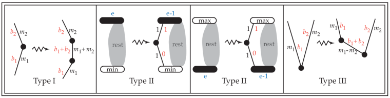
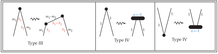
Figure 4.10. The inductive step. In the last figure, we must be careful to flip if there was not a fat vertex at the top, and reassign the $b_{i,j}$s according to our convention.

Again, straight forward computations show that the properties (4.6), (4.7), (4.8), (a), (b) and (c) are maintained. For example, in Type I we assume by induction that

$$b_{2}m_{1}-b_{1}m_{2}=1$$

which then lets us deduce that

$$b_{2}\cdot(m_{1}+m_{2})-(b_{1}+b_{2})\cdot m_{2}=b_{2}m_{1}+b_{2}m_{2}-b_{1}m_{2}-b_{2}m_{2}=b_{2}m_{1}-b_{1}m_{2}=1,$$

and similarly

$$(b_{1}+b_{2})\cdot m_{1}-b_{1}\cdot(m_{1}+m_{2})=b_{1}m_{1}+b_{2}m_{1}-b_{1}m_{1}-b_{1}m_{2}=b_{2}m_{1}-b_{1}m_{2}=1.$$

One must be careful when introducing a fat vertex in a blowup of Type IV. In case the fat vertex introduced at the blowup is the first one, and is maximal, we set $b_{1,\ell_{1}}=0$ and $b_{2,\ell_{2}}=1$, such that if $\ell_{i}=1$ then $b_{i,\ell_{i}}=0$, at the left graph (before the blowup); the blowup has no effect then on the $b_{i,j}$s, and in particular $b_{1,\ell_{1}}=0$ and $b_{2,\ell_{2}}=1$ at the right graph as well. In case a second fat vertex is introduced at the blowup, one may need to re-define all of the $b_{i,j}$ because what results from the cyclic convention does not agree with the convention described in (a). Again, one can argue inductively: once there are two fixed surfaces, it is possible to equivariantly blow down to a minimal model with two fixed surfaces [12, Lemma C.14], and re-start the inductive process from that minimal model, using only blowups of Types I and II. This completes the inductive step.

It is also possible to prove (b) directly, the case where there are isolated fixed points. Indeed, here the action must extend to a toric one, with the circle action corresponding to $\begin{bmatrix}m\\ n\end{bmatrix}$. Again, we have fixed $a$ and $b$ so that $am-bn=1$ as in (2.10). The $m_{i,j}$ and $b_{i,j}$ can now be defined in terms of the toric action. To see this, we let $e_{1},\dots,e_{L}$ be the vectors parallel to the edges of the toric polygon, as in Figure 4.11(i).

Figure 4.11. In (i) is Delzant polytope with edge directions $e_{i}$ marked as red vectors. In (ii), (ii) and (iv) are the labelled graphs for three different choices of $\left(\begin{array}[]{cc}m\\ n\end{array}\right)$. with isotropy labels $m_{i,j}$ in black and $b_{i,j}$ in red.

Define

$$\mu_{i}=\left\langle\begin{bmatrix}m\\ n\end{bmatrix},e_{i}\right\rangle\mbox{ and }\beta_{i}=\left\langle\begin{bmatrix}b\\ a\end{bmatrix},e_{i}\right\rangle.$$

That the circle action corresponding to $\begin{bmatrix}m\\ n\end{bmatrix}$ has isolated fixed points means that no $\mu_{i}=0$. We check that

$$\beta_{i+1}\mu_{i}-\beta_{i}\mu_{i+1} = \left\langle\begin{bmatrix}b\\ a\end{bmatrix},e_{i+1}\right\rangle\cdot\left\langle\begin{bmatrix}m\\ n\end{bmatrix},e_{i}\right\rangle-\left\langle\begin{bmatrix}b\\ a\end{bmatrix},e_{i}\right\rangle\cdot\left\langle\begin{bmatrix}m\\ n\end{bmatrix},e_{i+1}\right\rangle$$

$$= \det\left(\begin{bmatrix}m&n\\ b&a\\ \end{bmatrix}\cdot\begin{bmatrix}\top&\top\\ e_{i}&e_{i+1}\\ \bot&\bot\end{bmatrix}\right)$$

$$= \det\left(\begin{bmatrix}m&n\\ b&a\\ \end{bmatrix}\right)\cdot\det\left(\begin{bmatrix}\top&\top\\ e_{i}&e_{i+1}\\ \bot&\bot\end{bmatrix}\right)=1\cdot 1.$$

This wraps around modulo $L$ where $L=\ell_{1}+\ell_{2}$ is the number of edges in the polygon.

We note that $\mu_{i}>0$ on one chain and $\mu_{i}<0$ on the other chain. The labels $m_{i,j}$ then correspond precisely to the appropriate $|\mu_{k}|$. The $b_{i,j}$ are exactly $\beta_{k}$. One then has to carefully check that the sign changes exactly cancel out and the relations described in (b) continue to hold. ∎

4.12.

Localization in equivariant cohomology. By [11, Theorem 1.1(A)] the inclusion of the fixed point components

$$i=\bigoplus_{F\subset M^{S^{1}}}\iota_{F}\colon M^{S^{1}}\hookrightarrow M$$

induces an injection in equivariant cohomology

$$i^{*}\colon H_{S^{1}}^{*}(M;{\mathbb{Z}})\hookrightarrow H_{S^{1}}^{*}(M^{S^{1}};{\mathbb{Z}})=\bigoplus_{F\subset M^{S^{1}}}H^{*}(F)\otimes{\mathbb{Z}}[t].$$

Let $F$ be a connected component of the fixed point set $M^{S^{1}}$. Let $X$ be an invariant embedded symplectic (oriented) sphere in $S^{1}\mathbin{\raisebox{-0.5pt}{\reflectbox{\begin{sideways}$\circlearrowleft$\end{sideways}}}}(M,\omega)$, and $\eta=\iota^{!}_{X\hookrightarrow M}(\mathbb{1}_{X})$. Consider the following diagram of inclusion maps:

(4.13) $${}\begin{array}[]{c}\lx@xy@svg{\hbox{\raise 0.0pt\hbox{\kern 24.52754pt\hbox{\ignorespaces\ignorespaces\ignorespaces\hbox{\vtop{\kern 0.0pt\offinterlineskip\halign{\entry@#!@&&\entry@@#!@\cr&&\\&&\crcr}}}\ignorespaces{\hbox{\kern-16.99995pt\raise 0.0pt\hbox{\hbox{\kern 0.0pt\raise 0.0pt\hbox{\hbox{\kern 3.0pt\raise 0.0pt\hbox{$\textstyle{F\cap X\ignorespaces\ignorespaces\ignorespaces\ignorespaces\ignorespaces\ignorespaces\ignorespaces\ignorespaces}$}}}}}}}\ignorespaces\ignorespaces\ignorespaces\ignorespaces{}{\hbox{\lx@xy@droprule}}\ignorespaces\ignorespaces\ignorespaces{\hbox{\kern 29.62857pt\raise 5.60695pt\hbox{{}\hbox{\kern 0.0pt\raise 0.0pt\hbox{\hbox{\kern 3.0pt\hbox{\hbox{\kern 0.0pt\raise-0.40695pt\hbox{$\scriptstyle{\iota_{F\cap X\hookrightarrow F}}$}}}\kern 3.0pt}}}}}}\ignorespaces{\hbox{\kern 76.37494pt\raise 0.0pt\hbox{\hbox{\kern 0.0pt\raise 0.0pt\hbox{\lx@xy@tip{1}\lx@xy@tip{-1}}}}}}{\hbox{\lx@xy@droprule}}{\hbox{\lx@xy@droprule}}\ignorespaces\ignorespaces\ignorespaces\ignorespaces{}{\hbox{\lx@xy@droprule}}\ignorespaces\ignorespaces\ignorespaces{\hbox{\kern-24.52754pt\raise-18.41666pt\hbox{{}\hbox{\kern 0.0pt\raise 0.0pt\hbox{\hbox{\kern 3.0pt\hbox{\hbox{\kern 0.0pt\raise-0.40695pt\hbox{$\scriptstyle{\iota_{F\cap X\hookrightarrow X}}$}}}\kern 3.0pt}}}}}}\ignorespaces{\hbox{\kern 0.0pt\raise-27.0pt\hbox{\hbox{\kern 0.0pt\raise 0.0pt\hbox{\lx@xy@tip{1}\lx@xy@tip{-1}}}}}}{\hbox{\lx@xy@droprule}}{\hbox{\lx@xy@droprule}}{\hbox{\kern 40.99995pt\raise 0.0pt\hbox{\hbox{\kern 0.0pt\raise 0.0pt\hbox{\hbox{\kern 3.0pt\raise 0.0pt\hbox{$\textstyle{{\color[rgb]{1,1,1}.}}$}}}}}}}{\hbox{\kern 76.37494pt\raise 0.0pt\hbox{\hbox{\kern 0.0pt\raise 0.0pt\hbox{\hbox{\kern 3.0pt\raise 0.0pt\hbox{$\textstyle{F\ignorespaces\ignorespaces\ignorespaces\ignorespaces}$}}}}}}}\ignorespaces\ignorespaces\ignorespaces\ignorespaces{}{\hbox{\lx@xy@droprule}}\ignorespaces\ignorespaces\ignorespaces{\hbox{\kern 83.28467pt\raise-18.41666pt\hbox{{}\hbox{\kern 0.0pt\raise 0.0pt\hbox{\hbox{\kern 3.0pt\hbox{\hbox{\kern 0.0pt\raise-0.40695pt\hbox{$\scriptstyle{\iota_{F\hookrightarrow M}}$}}}\kern 3.0pt}}}}}}\ignorespaces{\hbox{\kern 83.28467pt\raise-27.0pt\hbox{\hbox{\kern 0.0pt\raise 0.0pt\hbox{\lx@xy@tip{1}\lx@xy@tip{-1}}}}}}{\hbox{\lx@xy@droprule}}{\hbox{\lx@xy@droprule}}{\hbox{\kern-7.53471pt\raise-36.83331pt\hbox{\hbox{\kern 0.0pt\raise 0.0pt\hbox{\hbox{\kern 3.0pt\raise 0.0pt\hbox{$\textstyle{X\ignorespaces\ignorespaces\ignorespaces\ignorespaces}$}}}}}}}\ignorespaces\ignorespaces\ignorespaces\ignorespaces{}{\hbox{\lx@xy@droprule}}\ignorespaces\ignorespaces\ignorespaces{\hbox{\kern 31.93135pt\raise-42.44025pt\hbox{{}\hbox{\kern 0.0pt\raise 0.0pt\hbox{\hbox{\kern 3.0pt\hbox{\hbox{\kern 0.0pt\raise-0.40695pt\hbox{$\scriptstyle{\iota_{X\hookrightarrow M}}$}}}\kern 3.0pt}}}}}}\ignorespaces{\hbox{\kern 73.77773pt\raise-36.83331pt\hbox{\hbox{\kern 0.0pt\raise 0.0pt\hbox{\lx@xy@tip{1}\lx@xy@tip{-1}}}}}}{\hbox{\lx@xy@droprule}}{\hbox{\lx@xy@droprule}}{\hbox{\kern 40.99995pt\raise-36.83331pt\hbox{\hbox{\kern 0.0pt\raise 0.0pt\hbox{\hbox{\kern 3.0pt\raise 0.0pt\hbox{$\textstyle{{\color[rgb]{1,1,1}.}}$}}}}}}}{\hbox{\kern 73.77773pt\raise-36.83331pt\hbox{\hbox{\kern 0.0pt\raise 0.0pt\hbox{\hbox{\kern 3.0pt\raise 0.0pt\hbox{$\textstyle{M.}$}}}}}}}\ignorespaces}}}}\ignorespaces\end{array} \textstyle{F\cap X\ignorespaces\ignorespaces\ignorespaces\ignorespaces\ignorespaces\ignorespaces\ignorespaces\ignorespaces} \scriptstyle{\iota_{F\cap X\hookrightarrow F}} \scriptstyle{\iota_{F\cap X\hookrightarrow X}} \textstyle{F\ignorespaces\ignorespaces\ignorespaces\ignorespaces} \scriptstyle{\iota_{F\hookrightarrow M}} \textstyle{X\ignorespaces\ignorespaces\ignorespaces\ignorespaces} \scriptstyle{\iota_{X\hookrightarrow M}} \textstyle{M.} \textstyle{F\cap X\ignorespaces\ignorespaces\ignorespaces\ignorespaces\ignorespaces\ignorespaces\ignorespaces\ignorespaces} \scriptstyle{\iota_{F\cap X\hookrightarrow F}} \scriptstyle{\iota_{F\cap X\hookrightarrow X}} \textstyle{F\ignorespaces\ignorespaces\ignorespaces\ignorespaces} \scriptstyle{\iota_{F\hookrightarrow M}} \textstyle{X\ignorespaces\ignorespaces\ignorespaces\ignorespaces} \scriptstyle{\iota_{X\hookrightarrow M}} \textstyle{M.}$$

Then, by the push-pull property of the pushforward map, the restriction of $\eta$ to $F$

(4.14) $${}\eta|_{F}:=\iota^{*}_{F\hookrightarrow M}\circ\iota^{!}_{X\hookrightarrow M}(\mathbb{1}_{X})=\iota^{!}_{F\cap X\hookrightarrow F}\circ\iota^{*}_{F\cap X\hookrightarrow X}(\mathbb{1}_{X}).$$

In particular, if $X$ and $F$ do not intersect then $\eta|_{F}=0$.

The pushforward map is related to the Euler class by $\iota_{X}^{*}\iota_{X}^{!}(\mathbb{1})=e_{S^{1}}\big{(}\nu(X\subset M)\big{)}$. The equivariant Euler classes are computed in [11, §4]. As a result of this discussion, we establish Tables B.1, B.2, and B.3 of the restriction of the listed generators to the components of $M^{S^{1}}$. For a class $\eta\in H_{S^{1}}^{*}(M;{\mathbb{Z}})$, the support of $\eta$ is the set of fixed point components on which $\eta|_{F}\neq 0$.

Proof of the module structure (4.4).

Since the map $i^{*}\colon H_{S^{1}}^{*}(M;{\mathbb{Z}})\hookrightarrow H_{S^{1}}^{*}(M^{S^{1}};{\mathbb{Z}})$ is injective [11, Theorem 1.1(A)], it is enough to show that for each connected component $F$, the restriction $\iota^{*}_{F\hookrightarrow M}$ of the right hand side to $F$ equals $\iota^{*}_{F\hookrightarrow M}\circ\pi_{M}^{*}(t)=\pi_{F}^{*}(t)$, which equals $1\otimes t$ if $F$ is a fixed surface and $t$ if $F$ is an isolated fixed point. This follows from Tables B.1, B.2, B.3, justified in §4.12, and Lemma 4.5. ∎

As a result of (4.4) and Lemma 4.5, we get the following corollary.

4.15 Corollary.

$$\tau_{0}\cup\pi^{*}(t)=-\tau_{0}\cup\tau_{0}+(\Sigma_{0}\cdot\Sigma_{0})\,\tau_{0}\cup\tau_{h}.$$

$$\tau_{\infty}\cup\pi^{*}(t)=\tau_{\infty}\cup\tau_{\infty}-(\Sigma_{\infty}\cdot\Sigma_{\infty})\,\tau_{\infty}\cup\tau_{h}.$$

$$\tau_{h}\cup\pi^{*}(t)=\begin{cases}\tau_{h}\cup\tau_{\infty}-\tau_{h}\cup\tau_{0}&\text{ if }\operatorname{\sharp fat}=2\\ \tau_{h}\cup\tau_{\infty}-\sigma_{1,1}\cup\sigma_{2,1}&\text{ if }\operatorname{\sharp fat}=1\\ \sigma_{1,\ell_{1}}\cup\sigma_{2,\ell_{2}}-\sigma_{1,1}\cup\sigma_{2,1}&\text{ if }\operatorname{\sharp fat}=0\\ \end{cases}.$$

4.16 Notation.

We set

$$\sigma_{i,0}=\begin{cases}\tau_{0}&\text{ if }\operatorname{\sharp fat}=2\\ \sigma_{i^{*},1}&\text{ if }\operatorname{\sharp fat}=1,0\\ \end{cases};$$

(4.17) $${}m_{i,0}=\begin{cases}0&\text{ if }\operatorname{\sharp fat}=2\\ -m_{i^{*},1}&\text{ if }\operatorname{\sharp fat}=1,0\\ \end{cases},$$

and

$$\sigma_{i,\ell_{i}+1}=\begin{cases}\tau_{\infty}&\text{ if }\operatorname{\sharp fat}=2,1\\ \sigma_{i^{*},\ell_{i^{*}}}&\text{ if }\operatorname{\sharp fat}=0\\ \end{cases};$$

(4.18) $${}m_{i,\ell_{i}+1}=\begin{cases}0&\text{ if }\operatorname{\sharp fat}=2,1\\ -m_{i^{*},\ell_{i^{*}}}&\text{ if }\operatorname{\sharp fat}=0\\ \end{cases}.$$

Here, if $i\in\{1,2\}$ we set $i^{*}=1+i\ (\text{mod }2)$; otherwise $i^{*}=1$.

We will need the following corollary of Theorem 4.3 when we more closely investigate the module structure of $H_{S^{1}}^{*}(M;{\mathbb{Z}})$.

4.19 Corollary.

For every $i$ and $1\leq j\leq\ell_{i}$ we have

(4.20) $${}m_{i,j}\sigma_{i,j}\cup\sigma_{i,j}=-(m_{i,j-1}\sigma_{i,j}\cup\sigma_{i,j-1}+m_{i,j+1}\sigma_{i,j}\cup\sigma_{i,j+1}).$$

Moreover, for $\eta$ a linear combination over ${\mathbb{Z}}$ of classes of the form $\sigma_{r,s}$, with $1\leq s\leq\ell_{r}$, we have the following.

• If $\eta\cup(\sigma_{i,j}\cup\sigma_{i,j+1})=0$ for $1\leq j<\ell_{i}$ then the coefficients of $\sigma_{i,j},\,\sigma_{i,j+1}$ are $\gamma m_{i.j},\,\gamma m_{i,j+1}$, respectively, with the same $\gamma\in{\mathbb{Z}}$.

• If $\sigma_{1,1}\cup\sigma_{2,1}\neq 0$ and $\eta\cup(\sigma_{1,1}\cup\sigma_{2,1})=0$ then the coefficients of $\sigma_{1,1},\,\sigma_{2,1}$ are $\gamma m_{1,1},\,-\gamma m_{2,1}$, respectively, with the same $\gamma\in{\mathbb{Z}}$.

• If $\sigma_{1,\ell_{1}}\cup\sigma_{2,\ell_{2}}\neq 0$ and $\eta\cup(\sigma_{1,\ell_{1}}\cup\sigma_{2,\ell_{2}})=0$ then the coefficients of $\sigma_{1,\ell_{1}},\,\sigma_{2,\ell_{2}}$ are $\gamma m_{1,\ell_{1}},\,-\gamma m_{2,\ell_{2}}$, respectively, with the same $\gamma\in{\mathbb{Z}}$.

• If $\tau_{0}\neq 0$ and $\eta\cup(\tau_{0}\cup\tau_{0})=0$ then the coefficients of $\sigma_{i,1},\,\sigma_{i^{\prime},1}$ for $i\neq i^{\prime}$ are $\gamma m_{i,1},\,-\gamma m_{i^{\prime},1}$, respectively, with the same $\gamma\in{\mathbb{Z}}$.

• If $\tau_{\infty}\neq 0$ and $\eta\cup(\tau_{\infty}\cup\tau_{\infty})=0$ then the coefficients of $\sigma_{i,\ell_{i}},\,\sigma_{i^{\prime},\ell_{i^{\prime}}}$ for $i\neq i^{\prime}$ are $\gamma m_{i,\ell_{i}},\,-\gamma m_{i^{\prime},\ell_{i^{\prime}}}$, respectively, with the same $\gamma\in{\mathbb{Z}}$.

Proof.

First we prove (4.20). If $\operatorname{\sharp fat}=2$, or $\operatorname{\sharp fat}=1$ and $1<j$ or $\operatorname{\sharp fat}=0$ and $1<j<\ell_{i}$, we have

$$0 = \sigma_{i,j}\cup\tau_{h}=\sum_{s=1}^{\ell_{i}}m_{i,s}\sigma_{i,j}\cup\sigma_{i,s}$$

$$= m_{i,j-1}\sigma_{i,j}\cup\sigma_{i,j-1}+m_{i,j}\sigma_{i,j}\cup\sigma_{i,j}+m_{i,j+1}\sigma_{i,j}\cup\sigma_{i,j+1}.$$

In the other cases the statement follows from $\sigma_{i,j}\cup(\tau_{h}-\tau_{h})=0$, e.g., if $\operatorname{\sharp fat}=0,1$, and $\ell_{i}\geq 2$,

$$0 = \sigma_{i,1}\cup(\tau_{h}-\tau_{h})=\sigma_{i,1}\cup\Big{(}\sum_{s=1}^{\ell_{i}}m_{i,s}\sigma_{i,s}-\sum_{t=1}^{\ell_{i*}}m_{i*,t}\sigma_{i*,s}\Big{)}$$

$$= m_{i,1}\sigma_{i,1}\cup\sigma_{i,1}+m_{i,2}\sigma_{i,1}\cup\sigma_{i,2}-m_{i*,1}\sigma_{i,1}\cup\sigma_{i*,1}.$$

Now we turn to a class $\eta$ that is a ${\mathbb{Z}}$-combination of classes $\sigma_{r,s}$ and we consider the case when $\eta\cup(\sigma_{i,j}\cup\sigma_{i,j+1})=0$. First assume $1\leq j<\ell_{i}$. The only classes $\sigma_{r,s}$ whose cup product with $\sigma_{i,j}\cup\sigma_{i,j+1}$ is not zero are $\sigma_{i,j},\sigma_{i,j+1}$, so for $\eta=\sum_{r,s}a_{r,s}\sigma_{r,s}$,

$$\eta\cup\sigma_{i,j}\cup\sigma_{i,j+1}=(a_{i,j}\sigma_{i,j}+a_{i,j+1}\sigma_{i,j+1})\cup(\sigma_{i,j}\cup\sigma_{i,j+1}).$$

Using (4.20), we thus have

$$m_{i,j}\sigma_{i,j}\cup(\sigma_{i,j}\cup\sigma_{i,j+1}) = -(m_{i,j-1}\sigma_{i,j}\cup\sigma_{i,j-1}\cup\sigma_{i,j+1}+m_{i,j+1}\sigma_{i,j}\cup\sigma_{i,j+1}\cup\sigma_{i,j+1})$$

$$= -m_{i,j+1}\sigma_{i,j+1}\cup(\sigma_{i,j}\cup\sigma_{i,j+1}).$$

If $a_{i,j}\sigma_{i,j}\cup(\sigma_{i,j}\cup\sigma_{i,j+1})=-a_{i,j+1}\sigma_{i,j+1}\cup(\sigma_{i,j}\cup\sigma_{i,j+1})$, we get that either $a_{i,j}=0=a_{i,j+1}$ or $\frac{a_{i,j+1}}{a_{i,j}}=\frac{m_{i,j+1}}{m_{i,j}}$. Hence, since $m_{i,j}$ and $m_{i,j+1}$ are relatively prime, $a_{i,j+1}=\gamma m_{i,j+1}$ and $a_{i,j}=\gamma m_{i,j}$ for $\gamma\in{\mathbb{Z}}$. The proof of the other cases is similar. ∎

Odd degree equivariant cohomology

By [11], the equivariant Poincaré polynomial of $M$, over ${\mathbb{Z}}$, is

(4.21) $${}\begin{array}[]{rcl}P_{S^{1}}^{M}(t)&=&P^{M}(t)\cdot\frac{1}{1-t^{2}}\\ &=&1+(\operatorname{\sharp iso}-1+2\operatorname{\sharp fat})t^{2}+(\operatorname{\sharp iso}+2\operatorname{\sharp fat})t^{4}\left(\frac{1}{1-t^{2}}\right)\\ &&+\delta_{\text{fat }\mathrm{min}}2gt+(\operatorname{\sharp fat})2gt^{3}\left(\frac{1}{1-t^{2}}\right).\end{array}$$

It follows from (4.21) that the odd degree ranks are determined by the genus of a fixed surface, if there is one, and the number of fixed surfaces. In particular, if $\operatorname{\sharp fat}=0$ or $g=0$ then the ranks of $H_{S^{1}}^{2*+1}(M;{\mathbb{Z}})$ are all zero. Notice that if $\delta_{\text{fat }\mathrm{max}}=1$ and $\delta_{\text{fat }\mathrm{min}}=0$, then the genus of the fixed surface must be zero.

5. A generators and relations description:
Proof of Theorem 4.3

By §2.24, to complete the proof of Theorem 4.3, it is enough to give a generators and relations presentation of the equivariant cohomology modules in the minimal models, and describe the effect of an equivariant Kähler blowup on such a presentation.

5.1.

The case of circle actions that extend to toric actions. A toric symplectic manifold yields a toric variety with fan defined by the moment map polytope. The equivariant cohomology of a toric variety $X$ is described by [14, Proposition 2.1]. The generators are the $H_{T}^{2}(X)$-classes

$$\Upsilon_{i}=\iota_{X_{i}}^{!}(\mathbb{1}),\text{ where }\mathbb{1}\in H_{T}^{0}(X_{i})$$

and $X_{1},\ldots,X_{m}$ are the $T$-invariant divisors. The relations correspond to the subsets of the $X_{i}$s that have an empty intersection. For $\Upsilon_{1},\ldots,\Upsilon_{m}$, the cup product $\Pi_{i\in I}\Upsilon_{i}$ ($I\subset\{1,\ldots,m\}$) is the Poincaré dual of the intersection $\cap_{i\in I}{X_{i}}$, hence $\Pi_{i\in I}\Upsilon_{i}=0$ if and only if $\cap_{i\in I}{X_{i}}=\emptyset$. By [14, Proposition 2.2], to each $i\in\{1,\ldots,m\}$, there is a unique element $v_{i}\in H_{2}(BT)$ such that $\pi_{T}^{*}(u)=\sum_{i=1}^{m}\langle u,v_{i}\rangle\Upsilon_{i}$ for every $u\in H^{2}(BT)$.

Consider a circle action $S^{1}\mathbin{\raisebox{-0.5pt}{\reflectbox{\begin{sideways}$\circlearrowleft$\end{sideways}}}}(M^{4},\omega)$ that is obtained from a toric action $T\mathbin{\raisebox{-0.5pt}{\reflectbox{\begin{sideways}$\circlearrowleft$\end{sideways}}}}(M,\omega)$ by the inclusion

$$\operatorname{inc}\colon S^{1}\hookrightarrow T={(S^{1})}^{2};\,\,s\mapsto(s^{m},s^{n}).$$

For a $T$-invariant symplectic sphere $X$, and the inclusions induced from $\iota_{X}\colon X\hookrightarrow M$, we have a commutative diagram:

(5.2) $${}\begin{CD}ET{\times}_{T}X@>{{\iota_{X}^{T}}}>{}>ET{\times}_{T}M\\ @A{\operatorname{inc}_{X}}A{}A@A{\operatorname{inc}}A{}A\\ ET{\times}_{S^{1}}X@>{{\iota_{X}^{S^{1}}}}>{}>ET{\times}_{S^{1}}M\end{CD}$$

Here and later the vertical maps are defined using $ET{\times}_{S^{1}}M$ rather than $E{S^{1}}{\times}_{S^{1}}M$ and $ET/{S^{1}}$ rather then $E{S^{1}}/{S^{1}}$; these spaces are homotopy equivalent. This commutative diagram is Cartesian in the sense that $ET{\times}_{S^{1}}X$ is the inverse image of $ET\times_{T}X$ under $\operatorname{inc}$. Hence the push-pull formula

$${\operatorname{inc}}^{*}\circ{\iota_{X}^{T}}^{!}={\iota_{X}^{S^{1}}}^{!}\circ{\operatorname{inc}_{X}}^{*}$$

holds. Here ${\iota_{X}^{T}}^{!}$ and ${\iota_{X}^{S^{1}}}^{!}$ are the equivariant pushforward maps $H_{T}^{0}(X)\to H_{T}^{2}(M)$ and $H_{S^{1}}^{0}(X)\to H_{S^{1}}^{2}(M)$ induced by the inclusion of $X$ into $M$ and $\operatorname{inc}^{*}\colon H_{T}^{*}(M)\to H_{S^{1}}^{*}(M)$ and $\operatorname{inc}_{X}^{*}\colon H_{T}^{*}(X)\to H_{S^{1}}^{*}(X)$ are the pullback maps in equivariant cohomology induced by the inclusion of $S^{1}$ into $T$. Denote

$$\eta:=\iota_{X}^{!}(\mathbb{1}^{S^{1}}_{X}).$$

We obtain the commutative diagram

$$\begin{CD}\mathbb{1}^{T}_{X}\in H_{T}^{0}(X)@>{{\iota_{X}^{T}}^{!}}>{}>H_{T}^{2}(M)\ni\Upsilon\\ @V{\operatorname{inc}_{X}^{*}}V{}V@V{\operatorname{inc}^{*}}V{}V\\ \mathbb{1}^{S^{1}}_{X}\in H_{S^{1}}^{0}(X)@>{{\iota_{X}^{S^{1}}}^{!}}>{}>H_{S^{1}}^{2}(M)\ni\eta\end{CD}$$

where the vertical arrows are surjective. Since $\operatorname{inc}_{X}^{*}(\mathbb{1}^{T}_{X})=1^{S^{1}}_{X}$, we have

$${\operatorname{inc}}^{*}(\Upsilon)={\operatorname{inc}}^{*}\circ{\iota_{X}^{T}}^{!}(\mathbb{1}^{T}_{X})={\iota_{X}^{S^{1}}}^{!}(\mathbb{1}^{S^{1}}_{X})=\eta.$$

The commutative diagram (5.2) also implies that the following diagram commutes.

$$\begin{CD}ET{\times}_{T}M@>{\pi_{T}}>{}>BT\\ @ A\operatorname{inc}AA@ A\operatorname{inc}_{B}AA\\ E{S^{1}}{\times}_{S^{1}}M@>{\pi_{S^{1}}}>{}>B{S^{1}}.\end{CD}$$

Consequently, the following diagram commutes.

(5.3) $${}\begin{CD}H_{T}^{*}(M)@<{\pi_{T}^{*}}<{}<H_{T}^{*}(\operatorname{pt})@=R[x,y]\\ @ V\operatorname{inc}^{*}VV@ V\operatorname{inc}_{B}^{*}VV\\ H_{S^{1}}^{*}(M)@<{\pi_{S^{1}}^{*}}<{}<H_{S^{1}}^{*}(\operatorname{pt})@=R[t].\end{CD}$$

The induced map $\operatorname{inc}_{B}^{*}\colon H_{T}^{*}(\operatorname{pt})=R[x,y]\to H_{S^{1}}^{*}(\operatorname{pt})=R[t]$ is the map sending

$$x\mapsto m\cdot t,$$

$$y\mapsto n\cdot t.$$

By (5.3),

$$H_{S^{1}}^{*}(M)=\frac{{\operatorname{inc}}^{*}H_{T}^{*}(M)}{{\operatorname{inc}}^{*}({\pi}_{T}^{*}(\ker\operatorname{inc}_{B}^{*}))},$$

and ${\pi}_{S^{1}}^{*}(t)$ equals

(5.4) $$\begin{array}[]{ccc}{\pi}_{S^{1}}^{*}(t)&=&{\pi}_{S^{1}}^{*}\big{(}(am-bn)t\big{)}={\pi}_{S^{1}}^{*}(am\cdot t-bn\cdot t)\\ &=&a{\pi}_{S^{1}}^{*}(\operatorname{inc}_{B}^{*}(x))-b{\pi}_{S^{1}}^{*}(\operatorname{inc}_{B}^{*}(y))\\ &=&a\operatorname{inc}^{*}(\pi_{T}^{*}(x))-b\operatorname{inc}^{*}(\pi_{T}^{*}(y))\end{array}$$

up to the equivalence in $H_{S^{1}}^{*}(M)$, where $a,b$ are as in (2.10).

5.5.

Minimal models: ${\mathbb{C}}{\mathbb{P}}^{2}$ and ruled rational surfaces. Let $(M,\omega)=({\mathbb{C}}{\mathbb{P}}^{2},\lambda\omega_{\text{FS}})$. Consider the toric action on $(M,\omega)$, defined by

$$(t_{1},t_{2})\cdot[z_{0};z_{1};z_{2}]=[z_{0};t_{1}z_{1};t_{2}z_{2}].$$

By [14], the equivariant cohomology

$$H_{T}^{\star}(M)=\frac{{\mathbb{Z}}[\Upsilon_{1},\Upsilon_{2},\Upsilon_{3}]}{\langle\Upsilon_{1}\cup\Upsilon_{2}\cup\Upsilon_{3}\rangle}$$

and $H_{T}^{*}(pt)={\mathbb{Z}}[x,y]$, with

$${\pi}_{T}^{*}(x)=\Upsilon_{3}-\Upsilon_{2},$$

$${\pi}_{T}^{*}(y)=\Upsilon_{3}-\Upsilon_{1}.$$

\begin{overpic}[scale={1.0},unit=1mm]{cropped-upsilons-cp2.pdf} \put(55.0,5.0){\small{$\Upsilon_{1}$}} \put(76.0,14.0){\small{$\Upsilon_{2}$}} \put(122.0,18.0){\small{$\Upsilon_{3}$}} \end{overpic}

Figure 5.6. ${\mathbb{C}}{\mathbb{P}}^{2}$ moment image and generating classes (restricted to the fixed points, with non-zero restrictions indicated by a red arrow in $\mathfrak{t}^{*}$).

Now consider an effective $S^{1}$-action on $(M,\omega)$ obtained from an inclusion $\operatorname{inc}\colon S^{1}\to T$. It is defined by

$$s\cdot[z_{0};z_{1};z_{2}]=[z_{0};s^{m}z_{1};s^{n}z_{2}]$$

for $(m,n)\in{{\mathbb{Z}}}^{2}$ as in Example 2.12 with fixed $a,b\in{\mathbb{Z}}$ such that $am-bn=1$ as in (2.10). Following our convention that if there is one fat vertex, it must be a maximum value for the moment map, the relevant circle actions with one fat vertex correspond to $(m,n)\in\{(-1,0),(0,-1),(1,1)\}$.

We have

(5.7) $${{\operatorname{inc}}^{*}({\pi}_{T}^{*}(\ker{\operatorname{inc}_{B}}^{*}))}={\operatorname{inc}}^{*}\left({\pi}_{T}^{*}\big{\langle}nx-my\big{\rangle}\right)=\Big{\langle}n(\eta_{3}-\eta_{2})-m(\eta_{3}-\eta_{1})\Big{\rangle},$$

and, by (5.4),

(5.8) $${\pi}_{S^{1}}^{*}(t)=a(\eta_{3}-\eta_{2})-b(\eta_{3}-\eta_{1}),$$

where $\eta_{i}:=\operatorname{inc}^{*}(\Upsilon_{i})$.

5.9 Proposition.

For an effective $S^{1}$-action on $(M,\omega)=({\mathbb{C}}{\mathbb{P}}^{2},\lambda\omega_{\text{FS}})$ that is obtained from a Delzant triangle of edge-length $\lambda$ by the projection $(x_{1},x_{2})\mapsto mx_{1}+nx_{2}$, we have

• If $(m,n)\in\{(-1,0),(0,-1),(1,1)\}$, then $\operatorname{\sharp fat}=1$, $\tau_{0}=0$, and

  $$H_{S^{1}}^{*}(M)=\frac{{\mathbb{Z}}[\tau_{\infty},\sigma_{1,1},\sigma_{2,1}]}{\langle\tau_{\infty}\cup\sigma_{1,1}\cup\sigma_{2,1},\sigma_{2,1}-\sigma_{1,1}\rangle}=\frac{{\mathbb{Z}}[\tau_{\infty},\sigma_{1,1}]}{\langle{\sigma_{1,1}}^{2}\cup\tau_{\infty}\rangle},$$

  and

  $${\pi}_{S^{1}}^{*}(t)=\tau_{\infty}-\sigma_{1,1}.$$

• Otherwise for relatively prime $(m,n)\in{\mathbb{Z}}\times{\mathbb{Z}}\smallsetminus\{(\pm 1,0),(0,\pm 1),\pm(1,1)\}$, then $\operatorname{\sharp fat}=0$ and $\tau_{0}=\tau_{\infty}=0$. When $m>n>0$ as in Figure 2.13(c), we have

  $$H_{S^{1}}^{*}(M)=\frac{{\mathbb{Z}}[\sigma_{1,1},\sigma_{2,1},\sigma_{2,2}]}{\langle\sigma_{1,1}\cup\sigma_{1,2}\cup\sigma_{2,1},n(\sigma_{2,2}-\sigma_{2,1})-m(\sigma_{2,2}-\sigma_{1,1})\rangle},$$

  and

  $${\pi}_{S^{1}}^{*}(t)=a(\sigma_{2,2}-\sigma_{2,1})-b(\sigma_{2,2}-\sigma_{1,1}).$$

  For other values of $m$ and $n$, this presentation is adjusted accordingly.

Proof.

This follows immediately by restricting from $T$ to $S^{1}$. In the first bullet, the classes $\eta_{j}$, corresponding to the $T$-invariant spheres, are, in the notations of Theorem 4.3, as follows.

$$\begin{array}[]{| c | c | c |}\hline\cr\mbox{For }(m,n)=(-1,0)&\mbox{For }(m,n)=(0,-1)&\mbox{For }(m,n)=(1,1)\\ \hline\cr\eta_{1}\mapsto\sigma_{1,1}&\eta_{1}\mapsto\tau_{\infty}&\eta_{1}\mapsto\sigma_{1,1}\\ \eta_{2}\mapsto\tau_{\infty}&\eta_{2}\mapsto\sigma_{1,1}&\eta_{2}\mapsto\sigma_{2,1}\\ \eta_{3}\mapsto\sigma_{2,1}&\eta_{3}\mapsto\sigma_{2,1}&\eta_{3}\mapsto\tau_{\infty}\\ \hline\cr\end{array}$$

To match Theorem 4.3, we must add a generator $\tau_{h}$ satisfying

$$\tau_{h}=\sigma_{1,1}=\sigma_{2,1}.$$

That $\sigma_{1,1}=\sigma_{2,1}$ is a consequence of (5.7). This is equivalent to having relations $\tau_{h}-\sigma_{1,1}$ and $\tau_{h}-\sigma_{2,1}$, the difference of which is exactly (5.7) for these $m$ and $n$: $\sigma_{1,1}-\sigma_{2,1}$. The formula for $\pi_{S^{1}}^{*}(t)$ follows immediately from (5.8).

In the second bullet above, in the case $m>n>0$, we have

$$\eta_{1} \mapsto \sigma_{1,1}$$

$$\eta_{2} \mapsto \sigma_{2,1}$$

$$\eta_{3} \mapsto \sigma_{2,2}$$

Note that to match Theorem 4.3, we must add a generator $\tau_{h}$ which satisfies

$$\tau_{h}=m\sigma_{1,1}=n\sigma_{2,1}+(m-n)\sigma_{2,2}.$$

As above, the two terms on the right-hand side are equal because of (5.7). and this is equivalent to two linear relations whose difference is

$$m\sigma_{1,1}-\left(n\sigma_{2,1}+(m-n)\sigma_{2,2}\right)=n(\sigma_{2,2}-\sigma_{2,1})-m(\sigma_{2,2}-\sigma_{1,1}),$$

as desired. The formula for $\pi_{S^{1}}^{*}(t)$ follows immediately from (5.8).

For other values of $m$ and $n$, the map on the $\eta_{j}$s is changed appropriately. This completes the proof of the Proposition, and indeed the Proof of Theorem 4.3 when $M={\mathbb{C}}{\mathbb{P}}^{2}$. ∎

We now turn to the Hamiltonian action of $T=(S^{1})^{2}$ on the Hirzebruch surface $(\operatorname{Hirz}_{N},\eta_{\beta,f})$ induced by

$$(s,t)\cdot([w_{1};w_{2}],[z_{0};z_{1};z_{2}])=([w_{1};sw_{2}],[tz_{0};z_{1};s^{N}z_{2}]).$$

By [14],

$$H_{T}^{\star}(\operatorname{Hirz}_{N})=\frac{{\mathbb{Z}}[\Upsilon_{1},\Upsilon_{2},\Upsilon_{3},\Upsilon_{4}]}{\langle\Upsilon_{1}\cup\Upsilon_{4},\Upsilon_{2}\cup\Upsilon_{3}\rangle}.$$

See Figure 5.10 for the $\Upsilon_{i}$s. For the generators of $H_{T}^{*}(pt)={\mathbb{R}}[x,y]$,

$${\pi}_{T}^{*}(x)=\Upsilon_{3}-\Upsilon_{2},$$

$${\pi}_{T}^{*}(y)=\Upsilon_{4}-\Upsilon_{1}+N\Upsilon_{3}.$$

\begin{overpic}[scale={0.8},unit=1mm]{cropped-upsilons-hirzebruch.pdf} \put(55.0,3.0){\small{$\Upsilon_{1}$}} \put(75.0,13.0){\small{$\Upsilon_{2}$}} \put(126.0,13.0){\small{$\Upsilon_{3}$}} \put(139.6,20.0){\small{$\Upsilon_{4}$}} \end{overpic}

Figure 5.10. The moment image for the Hirzebruch surface and generating classes (restricted to the fixed points, with non-zero restrictions indicated by a red arrow in $\mathfrak{t}^{*}$).

Now we consider an effective $S^{1}$-action on $(\operatorname{Hirz}_{N},\eta_{\beta,f})$ obtained from an inclusion $\operatorname{inc}\colon S^{1}\to T$, so that

$$\xi\cdot([w_{1};w_{2}],[z_{0};z_{1},;z_{2}])=([w_{1};\xi^{m}w_{2}],[\xi^{n}z_{0};z_{1};\xi^{Nm}z_{2}]).$$

See Example 2.14. We shall refer to a Hirzebruch surface with this $S^{1}$-action as $\operatorname{Hirz}_{N}(m,n)$. When $(m,n)=\pm(0,1)$, there are two fat vertices and the labeled graph is as in Figure 2.16(a). Following our convention that if there is one fat vertex, it must be a maximum value for the moment map, the relevant circle actions with one fat vertex correspond to $(m,n)\in\{(-1,0),(1,N)\}$ and the labeled graph is as in Figure 2.16(b).

We have

(5.11) $${{\operatorname{inc}}^{*}({\pi}_{T}^{*}(\ker{\operatorname{inc}_{B}}^{*}))}=\langle n(\eta_{3}-\eta_{2})-m(\eta_{4}-\eta_{1}+N\eta_{3})\rangle,$$

and, by (5.4),

(5.12) $${\pi}_{S^{1}}^{*}(t)=a(\eta_{3}-\eta_{2})-b(\eta_{4}-\eta_{1}+N\eta_{3}),$$

where $\eta_{i}:=\operatorname{inc}^{*}(\Upsilon_{i})$ and $a,b\in{\mathbb{Z}}$ are such that $am-bn=1$, using the conventions in Notation 2.9.

5.13 Proposition.

For an effective $S^{1}$-action on $\operatorname{Hirz}_{N}(m,n)$ on $(M,\omega)=(\operatorname{Hirz}_{N},\eta_{\beta,f})$ with $m,n$ relatively prime, we have the following possibilities.

• For $(m,n)=\pm(0,1)$, we have $\operatorname{\sharp fat}=2$, $e_{min}=\pm N$, and

  $$H_{S^{1}}^{\star}(M)=\frac{{\mathbb{Z}}[\tau_{0},\tau_{\infty},\sigma_{1,1},\sigma_{2,1}]}{\langle\sigma_{1,1}\cup\sigma_{2,1}\ ,\ \tau_{0}\cup\tau_{\infty}\ ,\ \sigma_{2,1}-\sigma_{1,1}\rangle}=\frac{{\mathbb{Z}}[\tau_{0},\tau_{\infty},\tau_{h}]}{\langle{\tau_{h}}^{2}\ ,\ \tau_{0}\cup\tau_{\infty}\rangle},$$

  and

  $${\pi}_{S^{1}}^{*}(t)=\tau_{\infty}-\tau_{0}+e_{min}\tau_{h}.$$

• For $(m,n)\in\left\{(-1,0),(1,N)\right\}$, we have $\operatorname{\sharp fat}=1$, $\tau_{0}=0$, the labeled graph is as in Figure 2.16(b), and

  $$H_{S^{1}}^{\star}(M)=\frac{{\mathbb{Z}}[\tau_{\infty},\sigma_{1,1},\sigma_{1,2},\sigma_{2,1}]}{\langle\sigma_{1,1}\cup\tau_{\infty}\ ,\ \sigma_{2,1}\cup\sigma_{1,2}\ ,\ \sigma_{2,1}-\sigma_{1,2}-N\sigma_{1,1}\rangle},$$

  and

  $${\pi}_{S^{1}}^{*}(t)=\tau_{\infty}-\sigma_{1,1}.$$

• For relatively prime $(m,n)$ in ${\mathbb{Z}}\times{\mathbb{Z}}\smallsetminus\{\pm(1,0),\pm(0,1),\pm(1,N)\}$, we have $\operatorname{\sharp fat}=0$ and $\tau_{0}=\tau_{\infty}=0$. As in Figure 2.16(c) and (d), the possible configurations of chains are two chains of length two; or one chain of length three and one of length one.

  • When $n>mN>0$ as in Figure 2.16(c), we have

    $$H_{S^{1}}^{\star}(M)=\frac{{\mathbb{Z}}[\sigma_{1,1}\ ,\ \sigma_{1,2}\ ,\ \sigma_{2,1}\ ,\ \sigma_{2,2}]}{\langle\sigma_{1,1}\cup\sigma_{2,2}\ ,\ \sigma_{1,2}\cup\sigma_{2,1}\ ,\ n(\sigma_{2,2}-\sigma_{1,1})-m(\sigma_{1,2}-\sigma_{2,1}+N\sigma_{2,2})\rangle},$$

    and

    $${\pi}_{S^{1}}^{*}(t)=a(\sigma_{2,2}-\sigma_{1,1})-b(\sigma_{1,2}-\sigma_{2,1}+N\sigma_{2,2}).$$

  • When $mN>n>0$ and $n\geq m$ as in Figure 2.16(d), we have

    $$H_{S^{1}}^{\star}(M)=\frac{{\mathbb{Z}}[\sigma_{1,1}\ ,\ \sigma_{1,2}\ ,\ \sigma_{1,3}\ ,\ \sigma_{2,1}]}{\langle\sigma_{1,1}\cup\sigma_{1,3}\ ,\ \sigma_{1,2}\cup\sigma_{2,1}\ ,\ n(\sigma_{1,3}-\sigma_{1,1})-m(\sigma_{1,2}-\sigma_{2,1}+N\sigma_{1,3})\rangle},$$

    and

    $${\pi}_{S^{1}}^{*}(t)=a(\sigma_{1,3}-\sigma_{1,1})-b(\sigma_{1,2}-\sigma_{2,1}+N\sigma_{1,3}).$$

  For other values of $m$ and $n$, this presentation is adjusted accordingly.

Proof.

This follows immediately by restricting from $T$ to $S^{1}$. In the first bullet, the classes $\eta_{j}$, corresponding to the $T$-invariant spheres, are, in the notations of Theorem 4.3, as follows.

$$\begin{array}[]{| c | c | }\hline\cr\mbox{For }(m,n)=(0,1)&\mbox{For }(m,n)=(0,-1)\\ \hline\cr\eta_{1}\mapsto\tau_{0}&\eta_{1}\mapsto\tau_{\infty}\\ \eta_{2}\mapsto\sigma_{1,1}&\eta_{2}\mapsto\sigma_{1,1}\\ \eta_{3}\mapsto\sigma_{2,1}&\eta_{3}\mapsto\sigma_{2,1}\\ \eta_{4}\mapsto\tau_{\infty}&\eta_{4}\mapsto\tau_{0}\\ \hline\cr\end{array}$$

Again, to match Theorem 4.3, we must add a generator $\tau_{h}$ satisfying

$$\tau_{h}=\sigma_{1,1}=\sigma_{2,1}.$$

That $\sigma_{1,1}=\sigma_{2,1}$ is a consequence of (5.11). This is equivalent to having relations $\tau_{h}-\sigma_{1,1}$ and $\tau_{h}-\sigma_{2,1}$, the difference of which is exactly (5.11) for these $m$ and $n$: $\sigma_{1,1}-\sigma_{2,1}$. The formula for $\pi_{S^{1}}^{*}(t)$ follows immediately from (5.12).

In the second bullet above, we have

$$\begin{array}[]{| c | c | }\hline\cr\mbox{For }(m,n)=(-1,0)&\mbox{For }(m,n)=(1,N)\\ \hline\cr\eta_{1}\mapsto\sigma_{2,1}&\eta_{1}\mapsto\sigma_{2,1}\\ \eta_{2}\mapsto\tau_{\infty}&\eta_{2}\mapsto\sigma_{1,1}\\ \eta_{3}\mapsto\sigma_{1,1}&\eta_{3}\mapsto\tau_{\infty}\\ \eta_{4}\mapsto\sigma_{1,2}&\eta_{4}\mapsto\sigma_{1,2}\\ \hline\cr\end{array}$$

To match Theorem 4.3, we must add a generator $\tau_{h}$ satirsfying

$$\tau_{h}=N\cdot\sigma_{1,1}+\sigma_{1,2}=\sigma_{2,1},$$

That the two terms on the right-hand side are equal is a consequence of (5.11). This is equivalent to adding two linear relations whose difference is $N\cdot\sigma_{1,1}+\sigma_{1,2}=\sigma_{2,1}$. The formula for $\pi_{S^{1}}^{*}(t)$ follows immediately from (5.12).

In the third bullet above, again we have two cases and

$$\begin{array}[]{| c | c | }\hline\cr\mbox{For }n>mN>0&\begin{array}[]{c}\mbox{For }mN>n>0\\ \mbox{and }n>m\end{array}\\ \hline\cr\eta_{1}\mapsto\sigma_{2,1}&\eta_{1}\mapsto\sigma_{2,1}\\ \eta_{2}\mapsto\sigma_{1,1}&\eta_{2}\mapsto\sigma_{1,1}\\ \eta_{3}\mapsto\sigma_{2,2}&\eta_{3}\mapsto\sigma_{1,3}\\ \eta_{4}\mapsto\sigma_{1,2}&\eta_{4}\mapsto\sigma_{1,2}\\ \hline\cr\end{array}$$

To match Theorem 4.3, we must add a generator $\tau_{h}$. First when $n_{m}N>0$, we let

$$\tau_{h}=n\cdot\sigma_{1,1}+m\cdot\sigma_{1,2}=m\cdot\sigma_{2,1}+(n-mN)\cdot\sigma_{2,2},$$

where the two terms on the right are equal by (5.11). When $mN-n>0$ we let

$$\tau_{h}=n\cdot\sigma_{1,1}+m\cdot\sigma_{1,2}+(mN-n)\cdot\sigma_{1,3}=m\cdot\sigma_{2,1}.$$

where again the two terms on the right are equal by (5.11). These equalities each give rise to two linear relations whose respective differences are

$$n(\sigma_{2,2}-\sigma_{1,1})=m(\sigma_{1,2}-\sigma_{2,1}+N\sigma_{2,2})\mbox{ or }n(\sigma_{1,3}-\sigma_{1,1})=m(\sigma_{1,2}-\sigma_{2,1}+N\sigma_{1,3}),$$

as desired. Finally, the formula given for $\pi_{S^{1}}^{*}(t)$ follows from (5.12).

For other values of $m$ and $n$, the map on the $\eta_{j}$s is changed appropriately. This completes the proof of the Proposition, and indeed the Proof of Theorem 4.3 when $(M,\omega)=(\operatorname{Hirz}_{N},\eta_{\beta,f})$. ∎

5.14.

Minimal models: symplectic $S^{1}$-ruled surfaces Recall that a symplectic $S^{1}$-ruled surface is an $S^{2}$-bundle over a closed surface $\Sigma$ with a circle action that fixes the basis and rotates each fiber. This admits an invariant symplectic form, an invariant Kähler structure, and a moment map.

5.15 Proposition.

For an $S^{1}$-ruled surface $S^{1}\mathbin{\raisebox{-0.5pt}{\reflectbox{\begin{sideways}$\circlearrowleft$\end{sideways}}}}(M,\omega)$, we have

$$H_{S^{1}}^{2\star}(M)=\frac{{\mathbb{Z}}[\tau_{0},\tau_{\infty},\tau_{h}]}{\langle\tau_{0}\cup\tau_{\infty},{\tau_{h}}^{2}\rangle}.$$

The module structure is given by

$${\pi}^{*}(t)=\tau_{\infty}-\tau_{0}+e_{\mathrm{min}}\tau_{h}$$

as in (4.4).

Note that in this case the graph has two fat vertices and no isolated vertices, and in the extended graph there are also two edges labelled $1$ between the fat vertices. We have $\sigma_{1,1}=\tau_{h}=\sigma_{2,1}$ and set $b_{1,1}=b_{2,1}=0$.

Proof.

The classes $\tau_{0},\tau_{\infty},\tau_{h}\in H_{S^{1}}^{2}(M)$ span a subring of the equivariant cohomology. We will show that this subring equals $H_{S^{1}}^{2*}(M)$. The ruled $S^{1}$-action fixes the base $\Sigma$ and rotates each $S^{2}$-fiber, fixing the south pole $S$ and the north pole $N$. Therefore the given fibration $M\to\Sigma$ with fiber $S^{2}$ yields a fibration

$$\operatorname{pr}\colon(M\times ES^{1})/{S^{1}}\to\Sigma$$

with fiber $(S^{2}\times ES^{1})/{S^{1}}$. Recall that

$$H^{*}((S^{2}\times ES^{1})/{S^{1}})=H_{S^{1}}^{*}(S^{2})=\frac{{\mathbb{Z}}[\xi_{N},\xi_{S}]}{\langle\xi_{N}\cup\xi_{S}\rangle},\,\xi_{N}|_{S}=0,\,\xi_{N}|_{N}=-t,\,\xi_{S}|_{S}=t,\,\xi_{S}|_{N}=0,$$

and $H^{2*}(\Sigma)={\mathbb{Z}}[[\Sigma]],\text{ with }[\Sigma]^{2}=0$. The inclusion of the fiber $\iota\colon S^{2}\to M$ gives an inclusion $\iota\colon(S^{2}\times ES^{1})/{S^{1}}\to(M\times ES^{1})/{S^{1}}$. We have $\iota^{*}\tau_{0}=\xi_{S},\,\iota^{*}\tau_{\infty}=\xi_{N}$ and $\operatorname{pr}^{*}([\Sigma])=\tau_{h}$. Therefore, by the Leray-Hirsch Theorem,

$$H_{S^{1}}^{2*}(M)\sim H^{2*}(\Sigma)\otimes H_{S^{1}}^{*}(S^{2}),$$

and $\tau_{0},\tau_{\infty},\tau_{h}$ generate $H_{S^{1}}^{2*}(M)$, with the specified relations. ∎

5.16.

The effect of an equivariant blowup. For $S^{1}\mathbin{\raisebox{-0.5pt}{\reflectbox{\begin{sideways}$\circlearrowleft$\end{sideways}}}}(M,\omega)$, let $J$ be an integrable $\omega$-compatible complex structure on $M$ w.r.t which the $S^{1}$-action is holomorphic. Let $p$ be an $S^{1}$-fixed point in $M$. Recall the equivariant complex blowup $\widetilde{M}$ of $M$ at $p$ and the blowup map: the equivariant projection

$${\mathbb{B}\hskip-1.084pt\mathbb{L}}\colon\widetilde{M}\to M$$

extending the identity on $M\smallsetminus\{p\}$, defined in §2.19. Denote the pushforward of the blowup map

$${{{\mathbb{B}\hskip-1.084pt\mathbb{L}}}}^{!}\colon H_{S^{1}}^{i}\left(\widetilde{M}\right)\to H_{S^{1}}^{i}(M).$$

Denote the pushforward of the inclusion of the exceptional divisor ${\mathbb{B}\hskip-1.084pt\mathbb{L}}^{-1}(p)$

$$\iota_{{\mathbb{B}\hskip-1.084pt\mathbb{L}}^{-1}(p)}^{!}\colon H_{S^{1}}^{i}({\mathbb{C}}{\mathbb{P}}^{n-1})\to H_{S^{1}}^{i+2}\left(\widetilde{M}\right).$$

5.17 Proposition.

For $i\geq 1$,

$$H_{S^{1}}^{i}\left(\widetilde{M}\right)\cong H_{S^{1}}^{i}(M)\oplus H_{S^{1}}^{i}({\mathbb{C}}{\mathbb{P}}^{n-1}).$$

Moreover, the map ${\mathbb{B}\hskip-1.084pt\mathbb{L}}^{!}\colon H_{S^{1}}^{*}\left(\widetilde{M}\right)\to H_{S^{1}}^{*}(M)$ is a surjective homomorphism of modules over $H_{S^{1}}^{*}(\operatorname{pt})$ whose kernel is $H_{S^{1}}^{*}({\mathbb{C}}{\mathbb{P}}^{n-1})$.

Proof.

Let $U\subset M$ be an invariant open ball centered around the fixed point $p$, on which the action is linear, and $\widetilde{U}=\{(z,l)\colon z\in l\}\subset U\times{\mathbb{C}}{\mathbb{P}}^{1}$. Set $M^{\sharp}=M\smallsetminus\{p\}$, $\widetilde{M}^{\sharp}={{\mathbb{B}\hskip-1.084pt\mathbb{L}}}^{-1}(M^{\sharp})=\widetilde{M}-{{\mathbb{B}\hskip-1.084pt\mathbb{L}}^{-1}(p)}$, $U^{\sharp}=U\smallsetminus\{p\}$, and $\widetilde{U}^{\sharp}={{\mathbb{B}\hskip-1.084pt\mathbb{L}}}^{-1}(U^{\sharp})=\widetilde{U}-{{\mathbb{B}\hskip-1.084pt\mathbb{L}}^{-1}(p)}$. Compare the Mayer-Vietoris sequence of $M=M^{\sharp}\cup U$ and $\widetilde{M}=\widetilde{M}^{\sharp}\cup\widetilde{U}$:

(5.18) $${}\begin{CD}H_{S^{1}}^{i}(\widetilde{U}^{\sharp})@<{{}}<{}<H_{S^{1}}^{i}(\widetilde{U})\oplus H_{S^{1}}^{i}(\widetilde{M}^{\sharp})@<{}<{}<H_{S^{1}}^{i}(\widetilde{M})@ <{}<<H_{S^{1}}^{i+1}(\widetilde{U}^{\sharp})\\ @V{{{{\mathbb{B}\hskip-1.084pt\mathbb{L}}}}^{!}}V{}V@V{{{{\mathbb{B}\hskip-1.084pt\mathbb{L}}}}^{!}}V{}V@V{{{{\mathbb{B}\hskip-1.084pt\mathbb{L}}}}^{!}}V{}V@V{{{{\mathbb{B}\hskip-1.084pt\mathbb{L}}}}^{!}}V{}V\\ H_{S^{1}}^{i}({U}^{\sharp})@<{{}}<{}<H_{S^{1}}^{i}({U})\oplus H_{S^{1}}^{i}({M}^{\sharp})@<{}<{}<H_{S^{1}}^{i}({M})@<{}<{}<H_{S^{1}}^{i+1}({U}^{\sharp})\end{CD}$$

By definition, the maps ${{{\mathbb{B}\hskip-1.084pt\mathbb{L}}}}^{!}\colon H_{S^{1}}^{*}(\widetilde{U}^{\sharp})\to H_{S^{1}}^{*}(U^{\sharp})$ and ${{{\mathbb{B}\hskip-1.084pt\mathbb{L}}}}^{!}\colon H_{S^{1}}^{*}(\widetilde{M}^{\sharp})\to H_{S^{1}}^{*}(M^{\sharp})$ are isomorphisms. The equivariant contraction $z\to tz$ of $U$ onto $p$ induces, via ${\mathbb{B}\hskip-1.084pt\mathbb{L}}$, an equivariant contraction of $\widetilde{U}$ onto ${{\mathbb{B}\hskip-1.084pt\mathbb{L}}}^{-1}(p)$. ∎

The effect of an equivariant Kähler blowup on $S^{1}\mathbin{\raisebox{-0.5pt}{\reflectbox{\begin{sideways}$\circlearrowleft$\end{sideways}}}}(M^{4},\omega,J)$ on the decorated graph is described in §2.19 and Figure 2.22. We highlight the following facts.

5.19 Facts.

Let $s$ ($s^{\prime}$) be a non-ephemeral edge (fat vertex) in the extended decorated graph of $S^{1}\mathbin{\raisebox{-0.5pt}{\reflectbox{\begin{sideways}$\circlearrowleft$\end{sideways}}}}(M,\omega)$ (with respect to a generic metric). By Remark 2.25, there is an invariant embedded complex (hence symplectic) surface $S$ in $S^{1}\mathbin{\raisebox{-0.5pt}{\reflectbox{\begin{sideways}$\circlearrowleft$\end{sideways}}}}(M,\omega,J)$ whose moment map image is $s$ ($s^{\prime}$). Then there is an invariant embedded complex surface $\widetilde{S}$ in $S^{1}\mathbin{\raisebox{-0.5pt}{\reflectbox{\begin{sideways}$\circlearrowleft$\end{sideways}}}}(\widetilde{M},\widetilde{\omega},\widetilde{J})$, whose image is the edge (fat vertex) obtained from $s$ ($s^{\prime}$) in the blowup decorated graph, and

$${\mathbb{B}\hskip-1.084pt\mathbb{L}}\circ\iota_{\widetilde{S}}=\iota_{S}.$$

The exceptional divisor ${\mathbb{B}\hskip-1.084pt\mathbb{L}}^{-1}(p)$ is an $S^{1}$-invariant embedded complex sphere whose moment map image is the new edge or fat vertex in the decorated graph for $\widetilde{M}$.

5.20 Notation.

Denote

(5.21) $${}e=\iota_{{\mathbb{B}\hskip-1.084pt\mathbb{L}}^{-1}(p)}^{!}(\mathbb{1}_{{\mathbb{C}}{\mathbb{P}}^{1}})\in H_{S^{1}}^{2}(\widetilde{M}).$$

For an invariant embedded complex surface $S$ (of genus $\geq 0$) in $S^{1}\mathbin{\raisebox{-0.5pt}{\reflectbox{\begin{sideways}$\circlearrowleft$\end{sideways}}}}(M,J)$, set $\eta:=\iota_{S}^{!}(\mathbb{1}_{\Sigma})$. For an invariant embedded complex surface $\widetilde{S}$ in $S^{1}\mathbin{\raisebox{-0.5pt}{\reflectbox{\begin{sideways}$\circlearrowleft$\end{sideways}}}}(\widetilde{M},\widetilde{J})$ such that

(5.22) $${\mathbb{B}\hskip-1.084pt\mathbb{L}}\circ\iota_{\widetilde{S}}=\iota_{S},$$

set

$$\widetilde{\eta}:=\iota_{\widetilde{S}}^{!}(\mathbb{1}_{\Sigma}).$$

For $\xi=\sum a_{r}\eta_{r}$ with $a_{r}\in{\mathbb{Z}}$ and $\eta_{r}=\iota_{S_{r}}^{!}(\mathbb{1}_{\Sigma})$ denote $\widetilde{\xi}:=\sum a_{r}\widetilde{\eta_{r}}.$

5.23 Proposition.

       

1. ${{\mathbb{B}\hskip-1.084pt\mathbb{L}}}^{!}(\widetilde{\eta})=\eta.$

2. If $H_{S^{1}}^{2*}(M)$ is generated by the elements of a set $G=\{\iota_{S_{j}}^{!}(\mathbb{1}_{\Sigma})\}\subset H_{S^{1}}^{2}(M)$, where each $S_{j}$ is an invariant embedded complex surface in $S^{1}\mathbin{\raisebox{-0.5pt}{\reflectbox{\begin{sideways}$\circlearrowleft$\end{sideways}}}}(M,J)$, then $H_{S^{1}}^{2*}(\widetilde{M})$ is generated by $\{\widetilde{\eta}\,|\,\eta\in G\}\cup\{e\}$.

Proof.

Part (1) follows from assumption (5.22) and the functoriality of the pushforward:

$${{\mathbb{B}\hskip-1.084pt\mathbb{L}}}^{!}(\widetilde{\eta})={{\mathbb{B}\hskip-1.084pt\mathbb{L}}}^{!}\iota_{\widetilde{S}}^{!}(\mathbb{1}_{\Sigma})=({{\mathbb{B}\hskip-1.084pt\mathbb{L}}\circ\iota_{\widetilde{S}}})^{!}(\mathbb{1}_{\Sigma})={\iota_{S}}^{!}(\mathbb{1}_{\Sigma})=:\eta.$$

For (2), by assumption and item (1), the ring generated by $\{\widetilde{\eta}\,|\,\eta\in G\}$ coincides with ${{\mathbb{B}\hskip-1.084pt\mathbb{L}}^{!}}^{-1}(H_{S^{1}}^{2*}(M))$. Proposition 5.17 then guarantees that the conclusion in (2) holds. ∎

We now proceed to prove the main theorem.

Proof of the generators and relations description in Theorem 4.3.

By §2.24, we can justify the description by induction on the number $n$ of $S^{1}$-equivariant symplectic blowups, starting from a minimal model. The base case $n=0$ is contained in Proposition 5.9, Proposition 5.13, and Proposition 5.15.

For the induction step, let $S^{1}\mathbin{\raisebox{-0.5pt}{\reflectbox{\begin{sideways}$\circlearrowleft$\end{sideways}}}}(M,\omega)$ be an $n$-fold $S^{1}$-equivariant symplectic blowup of a minimal model. Consider an $S^{1}$-equivariant symplectic blowup $S^{1}\mathbin{\raisebox{-0.5pt}{\reflectbox{\begin{sideways}$\circlearrowleft$\end{sideways}}}}(\widetilde{M},\widetilde{\omega})$. We aim to describe the evolution of $H_{S^{1}}^{*}(M;{\mathbb{Z}})$ to $H_{S^{1}}^{*}(\widetilde{M};{\mathbb{Z}})$. We use Facts 5.19 and the effect of the blowup on the graph, shown in Figure 4.10, to deduce that in $H_{S^{1}}^{*}(\widetilde{M};{\mathbb{Z}})$ we have Table 5.24.

$$\begin{array}[]{c|c|c|c|c|c|c|c}\text{type}&\text{at}&\widetilde{\tau_{0}}&\widetilde{\tau_{\infty}}&\widetilde{\sigma_{i,j}}&e&k^{\widetilde{M}}&\ell^{\widetilde{M}}_{i}\\ \hline\cr\hline\cr&&&&&&\\ I&v_{i^{*},j^{*}}&{\tau}^{\widetilde{M}}_{0}&{\tau}^{\widetilde{M}}_{\infty}&\mathrm{\begin{tabular}[]{c}${\sigma}^{\widetilde{M}}_{i,j}$ if $i\neq i^{*}$\\ or $i=i^{*}$\\ and $j\leq j^{*}$\\ ${\sigma}^{\widetilde{M}}_{i^{*},j+1}$ if $j>j^{*}$\end{tabular}}&{\sigma}^{\widetilde{M}}_{i^{*},j^{*}+1}&k:=k_{M}&\mathrm{\begin{tabular}[]{c}$\ell_{i}$ if $i\neq i^{*}$\\ $\ell_{i^{*}}+1$\\ if $i=i^{*}$\end{tabular}}\\ &&&&&&\\ \hline\cr I\!I&\mathrm{\begin{tabular}[]{c}max\end{tabular}}&{\tau}^{\widetilde{M}}_{0}&{\tau}^{\widetilde{M}}_{\infty}&{\sigma}^{\widetilde{M}}_{i,j}&{\sigma}^{\widetilde{M}}_{k+1,2}&k+1&\mathrm{\begin{tabular}[]{c}$\ell_{i}$ if $i\leq k$\\ $2$ if $i=k+1$\end{tabular}}\\ \hline\cr I\!I&\mathrm{\begin{tabular}[]{c}min\end{tabular}}&{\tau}^{\widetilde{M}}_{0}&{\tau}^{\widetilde{M}}_{\infty}&{\sigma}^{\widetilde{M}}_{i,j}&{\sigma}^{\widetilde{M}}_{k+1,1}&k+1&\mathrm{\begin{tabular}[]{c}$\ell_{i}$ if $i\leq k$\\ $2$ if $i=k+1$\end{tabular}}\\ \hline\cr I\!I\!I&\mathrm{\begin{tabular}[]{c}max\end{tabular}}&{\tau}^{\widetilde{M}}_{0}&{\tau}^{\widetilde{M}}_{\infty}=0&{\sigma}^{\widetilde{M}}_{i,j}&{\sigma}^{\widetilde{M}}_{1,\ell_{1}+1}&k&\mathrm{\begin{tabular}[]{c}$\ell_{i}$ if $i\neq 1$\\ $\ell_{1}+1$\\ if $i=1$\end{tabular}}\\ \hline\cr I\!I\!I&\mathrm{\begin{tabular}[]{c}min\end{tabular}}&{\tau}^{\widetilde{M}}_{0}=0&{\tau}^{\widetilde{M}}_{\infty}&\mathrm{\begin{tabular}[]{c}${\sigma}^{\widetilde{M}}_{i,j}$ if $i\neq 1$\\ ${\sigma}^{\widetilde{M}}_{1,j+1}$ if $i=1$\end{tabular}}&{\sigma}^{\widetilde{M}}_{1,1}&k&\mathrm{\begin{tabular}[]{c}$\ell_{i}$ if $i\neq 1$\\ $\ell_{1}+1$\\ if $i=1$\end{tabular}}\\ \hline\cr&&&&&&&\\ I\!V&\mathrm{\begin{tabular}[]{c}max\end{tabular}}&{\tau}^{\widetilde{M}}_{0}&0&{\sigma}^{\widetilde{M}}_{i,j}&\tau^{\widetilde{M}}_{\infty}&k&\ell_{i}\text{ for all }i\\ \hline\cr&&&&&&&\\ I\!V&\mathrm{\begin{tabular}[]{c}min\end{tabular}}&0&{\tau}^{\widetilde{M}}_{\infty}&{\sigma}^{\widetilde{M}}_{i,j}&\tau^{\widetilde{M}}_{0}&k&\ell_{i}\text{ for all }i\\ \hline\cr\end{array}$$

Table 5.24. The impact of a blowup on the generators, by type of blowup. The columns marked $\widetilde{\alpha}$ indicate the image of a class $\alpha\in H^{*}_{S^{1}}(M)$ in $H_{S^{1}}^{*}(\widetilde{M})$. The column $e$ identifies the exceptional class in $H_{S^{1}}^{*}(\widetilde{M})$. The last two columns keep track of the chains in the extended graph for $\widetilde{M}$.

Denote by $G$ the set that consists of the $H_{S^{1}}^{2}(M)$-classes $\tau_{0},\,\tau_{\infty}$, and the $\sigma_{i,j}$s that correspond to non-ephemeral edges. By Table 5.24, the induction assumption and Proposition 5.23, we deduce that $H_{S^{1}}^{2*}(\widetilde{M})$ is generated over ${\mathbb{Z}}$ by $\widetilde{G}:=\{\widetilde{\eta}\,|\,\eta\in G\}\cup\{e\}$, and that $\widetilde{G}$ consists of the $H_{S^{1}}^{2}(\widetilde{M})$-classes $\tau^{\widetilde{M}}_{0},\,\tau^{\widetilde{M}}_{\infty}$, and the $\sigma^{\widetilde{M}}_{i,j}$s that correspond to non-ephemeral edges in the decorated graph of $S^{1}\mathbin{\raisebox{-0.5pt}{\reflectbox{\begin{sideways}$\circlearrowleft$\end{sideways}}}}(\widetilde{M},\widetilde{\omega})$.

Next, we must show the linear relation

(5.25) $${}\tau^{\widetilde{M}}_{h}=\sum_{j=1}^{\ell^{\widetilde{M}}_{i}}m^{\widetilde{M}}_{i,j}\sigma^{\widetilde{M}}_{i,j}$$

holds for all $1\leq i\leq k^{\widetilde{M}}$. Since the map $i^{*}\colon H_{S^{1}}^{*}(M;{\mathbb{Z}})\hookrightarrow H_{S^{1}}^{*}(M^{S^{1}};{\mathbb{Z}})$ is injective [11, Theorem 1.1], it is enough to show that equation (5.25) holds on every component of the fixed point set. That is, we must check that the restrictions of the left-hand and right-hand classes to each of the fixed surfaces $\Sigma_{0},\Sigma_{\infty}$ and isolated fixed points $v_{i,j}$ coincide. This is straight forward bookkeeping based on the localization formulæ given in Tables B.1, B.2, and B.3. If $\tau_{h}$ is one of the $\sigma_{i,j}$s that correspond to non-ephemeral edges in the graph of $S^{1}\mathbin{\raisebox{-0.5pt}{\reflectbox{\begin{sideways}$\circlearrowleft$\end{sideways}}}}(M,\omega)$ then $\tau_{h}=\iota_{S}^{!}(\mathbb{1}_{{\mathbb{C}}{\mathbb{P}}^{1}})$ and $\tau^{\widetilde{M}}_{h}=\widetilde{\tau_{h}}=\iota_{\widetilde{S}}^{!}(\mathbb{1}_{{\mathbb{C}}{\mathbb{P}}^{1}})$.

We must show that these are all the linear relations among the generators. Suppose there is another. By performing an equivariant Kähler blowdown, this would give a linear relation in $H_{S^{1}}^{2*}({M})$. By the induction hypothesis, this must coincide with a combination of the relations in the blown down list (5.25) with $M$ instead of $\widetilde{M}$. When we blow up again, we will get a combination of linear relations in (5.25) together with a multiple $\gamma e$ for $\gamma\in{\mathbb{Z}}$. However, since the above relations hold, $\gamma$ must be zero.

We also have the following multiplicative relations. For $\eta,\theta\in G$, the product

$$\widetilde{\eta}\cup e=\left[\widetilde{S_{\eta}}\right]\cup[{\mathbb{B}\hskip-1.084pt\mathbb{L}}^{-1}p]$$

is zero if and only if $p\notin S_{\eta}$, and for $\eta\neq\theta$, the product

$$\widetilde{\eta}\cup\widetilde{\theta}$$

equals $0$ if and only if either $\eta\cup\theta=0$ or $\eta\cup\theta\neq 0$ and $p\in S_{\eta}\cap S_{\theta}$. This follows from §6.28. We must also check the effect of a blowup on $\tau_{h}^{2}$.

$$\begin{array}[]{c|c|c|c}\text{type}&\text{at}&\text{with}&{\text{the restriction of }\tau^{\widetilde{M}}_{h}}\cup{\tau^{\widetilde{M}}_{h}\text{ equals }}\\ \hline\cr\hline\cr I&v_{i^{*},j^{*}}&&{\tau_{h}\cup\tau_{h}}|_{v_{i,j}}\text{ at }\tilde{v}_{i,j}\\ &&&\text{ if }i\neq i^{*}\text{ or }i=i^{*}\text{ and }j\leq j^{*}\\ &&&{\tau_{h}\cup\tau_{h}}|_{*}\text{ at }*\text{ for }*=\mathrm{max},\mathrm{min}\\ &&&{\tau_{h}\cup\tau_{h}}|_{v_{i^{*},j-1}}\text{ at }\tilde{v}_{i^{*},j}\text{ if }j>j^{*}+1\\ &&&\text{and $0$ at }\tilde{v}_{i^{*},j^{*}+1}\\ \hline\cr I\!I&\mathrm{\begin{tabular}[]{c}max or min\end{tabular}}&&{\tau_{h}\cup\tau_{h}}|_{v_{i,j}}\text{ at }\tilde{v}_{i,j}\text{ if }i\leq k\\ &&&{\tau_{h}\cup\tau_{h}}|_{{*}}\text{ at }{*}\text{ for }*=\mathrm{min},\mathrm{max}\\ &&&0\text{ at }\tilde{v}_{k+1,1}\\ \hline\cr I\!I\!I&\mathrm{\begin{tabular}[]{c}max\end{tabular}}&\mathrm{\begin{tabular}[]{c}$m^{M}_{\sigma_{1,\ell_{1}}}>m^{M}_{\sigma_{2,\ell_{2}}}$\\ $\geq\ldots\geq m^{M}_{\sigma_{k,\ell_{k}}}$\end{tabular}}&(m^{M}_{\sigma_{1,\ell_{1}}}-m^{M}_{\sigma_{2,\ell_{2}}})^{2}{m^{M}_{\sigma_{2,\ell_{2}}}}^{2}t^{2}\text{ at }\mathrm{max}\\ &&&0\text{ at }\tilde{v}_{1,\ell_{1}}\\ &&&{\tau_{h}\cup\tau_{h}}|_{v_{1,j}}\text{ at }\tilde{v}_{1,j}\text{ for }j<\ell_{1}\\ &&&{\tau_{h}\cup\tau_{h}}|_{v_{i,j}}\text{ at }\tilde{v}_{i,j}\text{ for }i>1\\ &&&{\tau_{h}\cup\tau_{h}}|_{\mathrm{min}}\text{ at }\mathrm{min}\\ \hline\cr I\!I\!I&\mathrm{\begin{tabular}[]{c}min\end{tabular}}&\mathrm{\begin{tabular}[]{c}$m^{M}_{\sigma_{1,1}}>m^{M}_{\sigma_{2,1}}$\\ $\geq\ldots\geq m^{M}_{\sigma_{k,1}}$\end{tabular}}&(m^{M}_{\sigma_{1,1}}-m^{M}_{\sigma_{2,2}})^{2}{m^{M}_{\sigma_{2,2}}}^{2}t^{2}\text{ at }\mathrm{min}\\ &&&0\text{ at }\tilde{v}_{1,1}\\ &&&{\tau_{h}\cup\tau_{h}}|_{v_{1,j-1}}\text{ at }\tilde{v}_{1,j}\text{ for }j>1\\ &&&{\tau_{h}\cup\tau_{h}}|_{v_{i,j}}\text{ at }\tilde{v}_{i,j}\text{ for }i>1\\ &&&{\tau_{h}\cup\tau_{h}}|_{\mathrm{max}}\text{ at }\mathrm{max}\\ \hline\cr I\!V&\mathrm{\begin{tabular}[]{c}max or min\end{tabular}}&&0\text{ at $\mathrm{max}$ ($\mathrm{min}$)}\\ &&&\text{and $\tau_{h}\cup\tau_{h}$ elsewhere}\\ \hline\cr\end{array}$$

Table 5.26. The impact of a blowup on $\tau_{h}\cdot\tau_{h}$. In type III, if the blowup is at $\mathrm{max}$, the term $(m^{M}_{\sigma_{1,\ell_{1}}}-m^{M}_{\sigma_{2,\ell_{2}}})m^{M}_{\sigma_{2,\ell_{2}}}$ is $>0$; if the blowup is at $\mathrm{min}$, the term $(m^{M}_{\sigma_{1,1}}-m^{M}_{\sigma_{2,2}})m^{M}_{\sigma_{2,2}}$ is $>0$.

We now argue that we have found all of the multiplicative relations. Since the map $i^{*}\colon H_{S^{1}}^{*}(M;{\mathbb{Z}})\hookrightarrow H_{S^{1}}^{*}(M^{S^{1}};{\mathbb{Z}})$ is injective [11, Theorem 1.1], we know that a product of classes $x_{1}\cup\cdots\cup x_{j}$ is zero precisely when $(x_{1}\cup\cdots\cup x_{j})|_{F}=0$ for each fixed component $F$. But $(x_{1}\cup\cdots\cup x_{j})|_{F}=(x_{1}|_{F})\cup\cdots\cup(x_{j}|_{F})$, so for each $F$, we must have some $x_{k}|_{F}=0$ because we are working in a domain. In other words, the intersection of the supports of the cohomology classes must be empty. Now because the blowup is a local change, the only changes to the list of multiplicative relations will be changes that involve the support of the new exceptional divisor replacing the support of the point blown up. These are precisely the changes we have identified. ∎

6. Invariants under a weak isomorphism of modules

Let $M$ and $N$ be closed connected symplectic manifolds of dimension four, each equipped with a Hamiltonian circle action. In this section, we establish what effect a weak isomorphism $f:H_{S^{1}}^{*}(M;Z)\to H_{S^{1}}^{*}(N;Z)$ can have on the generators.

6.1 Notation.

We set the genus $g$ of $S^{1}\mathbin{\raisebox{-0.5pt}{\reflectbox{\begin{sideways}$\circlearrowleft$\end{sideways}}}}M^{4}$ to be the genus of a fixed surface, if one exists, and $0$ otherwise.

6.2 Lemma.

Assume that $H_{S^{1}}^{2*}(M)$ and $H_{S^{1}}^{2*}(N)$ are weakly isomorphic as modules over $H_{S^{1}}^{*}(\operatorname{pt})$ and that the rank of $H_{S^{1}}^{3}(M)$ equals the rank of $H_{S^{1}}^{3}(N)$. Then we have

$$\operatorname{\sharp fat}_{M}=\operatorname{\sharp fat}_{N}\mbox{ and }\operatorname{\sharp iso}_{M}=\operatorname{\sharp iso}_{N}.$$

If, in addition, the rank of $H_{S^{1}}^{1}(M)$ equals the rank of $H_{S^{1}}^{1}(N)$, then the genera $g_{M}=g_{N}$.

Proof.

Since $H_{S^{1}}^{2*}(M)$ and $H_{S^{1}}^{2*}(N)$ are weakly isomorphic, the even degree parts of the Poincaré polynomials $P_{S^{1}}^{M}(t)$ and $P_{S^{1}}^{N}(t)$ coincide. Since $\operatorname{rank}H_{S^{1}}^{3}(M)=\operatorname{rank}H_{S^{1}}^{3}(N)$, the coefficients of $t^{3}$ in the Poincaré polynomials also coincide. Comparing with (4.21), we conclude that

$$\operatorname{\sharp iso}_{M}+2\operatorname{\sharp fat}_{M}=\operatorname{\sharp iso}_{N}+2\operatorname{\sharp fat}_{N},$$

and that

$$\operatorname{\sharp fat}_{M}=\operatorname{\sharp fat}_{N}.$$

Combining the two equalities, we get $\operatorname{\sharp fat}_{M}=\operatorname{\sharp fat}_{N}$ and $\operatorname{\sharp iso}_{M}=\operatorname{\sharp iso}_{N}$.

In the case that the number of fat vertices is zero or one, the genus must be zero. When the number of fat vertices is two, the equality of the ranks of $H_{S^{1}}^{1}$ implies that ${\delta_{\text{fat}\,\mathrm{min}}}_{M}g_{M}={\delta_{\text{fat}\,\mathrm{min}}}_{N}g_{N}$. Since in this case ${\delta_{\text{fat}\,\mathrm{min}}}_{M}=1={\delta_{\text{fat}\,\mathrm{min}}}_{N}$, we may conclude that $g_{M}=g_{N}$. ∎

To further understand the effect of a weak isomorphism, we refine our understanding of the structure of $H_{S^{1}}^{*}(M;Z)$.

6.3.

Annihilator submodules. For an equivariant cohomology class $\alpha\in H_{S^{1}}^{2*}(M)$, we denote by

$$\operatorname{Ann}(\alpha)=\left\{\beta\in H_{S^{1}}^{2*}(M)\big{|}\ \alpha\cup\beta=0\right\}$$

the annihilator of $\alpha$ in $H_{S^{1}}^{2*}(M)$. This is a $H_{S^{1}}^{*}(pt;{\mathbb{Z}})$-submodule of the equivariant cohomology ring and it retains a grading. We define

$$\operatorname{Ann}^{2k}(\alpha)=\operatorname{Ann}(\alpha)\cap H_{S^{1}}^{2k}(M)$$

and note that $\operatorname{Ann}^{2k}(\alpha)$ is a ${\mathbb{Z}}$-module. Localization makes annihilator submodules easier to compute: one does all the calculations in the equivariant cohomology of the fixed point sets where it is easy to see what the zero divisors are. The ranks of the graded pieces of $\operatorname{Ann}(\alpha)$ play a key role in the proof of Theorem 1.1.

6.4 Notation.

• If $\operatorname{\sharp fat}=2$ denote

  $$Z_{0}:=\{\tau_{h}\cup\tau_{0},\,\tau_{h}\cup\tau_{\infty}\},\,Z_{1}:=\{\sigma_{i,j}\cup\sigma_{i,j+1}\,|\,j<\ell_{i}\},\,Z_{2}:=\{\tau_{0}\cup\tau_{0},\,,\tau_{\infty}\cup\tau_{\infty}\}.$$

• If $\operatorname{\sharp fat}=1$ denote

  $$Z_{0}:=\{\tau_{h}\cup\tau_{\infty}\},\,Z_{1}:=\{\sigma_{1,1}\cup\sigma_{2,1},\,\sigma_{i,j}\cup\sigma_{i,j+1}\,|\,j<\ell_{i}\},\,Z_{2}:=\{\tau_{\infty}\cup\tau_{\infty}\}.$$

• If $\operatorname{\sharp fat}=0$ denote

  $$Z_{0}:=\emptyset,\,Z_{1}:=\{\sigma_{1,1}\cup\sigma_{2,1},\,\sigma_{1,\ell_{1}}\cup\sigma_{2,\ell_{2}},\,\sigma_{i,j}\cup\sigma_{i,j+1}\,|\,j<\ell_{i}\},\,Z_{2}:=\emptyset.$$

6.5 Lemma.

b.

1. The sets $Z_{0},\,Z_{1},\,Z_{2}$ are pairwise disjoint, and, moreover, for $i=0,1,2$, no class $\alpha\in Z_{i}$ is a combination of classes in $Z_{0}\cup Z_{1}\cup Z_{2}\smallsetminus\{\alpha\}$, with coefficients in ${\mathbb{Z}}$.

2. For every $\alpha\in Z_{0}$ and $\beta\in Z_{0}\cup Z_{1}$, we have $\alpha\cup\beta=0$, in particular $\alpha\cup\alpha=0$.

3. For every $\alpha\in Z_{1}\cup Z_{2}$, we have $\alpha\cup\alpha\neq 0$.

4. For every $\alpha\in Z_{1}$ and $\alpha\neq\beta\in Z_{1}$, we have $\alpha\cup\beta=0$.

5. The rank of $\operatorname{Ann}^{2}(\alpha)$ is the same for all $\alpha\in Z_{0}\cup Z_{1}$; this number is strictly greater from the rank of $\operatorname{Ann}^{2}(\beta)$ for any $\beta\in Z_{2}$.

6. For $\alpha,\,\beta\in Z_{0}\cup Z_{1}$, such that $\alpha\neq\beta$, we have

   $$\operatorname{rank}(\operatorname{Ann}^{2}(\alpha)\cap\operatorname{Ann}^{2}(\beta))<\operatorname{rank}(\operatorname{Ann}^{2}(\alpha)).$$

Proof.

Items (1)–(4) follow directly from the generators and relations description in Theorem 4.3. Items (5) and (6) follow from the calculation of $\operatorname{Ann}^{2}(\alpha)$ for $\alpha\in Z_{0}\cup Z_{1}\cup Z_{2}$, listed in Tables B.4, B.6, B.8, and explained above the tables. ∎

6.6 Proposition.

The non-zero classes $\alpha\in H_{S^{1}}^{4}(M)$ which satisfy that $\operatorname{Ann}^{2}(\alpha)$ has maximal rank are precisely the non-zero integer multiples of the classes in $Z_{0}\cup Z_{1}$. Moreover, such a class $\alpha$ is a multiple of a class in $Z_{0}$ when $\alpha\cup\alpha=0$ and a multiple of a class in $Z_{1}$ when $\alpha\cup\alpha\neq 0$.

By has maximal rank, we mean maximal among the ideals for non-zero classes. The proof of this proposition is inspired by Masuda’s proof of [14, Lemma 3.1]. He works in the toric setting; our complexity one setting has a more elaborate set of possibilities to consider.

Proof.

It follows from Theorem 4.3 and Corollary 4.19 that $\alpha\in H_{S^{1}}^{4}(M)$ can be presented as a combination of the classes in $Z_{0}\cup Z_{1}\cup Z_{2}$, with coefficients in ${\mathbb{Z}}$.

We argue that for $\eta=\sigma_{i,j},\,\tau_{h},\,\tau_{0},\,\tau_{\infty}$, if $\alpha\cup\eta=0$ and the coefficient of $\beta\in Z_{0}\cup Z_{1}\cup Z_{2}$ in the presentation of $\alpha$ is not zero then $\beta\cup\eta=0$. Indeed, we look at all possiblilities:

• If $1<j<\ell_{i}$ then the only classes in $Z_{0}\cup Z_{1}\cup Z_{2}$ whose cup product with $\sigma_{i,j}$ is not zero are $\sigma_{i,j-1}\cup\sigma_{i,j}$ and $\sigma_{i,j}\cup\sigma_{i,j+1}$. So

  $$\alpha\cup\sigma_{i,j}=a_{i,j-1}\sigma_{i,j-1}\cup\sigma_{i,j}\cup\sigma_{i,j}+a_{i,j}\sigma_{i,j}\cup\sigma_{i,j+1}\cup\sigma_{i,j},$$

  where $a_{r,s}$ is the coefficient of $\sigma_{r,s}\cup\sigma_{r,s+1}$ in the presentation of $\alpha$. Since the first summand is supported on $v_{i,j-1}$ and the second is supported on $v_{i,j}$, we deduce that if $\alpha\cup\sigma_{i,j}=0$ then $a_{i,j-1}=0=a_{i,j}$.

  Similarly,

  $$\alpha\cup\sigma_{i,\ell_{i}}=\begin{cases}a_{i,\ell_{i}-1}\sigma_{i,\ell_{i}-1}\cup\sigma_{i,\ell_{i}}\cup\sigma_{i,\ell_{i}}+c_{\infty}\tau_{\infty}\cup\tau_{\infty}\cup\sigma_{i,\ell_{i}}&\text{ if $\operatorname{\sharp fat}>0$}\\ b_{\infty}\sigma_{i,\ell_{i}}\cup\sigma_{i^{\prime},\ell_{i^{\prime}}}\cup\sigma_{i,\ell_{i}}+a_{i,\ell_{i}}\sigma_{i,\ell_{i}}\cup\sigma_{i^{\prime},\ell_{i^{\prime}}}\cup\sigma_{i,\ell_{i}}\text{ for }i^{\prime}\neq i&\text{ if $\operatorname{\sharp fat}=0$ and $1\neq\ell_{i}$}\\ b_{\infty}\sigma_{i,\ell_{i}}\cup\sigma_{i^{\prime},\ell_{i^{\prime}}}\cup\sigma_{i,\ell_{i}}+b_{0}\sigma_{i,1}\cup\sigma_{i^{\prime},1}\cup\sigma_{i,1}\text{ for }i^{\prime}&\text{ if $\operatorname{\sharp fat}=0$ and $1=\ell_{i}$},\end{cases}$$

  where $c_{*}$ is the coefficient of $\tau_{*}\cup\tau_{*}$ for $*=0,\infty$; $b_{\infty}$ is the coefficient of $\sigma_{1,\ell_{1}}\cup\sigma_{2,\ell_{2}}$; and $b_{0}$ is the coefficient of $\sigma_{1,1}\cup\sigma_{2,1}$, in the presentation of $\alpha$. In case $\operatorname{\sharp fat}>0$, the first summand is supported on $v_{i,\ell_{i-1}}$ and the second on $\Sigma_{\infty}$; in case $\operatorname{\sharp fat}=0$ and $1\neq\ell_{i}$, the first summand is supported on $v_{\infty}$ and the second on $v_{i,\ell_{i}-1}$, in case $\operatorname{\sharp fat}=0$ and $1\neq\ell_{i}$, the first summand is supported on $v_{\infty}$ and the second on $v_{0}$. We deduce again that if $\alpha\cup\sigma_{i,j}=0$ then the coefficients of the summands equal zero. The case $j=1$ is similar.

• Similarly,

  $$\alpha\cup\tau_{h}=\begin{cases}c_{0}\tau_{0}\cup\tau_{0}\cup\tau_{h}+c_{\infty}\tau_{\infty}\cup\tau_{\infty}\cup\tau_{h}&\text{ if $\operatorname{\sharp fat}=2$}\\ b_{0}\sigma_{1,1}\cup\sigma_{2,1}\cup\tau_{h}+c_{\infty}\tau_{\infty}\cup\tau_{\infty}\cup\tau_{h}&\text{ if $\operatorname{\sharp fat}=1$}\\ b_{0}\sigma_{1,1}\cup\sigma_{2,1}\cup\tau_{h}+b_{\infty}\sigma_{1,\ell_{1}}\cup\sigma_{2,\ell_{2}}\cup\tau_{h}&\text{ if $\operatorname{\sharp fat}=0$}\end{cases}.$$

  Again, in all cases, the two summands are supported on different fixed components: $\Sigma_{0}$ and $\Sigma_{\infty}$ in case $\operatorname{\sharp fat}=2$, $v_{0}$ and $\Sigma_{\infty}$ in case $\operatorname{\sharp fat}=1$, $v_{0}$ and $v_{\infty}$ in case $\operatorname{\sharp fat}=0$. We deduce again that if $\alpha\cup\tau_{h}=0$ then the coefficients of the summands equal zero.

• If $\operatorname{\sharp fat}=2$ then

  $$\alpha\cup\tau_{0}=(d_{0}\tau_{h}\cup\tau_{0}+c_{0}\tau_{0}\cup\tau_{0})\cup\tau_{0},$$

  where $d_{*}$ is the coefficient of $\tau_{h}\cup\tau_{*}$ for $*=0,\infty$ in the presentation of $\alpha$. Therefore $\alpha\cup\tau_{h}=0$ implies that

  $$d_{0}[\Sigma]\otimes t^{2}+c_{0}(-1\otimes t^{3}+3e_{\mathrm{min}}[\Sigma]\otimes t^{2})={\alpha\cup\tau_{h}}|_{\Sigma_{0}}=0,$$

  hence $d_{0}=0=c_{0}$.

  The cases $\operatorname{\sharp fat}=1,2$ with $\tau_{\infty}$ are similar.

We conclude that for every $\beta\in Z_{0}\cup Z_{1}\cup Z_{2}$ whose coefficient in the presentation of $\alpha$ is not zero, we have $\operatorname{Ann}^{2}(\alpha)\subseteq\operatorname{Ann}^{2}(\beta)$, so $\operatorname{rank}\operatorname{Ann}^{2}(\alpha)\leq\operatorname{rank}\operatorname{Ann}^{2}(\beta)$. If the coefficient of a class in $Z_{2}$ is not zero, then by item (5) in Lemma 6.5, $\operatorname{rank}\operatorname{Ann}^{2}(\alpha)$ is strictly smaller than the rank of $\operatorname{Ann}^{2}(\beta)$ for any $\beta$ in the non-empty set $Z_{0}\cup Z_{1}$, and in particular is not maximal. Similarly, if the coefficients of two (or more) of the classes in $Z_{0}\cup Z_{1}$ are not zero, then by item (6) in Lemma 6.5, $\operatorname{rank}\operatorname{Ann}^{2}(\alpha)$ is strictly smaller than the maximal.

The second part of the proposition follows from the first part and items (2) and (3) of Lemma 6.5. ∎

6.7 Notation.

Let $\eta\in H_{S^{1}}^{2*}(M)$. For the sets $Z_{0},\,Z_{1},\,Z_{2}$ defined in Notation 6.4, we set

$$Z_{i}(\eta):=\left\{\sigma\in Z_{i}\,\,\Big{|}\,\,\eta\cup\sigma=0\right\}$$

for $i=0,1,2$.

Since the classes in the union $Z_{0}\cup Z_{1}\cup Z_{2}$ are linearly independent and span $H_{S^{1}}^{4}(M)$, by Theorem 4.3 and Corollary 4.19, we make the following observation.

6.8 Proposition.

For a class $\eta\in H_{S^{1}}^{2*}(M)$,

$$\operatorname{Ann}^{4}(\eta)=\operatorname{span}_{{\mathbb{Z}}}(Z_{0}(\eta)\cup Z_{1}(\eta)\cup Z_{2}(\eta))$$

and therefore,

$$\operatorname{rank}\operatorname{Ann}^{4}(\eta)=|Z_{0}(\eta)|+|Z_{1}(\eta)|+|Z_{2}(\eta)|.$$

6.9 Lemma.

.

1. When $\operatorname{\sharp fat}=2$, the set $\operatorname{span}_{{\mathbb{Z}}}(\tau_{0})\cup\operatorname{span}_{{\mathbb{Z}}}(\tau_{\infty})\smallsetminus\{0\}$ equals

   $$\left\{\eta\in H_{S^{1}}^{2}(M)\,\Big{|}\,Z_{1}(\eta)=Z_{1},\,\eta\cup\eta\neq 0,\,\operatorname{rank}\operatorname{Ann}^{2}(\eta)=\operatorname{\sharp iso}+1\right\},$$

   and $\operatorname{span}_{{\mathbb{Z}}}(\tau_{0})\cap\operatorname{span}_{{\mathbb{Z}}}(\tau_{\infty})=\{0\}$.

   When $\operatorname{\sharp fat}=1$, we have assumed $\tau_{\infty}\neq 0$, and then

   $$\operatorname{span}_{{\mathbb{Z}}}(\tau_{\infty})=\left\{\eta\in H_{S^{1}}^{2}(M)\,\Big{|}\,Z_{1}(\eta)=Z_{1}\right\}.$$

2. The set

   $$\operatorname{span}_{{\mathbb{Z}}}\left(\bigcup_{i=1}^{k_{M}}\bigcup_{j=1}^{\ell_{i}}\{\sigma_{i,j}\}\right)=\left\{\eta\in H_{S^{1}}^{2}(M)\,\Big{|}\,Z_{0}(\eta)=Z_{0}\right\}.$$

3. The set

   $$\left\{\eta\in H_{S^{1}}^{2}(M)\,\Big{|}\,Z_{0}(\eta)=Z_{0},\,|Z_{1}(\eta)|+|Z_{2}(\eta)|=\operatorname{\sharp iso}+\operatorname{\sharp fat}-2\right\}$$

   consists of non-zero integer multiples of one of the following:

   • $\sigma_{i,j}$ for $1\leq j\leq\ell_{i}$;

   • $\displaystyle{\sum_{j=\alpha}^{\beta}m_{i,j}\sigma_{i,j}}$ for $1\leq\alpha<\beta\leq\ell_{i}$;

   • $\displaystyle{\sum_{j=1}^{\beta_{i}}m_{i,j}\sigma_{i,j}-\sum_{j=1}^{\beta_{i^{\prime}}}m_{i^{\prime},j}\sigma_{i^{\prime},j}}$ for $i\neq i^{\prime}$ and $\beta_{i}<\ell_{i},\,\beta_{i^{\prime}}<\ell_{i^{\prime}}$; or

   • $\displaystyle{\sum_{j=\alpha_{i}}^{\ell_{i}}m_{i,j}\sigma_{i,j}-\sum_{j=\alpha_{i^{\prime}}}^{\ell_{i^{\prime}}}m_{i^{\prime},j}\sigma_{i^{\prime},j}}$ for $i\neq i^{\prime}$ and $1<\alpha_{i},\,1<\alpha_{i^{\prime}}$.

Proof.

We verify each item in turn.

1. When $\operatorname{\sharp fat}=2$, by Table B.4,

   $$\bigcap_{\sigma\in Z_{1}}{\operatorname{Ann}^{2}(\sigma)}=\{a_{0}\tau_{0}+a_{h}\tau_{h}+a_{\infty}\tau_{\infty}\,|\,a_{0},a_{h},a_{\infty}\in{\mathbb{Z}}\}.$$

   By Table B.4, for $*=0,\infty$ and $a_{0},a_{h},a_{\infty}\neq 0$,

   $$\operatorname{rank}\operatorname{Ann}^{2}(\tau_{*}) = \operatorname{\sharp iso}+1$$

   $$> \operatorname{\sharp iso}=\operatorname{rank}\operatorname{Ann}^{2}(a_{*}\tau_{*}+a_{h}\tau_{h})$$

   $$\geq \operatorname{rank}\operatorname{Ann}^{2}(a_{0}\tau_{0}+a_{\infty}\tau_{\infty})$$

   $$\geq \operatorname{rank}\operatorname{Ann}^{2}(a_{0}\tau_{0}+a_{h}\tau_{h}+a_{\infty}\tau_{\infty}).$$

   By Table B.1, for $*=0,\infty$,

   $$\tau_{h}\cup\tau_{h}=0\neq\tau_{*}\cup\tau_{*}\text{ and }\tau_{0}\cup\tau_{\infty}=0.$$

   Now, when $\operatorname{\sharp fat}=1$, our convention is that $\tau_{\infty}\neq 0$ and $\tau_{0}=0$. By Table B.6,

   $$\bigcap_{\sigma\in Z_{1}}{\operatorname{Ann}^{2}(\sigma)}=\{a_{\infty}\tau_{\infty}\,|\,a_{\infty}\in{\mathbb{Z}}\}.$$

   The first item now follows.

2. The second item follows directly from Tables B.4, B.6, and B.8.

3. The third item follows from the previous one and from item (2) of Corollary 4.19.

This completes the proof of the lemma. ∎

6.10 Notation.

For the remainder of this section, we let $f\colon H_{S^{1}}^{2*}(M)\to H_{S^{1}}^{2*}(N)$ be a weak isomorphism of modules over $H_{S^{1}}^{*}(\operatorname{pt})$, and we assume that the rank of $H_{S^{1}}^{3}(M)$ equals the rank of $H_{S^{1}}^{3}(N)$. We will rely on Lemma 6.2 and write $\operatorname{\sharp fat}$ for both terms $\operatorname{\sharp fat}_{M}$ and $\operatorname{\sharp fat}_{N}$, and write $\operatorname{\sharp iso}$ for both terms $\operatorname{\sharp iso}_{M}$ and $\operatorname{\sharp iso}_{N}$.

Proposition 6.6 and Lemma 6.9 imply the following corollary.

6.11 Corollary.

A weak isomorphism $f\colon H_{S^{1}}^{2*}(M)\to H_{S^{1}}^{2*}(N)$ must satisfy the following.

1. For every $k\in{\mathbb{N}}$,

   $$f(\operatorname{Ann}^{2k}(\eta))=\operatorname{Ann}^{2k}(f(\eta))$$

   and hence

   $$\operatorname{rank}(\operatorname{Ann}^{2k}(\eta))=\operatorname{rank}(\operatorname{Ann}^{2k}(f(\eta))).$$

2. For $i=0,1$, $f$ sends $\pm Z_{i}^{M}$ to $\pm Z_{i}^{N}$ and

   $$\pm{Z_{i}}^{N}(f(\eta))=\pm f({Z_{i}}^{M}(\eta))$$

   for every $\eta\in H_{S^{1}}^{2}(M)$.

3. The map $f$ sends $\pm\{\tau^{M}_{0},\tau^{M}_{\infty}\}$ to $\pm\{\tau^{N}_{0},\tau^{N}_{\infty}\}$, and hence sends $\pm Z_{2}^{M}$ to $\pm Z_{2}^{N}$, and

   $$\pm{Z_{2}}^{N}(f(\eta))=\pm f({Z_{2}}^{M}(\eta))$$

   for every $\eta\in H_{S^{1}}^{2}(M)$.

4. The map $f$ sends $\sigma^{M}_{r,s}$ to a non-zero integer multiple of

   • $\sigma^{N}_{i,j}$ for $1\leq j\leq\ell_{i}$, or

   • $\sum_{\alpha}^{\beta}m^{N}_{i,j}\sigma^{N}_{i,j}$ for $1\leq\alpha<\beta\leq\ell_{i}$, or

   • $\sum_{j=1}^{\beta_{i}}m^{N}_{i,j}\sigma^{N}_{i,j}-\sum_{j=1}^{\beta_{i^{\prime}}}m^{N}_{i^{\prime},j}\sigma^{N}_{i^{\prime},j}$ for $i\neq i^{\prime}$ and $\beta_{i}<\ell_{i},\,\beta_{i^{\prime}}<\ell_{i^{\prime}}$, or

   • $\sum_{j=\alpha_{i}}^{\ell_{i}}m^{N}_{i,j}\sigma^{N}_{i,j}-\sum_{j=\alpha_{i^{\prime}}}^{\ell_{i^{\prime}}}m^{N}_{i^{\prime},j}\sigma^{N}_{i^{\prime},j}$ for $i\neq i^{\prime}$ and $1<\alpha_{i},\,1<\alpha_{i^{\prime}}$.

6.12 Definition.

For each connected component $F\subset M^{S^{1}}$ of the fixed set, we define the component Euler class of $F$ to be

$$e_{S^{1}}(\nu(F\subset M))\in H^{4-\dim(F)}_{S^{1}}(M;{\mathbb{Z}}),$$

the equivariant Euler class of the normal bundle of $F$.

6.13 Fact.

For the minimal and maximal fixed surfaces, the component Euler classes are the classes $\tau_{0}$ and $\tau_{\infty}$. For an interior isolated vertex $v_{i,j}$, the component Euler class is $\sigma_{i,j}\cup\sigma_{i,j+1}$. For the extremal isolated vertices $v_{0}$ and $v_{\infty}$, the component Euler classes are $\sigma_{1,1}\cup\sigma_{2,1}$ and $\sigma_{1,\ell_{1}}\cup\sigma_{2,\ell_{2}}$.

We can restate items (2) and (3) of Corollary 6.11 as follows.

6.14 Corollary.

The weak isomorphism $f$ must send a component Euler class to a component Euler class, up to sign. Moreover, when

$$f(e_{S^{1}}(\nu(F\subset M)))=\pm e_{S^{1}}(\nu(F^{\prime}\subset N)),$$

we must have $\dim(F)=\dim(F^{\prime})$.

6.15.

Restrictions to the fixed points. We have proved in [11, Theorem 1.1] that the inclusion $i:M^{S^{1}}\to M$ induces an injection called “restriction to the fixed points” in equivariant cohomology:

$$i^{*}=\bigoplus_{F\subset M^{S^{1}}}{\iota_{F}}^{*}:H_{S^{1}}^{*}(M;{\mathbb{Z}})\to\bigoplus_{F\subset M^{S^{1}}}H_{S^{1}}^{*}(F;{\mathbb{Z}}).$$

The weak isomorphism $f\colon H_{S^{1}}^{2*}(M)\to H_{S^{1}}^{2*}(N)$ induces $\hat{f}\colon{i^{*}}(H_{S^{1}}^{2*}(M))\to{i^{*}}(H_{S^{1}}^{2*}(N))$, such that the following diagram is commutative.

(6.16) $${}\begin{CD}H_{S^{1}}^{2*}(M)@>{{i^{*}}}>{}>{i^{*}}(H_{S^{1}}^{2*}(M))\\ @V{f}V{}V@V{\hat{f}}V{}V\\ H_{S^{1}}^{2*}(N)@>{{i^{*}}}>{}>{i^{*}}(H_{S^{1}}^{2*}(N))\end{CD}$$

We have

(6.17) $${}\hat{f}(\bigoplus_{F\subset M^{S^{1}}}(\eta|_{F}))=\hat{f}(\bigoplus_{F\subset M^{S^{1}}}{\iota_{F}}^{*}(\eta))=\hat{f}(i_{M}^{*}(\eta))=i_{N}^{*}(f(\eta))=\bigoplus_{F\subset N^{S^{1}}}f(\eta)|_{F}.$$

For $\eta\in H_{S^{1}}^{2*}(M)$, extending (4.14), we denote its restriction to a fixed component $F$ by $\eta|_{F}:=i_{F}^{*}(\eta)\in H_{S^{1}}^{*}(F;{\mathbb{Z}})$.

6.18 Corollary.

The weak isomorphism $f$ induces a map

(6.19) $${}\hat{f}\colon\{\text{connected components of }M^{S^{1}}\}\to\{\text{connected components of }N^{S^{1}}\}$$

that sends a component $F\subset M^{S^{1}}$ to the component $F^{\prime}\subset N^{S^{1}}$ such that

$$f(e_{S^{1}}(\nu(F\subset M)))=\pm e_{S^{1}}(\nu(F^{\prime}\subset N)).$$

The map $\hat{f}$ is one-to-one, onto, and maps isolated points to isolated points and surfaces to surfaces. Moreover, for $\eta\in H_{S^{1}}^{2*}(M)$,

(6.20) $${}\eta|_{F}=0\Leftrightarrow{f(\eta)}|_{\hat{f}(F)}=0.$$

Proof.

By Corollary  6.14, the weak isomorphism $f$ must map a component Euler class $e_{S^{1}}(\nu(F\subset M))$ to a component Euler class, up to sign. Therefore $f$ induces a map $\hat{f}$ as claimed. Furthermore, since $f$ is one-to-one, so is $\hat{f}$, and furthermore, because, by Lemma 6.2, we have $\operatorname{\sharp iso}_{M}+\operatorname{\sharp fat}_{M}=\operatorname{\sharp iso}_{N}+\operatorname{\sharp fat}_{N}$, the map $\hat{f}$ is also onto. By Corollary 6.14, the map $\hat{f}$ sends isolated points to isolated points and surfaces to surfaces.

We may use the component Euler classes to determine the support (or equivalently the zero locus) of an arbitrary equivariant class:

$$\alpha|_{F}=0\Longleftrightarrow\alpha\cup e_{S^{1}}(\nu(F\subset M))=0.$$

Because $f$ preserves cup product, this implies (6.20) must hold. ∎

6.21 Proposition.

Let $p$ and $q$ be two isolated fixed points and $\sigma\in H_{S^{1}}^{2}(M)$ a class whose support is $\{p,q\}$. Then

$$\Big{(}f(e_{S^{1}}(\nu(\{p\}\subset M))),f(e_{S^{1}}(\nu(\{q\}\subset M)))\Big{)}=\pm\Big{(}e_{S^{1}}(\nu(\{\hat{f}(p)\}\subset N)),e_{S^{1}}(\nu(\{\hat{f}(q)\}\subset N))\Big{)},$$

i.e. the sign effect is the same on both images.

Proof.

Denote by $e^{M}_{S^{1}}$ the sum $\sum_{F}e_{S^{1}}(\nu(F\subset M))$ over the connected components $F$ of $M^{S^{1}}$. In this notation, $e_{S^{1}}(\nu(F\subset M))=i_{F}^{*}(e^{M}_{S^{1}})$. Similarly denote $e^{N}_{S^{1}}$. By ABBV and since $\sigma\in H_{S^{1}}^{2}(M)$,

$${{i_{\{p\}}^{*}\sigma}\over{i_{\{p\}}^{*}(e^{M}_{S^{1}})}}+{{i_{\{q\}}^{*}\sigma}\over{i_{\{q\}}^{*}(e^{M}_{S^{1}})}}=0.$$

Extending $f$ and $\hat{f}$ over ${\mathbb{Q}}[t^{-1}]$, and using (6.17), this implies

(6.22) $$0={{\hat{f}(i_{\{p\}}^{*}\sigma)}\over{\hat{f}(i_{\{p\}}^{*}(e^{M}_{S^{1}}))}}+{{\hat{f}(i_{\{q\}}^{*}\sigma)}\over{\hat{f}(i_{\{q\}}^{*}(e^{M}_{S^{1}}))}}={{i_{\{\hat{f}(p)\}}^{*}f(\sigma)}\over{i_{\{\hat{f}(p)\}}^{*}f(e_{S^{1}}^{M})}}+{{i_{\{\hat{f}(q)\}}^{*}f(\sigma)}\over{i_{\{\hat{f}(q)\}}^{*}f(e_{S^{1}}^{M})}}.$$

On the other hand, because $f(\sigma)$ is supported on the isolated fixed points $\{\hat{f}(p),\hat{f}(q)\}$, using ABBV on $N$, we must have

(6.23) $${{i_{\{\hat{f}(p)\}}^{*}f(\sigma)}\over{i_{\{\hat{f}(p)\}}^{*}(e^{N}_{S^{1}})}}+{{i_{\{\hat{f}(q)\}}^{*}f(\sigma)}\over{i_{\{\hat{f}(q)\}}^{*}(e^{N}_{S^{1}})}}=0.$$

Recall that

$$i^{*}_{\hat{f}(p)}f(e_{S^{1}}^{M})=\pm i^{*}_{\hat{f}(p)}e_{S^{1}}^{N}.$$

Combining this fact with (6.22) and (6.23), we can then deduce that

$$\Big{(}i_{\{\hat{f}(p)\}}^{*}f(e_{S^{1}}^{M}),i_{\{\hat{f}(q)\}}^{*}f(e_{S^{1}}^{M})\Big{)}=\pm\Big{(}i_{\{\hat{f}(p)\}}^{*}(e^{N}_{S^{1}}),i_{\{\hat{f}(q)\}}^{*}(e^{N}_{S^{1}})\Big{)}$$

as desired. ∎

6.24 Definition.

We define

$$Z(\eta)=\left\{F\text{ connected component of }M^{S^{1}}\,\big{|}\,\eta|_{F}=0\right\}.$$

We call $|Z(\eta)|$ the zero length of $\eta$.

Note, for example, that a component Euler class $e_{S^{1}}(\nu(F\subset M))$ has zero length $\operatorname{\sharp iso}+\operatorname{\sharp fat}-1$; the component Euler class is non-zero on precisely one component of the fixed point locus: $F$. The ABBV formula (A.7) implies that any class supported on a single fixed component must be a multiple of the component Euler class.

6.25 Remark.

We observe that $Z(\eta)=\operatorname{span}_{{\mathbb{Z}}}(Z_{1}(\eta)\cup Z_{2}(\eta))$. Hence we deduce that $|Z(\eta)|=|Z_{1}(\eta)|+|Z_{2}(\eta)|$. As a consequence of Corollary 6.11 we get that the size $|Z(\eta)|$ is invariant under a weak isomorphism of modules. Recall that

$$\operatorname{rank}\operatorname{Ann}^{4}(\eta)=|Z_{0}(\eta)|+|Z_{1}(\eta)|+|Z_{2}(\eta)|,$$

by Proposition 6.8.

6.26 Notation.

For $\alpha\in H_{S^{1}}^{p}(M)$ and $\beta\in H_{S^{1}}^{q}(M)$, denote the intersection form

$$\alpha\cdot\beta=\int_{M}\alpha\cup\beta\in H_{S^{1}}^{p+q-\dim M}(\operatorname{pt}),$$

where $\int_{M}$ is the pushforward of $\pi\colon M\to\operatorname{pt}$, as defined in (A.6), and $\cup$ is the cup product in $H_{S^{1}}^{*}(M)=H^{*}(M\times ES^{1}/S^{1})$.

6.27 Lemma.

Let $f\colon H_{S^{1}}^{2*}(M)\to H_{S^{1}}^{2*}(N)$ be a weak isomorphism of modules. For a pair of classes $\alpha,\,\beta\in H_{S^{1}}^{2}(M)$ with $\alpha\cup\beta$ supported only on isolated fixed points, we have

$$\alpha\cdot\beta=f(\alpha)\cdot f(\beta).$$

Proof.

Let $\alpha,\,\beta\in H_{S^{1}}^{2}(M)$. By Theorem 4.3 and Corollary 4.19, the class $\alpha\cup\beta\in H_{S^{1}}^{4}(M)$ can be presented as a combination of the classes in $Z_{0}\cup Z_{1}\cup Z_{2}$, with coefficients in ${\mathbb{Z}}$. Moreover, by Lemma 6.5, this presentation is unique. Assume furthermore that $\alpha\cup\beta$ is supported only on isolated fixed points. Then the nonzero coefficients are of classes in $Z_{1}$, i.e.,

$$\alpha\cup\beta=\sum_{\text{isolated }p\in M^{S^{1}}}c_{p}e_{S^{1}}(\nu(\{p\}\subset M).$$

Hence, for every isolated $p\in M^{S^{1}}$,

$$(\alpha\cup\beta)|_{p}=c_{p}e_{S^{1}}(\nu(\{p\}\subset M).$$

Now, by Corollary 6.18, $f(e_{S^{1}}(\nu(\{p\}\subset M))=\delta_{p}e_{S^{1}}(\nu(\{\hat{f}(p)\}\subset N)$, and

$$f(\alpha\cup\beta)=f\Big{(}\sum_{\text{isolated }p\in M^{S^{1}}}c_{p}e_{S^{1}}(\nu(\{p\}\subset M)\Big{)}=\sum_{\hat{f}(p),\,p\in M^{S^{1}}\text{ is isolated }}c_{p}\delta_{p}e_{S^{1}}(\nu(\{\hat{f}(p)\}\subset N),$$

with $\delta_{p}=\pm 1$ and $\{\hat{f}(p),\,p\in M^{S^{1}}\text{ is isolated }\}$ equals the set of isolated fixed points in $N$. So, for every isolated fixed point $q=\hat{f}(p)\in N^{S^{1}}$,

$$f(\alpha\cup\beta)|_{\hat{f}(p)}=c_{p}\delta_{p}e_{S^{1}}(\nu(\{\hat{f}(p)\}\subset N).$$

Therefore, using the ABBV formula (A.7) and the fact that $f$ is a homomorphism,

$$\alpha\cdot\beta=\pi_{M}^{!}(\alpha\cup\beta) = \sum_{\text{isolated }p\in M^{S^{1}}}\frac{(\alpha\cup\beta)|_{p}}{e_{S^{1}}(\nu(\{p\}\subset M)}$$

$$= \sum_{\text{isolated }p\in M^{S^{1}}}\frac{c_{p}e_{S^{1}}(\nu(\{p\}\subset M)}{e_{S^{1}}(\nu(\{p\}\subset M)}$$

$$= \sum_{\text{isolated }p\in M^{S^{1}}}c_{p}$$

$$= \sum_{\hat{f}(p),\,p\in M^{S^{1}}\text{ is isolated }}\frac{c_{p}\delta_{p}e_{S^{1}}(\nu(\{\hat{f}(p)\}\subset N)}{\delta_{p}e_{S^{1}}(\nu(\{\hat{f}(p)\}\subset N)}$$

$$= \sum_{\hat{f}(p),\,p\in M^{S^{1}}\text{ is isolated }}\frac{f(\alpha\cup\beta)|_{\hat{f}(p)}}{e_{S^{1}}(\nu(\{\hat{f}(p)\}\subset N)}$$

$$= \pi_{N}^{!}(f(\alpha\cup\beta))=\pi_{N}^{!}(f(\alpha)\cup f(\beta))=f(\alpha)\cdot f(\beta).$$

∎

6.28.

Calculating the intersection form. In [11, Appendix A], we show that if $\dim M=4$, and $\alpha=\iota_{S_{a}}^{!}(\mathbb{1})$, $\beta=\iota_{S_{b}}^{!}(\mathbb{1})$, with $S_{a},\,S_{b}$ invariant embedded spheres, then

(6.29) $${}\alpha\cdot\beta=[S_{a}]\cdot[S_{b}],$$

where the intersection form in the left hand side is in equivariant cohomology and in the right hand side is in standard homology. Moreover, we use (6.29) and the ABBV formula (A.7) to show that for $S_{i,j}$ and $S_{i^{\prime},j^{\prime}}$, invariant embedded symplectic spheres whose images are the $(i,j)$ and $(i^{\prime},j^{\prime})$ edge in the extended decorated graph, we can read the intersection number from the graph:

$$[S_{i,j}]\cdot[S_{i^{\prime},j^{\prime}}]=\begin{cases}1&\text{if }(i,j)=(i^{\prime},j^{\prime}\pm 1)\\ 1&\text{if }\Sigma_{0}\text{ does not exist and }i\neq i^{\prime}\text{ and }j=1=j^{\prime}\\ 1&\text{if }\Sigma_{\infty}\text{ does not exist and }i\neq i^{\prime}\text{ and }j=\ell_{i},\,j^{\prime}=\ell_{i^{\prime}}\\ \frac{-m_{i,j-1}-m_{i,j+1}}{m_{i,j}}&\text{if }(i,j)=(i^{\prime},j^{\prime})\\ 0&\text{ otherwise}\\ \end{cases}.$$

The labels $m_{i,0}$ and $m_{i,\ell_{i}+1}$ depend on the number of fixed surfaces and are defined in Notation 4.16. This result is consistent with (4.20). Similarly

$$[\Sigma_{0}]\cdot[S_{i,j}]=\begin{cases}1&\text{ if }j=1\text{ and }\Sigma_{0}\text{ exists}\\ 0&\text{ otherwise}\end{cases},$$

$$[\Sigma_{\infty}]\cdot[S_{i,j}]=\begin{cases}1&\text{ if }j=\ell_{i}\text{ and }\Sigma_{\infty}\text{ exists}\\ 0&\text{ otherwise}\end{cases}.$$

In Appendix B, we calculate the annihilators and list the zero lengths and intersection numbers of the classes denoted in §4.1.

6.30 Lemma.

When $\operatorname{\sharp fat}=2$, we have

$$\operatorname{span}_{{\mathbb{Z}}}(\tau_{h})=\left\{\eta\in H_{S^{1}}^{2}(M)\,\,\Big{|}\,\,Z_{0}(\eta)=Z_{0},\,Z_{1}(\eta)=Z_{1}\right\}.$$

When $\operatorname{\sharp fat}=1$, the set $\operatorname{span}_{{\mathbb{Z}}}(\tau_{h})\smallsetminus\{0\}$ equals

$$\left\{\eta\in H_{S^{1}}^{2}(M)\,\Big{|}\,Z_{0}(\eta)=Z_{0},\,|Z_{1}(\eta)|=\operatorname{\sharp iso}+\operatorname{\sharp fat}-2,\,Z_{2}(\eta)=\emptyset,\,\eta\cdot\eta>0\right\}.$$

When $\operatorname{\sharp fat}=0$, the set $\operatorname{span}_{{\mathbb{Z}}}(\tau_{h})\smallsetminus\{0\}$ consists of those classes $\eta\in H_{S^{1}}^{2}(M)$ such that

• $|Z_{1}(\eta)|=\operatorname{\sharp iso}-2$;

• $\eta\cdot\eta>0$;

• $\eta\cdot\eta$ is strictly greater from the self intersection of any other $2$-class $\theta$ with $|Z_{1}(\theta)|=\operatorname{\sharp iso}-2$ and positive self intersection that is “primitive” i.e., that is not a multiple of such a class by an integer $\neq\pm 1$.

Proof.

The case $\operatorname{\sharp fat}=2$ follows from Table B.4.

When $\operatorname{\sharp fat}=1$, a class $\eta$ listed in item (3) of Lemma 6.9 has a positive self intersection only if it is a non-zero integer multiple of either $\sigma_{i,j}$ or $\sum_{\alpha}^{\beta}{m_{i,j}\sigma_{i,j}}$ with $\alpha=1$ or $\beta=\ell_{i}$ (or both), by Table B.13. If it is also true that $Z_{2}(\eta)=\emptyset$, i.e., $\eta\cup\tau_{\infty}\neq 0$ we must have $\eta=\gamma\sum_{1}^{\ell_{i}}{m_{i,j}\sigma_{i,j}}=\gamma\tau_{h}$. Note that if $\operatorname{\sharp fat}=1$, we have $\sigma_{i,\ell_{i}}\cdot\sigma_{i,\ell_{i}}>0$ only if $\ell_{i}=1$; in this case, $m_{i,\ell_{i}}=1$.

The proof of the case $\operatorname{\sharp fat}=0$ is similar, the last condition is required to exclude classes of positive self intersection of the form $\gamma\sum_{j=1}^{\beta}m_{i,j}\sigma_{i,j}$ with $\beta<\ell_{i}$ or $\sum_{j=\alpha}^{\ell_{i}}m_{i,j}\sigma_{i,j}$ with $\alpha>1$, or $\sigma_{i,1}$ if $\ell_{i}=1$, or $\sigma_{i,1},\sigma_{i,2}$ if $\ell_{i}=2$. ∎

6.31 Corollary.

A weak isomorphism $f\colon H_{S^{1}}^{2*}(M)\to H_{S^{1}}^{2*}(N)$ maps $\tau^{M}_{h}$ to $\pm\tau^{N}_{h}$. Moreover, $f$ must map the tuple $(\tau^{M}_{0},\tau^{M}_{\infty},\tau^{M}_{h},\pi_{M}^{*}(t))$ to one of the following:

$$\begin{cases}(\tau^{N}_{0},\tau^{N}_{\infty},\tau^{N}_{h},\pi_{N}^{*}(t));\\ (-\tau^{N}_{0},-\tau^{N}_{\infty},-\tau^{N}_{h},-\pi_{N}^{*}(t));\\ (\tau^{N}_{\infty},\tau^{N}_{0},-\tau^{N}_{h},-\pi_{N}^{*}(t));\text{ or }\\ (-\tau^{N}_{\infty},-\tau^{N}_{0},\tau^{N}_{h},\pi_{N}^{*}(t))\end{cases}.$$

Proof.

The first part is by Lemma 6.30 and Lemma 6.27. The second part follows from the first part, item (3) of Corollary 6.11, Corollary 4.15, the fact that $f$ is a homomorphism with $f(\pi_{M}^{*}(t))=\pm\pi_{N}^{*}(t)$, and the fact that for $*=0,\infty$, if $\tau_{*}\neq 0$ then the products $\tau_{*}\cup\tau_{*}$ and $\tau_{*}\cup\tau_{h}$ are not linearly dependent. ∎

6.32 Corollary.

The induced map $\hat{f}$ sends extrema to extrema. For $*=0,\infty$, we set $\bar{*}=0$ if $*=\infty$ and $\bar{*}=\infty$ if $*=0$. We then also have, if $\tau^{M}_{*}\neq 0$ and in the case that $f(\tau^{M}_{*})=\pm\tau^{N}_{*}$,

$$\hat{f}(\mathrm{min}^{M})=\mathrm{min}^{N}\mbox{ and }\hat{f}(\mathrm{max}^{M})=\mathrm{max}^{N},$$

while in the case that $f(\tau^{M}_{*})=\pm\tau^{N}_{\bar{*}}$,

$$\hat{f}(\mathrm{min}^{M})=\mathrm{max}^{N}\mbox{ and }\hat{f}(\mathrm{max}^{M})=\mathrm{min}^{N}.$$

Proof.

The maximum is the component on which the restrictions of $\tau_{h}$ and $\tau_{\infty}$, if $\neq 0$, is not zero; the minimum is the component on which the restrictions of $\tau_{h}$ and $\tau_{0}$, if $\neq 0$, is not zero. The restriction of $\tau_{h}$ to any other component is zero. Therefore, the corollary follows from Corollary 6.31 and (6.20). ∎

The following theorem is essential to quantify all the possible algebra isomorphisms of the equivariant cohomology in terms of our given set of generators. The proof is a careful case-by-case analysis of the possible images of the generators.

6.33 Theorem.

Assume that the weak isomorphism $f\colon H_{S^{1}}^{2*}(M)\to H_{S^{1}}^{2*}(N)$ sends the tuple of classes $(\tau^{M}_{0},\tau^{M}_{\infty},\tau^{M}_{h})$ to $(\tau^{N}_{0},\tau^{N}_{\infty},\tau^{N}_{h})$ and also that $\hat{f}(\mathrm{min}^{M})=\mathrm{min}^{N}$ and $\hat{f}(\mathrm{max}^{M})=\mathrm{max}^{N}$. Then for any chain $i^{*}$ in the extended decorated graph of $S^{1}\mathbin{\raisebox{-0.5pt}{\reflectbox{\begin{sideways}$\circlearrowleft$\end{sideways}}}}(M,\omega_{M})$, there exists a chain $i$ in the extended decorated graph of $S^{1}\mathbin{\raisebox{-0.5pt}{\reflectbox{\begin{sideways}$\circlearrowleft$\end{sideways}}}}(N,\omega_{N})$ such that either

• we have

  $$f(\sigma^{M}_{i^{*},j})=\sigma^{N}_{i,j},\text{ and }m^{N}_{i,j}=m^{M}_{i^{*},j}\text{ for all }1\leq j\leq\ell_{i},$$

  and

  $$\hat{f}(v^{M}_{i^{*},j})=v^{N}_{i,j}\text{ for all }1\leq j<\ell_{i};$$

  or

• we have

  $$f(\sigma^{M}_{i^{*},1})=\sum_{j=1}^{\ell_{i}-1}m^{N}_{i,j}\sigma^{N}_{i,j},\mbox{ and }f(\sigma^{M}_{i^{*},\ell_{i^{*}}})=\sum_{j=2}^{\ell_{i}}m^{N}_{i,j}\sigma^{N}_{i,j},$$

  $$f(\sigma^{M}_{i^{*},j})=-\sigma^{N}_{i,\ell_{i}-j+1}\text{ for all }1<j<\ell_{i^{*}},$$

  $$\hat{f}(v^{M}_{i^{*},j})=v^{N}_{i,\ell_{i}-j+1}\text{ for all }1\leq j<\ell_{i^{*}},$$

  $$m^{N}_{i,1}=m^{M}_{i^{*},1}=1=m^{M}_{i^{*},\ell_{i^{*}}}=m^{N}_{i,\ell_{i}}\text{ and }m^{N}_{i,j}=m^{M}_{i^{*},\ell_{i}-j+1}\text{ for all }1<j<\ell_{i}.$$

In both cases $\ell_{i}=\ell_{i^{*}}$. (In case b, this number is strictly greater than $1$.)

Proof.

In the proof we will use the following ingredients. First, the possible options for the image $f(\sigma^{M}_{i^{*},j})$ are listed in item (4) of Corollary 6.11. We note that for such classes $\eta_{1},\eta_{2}$, such that $\eta_{1}\neq\gamma\eta_{2}$ for any $\gamma\in{\mathbb{Z}}$, the product and intersection of $\eta_{1}$ and $\eta_{2}$ is non-zero only if the intersection of their supports is non-empty: there is a component of the fixed point set on which the restriction of both classes is not zero. Furthermore, the assumption that $\hat{f}(\mathrm{min}^{M})=\mathrm{min}^{N}$ and $\hat{f}(\mathrm{max}^{M})=\mathrm{max}^{N}$ implies, by Corollary 6.18, that

$${f(\sigma^{M}_{i^{*},j})}\big{|}_{\mathrm{min}^{N}}=0\ \Longleftrightarrow\ {\sigma^{M}_{i^{*},j}}\big{|}_{\mathrm{min}^{M}}=0\text{ and }{f(\sigma^{M}_{i^{*},j})}\big{|}_{\mathrm{max}^{N}}=0\ \Longleftrightarrow\ {\sigma^{M}_{i^{*},j}}\big{|}_{\mathrm{max}^{M}}=0.$$

Finally, we will also use the fact that $f$ preserves the intersection form for classes in $H_{S^{1}}^{2}(M)$ whose product is supported only on isolated points (Lemma 6.27).

First we assume $\ell_{i^{*}}>1$. Then ${\sigma^{M}_{i^{*},1}}|_{\mathrm{min}^{M}}\neq 0$ and ${\sigma^{M}_{i^{*},1}}|_{\mathrm{max}^{M}}=0$. This eliminates some of the options for $f(\sigma^{M}_{i^{*},1})$. Explicitly,

$$f(\sigma^{M}_{i^{*},1})=\begin{cases}\delta\sigma^{N}_{i,1}&\text{ or}\\ \delta\sum_{j=1}^{\beta}m^{N}_{i,j}\sigma^{N}_{i,j}&\text{ with }\beta<\ell_{i}\end{cases}.$$

Then, if $\tau^{N}_{0}\neq 0$, we have

$$\delta\tau^{N}_{h}\cup\tau^{N}_{0} = \delta\sigma^{N}_{i,1}\cup\tau^{N}_{h}=f(\sigma^{M}_{i^{*},1})\cup\tau^{N}_{0}$$

$$= f(\sigma^{M}_{i^{*},1}\cup\tau^{M}_{0})=f(\tau^{M}_{h}\cup\tau^{M}_{0})=f(\tau^{M}_{h})\cup f(\tau^{M}_{0})$$

$$= \tau^{N}_{h}\cup\tau^{N}_{0},$$

so $\delta=1$, and if $\tau^{N}_{0}=0$, we have $f(\sigma^{M}_{i^{*},1})\cdot\tau^{N}_{h}=\sigma^{M}_{i^{*},1}\cdot\tau^{M}_{h}>0$, so $1\leq\delta\in{\mathbb{N}}$. When $f(\sigma^{M}_{i^{*},1})=\delta\sigma^{N}_{i,1}$, we have $\hat{f}(v^{M}_{i^{*},1})=v^{N}_{i,1}$; and when $f(\sigma^{M}_{i^{*},1})=\delta\sum_{j=1}^{\beta}m^{N}_{i,j}\sigma^{N}_{i,j}$, we have $\hat{f}(v^{M}_{i^{*},1})=v^{N}_{i,\beta}$.

Similarly, looking at $\sigma^{M}_{i^{*},\ell^{i^{*}}}$, we have

$$f(\sigma^{M}_{i^{*},\ell_{i^{*}}})=\begin{cases}\delta^{\prime}\sigma^{N}_{i^{\prime},\ell_{i^{\prime}}}&\text{ or}\\ \delta^{\prime}\sum_{j=\alpha}^{\ell_{i^{\prime}}}m^{N}_{i^{\prime},j}\sigma^{N}_{i^{\prime},j}&\text{ with }1<\alpha\ \ \ ,\end{cases}$$

and in both cases $1\leq\delta^{\prime}\in{\mathbb{N}}$. In the first case, $\hat{f}(v^{M}_{i^{*},\ell_{i^{*}}-1})=v^{N}_{i^{\prime},\ell_{i^{\prime}}-1}$ ; in the second case, $\hat{f}(v^{M}_{i^{*},\ell_{i^{*}}-1})=v^{N}_{i^{\prime},\alpha-1}$.

Now we make the further assumption that $\ell_{i^{*}}>2$. Then we can analyze the possibilities as follows.

1. If $f(\sigma^{M}_{i^{*},1})=\delta\sigma^{N}_{i,1}$, then because $1<2<\ell_{i^{*}}$, we conclude that

   $${f(\sigma^{M}_{i^{*},2})}|_{\mathrm{max}^{N}}=0={f(\sigma^{M}_{i^{*},2})}|_{\mathrm{min}^{N}}.$$

   Moreover, since $f(\sigma^{M}_{i^{*},1})\cdot f(\sigma^{M}_{i^{*},2})=1$, we know that the restriction of $f(\sigma^{M}_{i^{*},2})$ to $v^{N}_{i,1}$ is not zero. Therefore, by Lemma B.14, the fact that $\delta\sigma^{N}_{i,1}\cdot f(\sigma^{M}_{i^{*},2})=1$ implies that out of the classes in item (4) of Corollary 6.11, the only class that can be the image of $\sigma^{M}_{i^{*},2}$ is $\gamma\sigma^{N}_{i,2}$. Moreover (since $\sigma^{N}_{i,1}\cdot\sigma^{N}_{i,2}=1$ and $\delta\geq 1$) we have $f(\sigma^{M}_{i^{*},2})=\sigma^{N}_{i,2}$ and $f(\sigma^{M}_{i^{*},1})=\sigma^{N}_{i,1}$. So $\hat{f}(v^{M}_{i^{*},1})=v^{N}_{i,1}$ and $\hat{f}(v^{M}_{i^{*},2})=v^{N}_{i,2}$. We proceed by induction: for $2<j\leq\ell_{i}-1$, the induction hypothesis is that for $1\leq s<j$, we have $f(\sigma^{M}_{i^{*},s})=\sigma^{N}_{i,s}$ and $\hat{f}(v^{M}_{i^{*},s})=v^{N}_{i,s}$. Because

   $$\sigma^{N}_{i,s}\cdot f(\sigma^{M}_{i^{*},j})=f(\sigma^{M}_{i^{*},s})\cdot f(\sigma^{M}_{i^{*},j})=\sigma^{M}_{i^{*},s}\cdot\sigma^{M}_{i^{*},j}=\begin{cases}1&\text{ if }s=j-1\\ 0&\text{ if }1\leq s<j-1\end{cases},$$

   we deduce that $f(\sigma^{M}_{i^{*},j})$ is supported on $v^{N}_{i,j-1}$ and $v^{N}_{i,j}$. By Lemma B.14, we have $f(\sigma^{M}_{i^{*},j})=\sigma^{N}_{i,j}$, so $\hat{f}(v^{M}_{i^{*},j})=v^{N}_{i,j}$. In particular $\hat{f}(v^{M}_{i^{*},\ell_{i}-1})=v^{N}_{i,\ell_{i^{*}-1}}$, hence $f(\sigma^{M}_{i^{*},\ell_{i^{*}}})$ must have non-zero restriction to $v^{N}_{i,\ell_{i^{*}}-1}$.

2. Similarly, if $f(\sigma^{M}_{i^{*},\ell_{i^{*}}})=\delta^{\prime}\sigma^{N}_{i^{\prime},\ell_{i^{\prime}}}$ then $f(\sigma^{M}_{i^{*},\ell_{i^{*}}-j+1})=\sigma^{N}_{i^{\prime},\ell_{i^{\prime}}-j+1}$ for $1<j\leq\ell_{i^{*}}$.

3. If $f(\sigma^{M}_{i^{*},1})=\delta\sum_{j=1}^{\beta}m^{N}_{i,j}\sigma^{N}_{i,j}$ with $\beta<\ell_{i}$, then $f(\sigma^{M}_{i^{,}2})$ must have non-zero restriction to $v^{N}_{i,\beta}$ since it restricts to zero on $\mathrm{min}^{N}$ and $\mathrm{max}^{N}$. Therefore, by Lemma B.14, the fact that $\delta\sum_{j=1}^{\beta}m^{N}_{i,j}\sigma^{N}_{i,j}\cdot f(\sigma^{M}_{i^{*},2})=1$ implies that $f(\sigma^{M}_{i^{*},2})=\gamma\sigma^{N}_{i,\beta}$ and $\beta=\ell_{i}-1$, the label $m^{N}_{i,\ell_{i}}=1$, and that $\delta=1=-\gamma$. Therefore $f(\sigma^{M}_{i^{*},2})=\sum_{j=1}^{\ell_{i}-1}m^{N}_{i,j}\sigma^{N}_{i,j}$ and $f(\sigma^{M}_{i^{*},2})=-\sigma^{N}_{i,\ell_{i}-1}$. So $\hat{f}(v^{M}_{i^{*},2})=v^{N}_{i,\ell_{i}-1}$. We continue as in the previous item and deduce that for $1<j<\ell_{i^{*}}$ we have $f(\sigma^{M}_{i^{*},j})=-\sigma^{N}_{i,\ell_{i}-j+1}$ and $\hat{f}(v^{M}_{i^{*},j})=v^{N}_{i,\ell_{i}-j+1}$. In particular $\hat{f}(v^{M}_{i^{*},\ell_{i^{*}}-1})=v^{N}_{i,\ell_{i}-\ell_{i^{*}}+2}$, hence $f(\sigma^{M}_{i^{*},\ell_{i^{*}}})$ must have non-zero restriction to $v^{N}_{i,\ell_{i}-\ell_{i^{*}}+2}$.

4. Similarly, if $f(\sigma^{M}_{i^{*},\ell_{i^{*}}})=\delta^{\prime}\sum_{j=\alpha}^{\ell_{i}}m^{N}_{i^{\prime},j}\sigma^{N}_{i^{\prime},j}$ with $1<\alpha$ then $f(\sigma^{M}_{i^{*},\ell_{i^{*}}})=\sum_{j=2}^{\ell_{i}}m^{N}_{i^{\prime},j}\sigma^{N}_{i^{\prime},j}$, and $f(\sigma^{M}_{i^{*},\ell_{i^{*}}-j+1})=-\sigma^{N}_{i^{\prime},j}$ for all $1<j<\ell_{i^{*}}$, and the label $m^{N}_{i,1}=1$.

5. In the case that $f(\sigma^{M}_{i^{*},1})=\sigma^{N}_{i,1}$, we must have $f(\sigma^{M}_{i^{*},\ell_{i^{*}}})=\sigma^{N}_{i^{\prime},\ell_{i^{\prime}}}$; otherwise, by items (1) and (4), for $1<j<\ell_{i^{*}}$, e.g., $j=2$, we will have both $f(\sigma^{M}_{i^{*},j})=\sigma^{N}_{i,j}$ and $f(\sigma^{M}_{i^{*},j})=-\sigma^{N}_{i^{\prime},\ell_{i^{\prime}}-j+1}$, which results in a contradiction, since no generator $\sigma^{N}_{i,j}$ is the additive inverse of a generator $\sigma^{N}_{i^{\prime},j^{\prime}}$. Moreover we must have $i=i^{\prime}$, since $\sigma^{N}_{i,j}=f(\sigma^{M}_{i^{*},j})=\sigma^{N}_{i^{\prime},j}$ for $1<j<\ell_{i^{*}}$. In particular, $v^{N}_{i,\ell_{i}-1}=\hat{f}(v^{M}_{i^{*},\ell_{i^{*}}-1})=v^{N}_{i,\ell_{i^{*}}-1}$ hence $\ell_{i}=\ell_{i^{*}}$. Also,

   (6.34) $${}\sum_{j=1}^{\ell_{i}}m^{N}_{i,j}\sigma^{N}_{i,j}=\tau^{N}_{h}=f(\tau^{M}_{h})=f\Big{(}\sum_{j=1}^{\ell_{i^{*}}}m^{M}_{i^{*},j}\sigma^{M}_{i^{*},j}\Big{)}=\sum_{j=1}^{\ell_{i}}m^{M}_{i,j}\sigma^{N}_{i,j},$$

   where the last equality is a direct consequence of the fact that $f$ is a homomorphism. Using the fact that the $\sigma^{N}_{i,j}$ for $1\leq j\leq\ell_{i}$ are independent over ${\mathbb{Z}}$, we deduce that $m^{N}_{i,j}=m^{M}_{i^{*},j}$ for all $j$.

6. Similarly, in the case when $f(\sigma^{M}_{i^{*},1})=\sum_{j=1}^{\beta}m^{N}_{i,j}\sigma^{N}_{i,j}$ we must have $f(\sigma^{M}_{i^{*},\ell_{i^{*}}})=\sum_{j=2}^{\ell_{i}}m^{N}_{i,j}\sigma^{N}_{i,j}$ and $\ell_{i}=\ell_{i^{*}}$. Note that in this case we showed that $m^{N}_{i,1}=1=m^{N}_{i,\ell_{i}}$. By looking at $f^{-1}$ on $\sigma^{N}_{i,j}$, we deduce that $m^{M}_{i^{*},1}=1=m^{M}_{i^{*},\ell_{i^{*}}}$. Furthermore, since

   $$\sum_{j=1}^{\ell_{i}}m^{N}_{i,j}\sigma^{N}_{i,j} = \tau^{N}_{h}=f(\tau^{M}_{h})=f\Big{(}\sum_{j=1}^{\ell_{i^{*}}}m^{M}_{i^{*},j}\sigma^{M}_{i^{*},j}\Big{)}$$

   $$= \sum_{j=1}^{\ell_{i}-1}m^{N}_{i,j}\sigma^{N}_{i,j}-\sum_{j=2}^{\ell_{i}-1}m_{i^{*},j}^{M}\sigma^{N}_{\ell_{i}-j+1}+\sum_{j=2}^{\ell_{i}}m^{N}_{i,j}\sigma^{N}_{i,j}$$

   $$= m^{N}_{i,1}\sigma^{N}_{i,1}+\sum_{j=2}^{\ell_{i}-1}(2m^{N}_{i,j}-m^{M}_{i^{*},\ell_{i}-j+1})\sigma^{N}_{i,j}+m^{N}_{i,\ell_{i}}\sigma^{N}_{i,\ell_{i}},$$

   and $\sigma^{N}_{i,j}\,1\leq j\leq\ell_{i}$ are independent over ${\mathbb{Z}}$, we get that $2m^{N}_{i,j}-m^{M}_{i^{*},\ell_{i}-j+1}=m^{N}_{i,j}$ and hence $m^{N}_{i,j}=m^{M}_{i^{*},\ell_{i}-j+1}$, for all $1<j<\ell_{i}$.

Now we return to the case $\ell_{i^{*}}=2$. If $f(\sigma^{M}_{i^{*},1})=\delta\sigma^{N}_{i,1}$ for $\delta\in{\mathbb{N}}$ and $f(\sigma^{M}_{i^{*},\ell_{i^{*}}})=\delta^{\prime}\sigma^{N}_{i^{\prime},\ell_{i^{\prime}}}$ for $\delta^{\prime}\in{\mathbb{N}}$ then, since $f(\sigma^{M}_{i^{*},1})\cdot f(\sigma^{M}_{i^{*},\ell_{i^{*}}})=1$ and $f(\sigma^{M}_{i^{*},1})|_{\mathrm{max}^{N}}=0=f(\sigma^{M}_{i^{*},\ell_{i^{*}}})|_{\mathrm{min}^{N}}$, we have $i=i^{\prime}$, $\delta=\delta^{\prime}=1$, and $\ell_{i}=2$. Moreover, (6.34) holds and we must have $m^{N}_{i,j}=m^{M}_{i^{*},j}$ for $j=1,2$.

If $f(\sigma^{M}_{i^{*},1})=\delta\sum_{r=1}^{\beta}m^{N}_{i,r}\sigma^{N}_{i,r}$ with $1<\beta<\ell_{i}$ then $\ell_{i}>2$. We apply the previous case $\ell_{i}>2$ to $f^{-1}$ and deduce that $f^{-1}(\sigma^{N}_{i,\beta})=\delta\sigma^{M}_{i^{\prime\prime},j^{\prime\prime}}$ for $i^{\prime\prime},j^{\prime\prime}$ such that

$$\sigma^{M}_{i^{\prime\prime},j^{\prime\prime}}|_{\mathrm{min}^{M}}=0=\sigma_{i^{\prime\prime},j^{\prime\prime}}|_{\mathrm{max}^{M}},$$

i.e., $1<j^{\prime\prime}<\ell_{i^{\prime\prime}}$, and

$$\delta\sigma^{M}_{i^{\prime\prime},j^{\prime\prime}}\cdot\sigma^{M}_{i^{*},1}=f^{-1}(\sigma^{N}_{i,\beta})\cdot f^{-1}\left(\sum_{r=1}^{\beta}m^{N}_{i,r}\sigma^{N}_{i,r}\right)=m^{N}_{i,\beta-1}+m^{N}_{i,\beta}\sigma^{N}_{i,\beta}\cdot\sigma^{N}_{i,\beta}=-m^{N}_{i,\beta+1}\neq 0,$$

hence $i^{\prime\prime}=i^{*}$ and $j^{\prime\prime}=2$, contradicting the assumption $\ell_{i^{*}}=2$. Similarly, we cannot have $f(\sigma^{M}_{i^{*},\ell_{i^{*}}})=\sum_{r=\alpha}^{\ell_{i^{\prime}}}m^{N}_{i^{\prime},r}\sigma^{N}_{i^{\prime},r}$ with $1<\alpha<\ell_{i}$.

Finally, assume $\ell_{i^{*}}=1$. So ${\sigma^{M}_{i^{*},1}}|_{\mathrm{min}^{M}}\neq 0$ and ${\sigma^{M}_{i^{*},1}}|_{\mathrm{max}^{M}}\neq 0$. Hence either

$$f(\sigma^{M}_{i^{*},1})=\delta\sigma^{N}_{i,1}\text{ with }\ell_{i}=1\text{ or }f(\sigma^{M}_{i^{*},1})=\delta\tau^{N}_{h}.$$

In the first case,

$$m^{M}_{i^{*},1}\delta\sigma^{N}_{i,1}=f(m^{M}_{i^{*},1}\sigma^{M}_{i^{*},1})=f(\tau^{M}_{h})=\tau^{N}_{h}=m^{N}_{i,1}\sigma^{N}_{i,1,}$$

hence $\delta m^{M}_{i^{*},1}=m^{N}_{i,1}$. In the second case,

$$m^{M}_{i^{*},1}\delta\tau^{N}_{h}=f(m^{M}_{i^{*},1}\sigma^{M}_{i^{*},1})=f(\tau^{M}_{h})=\tau^{N}_{h},$$

hence $m^{M}_{i^{*},1}=1=\delta$. Moreover $\ell_{i}=1$, otherwise the case $\ell_{i}>1$ applied to $f^{-1}$ gives a contradiction.

Assume that $m^{M}_{i^{*},1}>1$. Then we must have $f(\sigma^{M}_{i^{*},1})=\delta\sigma^{N}_{i,1}$ with $\ell_{i}=1$, and $\delta m^{M}_{i^{*},1}=m^{N}_{i,1}$. Moreover, in this case, $\operatorname{\sharp fat}^{M}=0$ and hence $\operatorname{\sharp fat}^{N}=0$ and there are precisely two chains in the graph. The other chain in the graph must have more than one edge (e.g., by reviewing the possible minimal models with zero fat vertices). Without loss of generality we may assume $i=i^{*}=1$. The case $\ell_{i^{*}}>1$ above implies that generators in the second chain in the graph of $S^{1}\mathbin{\raisebox{-0.5pt}{\reflectbox{\begin{sideways}$\circlearrowleft$\end{sideways}}}}M$ are sent to sums of generators in the second chain in the graph of $S^{1}\mathbin{\raisebox{-0.5pt}{\reflectbox{\begin{sideways}$\circlearrowleft$\end{sideways}}}}N$ and $m^{M}_{2,1}=m^{N}_{2,1},\,m^{M}_{2,\ell_{2}}=m^{N}_{2,\ell_{2}}$. Since $f$ preserves the self intersection, we get

$$\frac{m^{M}_{2,1}+m^{M}_{2,\ell_{2}}}{m^{M}_{1,1}}=\sigma^{M}_{1,1}\cdot\sigma^{M}_{1,1}=\delta\sigma^{N}_{1,1}\cdot\delta\sigma^{N}_{1,1}=\delta^{2}\frac{m^{N}_{2,1}+m^{N}_{2,\ell_{2}}}{m^{N}_{1,1}}=\delta^{2}\frac{m^{M}_{2,1}+m^{M}_{2,\ell_{2}}}{\delta m^{M}_{1,1}}$$

hence $\delta=1$ and $m^{N}_{1,1}=m^{M}_{1,1}$.

If $m^{M}_{i^{*},1}=1$ then $\sigma^{M}_{i^{*},1}=\tau^{M}_{h}$. By the conventions laid out in §2.2 and §2.3, either

• $\operatorname{\sharp fat}^{M}=1$ and there are $2$ chains, each of exactly one edge in the graph of $S^{1}\mathbin{\raisebox{-0.5pt}{\reflectbox{\begin{sideways}$\circlearrowleft$\end{sideways}}}}M$. In this case, $\operatorname{\sharp fat}^{N}=1$ (by Lemma 6.2) and there are $2$ chains of one edge in the graph of $S^{1}\mathbin{\raisebox{-0.5pt}{\reflectbox{\begin{sideways}$\circlearrowleft$\end{sideways}}}}N$, otherwise we get a contradiction to the previous case $\ell_{i}>1$ above applied to $f^{-1}$, note that the labels of the edges must both equal $1$; or

• $\operatorname{\sharp fat}^{M}<2$ and there is exactly one chain $i$ of one edge of label $1$ and one more chain which has more than one edge. This holds for the graph $S^{1}\mathbin{\raisebox{-0.5pt}{\reflectbox{\begin{sideways}$\circlearrowleft$\end{sideways}}}}N$ as well, otherwise we get a contradiction to either the case $\ell_{i^{*}}>1$ or the case $\ell_{i^{*}}=1$ and $m^{M}_{i^{*},1}>1$; or

• $\operatorname{\sharp fat}^{M}=2$ and $\operatorname{\sharp iso}^{M}=0$. Then, by Lemma 6.2, $\operatorname{\sharp fat}^{N}=2$ and $\operatorname{\sharp iso}^{N}=0$.

So, in all of these cases there is and index $i$ such that $\sigma^{N}_{i,1}=\tau^{N}_{h}$, $m^{N}_{i,1}=1$ and $\ell_{i}=1$. Since $f(\tau^{M}_{h})=\tau^{N}_{h}$ we get $f(\sigma^{M}_{i^{*},1})=\sigma^{N}_{i,1}$. ∎

7. Weak isomorphisms and dull graphs

Recall that a ring isomorphism $f\colon H_{S^{1}}^{2*}(M)\to H_{S^{1}}^{2*}(N)$ is a weak isomorphism of modules over $H_{S^{1}}^{*}(\operatorname{pt})$ if there is an automorphism $\gamma$ of $S^{1}$ such that $f(uw)=\gamma^{*}(u)f(w)$ for any $u\in H_{S^{1}}^{*}(\operatorname{pt})$ and $w\in H_{S^{1}}^{2*}(M)$. Note that the circle admits only two automorphisms: the trivial one and the non-trivial one. If $\gamma$ is the trivial automorphism then $f$ is an isomorphism of modules. On the other hand, if $\gamma$ is the non-trivial automorphism then $f$ is a strictly weak isomorphism. Note that composing a strictly weak isomorphism $H_{S^{1}}^{2*}(M)\to H_{S^{1}}^{2*}(N)$ with a strictly weak isomorphism $H_{S^{1}}^{2*}(M)\to H_{S^{1}}^{2*}(M)$ gives an isomorphism.

If two Hamiltonian $S^{1}$-spaces $S^{1}\mathbin{\raisebox{-0.5pt}{\reflectbox{\begin{sideways}$\circlearrowleft$\end{sideways}}}}M$ and $S^{1}\mathbin{\raisebox{-0.5pt}{\reflectbox{\begin{sideways}$\circlearrowleft$\end{sideways}}}}N$ are equivariantly diffeomorphic, then their equivariant cohomology rings are isomorphic as $H_{S^{1}}^{*}(pt)$-modules. An equivariant diffeomorphism composed with the non-trivial automorphism of the circle induces a (strictly) weak isomorphism of the equivariant cohomology rings as modules. We consider special cases of isomorphisms obtained in this way.

• The non-trivial automorphism of the circle sends $S^{1}\mathbin{\raisebox{-0.5pt}{\reflectbox{\begin{sideways}$\circlearrowleft$\end{sideways}}}}M$ to $S^{1}\mathbin{\raisebox{-0.5pt}{\reflectbox{\begin{sideways}$\circlearrowleft$\end{sideways}}}}N=(M,\omega)$ whose decorated graph is obtained by flipping the decorated graph of $S^{1}\mathbin{\raisebox{-0.5pt}{\reflectbox{\begin{sideways}$\circlearrowleft$\end{sideways}}}}M$ (together with a vertical shift of the moment map). It induces a map $H_{S^{1}}^{*}(M)\to H_{S^{1}}^{*}(N)$ that sends

  $$\begin{array}[]{ll}\tau^{M}_{0}\mapsto\tau^{N}_{\infty};&\\ \tau^{M}_{\infty}\mapsto\tau^{N}_{0};&\text{ and }\\ \sigma^{M}_{i,j}\mapsto-\sigma^{N}_{i,\ell_{i}-j+1}&\text{ for every }i\text{ and }1\leq j\leq\ell_{i}.\end{array}$$

  The induced map $H_{S^{1}}^{*}(\operatorname{pt})\to H_{S^{1}}^{*}(\operatorname{pt})$ is an automorphism $t\mapsto-t$. We get a strictly weak isomorphism of the equivariant cohomology rings as modules; we call it the full flip.

• Replacing $\omega$ with $-\omega$, without changing the circle action, sends the Hamiltonian space $S^{1}\mathbin{\raisebox{-0.5pt}{\reflectbox{\begin{sideways}$\circlearrowleft$\end{sideways}}}}M=(M,\omega)$ with moment map $\Phi$ to a Hamiltonian space $S^{1}\mathbin{\raisebox{-0.5pt}{\reflectbox{\begin{sideways}$\circlearrowleft$\end{sideways}}}}N=(M,-\omega)$ with moment map $-\Phi$. The induced map $H_{S^{1}}^{*}(M)\to H_{S^{1}}^{*}(N)$ is an isomorphism that sends

  (7.1) $${}\begin{array}[]{ll}\tau^{M}_{0}\mapsto-\tau^{N}_{\infty};&\\ \tau^{M}_{\infty}\mapsto-\tau^{N}_{0};&\text{ and }\\ \sigma^{M}_{i,j}\mapsto\sigma^{N}_{i,\ell_{i}-j+1}&\forall 1\leq j\leq\ell_{i}.\end{array}$$

  The induced map on $H_{S^{1}}^{*}(\operatorname{pt})$ is the identity map. This yields an isomorphism of the equivariant cohomology rings as modules that we call the symplectic flip.

• A positive rescaling of the blowup form, defined in Remark 3.5, yields the identity isomorphism in equivariant cohomology.

All these isomorphisms preserve the equivariant Poincaré polynomial, and in particular the dimensions of the odd-degree cohomology groups.

Given Hamiltonian $S^{1}\mathbin{\raisebox{-0.5pt}{\reflectbox{\begin{sideways}$\circlearrowleft$\end{sideways}}}}M^{4}$ and $S^{1}\mathbin{\raisebox{-0.5pt}{\reflectbox{\begin{sideways}$\circlearrowleft$\end{sideways}}}}N^{4}$, we denote the sets of generators of the even-degree part

$$G_{M}:=\{\tau^{M}_{0},\tau^{M}_{\infty},\sigma^{M}_{r,j}\text{ for }1\leq r\leq k_{M},\,1\leq j\leq\ell_{r}\}$$

and

$$G_{N}:=\{\tau^{N}_{0},\tau^{N}_{\infty},\sigma^{N}_{r^{\prime},j^{\prime}}\text{ for }1\leq r^{\prime}\leq k_{N},\,1\leq j^{\prime}\leq\ell_{r^{\prime}}\}.$$

Assume that

(7.2) $${}k_{M}=k_{N},\text{ and }\ell^{M}_{r}=\ell^{N}_{r}\text{ for all }1\leq r\leq k_{M},$$

and that

$$g_{M}=g_{N}.$$

Fix $1\leq i^{*}\leq k_{M}$. Consider a map $f\colon G_{M}\to G_{N}$ defined by

(7.3) $${}f(\sigma^{M}_{i^{*},1})=\sum_{s=1}^{\ell_{i^{*}}^{N}-1}m^{N}_{i^{*},s}\sigma^{N}_{i^{*},s},$$

(7.4) $${}f(\sigma^{M}_{i^{*},\ell_{i^{*}}^{M}})=\sum_{s=2}^{\ell_{i^{*}}^{N}}m^{N}_{i^{*},s}\sigma^{N}_{i^{*},s},$$

(7.5) $${}\text{for }1<j<\ell^{M}_{i^{*}},\,f(\sigma^{M}_{i^{*},j})=-\sigma^{N}_{i^{*},\ell^{N}_{i^{*}}-j+1},$$

(7.6) $${}\text{for all $1\leq r\leq k_{M}$ such that $r\neq i^{*}$, }f(\sigma^{M}_{r,j})=\sigma^{N}_{r,j}\text{ for all }1\leq j\leq\ell_{r}^{M},$$

(7.7) $${}f(\tau_{0}^{M})=\tau_{0}^{N},\,\,f(\tau_{\infty}^{M})=\tau_{\infty}^{N}.$$

Because we assumed (7.2), this map is well defined.

7.8 Definition.

The map $f\colon G_{M}\to G_{N}$ defined in (7.3)–(7.7) is a partial flip of the $(i^{*})^{\mathrm{th}}$ chain if the following four properties are satisfied.

1. $\ell_{i^{*}}>1$, and

   (7.9) $${}m^{N}_{i^{*},1}=1=m^{M}_{i^{*},1}\mbox{ and }m^{N}_{i^{*},\ell_{i^{*}}}=1=m^{M}_{i^{*},\ell_{i^{*}}}.$$

2. For $1<j<\ell_{i^{*}}$,

   (7.10) $${}m^{N}_{i^{*},\ell_{i^{*}}-j+1}=m^{M}_{i^{*},j}.$$

3. For all $r\neq i^{*}$, we have

   $$m^{M}_{r,j}=m^{N}_{r,j}\text{ for all }1\leq j\leq\ell_{r}.$$

4. If $\tau_{0}^{M}\neq 0\,\,(\tau_{\infty}^{M}\neq 0)$ then $\tau_{0}^{N}\neq 0\,\,(\tau_{\infty}^{N}\neq 0)$, the genus of $\Sigma_{0}^{M}\,(\Sigma_{\infty}^{M})$ equals the genus of $\Sigma_{0}^{N}\,(\Sigma_{\infty}^{N})$, and the self intersection $e_{\mathrm{min}}^{M}\,(e_{\mathrm{max}}^{M})$ equals the self intersection $e_{\mathrm{min}}^{N}\,(e_{\mathrm{max}}^{N})$.

Assumption 7.2 and the four requirements of Definition 7.8 immediately imply the following proposition.

7.11 Proposition.

Let $f\colon G_{M}\to G_{N}$ be a partial flip that flips the $i^{\mathrm{th}}$ chain.

• The map $f$ preserves the intersection form, i.e., for every $\eta,\eta^{\prime}\in G_{M}$ we have $f(\eta)\cdot f(\eta^{\prime})=\eta\cdot\eta^{\prime}$.

• The map $f$ preserves the order of the labels $m_{r,1}$, i.e., if $m^{P}_{1,1}\geq m^{P}_{2,1}\geq\ldots\geq m^{P}_{k,1}$ for $P=M$ then the inequalities hold also for $P=N$.

• For $*=\mathrm{min},\,\mathrm{max}$, we have $e^{M}_{*}=e^{N}_{*}$.

7.12 Proposition.

A partial flip $f\colon G_{M}\to G_{N}$ of the $i^{\mathrm{th}}$ chain induces a well defined isomorphism of modules $f:H_{S^{1}}^{2*}(M)\to H_{S^{1}}^{2*}(N)$.

We call the induced isomorphism of modules also a partial flip.

Proof.

By Theorem 4.3, and the definition of a partial flip, it is enough to show that

(7.13) $${}f\left(\sum_{j=1}^{\ell_{i}}m^{M}_{i,j}\sigma^{M}_{i,j}\right)=\sum_{j=1}^{\ell_{i}}m^{N}_{i,j}\sigma^{N}_{i,j}\quad\mbox{ and }\quad f\left(\sum_{j=1}^{\ell_{i}}b^{M}_{i,j}\sigma^{M}_{i,j}\right)=\sum_{j=1}^{\ell_{i}}b^{N}_{i,j}\sigma^{N}_{i,j}.$$

We have

$$f\left(\sum_{j=1}^{\ell_{i}}m^{M}_{i,j}\sigma^{M}_{i,j}\right) = \sum_{j=1}^{\ell_{i}}m^{M}_{i,j}f\left(\sigma^{M}_{i,j}\right)$$

$$= \sum_{r=1}^{\ell_{i}-1}m^{N}_{i,r}\sigma^{N}_{i,r}-\sum_{j=2}^{\ell_{i}-1}m^{M}_{i,j}\sigma^{N}_{i,\ell_{i}-j+1}+\sum_{r=2}^{\ell_{i}}m^{N}_{i,r}\sigma^{N}_{i,r}$$

$$= \sum_{r=1}^{\ell_{i}-1}m^{N}_{i,r}\sigma^{N}_{i,r}-\sum_{j=2}^{\ell_{i}-1}m^{N}_{i,\ell_{i}-j+1}\sigma^{N}_{i,\ell_{i}-j+1}+\sum_{r=2}^{\ell_{i}}m^{N}_{i,r}\sigma^{N}_{i,r}$$

$$= \sum_{j=1}^{\ell_{i}}m^{N}_{i,j}\sigma^{N}_{i,j}.$$

The first equality is by definition, the second by (7.3), (7.4), (7.5), and (7.9), and the third by (7.10). Similarly, using the convention $b_{i,1}=0,\,b_{i,\ell_{i}}=1$, justified in Lemma 4.5,

$$f\left(\sum_{j=1}^{\ell_{i}}b^{M}_{i,j}\sigma^{M}_{i,j}\right) = b^{M}_{i,1}\sum_{r=1}^{\ell_{i}-1}m^{N}_{i,r}\sigma^{N}_{i,r}-\sum_{j=2}^{\ell_{i}-1}b^{M}_{i,j}\sigma^{N}_{i,\ell_{i}-j+1}+b^{M}_{i,\ell_{i}}\sum_{r=2}^{\ell_{i}}m^{N}_{i,r}\sigma^{N}_{i,r}$$

$$= -\sum_{j=2}^{\ell_{i}-1}b^{M}_{i,\ell_{i}-j+1}\sigma^{N}_{i,j}+\sum_{r=2}^{\ell_{i}}m^{N}_{i,r}\sigma^{N}_{i,r}$$

$$= \sum_{j=2}^{\ell_{i}}(m^{N}_{i,j}-b^{M}_{i,\ell_{i}-j+1})\sigma^{N}_{i,j}.$$

Set $b^{N}_{i,1}=0$; note that $b^{N}_{i,1}=0=m^{N}_{i,1}-b^{M}_{i,\ell_{i}-1+1}$ since $m^{N}_{i,1}=1=b^{M}_{i,\ell_{i}}$. We claim that

$$b^{N}_{i,j}=m^{N}_{i,j}-b^{M}_{i,\ell_{i}-j+1}\,\,\text{ for }1<j\leq\ell_{i}.$$

By Lemma 4.5, it is enough to show that $(m^{N}_{i,j}-b^{M}_{i,\ell_{i}-j+1})m^{N}_{i,j-1}-(m^{N}_{i,j-1}-b^{M}_{i,\ell_{i}-j+2})m^{N}_{i,j}=1$ for $1<j\leq\ell_{i}$. Indeed,

$$(m^{N}_{i,j}-b^{M}_{i,\ell_{i}-j+1})m^{N}_{i,j-1}-(m^{N}_{i,j-1}-b^{M}_{i,\ell_{i}-j+2})m^{N}_{i,j} = m^{N}_{i,j}m^{N}_{i,j-1}-b^{M}_{i,\ell_{i}-j+1}m^{N}_{i,j-1}$$

$$-m^{N}_{i,j-1}m^{N}_{i,j}+b^{M}_{i,\ell_{i}-j+2}m^{N}_{i,j}$$

$$= b^{M}_{i,\ell_{i}-j+2}m^{N}_{i,j}-b^{M}_{i,\ell_{i}-j+1}m^{N}_{i,j-1}$$

$$= b^{M}_{i,\ell_{i}-j+2}m^{M}_{i,\ell_{i}-j+1}-b^{M}_{i,\ell_{i}-j+1}m^{M}_{i,\ell_{i}-j+2}$$

$$= 1$$

where the third equality is by (7.10), and the fourth is by Lemma 4.5. ∎

By definitions, and Proposition 7.11, we get the following result.

7.14 Proposition.

The full flip, the symplectic flip, and a partial flip of the $i^{\mathrm{th}}$ chain, all induce an isomorphism of the dull graphs as labelled graphs.

Proof of Theorem 1.1 .

First we show that $(1)\Rightarrow(2)$. By the implication (1) $\Rightarrow$ (2) in Lemma 3.3, an isomorphism of the dull graphs as labelled graphs indicates that the extended decorated graphs differ by a composition of finitely many of the following maps:

• a flip (plus a vertical translation) of the whole graph,

• a flip of a chain of at least three edges that begins and ends with an edge of label one, and

• a positive rescaling of the lengths of the edges and the area labels that preserves $e_{\mathrm{min}}$ and $e_{\mathrm{max}}$ (plus a possible vertical translation).

The maps (a) and (c) indicate that there is a diffeomorphism between $M$ and $N$ that is $S^{1}$-equivariant; by definition of the equivariant cohomology, such a diffeomorphism induces a weak isomorphism on the equivariant cohomologies, as modules over $H_{S^{1}}^{*}(\operatorname{pt})$. Explicitly, (a) indicates $(M,\omega)\to(M,-\omega)$, and (c) indicates a positive rescaling of the blowup form, see Remark 3.5 and Proposition 3.6; the first map corresponds to the symplectic flip of the equivariant cohomologies, and the second to the identity. A map (b) of the extended decorated graphs indicates that (7.2) and the other requirements in Definition 7.8 hold, hence the map $f\colon G_{M}\to G_{N}$ defined by (7.3), (7.4), (7.5), (7.6) and (7.7) is a well defined partial flip of a chain. By Proposition 7.12 this map extends naturally to a well defined isomorphism $H_{S^{1}}^{2*}(M)\to H_{S^{1}}^{2*}(N)$, as modules over $H_{S^{1}}^{*}(\operatorname{pt})$. In all cases, the number $\operatorname{\sharp fat}$ of fat vertices, and the label genus of the fat vertices in the graphs of $S^{1}\mathbin{\raisebox{-0.5pt}{\reflectbox{\begin{sideways}$\circlearrowleft$\end{sideways}}}}M$ and $S^{1}\mathbin{\raisebox{-0.5pt}{\reflectbox{\begin{sideways}$\circlearrowleft$\end{sideways}}}}N$ are the same. Note that if $\delta_{\text{fat min}}=0$ then $\operatorname{\sharp fat}\leq 1$, and if $\operatorname{\sharp fat}\leq 1$ then $g=0$, so $\delta_{\text{fat min}}2g$ is also preserved. Hence, by (4.21), $\dim H_{S^{1}}^{i}(M)=\dim H_{S^{1}}^{i}(N)$ for all odd $i$.

Next we note that the implication $(2)\Rightarrow(3)$ is straight-forward from the definition of a weak isomorphism.

Finally we turn to $(3)\Rightarrow(1)$. Let $f\colon H_{S^{1}}^{2*}(M)\to H_{S^{1}}^{2*}(N)$ be a weak isomorphism of $H_{S^{1}}^{*}(\operatorname{pt})$-modules, and assume that $\dim H_{S^{1}}^{i}(M)=\dim H_{S^{1}}^{i}(N)$ for all odd $i$. By Corollaries 6.31 and 6.32, we can assume that, up to composing with the symplectic flip and/or the full flip,

$$f(\tau^{M}_{h})=\tau^{N}_{h},f(\tau^{M}_{0})=\tau^{N}_{0},\,f(\tau^{M}_{\infty})=\tau^{N}_{\infty},\,\hat{f}({\mathrm{min}}^{M})={\mathrm{min}}^{N},\,\hat{f}({\mathrm{max}}^{M})={\mathrm{max}}^{N}.$$

By Theorem 6.33, on each chain $i^{*}$ in the extended graph of $S^{1}\mathbin{\raisebox{-0.5pt}{\reflectbox{\begin{sideways}$\circlearrowleft$\end{sideways}}}}(M,\omega)$, the restriction of $f$ to $\sigma^{M}_{i^{*},j},\,1\leq j\leq\ell_{i^{*}}$ coincides with either the identity or the partial flip. Since $\tau^{M}_{0},\,\tau^{M}_{\infty},\sigma^{M}_{r,j}\,1\leq r\leq\kappa_{M},\,1\leq j\leq\ell_{r}$ are generators of $H_{S^{1}}^{2*}(M)$, by Theorem 4.3, we conclude that $f$ is a composition of finitely many partial flips and, maybe, the symplectic flip and/or the full flip. Therefore, by Proposition 7.14, the dull graphs of $S^{1}\mathbin{\raisebox{-0.5pt}{\reflectbox{\begin{sideways}$\circlearrowleft$\end{sideways}}}}M$ and $S^{1}\mathbin{\raisebox{-0.5pt}{\reflectbox{\begin{sideways}$\circlearrowleft$\end{sideways}}}}N$ are isomorphic. This completes the proof. ∎

Now, we check which of the weak isomorphisms preserves (or negates) the first equivariant Chern class. Recall that the equivariant Chern classes $c_{\ell}^{S^{1}}(E)$ of an equivariant complex vector bundle $E$ are the Chern classes of the vector bundle $\widetilde{E}$ on $(M\times ES^{1})/S^{1}$ whose pull back to $M\times ES^{1}$ is $E\times ES^{1}$. To consider $TM\to M$ as an equivariant complex vector bundle, equip it with an $S^{1}$-invariant complex structure $J\colon TM\to TM$ that is compatible with $\omega$; the Chern class of the complex vector bundle $(TM,J)$ is independent of the choice of an invariant compatible almost complex structure.

7.15 Proposition.

Given Hamiltonian $S^{1}\mathbin{\raisebox{-0.5pt}{\reflectbox{\begin{sideways}$\circlearrowleft$\end{sideways}}}}(M^{4},\omega)$, we have

(7.16) $${}c_{1}^{S^{1}}(TM)=\tau_{0}+\tau_{\infty}+\left(\sum_{i=1}^{k}\sum_{j=1}^{\ell_{i}}\sigma_{i,j}\right)-(2g+k-2)\tau_{h};$$

(7.17) $${}c_{1}^{S^{1}}(TM)^{2}-2c_{2}^{S^{1}}(TM)=\tau_{0}^{2}+\tau_{\infty}^{2}+\left(\sum_{i=1}^{k}\sum_{j=1}^{\ell_{i}}\sigma_{i,j}^{2}\right)-(k-2)\tau_{h}^{2};$$

(7.18) $${}(k-2)\tau_{h}^{2}-\sum_{i=3}^{k}{\sigma_{i}^{2}}=0.$$

The notations of $k,\tau_{h},\,\sigma_{i,j},\,\tau_{0},\,\tau_{\infty}$ are as in Notation 4.1; the notation of $g$ is as in Notation 6.1. For $3\leq i\leq k$, denote

$$\sigma_{i}=\begin{cases}\sigma_{i,1}&\text{ if there is exactly one fixed surface and it is maximal}\\ \sigma_{i,\ell_{i}}&\text{ if there is exactly one fixed surface and it is minimal}\\ 0&\text{ otherwise}.\end{cases}$$

In case the top (bottom) fat vertex does not exist we take $\tau_{\infty}$ to be $0$ ($\tau_{0}$ to be $0$).

Proof.

The map

$$i^{*}\colon H_{S^{1}}^{*}(M)\to H_{S^{1}}^{*}(M^{S^{1}})=\bigoplus_{F\subset M^{S^{1}}}H^{*}(F)[t]$$

is injective by [11, Theorem 1.1(A)]. Hence it is enough to show that equalities (7.16) and (7.17) hold when both sides are restricted to $F$, for every connected component $F$ of $M^{S^{1}}$. By [11, Corollary 4.9], relying on [7, Appendix C],

• if $F=\operatorname{pt}$ is an isolated fixed point, and $w_{1}$ and $w_{2}$ are the (symplectic) weights of the $S^{1}$-action at $\operatorname{pt}$, then

  $${c_{1}^{S^{1}}(TM)}|_{\operatorname{pt}}=(-w_{1}-w_{2})t\in H_{S^{1}}^{2}(\operatorname{pt}),$$

  $${c_{2}^{S^{1}}(TM)}|_{\operatorname{pt}}=w_{1}w_{2}t^{2}\in H_{S^{1}}^{4}(\operatorname{pt}),$$

  and

  $$({{c_{1}^{S^{1}}})^{2}-2c_{2}^{S^{1}}}|_{\operatorname{pt}}=(w_{1}^{2}+w_{2}^{2})t^{2}.$$

• If $F=\Sigma$ is a fixed surface, then

  $$c_{1}^{S^{1}}(TM)|_{\Sigma_{*}}=(2-2g)[\Sigma]\otimes 1+e_{*}[\Sigma]\otimes 1+(-1)^{\delta_{*=\mathrm{min}}}\otimes t,$$

  $$c_{2}^{S^{1}}(TM)|_{\Sigma_{*}}=(-1)^{\delta_{*=\mathrm{min}}}(2-2g)[\Sigma]\otimes t,$$

  and

  $$({{c_{1}^{S^{1}}})^{2}-2c_{2}^{S^{1}}}|_{\Sigma_{*}}=1\otimes t^{2}+2(-1)^{\delta_{*=\mathrm{min}}}e_{*}[\Sigma]\otimes t,$$

  where $[\Sigma]$ is the Poincaré dual of the class of a point in $H_{0}(\Sigma;{\mathbb{Z}})$.

Note that if $\operatorname{pt}=v_{i,j}$ (the vertex between the $j$ edge and the $j+1$ edge on the $i$ chain) then the weights are $-m_{i,j}$ and $m_{i,j+1}$; if $\operatorname{pt}=v_{0}$ (isolated minimum) then the weights are $m_{1,1}$ and $m_{2,1}$; if $\operatorname{pt}=v_{\infty}$ (isolated maximum) then the weights are $-m_{1,\ell_{1}}$ and $-m_{2,\ell_{2}}$. (Recall that if $\operatorname{\sharp fat}=1$ we assume, without loss of generality, that the fat vertex is the top vertex and that $m_{1,1}\geq m_{2,1}\geq 1=m_{3,1}=\ldots=m_{k,1}$.)

Now, the equality of these classes to the restrictions to $F$ of the right-hands in (7.16), (7.17) and (7.18) follows directly from the restrictions of $\tau_{0},\tau_{\infty},\tau_{h},\sigma_{i,j}$ to $F$ listed in Tables B.1, B.2, B.3, and justified in §4.12. ∎

7.19 Proposition.

If $\ell_{i^{*}}>2$, for the map $f\colon H_{S^{1}}^{2*}(M)\to H_{S^{1}}^{2*}(M)$ induced by a partial flip of the $i^{*}$th chain, we have

$$f(c_{1}^{S^{1}}(TM))\neq\pm c_{1}^{S^{1}}(TN).$$

However,

$$f(c_{1}^{S^{1}}(TM))|_{p}={c_{1}^{S^{1}}(TN)}|_{p}$$

whenever $p=\mathrm{max}^{N}$, $p=\mathrm{min}^{N}$, or $p$ is an isolated vertex not on the flipped chain.

Proof.

Without loss of generality $i^{*}=1$. By definition of the partial flip and Proposition 7.15,

$$f(c_{1}^{S^{1}}(TM)) = f(\tau^{M}_{0}+\tau^{M}_{\infty}+\left(\sum_{i=1}^{k}\sum_{j=1}^{\ell_{i}}\sigma^{M}_{i,j}\right)-(2g+k-2)\tau^{M}_{h})$$

$$= \tau^{N}_{0}+\tau^{N}_{\infty}+\sum_{j=1}^{\ell_{1}-1}m^{N}_{1,j}\sigma^{N}_{1,j}-\sum_{j=2}^{\ell_{1}-1}\sigma^{N}_{1,j}+\sum_{j=2}^{\ell_{1}}m^{N}_{1,j}\sigma^{N}_{1,j}$$

$$+\sum_{i=2}^{k}\sum_{j=1}^{\ell_{i}}\sigma^{N}_{i,j}-(2g+k-2)\tau^{N}_{h}$$

$$= c_{1}^{S^{1}}(TN)+\sum_{j=2}^{\ell_{1}-1}(2m^{N}_{1,j}-2)\sigma^{N}_{1,j}$$

$$= c_{1}^{S^{1}}(TN)+2(\tau^{N}_{h}-\sum_{j=1}^{\ell_{1}}\sigma^{N}_{1,j})\neq c_{1}^{S^{1}}(TN).$$

The last step is since $\tau^{N}_{h}=\sum_{j=1}^{\ell_{1}}m_{1,j}\sigma^{N}_{1,j}$ which does not equal $\sum_{j=1}^{\ell_{1}}\sigma^{N}_{1,j}$, since we assumed $\ell_{1}>2$ and by Proposition 2.4. Moreover, we get

$$f(c_{1}^{S^{1}}(TM))|_{\mathrm{max}^{N}}=c_{1}^{S^{1}}((TN))|_{\mathrm{max}^{N}}\neq 0$$

and similarly at $\mathrm{min}^{N}$ and at $p$ for every isolated vertex $p$ that is not on the first chain, hence $f(c_{1}^{S^{1}}(TM))$ cannot equal $-c_{1}^{S^{1}}(TN)$. ∎

7.20 Remark.

The full flip sends $c_{1}^{S^{1}}(TM)$ to $c_{1}^{S^{1}}(TN)$; the symplectic flip sends $c_{1}^{S^{1}}(TM)$ to $-c_{1}^{S^{1}}(TN)$.

Proof of Corollary 1.2.

In the proof of Theorem 1.1 we showed that a weak isomorphism $f\colon H_{S^{1}}^{2*}(M)\to(N)$ is a composition of $n$ partial flips of different chains and, maybe, the symplectic flip and/ or the full flip, assuming that the rank of $H_{S^{1}}^{i}(M)$ equals the rank of $H_{S^{1}}^{i}(N)$ for all odd $i$. By Proposition 7.19, the number $n$ of partial flips must be $0$ (or the partial flips counteract each other), so $f$ is a composition of a symplectic flip and/or full flip and the identity. The full flip is induced by the non-trivial automorphism of the circle; the identity is induced by a positive rescaling of the blowup form; both are weakly-equivariant diffeomorphisms that send an invariant $\omega_{M}$-compatible complex structure to an $\omega_{N}$-compatible structure. The symplectic flip is induced by the identity map on $M$ as a map $(M,\omega_{M})\to(M,-\omega_{M})=(N,\omega_{N})$; this map sends an invariant $\omega_{M}$-compatible complex structure to minus an $\omega_{N}$-compatible complex structure.

The other direction in the corollary follows immediately from the definition of $c_{1}^{S^{1}}(TM)$, as shown in (1.6). ∎

8. Finitely many inequivalent maximal Hamiltonian torus actions
on a closed symplectic four-manifold

We now use our understanding of the cohomology ring and invariants of a Hamiltonian $S^{1}\mathbin{\raisebox{-0.5pt}{\reflectbox{\begin{sideways}$\circlearrowleft$\end{sideways}}}}M^{4}$ to provide a soft proof that there are finitely many maximal torus actions on such a manifold. If we do not restrict to maximal torus actions, then there are infinitely many Hamiltonian actions on any toric $4$-manifold. For example, for every relatively prime positive integers $(m,n)$, there is a Hamiltonian circle action on $({\mathbb{C}}{\mathbb{P}}^{2},\omega_{\text{FS}})$ whose graph has three edges of labels $m,n,m+n$, as in Figure 2.13(c). These actions are non-equivalent, and they all extend to the unique toric action on $({\mathbb{C}}{\mathbb{P}}^{2},\omega_{\text{FS}})$.

In her monograph, Karshon established that a Hamiltonian circle action extends to a toric action if and only if each fixed surface has genus zero and each non-extremal level set for the moment map contains at most two non-free orbits [12, Proposition 5.21]. In particular, every maximal circle action on $(M,\omega)$ has either

• two fixed surfaces; or

• exactly one fixed surface.

For a maximal circle action, then, if $g(\Sigma)=0$, then the decorated graph with respect to any metric must have at least $3$ chains. Karshon also showed that if $M={\mathbb{C}}{\mathbb{P}}^{2}$ or is obtained from an $S^{2}$-bundle over $S^{2}$ by at most one symplectic blowup, then every effective circle action extends to a toric action.

In Case I above, the Hamiltonian $S^{1}$-space can be obtained by a sequence of $r$ equivariant symplectic blowups from a space with two fixed surfaces and no interior fixed points, that is from a symplectic $S^{1}$-ruled surface [12, Theorem 6.1]. If $g(\Sigma)=0$, then by the comments above, we must have $r>1$. If $g(\Sigma)>0$, then every Hamiltonian circle action falls into Case I.

For Case II, the $S^{1}$-space can be obtained by a sequence of $r>1$ equivariant symplectic blowups from either a minimal model of four isolated fixed points or from a minimal model of one fixed surface and two isolated fixed points. Both minimal models are projections of Delzant polytopes.

8.1 Notation.

Fix $(M,\omega)$ that is a symplectic manifold obtained by a sequence of $r$ symplectic blowups of sizes $\varepsilon_{1},\ldots,\varepsilon_{r}$ from a ruled symplectic $S^{2}$-bundle $(M_{\Sigma},\omega_{\Sigma})$ over a surface $\Sigma$, using Notation 2.17. As a smooth manifold, $M$ is the $r$-fold complex blowup of $M_{\Sigma}$, equipped with a complex structure such that each fiber is a holomorphic sphere. Let $E_{1},\ldots,E_{r}$ denote the homology classes of the exceptional divisors.

Let

$$N=\mathrm{max}\left\{\quad\dim H^{2}(M;{\mathbb{R}})+2\quad,\quad 2\dim H^{2}(M;{\mathbb{R}})-2\quad\right\}.$$

Then $N$ is the maximal possible number of edges + fat vertices in the extended decorated graph of a Hamiltonian circle action on $(M,\omega)$, and in particular bounds from above the number of chains in such a graph.

8.2 Remark.

We do not know a priori that every Hamiltonian circle action on $(M,\omega)$ is obtained by preforming the blowups of sizes $\varepsilon_{1},\ldots,\varepsilon_{r}$ equivariantly. It might be obtained by $S^{1}$-equivariant blowups of different sizes, or starting from a different minimal model. In fact, one can use “hard” pseudo-holomorphic tools to every Hamiltonian circle action is obtained by preforming the blowups of sizes $\varepsilon_{1},\ldots,\varepsilon_{r}$ equivariantly. For the case $g(\Sigma)=0$, this is in [13]. For positive genus, this is in [10]. In particular, these results imply the finiteness of inequivalent maximal Hamiltonian circle actions on the symplectic manifold. In this section we give a soft proof of the finiteness result, so in this section, we will not use [10, 13].

We now describe how to recover the decorated graph, without the height and area labels, given the set of non-ephemeral generators (without indicating the indices) and pointers to the minimal and maximal elements. We deduce the algorithm from the correlation between the intersection form on the generators and the labels and the adjacency relation in the decorated graph, explained in §6.28. We will denote

$$\tau_{\mathrm{max}}=\begin{cases}\tau_{\infty}&\text{ if }\Sigma_{\infty}\text{ exists}\\ \sigma_{1,\ell_{1}}\cup\sigma_{2,\ell_{2}}&\text{ otherwise}\end{cases},$$

$$\tau_{\mathrm{min}}=\begin{cases}\tau_{0}&\text{ if }\Sigma_{0}\text{ exists}\\ \sigma_{1,1}\cup\sigma_{2,1}&\text{ otherwise}\end{cases}.$$

Then we have the following.

8.3 Proposition.

Given the set $(\tau_{\mathrm{min}},\tau_{\mathrm{max}})\times S\times(g)$, where

$$S:=\{\sigma_{i,j}\,|\,1\leq j\leq\ell_{i},\,1\leq i\leq k\}\smallsetminus\{\sigma_{i,1}\,|\,i>2\},$$

and the intersection form on the elements $\{\tau_{\mathrm{min}},\tau_{\mathrm{max}}\}\cup S$, the decorated graph associated to the action, minus the height values and the area labels, is determined as follows.

1. First we recover the indices of the generators recursively.

   Set $S_{\operatorname{last}}:=\{x\in S\,|\,x\cdot\tau_{\mathrm{max}}\neq 0\}\smallsetminus\{\tau_{\mathrm{max}}\}$ and

   $$S_{\operatorname{last}-1}=\{x\in S\,|\,x\cdot y\neq 0\text{ for some }y\in S_{\operatorname{last}}\}\smallsetminus(S_{\operatorname{last}}\cup\{\tau_{\mathrm{max}}\}).$$

   For $1<j\leq\operatorname{last}-1$, set

   $$S_{\operatorname{last}-j}=\{x\in S\,|\,x\cdot y\neq 0\text{ for some }y\in S_{\operatorname{last}-j+1}\}\smallsetminus\bigcup_{r=0}^{j-1}S_{\operatorname{last}-r}.$$

   For $x,x^{\prime}\neq\tau_{\mathrm{max}}$ we say $x\equiv x^{\prime}$ if there are $y_{1},\ldots,y_{m}$ in $S\smallsetminus\{\tau_{\mathrm{max}}\}$ such that $x\cdot y_{1}\neq 0,\,y_{1}\cdot y_{2}\neq 0,\ldots,y_{m-1}\cdot y_{m}\neq 0,y_{m}\cdot x^{\prime}\neq 0$. Set $x=\sigma_{i,\ell_{i}-j}$ if $x$ is in the $i^{\mathrm{th}}$ equivalence class and in $S_{\operatorname{last}-j}$; the index $i$ is such that

   $$\sigma_{1,\ell_{1}}\cdot\tau_{\mathrm{max}}\geq\sigma_{2,\ell_{2}}\cdot\tau_{\mathrm{max}}\geq\sigma_{3,\ell_{3}}\cdot\tau_{\mathrm{max}}\geq\ldots\geq\sigma_{k,\ell_{k}}\cdot\tau_{\mathrm{max}}.$$

   The number of elements in the $i^{\mathrm{th}}$ equivalence class equals $\ell_{i}$ if $i=1,2$ and equals $\ell_{i}-1$ if $i\geq 2$.

2. If $\tau_{\mathrm{max}}\in H_{S^{1}}^{2}(M)\smallsetminus\{0\}$ there is a $\mathrm{max}$ fat vertex, with self-intersection $\tau_{\mathrm{max}}\cdot\tau_{\mathrm{max}}$. Otherwise the maximal vertex is isolated.

   If $\tau_{\mathrm{min}}\in H_{S^{1}}^{2}(M)\smallsetminus\{0\}$ there is a $\mathrm{min}$ fat vertex, with self intersection $\tau_{\mathrm{min}}\cdot\tau_{\mathrm{min}}$.

   Otherwise the minimal vertex is isolated. For every $i,j$ such that $\sigma_{i,j}\in S$, there is an edge that corresponds to $\sigma_{i,j}$. The $(i,j+1)$ edge is adjacent to the $(i,j)$ edge, the common vertex $v_{i,j}$ is isolated. The $(i,\ell_{i})$ edge is adjacent to the top vertex, the $(i,1)$ edge is adjacent to the bottom vertex.

3. The labels are determined recursively.

   If $\tau_{\mathrm{max}}\in H_{S^{1}}^{2}(M)\smallsetminus\{0\}$ then for every $1\leq i\leq k$, the label $m_{i,\ell_{i}}$ of the $(i,\ell_{i})$ edge equals $1$. Otherwise $m_{1,\ell_{1}}$ and $m_{2,\ell_{2}}$ are $\sigma_{2,\ell_{2}}\cdot\tau_{\mathrm{max}}$ and $\sigma_{1,\ell_{1}}\cdot\tau_{\mathrm{max}}$ respectively, and for $3\leq i\leq k$, $m_{i,\ell_{i}}=1$.

   For $j<\ell_{i}$, the label of the $(i,j-1)$ edge $m_{i,j-1}$ is $(m_{i,j}\sigma_{i,j}\cdot\sigma_{i,j}+m_{i,j+1})$.

4. The genus label of each of the fat vertices is $g$.

8.4 Remark.

If $\Sigma_{\infty}$ exists, hence $\tau_{\mathrm{max}}=\tau_{\infty}$, the algorithm works, as is, when we replace the elements of the set $\{\tau_{\mathrm{max}}(=\tau_{\infty})\}\cup S\subset H_{S^{1}}^{2}(M)$ with their images in $H^{2}(M)$ under the map $I^{*}\colon H_{S^{1}}^{2}(M)\to H^{2}(M)$ of (A.4), and replace $\tau_{\mathrm{min}}$ with the image of $\tau_{0}$ under this map (setting $\tau_{0}$ to be zero if $\Sigma_{0}$ does not exist). This is because the intersection form on the elements of $\{\tau_{\infty}\}\cup S\subset H_{S^{1}}^{2}(M)$ coincides with the intersection form on their images under $I^{*}$ in $H^{2}(M)$, by naturality of equivariant and ordinary cup products.

8.5 Notation.

Consider a Hamiltonian $S^{1}$-action on $(M,\omega)$. Associate the extended decorated graph, as in §2.2. Denote by $k$ the number of chains in the extended decorated graph, and by $\ell_{i}$ the number of edges in the $i^{\mathrm{th}}$ chain. If there is a maximal fixed surface we order the chains such that $m_{1,1}\geq m_{2,1}\geq 1=m_{3,1}=\ldots=m_{k,1}$, where $m_{i,1}$ is the label of the first edge from the bottom in the $i^{\mathrm{th}}$ chain. Otherwise, if there is a minimal fixed surface we order the chains such that $m_{1,\ell_{1}}\geq m_{2,\ell_{2}}\geq 1=m_{3,\ell_{3}}=\ldots=m_{k,\ell_{k}}$, where $m_{i,\ell_{i}}$ is the label of the first edge from the top in the $i^{\mathrm{th}}$ chain. If $\sharp\text{fixed surfaces}=0$ then $k=2$. if $\sharp\text{fixed surfaces}=2$, then $m_{i,1}=1=m_{i,\ell_{i}}$ for all $i$, so any order of $\{1,\ldots,k\}$ will work, see Proposition 2.4. If $\sharp\text{fixed surfaces}=1$ there is such an order, see Proposition 2.27.

Denote by

$$x_{0},x_{\infty},x_{h},x_{i,j},\,1\leq i\leq k,\,1\leq j\leq\ell_{i}$$

the images of $\tau_{0},\tau_{\infty},\tau_{h},\sigma_{i,j}\in H_{S^{1}}^{2}(M)$, defined in Notation 4.1, under the map

(8.6) $${}I^{*}\colon H_{S^{1}}^{2}(M)\to H^{2}(M)$$

restricting to ordinary cohomology. If there is no minimal (maximal) fixed surface $\Sigma_{0}$ ($\Sigma_{\infty}$), we take $x_{0}$ ($x_{\infty}$) to be the $0$ class. Note that $x_{h}=\sum_{j=1}^{\ell_{i}}{m_{i,j}x_{i,j}}$ for all $i$; as a consequence of Theorem 4.3, this is well defined. For $3\leq i\leq k$, denote

$$z_{i}=\begin{cases}x_{i,1}&\text{ if there is exactly one fixed surface and it is maximal}\\ x_{i,\ell_{i}}&\text{ if there is exactly one fixed surface and it is minimal}\\ 0&\text{ otherwise}.\end{cases}$$

Denote the set

$$X=\{x_{i,j},\,1\leq i\leq k,\,1\leq j\leq\ell_{i}\}\smallsetminus\{z_{i},\,3\leq i\leq k\}.$$

Since the equivariant and ordinary push forward maps commute with the map (A.4), see (A.5), the classes $x_{0}$ and $x_{\infty}$ are the Poincaré duals of the moment map-preimages of the bottom and top fat vertices; if $\sigma_{i,j}$ corresponds to a non-ephemeral edge, the class $x_{i,j}$ is the Poincaré dual of the invariant embedded sphere whose image is that edge. By [11, Theorem 1.1], the map (8.6) is surjective. Thus Theorem 4.3 implies that the classes in $X$ generate the ordinary even-dimensional cohomology of $M$.

8.7 Definition.

Define a map $\xi$ from the set of Hamiltonian circle actions on $(M,\omega)$ to $(H^{2}(M;{\mathbb{R}}))^{2}\times 2^{H^{2}(M;{\mathbb{R}})}$ by

(8.8) $${}\xi([S^{1}\mathbin{\raisebox{-0.5pt}{\reflectbox{\begin{sideways}$\circlearrowleft$\end{sideways}}}}(M,\omega)])=(x_{0},x_{\infty})\times X,$$

where the classes $x_{0},x_{\infty}$ and the set $X$ are as in Notation 8.5.

8.9 Proposition.

When restricted to maximal Hamiltonian circle actions on $(M,\omega)$, or to the larger subset of Hamiltonian circle actions on $(M,\omega)$ with $\sharp\text{fixed surfaces}\geq 1$, the map (8.8) is one-to-one.

Proof.

Since the decorated graph determines the Hamiltonian $S^{1}$-space [12, Proposition 4.1], it is enough to show that the image of (8.8) determines the decorated graph. Assume without loss of generality that if $\sharp\text{fixed surfaces}=1$ then the fixed surface is maximal. By Remark 8.4, the decorated graph sans the height values and the area labels is determined by this image, and we can recover the indices of the elements of $X$. The genus label $g=g(\Sigma)$ is determined by $M$.

The height values and area labels are determined as follows, as we get directly from Notation 8.5 and §2.2. The height of the minimal vertex is $0$, the height difference between the minimal vertex and $v_{i,1}$ is $m_{i,1}\frac{1}{2\pi}\int_{M}x_{i,1}\omega$, the height difference between $v_{i,j}$ and $v_{i,j+1}$ is $m_{i,j+1}\frac{1}{2\pi}\int_{M}x_{i,j+1}\omega$, the height of the maximal vertex is $\frac{1}{2\pi}\int_{M}x_{h}\omega$. The area label of the top fat vertex is $\frac{1}{2\pi}\int_{M}x_{\infty}\omega$. If $x_{0}\neq 0$ the area label of the bottom fat vertex is $\frac{1}{2\pi}\int_{M}x_{0}\omega$. ∎

In proving the finiteness theorem, we will use the following formulæ for the first Chern class and first Pontryagin class. To consider $TM\to M$ as a complex vector bundle, equip it with a complex structure $J\colon TM\to TM$ that is compatible with $\omega$.

8.10 Lemma.

For every Hamiltonian circle action on $(M,\omega)$ and $x_{0},x_{\infty},x_{h},x_{i,j},z_{i}$ as in Notation 8.5, we have

1. $\displaystyle{c_{1}(TM)=x_{0}+x_{\infty}+\left(\sum_{i=1}^{k}\sum_{j=1}^{\ell_{i}}x_{i,j}\right)-(2g+k-2)x_{h},}$

   where $k$ is the number of chains in the extended decorated graph and $\ell_{i}$ is the number of edges in the $i^{\mathrm{th}}$ chain; and

2. $\displaystyle{c_{1}(TM)^{2}-2c_{2}(TM)=x_{0}^{2}+x_{\infty}^{2}+\left(\sum_{i=1}^{k}\sum_{j=1}^{\ell_{i}}x_{i,j}^{2}\right)-(k-2)x_{h}^{2}}$ and

   $\displaystyle{(k-2)x_{h}^{2}-\sum_{i=3}^{k}z_{i}^{2}=0.}$

The lemma follows from its equivariant counterpart in Proposition 7.15, by appying the map $I^{*}\colon H_{S^{1}}^{*}(M)\to H^{*}(M)$ of (A.4) to both sides of equations (7.16), (7.17) and (7.18). As discussed in [17, §5], the equivariant characteristic classes are equivariant extensions of the ordinary characteristic classes.

In what follows, we will need the following characterization of the image of the fiber class under the inclusion from the cohomology of the minimal model $M_{\Sigma}$ into the cohomology of its $k$-fold blowup.

8.11 Lemma.

For a class $A\in H_{2}(M_{\Sigma};{\mathbb{Z}})$, assume that its image under the inclusion into $H_{2}(M;{\mathbb{Z}})$ satisfies the following conditions.

• Its self intersection number is zero.

• Its coupling with the first Chern class $c_{1}(TM)$ equals two.

• Its $\omega$-symplectic area is positive.

Then

1. if $g(\Sigma)>0$, then $A=F$.

2. if $g(\Sigma)=0$ then either $A=F$ or $M_{\Sigma}=S^{2}\times\Sigma$ and $A$ is the base class $B$.

Part (1) is proven in [10, Lemma 4.7]; part (2) is a slight modification of that proof. For completeness, we prove the lemma here.

Proof.

Denote $\hat{B}=B$ if $M=(\Sigma\times S^{2})_{k}$ and $\hat{B}=B_{1}$ if $M=(M_{\Sigma})_{k}$. Write $A\in H_{2}(M_{\Sigma};{\mathbb{Z}})$ as $A=p\hat{B}+qF$ for $p,q\in{\mathbb{Z}}$. Since $A\cdot A=0$, $\hat{B}\cdot F=1$, $F\cdot F=0$ and

$$\hat{B}\cdot\hat{B}=\begin{cases}0&\text{ if }\hat{B}=B\\ 1&\text{ if }\hat{B}=B_{1}\end{cases},$$

we get that if $M_{\Sigma}=\Sigma\times S^{2}$ then $2pq=0$, i.e., either $p=0$ or $q=0$, and if $M_{\Sigma}$ is the non-trivial $S^{2}$-bundle then $0=p^{2}+2pq=p(p+2q)$, i.e., either $p=0$ or $p+2q=0$. In the trivial bundle case, if $q=0$ then by the second property of $A$ we have $2=c_{1}(TM)(A)=(2-2g)p$. Similarly, in the non-trivial bundle case, if $p+2q=0$ then $2=c_{1}(TM)A=(2-2g)p+p+2q=(2-2g)p$.

If $g$ is a positive integer, the equality $2=(2-2g)p$ holds only if $g=2$ and $p=-1$, however, if $M_{\Sigma}=\Sigma\times S^{2}$ this (and $q=0$) yield that $\omega(A)=-\omega(\hat{B})<0$ contradicting the third condition; if $M_{\Sigma}$ is the non-trivial bundle, this (and $p+2q=0$) yield that $2q=1$ contradicting the fact that $q$ is an integer. We conclude that $p=0$ hence $2q=c_{1}(TM)(A)=2$, i.e., $q=1$.

If $g=0$ then $2=(2-2g)p$ implies that $p=1$. If $M_{\Sigma}$ is the trivial bundle then this (and $q=0$) yield that $A=B$; if $M_{\Sigma}$ is the non-trivial bundle we get $1+2q=p+2q=0$ contradicting $q\in{\mathbb{Z}}$. Otherwise $p=0$ hence (since $2q=c_{1}(TM)(A)=2$) $q=1$. ∎

We next turn to a key estimate that will allow us to show that the generators must lie in a bounded region in the (equivariant) cohomology module with real coefficients, thought of as a normed vector space.

8.12 Lemma.

There exists a positive constant $C_{h}(=C_{h}(M,\omega))$ such that for every maximal Hamiltonian circle action on $(M,\omega)$, for the class $x_{h}$ and the $k-2$ classes $z_{3},\ldots,z_{k}$ associated to the action we have

(8.13) $${}\int_{M}((2g+k-2)x_{h}-\sum_{i=3}^{k}z_{i})\omega\leq C_{h}.$$

Proof.

We will prove (8.13) in each of the two possible cases of maximal Hamiltonian circle actions described in at the beginning of the section.

In Case I, the circle action is obtained from a ruled circle action on a symplectic $S^{2}$-bundle $(M^{\prime}_{\Sigma},\omega^{\prime}_{\Sigma})$ with fiber class $F^{\prime}$ by a sequence of $r$ equivariant blowups at either a fixed surface or a non-extremal isolated fixed point. Such blowups do not affect the fiber edge and the height difference between the fat vertices. Therefore $x_{h}=F^{\prime}$ and

$$\omega(x_{h})=\omega(F^{\prime})=2\pi\cdot\left(\text{ the height difference between the fat vertices }\right)=\omega^{\prime}_{\Sigma}(F^{\prime}).$$

The surface $\Sigma$ is determined by the genus $g$. Moreover, we can assume that as smooth, Kähler $S^{2}$-bundles $M_{\Sigma}=M^{\prime}_{\Sigma}$. If $\dim H_{2}(M)>2$ then by [10, Lemma 5.1], we can assume that the sequence of equivariant blow downs along invariant embedded symplectic spheres in $E^{\prime}_{k}$, then in $E^{\prime}_{k-1}$, and so on, results in a ruled $S^{1}$-action on $S^{2}\times\Sigma=M^{\prime}_{\Sigma}$, otherwise replace the last blow down with a blow down along an invariant embedded symplectic sphere in $F^{\prime}-E^{\prime}_{1}$; we can similarly assume that $M_{\Sigma}=S^{2}\times\Sigma$. If $\dim H_{2}(M)=2$ then if $M$ is the non trivial bundle there are classes of odd self intersection in $H_{2}(M)$, while in the trivial bundle there are not. By Lemma 8.11, if $g>0$ then $F^{\prime}=F$; if $g=0$ then either $F^{\prime}=F$ or $F^{\prime}$ is the base class $B$ in $H_{2}(M_{\Sigma})=H_{2}(S^{2}\times S^{2})$, (note that, since the action is maximal, if $g=0$ then $\dim H_{2}(M)>2$ so we can assume $M_{\Sigma}=S^{2}\times\Sigma$).

We conclude that

$$\text{if }g>0,\,\int_{M}{x_{h}}\omega=\omega(F);\,\,\int_{M}(2g+k-2){x_{h}}\omega\leq(2g+N)\omega(F)=:C_{h};$$

$$\text{if }g=0,\,\int_{M}{x_{h}}\omega\leq\mathrm{max}\{\omega(F),\omega(B)\};\,\,\int_{M}(k-2){x_{h}}\omega\leq N\mathrm{max}\{\omega(F),\omega(B)\}=:C_{h},$$

where $N$ is as in Notation 8.1. (In this case $z_{i}=0$ for all $i$.)

Now turning to Case II, we must have exactly one fixed sphere and the action is obtained by a sequence of more than one equivariant blowups from an $S^{1}$-action that extends to a toric action. without loss of generality, the fixed sphere is maximal. We now apply “reverse induction”: blow up (by a small enough size) at the isolated minimum with weights $m_{1,1},m_{2,1}$ such that $m_{1,1}>m_{2,1}$ to get a new minimum with weights $m_{1,1},m_{1,1}-m_{2,1}$. We repeat until we get a minimal point with both weights equal $1$; in the next blowup it is replaced by a minimal sphere. We get a circle action of Case I on the symplectic manifold $(\tilde{M},\tilde{\omega})$ obtained from $(M,\omega)$ by the sequence of symplectic blowups.

Note that all the new vertices created in this process are on the first two chains. The effect of each blowup in the process on each of the $k-2$ chains is by reducing the size of the first edge (that is ephemeral unless the label of the first edge on the second chain equals $1$). Such an edge has label $1$ through the process, and is non-ephemeral at the end of the process. Therefore, for the class $\tilde{x}_{h}$ associated to the obtained circle action on the obtained $(\tilde{M},\tilde{\omega})$ we have

$$\int_{M}x_{h}\omega-\int_{\tilde{M}}\tilde{x_{h}}\tilde{\omega}=\int_{M}{z_{i}}\omega-\int_{\tilde{M}}\tilde{x}_{i,1}\tilde{\omega}$$

for $1\leq i\leq k-2$. Therefore

$$\int_{M}{((k-2)x_{h}-\sum_{i=3}^{k}z_{i})\omega} = \int_{\tilde{M}}{((k-2)\tilde{x}_{h}-\sum_{i=3}^{k}\tilde{x}_{i,1})\tilde{\omega}}$$

$$\leq \int_{\tilde{M}}{((k-2)\tilde{x}_{h})\tilde{\omega}}$$

$$\leq N\mathrm{max}\{\tilde{\omega}(F),\tilde{\omega}(B)\}$$

$$= N\mathrm{max}\{\omega(F),\omega(B)\}=:C_{h}.$$

The first inequality is a consequence of the fact that the $\tilde{x}_{i,1}$s are Poincaré dual to embedded $\tilde{\omega}$-symplectic spheres and hence their coupling with $\tilde{\omega}$ is positive. The second inequality follows from Case I. Now because $(\tilde{M},\tilde{\omega})$ is obtained from $(M,\omega)$ by symplectic blowups, hence is obtained from $(M_{\Sigma},\omega_{\Sigma})$ by symplectic blowups, we have that $\tilde{\omega}(F)=\omega_{\Sigma}(F)=\omega(F)$ and $\tilde{\omega}(B)=\omega_{\Sigma}(B)=\omega(B)$. ∎

8.14 Remark.

Lemma 8.12 is not true if we do not restrict to maximal actions. For example, for every $m\in{\mathbb{N}}$ there is a non-maximal Hamiltonian circle action on $({\mathbb{C}}{\mathbb{P}}^{2},\omega_{\text{FS}})$ whose graph has three edges of labels $m,1,m+1$, and each edge is the image of an invariant embedded symplectic sphere with symplectic size $1$; the symplectic size $\frac{1}{2\pi}\int_{M}x_{h}\omega=m+1$.

We now turn to the main theorem of this section, that there are only finitely many maximal $S^{1}$ and $S^{1}\times S^{1}$ actions on a symplectic $4$-manifold $(M,\omega)$. The main idea in the proof is to use the Hodge Index Theorem, as in McDuff and Borisov’s proof for the finiteness of toric actions [16, Theorem 1.2]. We need the additional estimates described above to implement this method for circle actions on $4$-manifolds.

Proof of Theorem 1.8.

The finiteness of the toric actions is by [16, Proposition 3.1]. So it is enough to show that the number of maximal Hamiltonian circle actions is finite. By Proposition 8.9, it is enough to show that there is a finite subset $B$ of $H^{2}(M,{\mathbb{R}})$, such that for every maximal Hamiltonian circle action on $(M,\omega)$, the set $X\cup\{x_{0},x_{\infty}\}$ (as in Notation 8.5) that corresponds to the action is a subset of $B$. Since these are integral classes, it is enough to show that they are all contained in a bounded subset of $H^{2}(M,{\mathbb{R}})$.

Consider a maximal Hamiltonian $S^{1}\mathbin{\raisebox{-0.5pt}{\reflectbox{\begin{sideways}$\circlearrowleft$\end{sideways}}}}(M,\omega)$. There is an integrable complex structure $J$ on $M$ such that $(M,\omega,J)$ is Kähler, the action is holomorphic, and the associated metric $\omega(\cdot,J\cdot)$ is generic [12, Theorem 7.1]. This allows us to apply the Hodge index theorem, and get that the Hodge-Riemann form

$$\langle\alpha,\beta\rangle:=\int_{M}\alpha\,\wedge\,\beta$$

on $H^{1,1}(M,J)\cap H^{2}(M;{\mathbb{R}})$ is nondegenerate of type $(1,-1,\ldots,-1)$, i.e., is negative definite on the orthogonal complement to $[\omega]$.

The spheres and surfaces whose images are fat vertices and non-ephemeral edges of the (extended generic) decorated graph are holomorphic curves in $(M,J)$, see Remark 2.25. Hence the set $X_{s}$ of their Poincaré duals is contained in $H^{1,1}(M,J)\cap H^{2}(M;{\mathbb{R}})$, see [8, pp. 162–163]. Enumerate the elements of the set $X\cup\{x_{0},x_{\infty}\}$ that is associated with the $S^{1}$-action as $\{x_{n}\}$, with $n=1,\ldots,2+|X|$; write

$$x_{n}=y_{n}+r_{n}[\omega],\text{ where }\langle y_{n},\omega\rangle=0\text{ and }r_{n}\in{\mathbb{R}}.$$

By the Hodge index theorem $\langle y_{n},y_{n}\rangle\leq 0.$ Since each of the $x_{n}$s is the Poincaré dual to the class of a symplectic sphere or surface $S_{n}$,

$$r_{n}\langle\omega,\omega\rangle=\langle x_{n},\omega\rangle=\int_{S_{n}}\omega\geq 0.$$

By item (1) of Lemma 8.10 and Lemma 8.12,

$$\sum_{n}\int_{M}x_{n}\omega=\int_{M}c_{1}(TM)\omega+\int_{M}((2g+k-2)x_{h}-\sum_{i=3}^{k}z_{i})\omega\leq\int_{M}c_{1}(TM)\omega+C_{h}=:C,$$

where $x_{h},z_{3},\ldots,z_{k}$ are as in Notation 8.5. So $\sum r_{n}\langle\omega,\omega\rangle$ is bounded from above by the constant $C$. We now assume, without loss of generality, that $\langle\omega,\omega\rangle=\int_{M}\omega^{2}=1$, normalizing $\omega$ and the constants if necessary. Hence $0\leq r_{n}\leq C$ for all $n$, and $\sum{r_{n}}^{2}\leq(2+|X|)C^{2}\leq NC^{2}$, where $N$ is as in Notation 8.1. By item (2) of Lemma 8.10,

$$\sum_{n}\int_{M}{x_{n}}{x_{n}}=\int_{M}({c_{1}}^{2}-2c_{2})=:A,$$

so $\sum{r_{n}}^{2}+\sum\langle y_{n},y_{n}\rangle=\sum\langle x_{n},x_{n}\rangle$ equals the constant $A$, hence $0\leq-\sum\langle y_{n},y_{n}\rangle\leq NC^{2}-A$.

We conclude that for every maximal Hamiltonian $S^{1}$-action, each of the elements in the associated set $X\cup\{x_{0},x_{\infty}\}$ is in the bounded subset

$$\{y+r[\omega]\,:\,0\leq-\langle y,y\rangle\leq NC^{2}-A\text{ and }0\leq r\leq C\}$$

of $H^{2}(M;{\mathbb{R}})$. ∎

In fact, we have proven the following result, analogous to the McDuff-Borisov result [16, Theorem 1.2].

8.15 Theorem.

Let $R$ be a commutative ring of finite rank with even grading, and write $R_{{\mathbb{R}}}:=R\otimes_{{\mathbb{Z}}}{\mathbb{R}}$. Fix elements $[\omega]\in R_{{\mathbb{R}}}$ and $c_{1},c_{2}\in R$ of degrees $2$, $2$ and $4$ respectively. Then, for any non-negative integer $g$, there are, up to equivariant symplectomorphism, at most finitely many maximal Hamiltonian $S^{1}$-spaces $S^{1}\mathbin{\raisebox{-0.5pt}{\reflectbox{\begin{sideways}$\circlearrowleft$\end{sideways}}}}(M,\omega)$ of dimension $4$ for which

• there is a ring isomorphism $\Psi\colon H^{2*}(M;{\mathbb{Z}})\to R$ that takes the symplectic class and the Chern classes $c_{i}(M)$, $i=1,2$, to the given elements $[\omega]\in R_{{\mathbb{R}}},\,c_{i}\in R$,

• the genus of the fixed surfaces in $S^{1}\mathbin{\raisebox{-0.5pt}{\reflectbox{\begin{sideways}$\circlearrowleft$\end{sideways}}}}M$, if they exist, is $g$.

Appendix A Preliminaries on equivariant cohomology

In the case of circle actions, we consider the classifying bundle $ES^{1}:=S^{\infty}$ as the unit sphere in an infinite dimensional complex Hilbert space ${\mathbb{C}}^{\infty}$. This space is contractible and equipped with a free $S^{1}$-action by coordinate multiplication. We define

$$H_{S^{1}}^{*}(M)=H_{S^{1}}^{*}(M;{\mathbb{Z}}):=H^{*}((M\times ES^{1})/S^{1};{\mathbb{Z}}),$$

where $S^{1}\mathbin{\raisebox{-0.5pt}{\reflectbox{\begin{sideways}$\circlearrowleft$\end{sideways}}}}(M\times ES^{1})$ diagonally. The classifying space is $BS^{1}=ES^{1}/S^{1}={\mathbb{C}}{\mathbb{P}}^{\infty}$. The equivariant cohomology of a point is

(A.1) $$H^{*}_{S^{1}}(\operatorname{pt})=H^{*}(BS^{1};{\mathbb{Z}})=H^{*}({\mathbb{C}}{\mathbb{P}}^{\infty};{\mathbb{Z}})={\mathbb{Z}}[t],\,\,\,\deg(t)=2.$$

A.2 Remark.

We can interpret $ES^{1}=S^{\infty}$ as the direct limit of odd-dimensional spheres $S^{2k+1}\subset{{\mathbb{C}}}^{k+1}$ with respect to the natural inclusions, and $BS^{1}={\mathbb{C}}{\mathbb{P}}^{\infty}=\lim\limits_{\longrightarrow}{{\mathbb{C}}{\mathbb{P}}^{k}}$. Then $(M\times ES^{1})/S^{1}$ is a direct limit of $(M\times S^{2k+1})/S^{1}$. For every degree $q$ we have $H_{S^{1}}^{q}(M)=H^{q}((M\times S^{2k+1})/S^{1};{\mathbb{Z}})$ for all sufficiently large $k$. See, e.g., [7, Example C.1].

If we endow a point $\operatorname{pt}$ with the trivial $S^{1}$-action, then the constant map

$$\pi:M\to\operatorname{pt}$$

is equivariant. This induces a map in equivariant cohomology

(A.3) $${}\pi^{*}:H_{S^{1}}^{*}(\operatorname{pt})\to H_{S^{1}}^{*}(M).$$

Consider the map

(A.4) $${}I^{*}\colon H_{S^{1}}^{*}(M;{\mathbb{Z}})\to H^{*}(M;{\mathbb{Z}}),$$

induced by the fiber inclusion $I\colon M\to(M\times ES^{1})/S^{1}$. By [11, Theorem 1.1], in case $M$ is a closed connected symplectic four-manifold, and $S^{1}\mathbin{\raisebox{-0.5pt}{\reflectbox{\begin{sideways}$\circlearrowleft$\end{sideways}}}}M$ is Hamiltonian, the map (A.4) is a surjection. Moreover, the sequence of maps

$$0\to M\to(M\times ES^{1})/S^{1}\to BS^{1}\to 0$$

induces a short exact sequence

$$0\leftarrow H^{*}(M)\leftarrow H_{S^{1}}^{*}(M)\leftarrow\langle\pi^{*}t\rangle\leftarrow 0.$$

Hence

$$H^{*}(M)=H_{S^{1}}^{*}(M)/\langle\pi^{*}t\rangle.$$

Moreover, (A.4) gives a natural map between “ordinary” invariants, e.g., Chern numbers, to “equivariant” ones. The equivariant Euler class is denoted $e_{S^{1}}$ and is defined to be the ordinary Euler class of $ES^{1}$.

Recall that the map (A.3) endows $H_{S^{1}}^{*}(M)$ with a $H_{S^{1}}^{*}(\operatorname{pt})=H^{*}(BS^{1};{\mathbb{Z}})$-module structure. Due to (A.1), one can find the module-structure of $H_{S^{1}}^{*}(M)$ over $H^{*}(BS^{1};{\mathbb{Z}})$ if one knows how elements in $H^{2}(BS^{1};{\mathbb{Z}})$ map to $H_{S^{1}}^{2}(M)$ by $\pi^{*}$, and in particular if one knows $\pi^{*}(t)$.

An $S^{1}$-equivariant continuous map of closed oriented $S^{1}$-manifolds, $f\colon N\to M$ induces the equivariant pushforward map

$$f^{!}\colon H_{S^{1}}^{*}(N)\to H_{S^{1}}^{*-n+m}(M),$$

where $n=\dim N,\,m=\dim M$, as follows. For $q,\,k\in{\mathbb{N}}$, we have the push-forward homomorphism $H^{q}(N\times S^{2k+1}/S^{1})\to H^{q-n+m}(M\times S^{2k+1}/S^{1})$ defined by

$$H^{q}(N\times S^{2k+1}/S^{1})\to H_{n-q}(N\times S^{2k+1}/S^{1})\to H_{n-q}(M\times S^{2k+1}/S^{1})\to H^{q+m-n}(M\times S^{2k+1}/S^{1}),$$

where the first and last maps are the Poincaré duality homomorphisms and the middle one is the map induced by $f$ on homology. To define the equivariant push-forward map $f^{!}$ take $k$ large enough such that these cohomology spaces are equal to the equivariant cohomology of $M$ and $N$, see Remark A.2. The push-forward is independent of $k$. This map is sometimes called the equivariant Gysin homomorphism. We have the following commutative diagram

(A.5) $${}\begin{CD}H_{S^{1}}^{*}(N)@>{f^{!}}>{}>H_{S^{1}}^{*-n+m}(M)\\ @V{{I^{*}}}V{}V@V{{I^{*}}}V{}V\\ H^{*}(N)@>{f^{!}}>{}>H^{*-n+m}(M)\end{CD}$$

where the top pushforward map is equivariant and the bottom one is standard, and the ${I^{*}}$ map is as in (A.4).

We denote

(A.6) $${}\int_{N}:={\pi}^{!}\colon H_{S^{1}}^{*}(N)\to H_{S^{1}}^{*-\dim N}(\operatorname{pt}),\text{ where }\pi\colon N\to\operatorname{pt}$$

is the constant map. We will denote the push forward of $\pi$ in standard cohomology by the same notation. We similarly define the equivariant pushforward map induced by $(S^{1})^{k}$-equivariant maps.

For an $S^{1}$-invariant embedded surface $\iota_{S}\colon\Sigma\to M$ in a four-dimensional $M$, the Poincaré dual of $S$ as an equivariant cycle in $M$, i.e., $\iota_{S}^{!}(\mathbb{1})$, where $\mathbb{1}\in H_{S^{1}}^{0}(\Sigma)$, is a class in $H_{S^{1}}^{2}(M)$. Its pullback under $\iota_{S}$ is the equivariant Euler class $e_{S^{1}}(\nu(S\subset M))$ of the normal $S^{1}$-vector bundle of $S$ in $M$.

For an action of a torus $T=(S^{1})^{k}$ on a closed manifold $M$, the Atiyah-Bott/ Berline-Vergne (ABBV) localization formula [2, 4] expresses the equivariant pushforward of any class $\alpha\in H_{T}^{*}(M;{\mathbb{Q}})$ under $\pi\colon M\to\operatorname{pt}$ as a sum

(A.7) $$\pi^{!}(\alpha)=\sum_{{F\subseteq M^{T}}}\left({\pi|_{F}}\right)^{!}\left(\frac{\alpha|_{F}}{e_{T}(\nu(F\subseteq M))}\right).$$

of the equivariant pushforwards under $\pi_{F}$ over the connected components $F$ of the fixed point set $M^{T}$. Here $\alpha|_{F}$ is the restriction of $\alpha$ to $F$, and $e_{T}(\nu(F\subseteq M))$ is the equivariant Euler class of the normal bundle of $F$. (We must use ${\mathbb{Q}}$ coefficients because Euler classes are inverted.)

Appendix B Data on equivariant cohomology read from the decorated graph

Restrictions to connected components of the fixed point set

In the following three tables, we list all non-zero restrictions of each generator to the fixed point set. Restrictions to any other vertices not listed in the table are zero. For these restriction calculations, see §4.12.

The two fixed surfaces case.

Here, $\sigma_{i,j}$ is supported on the isolated vertices $v_{i,j-1}$ and $v_{i,j}$ for $j=2,\dots,\ell_{i}-1$. When $j=1$ or $j=\ell_{i}$, $\sigma_{i,j}$ is supported on one isolated vertex and on the minimum or maximum fixed surface $\Sigma_{0}$ and $\Sigma_{\infty}$ respectively. In those cases, the $\nexists$ in the table indicates when there is no isolated maximum or minimum fixed point.

(B.1) $${}\begin{array}[]{c|c|c|c|c|}&\Sigma_{\infty}&\Sigma_{0}&v_{i,j}&v_{i,j-1}\\ \hline\cr\hline\cr e_{S^{1}}(F)|_{F}&1\otimes t+e_{\mathrm{max}}[\Sigma]\otimes 1&-1\otimes t+e_{\mathrm{min}}[\Sigma]\otimes 1&-m_{i,j}m_{i,j+1}\cdot t^{2}&-m_{i,j-1}m_{i,j}\cdot t^{2}\\ \hline\cr e_{S^{1}}(F)^{-1}|_{F}&1\otimes\frac{1}{t}-e_{\mathrm{max}}[\Sigma]\otimes\frac{1}{t^{2}}&-1\otimes\frac{1}{t}-e_{\mathrm{min}}[\Sigma]\otimes\frac{1}{t^{2}}&-\frac{1}{m_{i,j}m_{i,j+1}\cdot t^{2}}&-\frac{1}{m_{i,j-1}m_{i,j}\cdot t^{2}}\\ \hline\cr\tau_{0}&0&-1\otimes t+e_{\mathrm{min}}[\Sigma]\otimes 1&0&0\\ \hline\cr\tau_{\infty}&1\otimes t+e_{\mathrm{max}}[\Sigma]\otimes 1&0&0&0\\ \hline\cr\tau_{h}&[\Sigma]\otimes 1&[\Sigma]\otimes 1&0&0\\ \hline\cr\mathrm{\begin{tabular}[]{c}$\sigma_{i,1}$\\ if $1<\ell_{i}$\end{tabular}}&0&[\Sigma]\otimes 1&-m_{i,2}\cdot t&\nexists\\ \hline\cr\mathrm{\begin{tabular}[]{c}$\sigma_{i,\ell_{i}}$\\ if $1<\ell_{i}$\end{tabular}}&[\Sigma]\otimes 1&0&\nexists&m_{i,\ell_{i}-1}\cdot t\\ \hline\cr\mathrm{\begin{tabular}[]{c}$\sigma_{i,1}$\\ if $1=\ell_{i}$\end{tabular}}&[\Sigma]\otimes 1&[\Sigma]\otimes 1&0&0\\ \hline\cr\mathrm{\begin{tabular}[]{c}all other\\ $\sigma_{i,j}$\end{tabular}}&0&0&-m_{i,j+1}\cdot t&m_{i,j-1}\cdot t\\ \hline\cr\end{array}$$

The no fixed surfaces case.

Here, $\sigma_{i,j}$ is supported on the isolated vertices $v_{i,j-1}$ and $v_{i,j}$ for $j=2,\dots,\ell_{i}-1$. When $j=1$ or $j=\ell_{i}$, $\sigma_{i,j}$ is supported on one interior isolated vertex and on the minimum or maximum isolated fixed point $v_{0}$ or $v_{\infty}$ respectively. In those cases, the $\mathrm{n.a.}$ in the table indicates when the support includes $v_{0}$ or $v_{\infty}$.

(B.2) $${}\begin{array}[]{c|c|c|c|c|}&v_{\infty}&v_{0}&v_{i,j}&v_{i,j-1}\\ \hline\cr\hline\cr\tau_{h}&m_{1,\ell_{1}}m_{2,\ell_{2}}\cdot t&-m_{1,1}m_{2,1}\cdot t&\mathrm{n.a.}&\mathrm{n.a.}\\ \hline\cr\mathrm{\begin{tabular}[]{c}$\sigma_{1,1}$\\ if $1<\ell_{1}$\end{tabular}}&0&-m_{2,1}\cdot t&-m_{1,2}\cdot t&\mathrm{n.a.}\\ \hline\cr\mathrm{\begin{tabular}[]{c}$\sigma_{1,\ell_{1}}$\\ if $1<\ell_{1}$\end{tabular}}&m_{2,\ell_{2}}\cdot t&0&\mathrm{n.a.}&m_{1,\ell_{1}-1}\cdot t\\ \hline\cr\mathrm{\begin{tabular}[]{c}$\sigma_{2,1}$\\ if $1<\ell_{2}$\end{tabular}}&0&-m_{1,1}\cdot t&-m_{2,2}\cdot t&\mathrm{n.a.}\\ \hline\cr\mathrm{\begin{tabular}[]{c}$\sigma_{2,\ell_{2}}$\\ if $1<\ell_{2}$\end{tabular}}&m_{1,\ell_{1}}\cdot t&0&\mathrm{n.a.}&m_{2,\ell_{2}-1}\cdot t\\ \hline\cr\mathrm{\begin{tabular}[]{c}$\sigma_{1,1}$\\ if $1=\ell_{1}$\end{tabular}}&m_{2,\ell_{2}}\cdot t&-m_{2,1}\cdot t&\mathrm{n.a.}&\mathrm{n.a.}\\ \hline\cr\mathrm{\begin{tabular}[]{c}$\sigma_{2,1}$\\ if $1=\ell_{2}$\end{tabular}}&m_{1,\ell_{1}}\cdot t&-m_{1,1}\cdot t&\mathrm{n.a.}&\mathrm{n.a.}\\ \hline\cr\mathrm{\begin{tabular}[]{c}all other\\ $\sigma_{i,j}$\end{tabular}}&0&0&-m_{i,j+1}\cdot t&m_{i,j-1}\cdot t\\ \hline\cr\end{array}$$

The one fixed surface case.

Here, $\sigma_{i,j}$ is supported on the isolated vertices $v_{i,j-1}$ and $v_{i,j}$ for $j=2,\dots,\ell_{i}-1$. The minimum vertex of the labeled graph is denoted $v_{0}$, and for $\sigma_{i,1}$, its support is $v_{0}$ and $v_{i,1}$; we say that “$v_{i,j-1}$ is not applicable” (denoted $\mathrm{n.a.}$ in the table). The support of $\sigma_{i,\ell_{i}}$ is $v_{i,\ell_{i}-1}$ and $\Sigma_{\infty}$; in this case, the isolated vertex $v_{i,\ell_{i}}$ does not exist (denoted $\nexists$ in the table).

(B.3) $${}\begin{array}[]{c|c|c|c|c|}&\Sigma_{\infty}&v_{0}&v_{i,j-1}&v_{i,j}\\ \hline\cr\hline\cr\tau_{\infty}&1\otimes t+e_{\mathrm{max}}[\Sigma]\otimes 1&0&0&0\\ \hline\cr\tau_{h}&[\Sigma]\otimes 1&-m_{1,1}m_{2,1}\cdot t&0&0\\ \hline\cr\mathrm{\begin{tabular}[]{c}$\sigma_{1,1}$\\ if $1<\ell_{1}$\end{tabular}}&0&-m_{2,1}\cdot t&\mathrm{n.a.}&-m_{1,2}\cdot t\\ \hline\cr\mathrm{\begin{tabular}[]{c}$\sigma_{2,1}$\\ if $1<\ell_{2}$\end{tabular}}&0&-m_{1,1}\cdot t&\mathrm{n.a.}&-m_{2,2}\cdot t\\ \hline\cr\sigma_{i,1}\ (i>2)&0&-m_{1,1}m_{2,1}\cdot t&\mathrm{n.a.}&-m_{i,2}\cdot t\\ \hline\cr\mathrm{\begin{tabular}[]{c}$\sigma_{i,\ell_{i}}$\\ if $1<\ell_{i}$\end{tabular}}&[\Sigma]\otimes 1&0&m_{i,\ell_{i}-1}\cdot t&\nexists\\ \hline\cr\mathrm{\begin{tabular}[]{c}$\sigma_{1,1}$\\ if $1=\ell_{1}$\end{tabular}}&[\Sigma]\otimes 1&-m_{2,1}\cdot t&\mathrm{n.a.}&\nexists\\ \hline\cr\mathrm{\begin{tabular}[]{c}$\sigma_{2,1}$\\ if $1=\ell_{2}$\end{tabular}}&[\Sigma]\otimes 1&-m_{1,1}\cdot t&\mathrm{n.a.}&\nexists\\ \hline\cr\mathrm{\begin{tabular}[]{c}all other\\ $\sigma_{i,j}$\end{tabular}}&0&0&m_{i,j-1}\cdot t&-m_{i,j+1}\cdot t\\ \hline\cr\end{array}$$

Ranks of annihilators in degrees $2$ and $4$

We list linearly independent generators of the annihilators in degrees $2$ and $4$, as modules over ${\mathbb{Z}}$, for classes in $H_{S^{1}}^{2}(M)$ and in $H_{S^{1}}^{4}(M)$. To determine if a class is in the annihilator, we use Tables B.1, B.2 and B.3. In particular, in determining the annihilators of linear combinations of the $\sigma_{i,j}$s, we use (4.20).

To determine linear dependence we rely on the fact that the linear relations in $H_{S^{1}}^{2*}(M)$ are given by $\tau_{h}=\sum_{j=1}^{\ell_{i}}m_{i,j}\sigma_{i,j},$ where the index $i$ varies over the chains in the extended decorated graph of the Hamiltonian $S^{1}\mathbin{\raisebox{-0.5pt}{\reflectbox{\begin{sideways}$\circlearrowleft$\end{sideways}}}}M$.

The case $\operatorname{\sharp fat}=2$.

New Table. 

σi∗,1−σi,1 for i∗≠iwith ℓi∗≠1≠ℓi♯​iso−1𝛼 generators for superscriptAnn2𝛼ranksuperscriptAnn2𝛼missing-subexpressionmissing-subexpressionmissing-subexpressionmissing-subexpressionmissing-subexpressionmissing-subexpressionsubscript𝜏0subscript𝜏0subscript𝜏0fragmentsτ,σ𝑖𝑗j1♯iso1missing-subexpressionmissing-subexpressionmissing-subexpressionsubscript𝜏subscript𝜏subscript𝜏subscript𝜏0subscript𝜎𝑖𝑗𝑗subscriptℓ𝑖♯iso1missing-subexpressionmissing-subexpressionmissing-subexpressionsubscript𝜏ℎsubscript𝜏ℎsubscript𝜎𝑖𝑗𝑗subscriptℓ𝑖♯iso1missing-subexpressionmissing-subexpressionmissing-subexpressionsubscript𝜏ℎsubscript𝜏0subscript𝜏subscript𝜏ℎsubscript𝜎𝑖𝑗𝑗1♯iso2missing-subexpressionmissing-subexpressionmissing-subexpressionsubscript𝜏ℎsubscript𝜏subscript𝜏0subscript𝜏ℎsubscript𝜎𝑖𝑗𝑗subscriptℓ𝑖♯iso2missing-subexpressionmissing-subexpressionmissing-subexpressionsubscript𝜎𝑖𝑗subscript𝜎𝑖𝑗subscript𝜎𝑖𝑗1𝑗subscriptℓ𝑖fragmentsτ0,τ,τℎ,fragmentsσ𝑘𝑚ki and mℓ𝑘,fragmentsσ𝑖𝑚mj1,j,j1♯iso1missing-subexpressionmissing-subexpressionmissing-subexpressionsubscript𝜎𝑖1subscriptℓ𝑖1fragmentsτ,τℎ,fragmentsσ𝑘𝑚ki and mℓ𝑘,fragmentsσ𝑖𝑚m1,2♯iso1missing-subexpressionmissing-subexpressionmissing-subexpressionsubscript𝜎𝑖subscriptℓ𝑖subscriptℓ𝑖1fragmentsτ0,τℎ,fragmentsσ𝑘𝑚ki and mℓ𝑘,fragmentsσ𝑖𝑚mℓ𝑖1,ℓ𝑖♯iso1missing-subexpressionmissing-subexpressionmissing-subexpressionsubscript𝜎𝑖𝑗subscript𝜎𝑖𝑗1𝑗subscriptℓ𝑖fragmentsτ0,τ,τℎ,fragmentsσ𝑘𝑚ki and mℓ𝑘,fragmentsσ𝑖𝑚mj,j1♯iso2missing-subexpressionmissing-subexpressionmissing-subexpressionsubscript𝑎0subscript𝜏0subscript𝑎ℎsubscript𝜏ℎsubscript𝑎0subscript𝑎ℎ0subscript𝜎𝑖𝑗𝑗1♯isomissing-subexpressionmissing-subexpressionmissing-subexpressionsubscript𝑎subscript𝜏subscript𝑎ℎsubscript𝜏ℎsubscript𝑎subscript𝑎ℎ0subscript𝜎𝑖𝑗𝑗subscriptℓ𝑖♯isomissing-subexpressionmissing-subexpressionmissing-subexpressionfragmentsa0τ0aτa0,a0 orfragmentsa0τ0aℎτℎaτa0,aℎ,a0 fragmentsσsuperscript𝑖1σ𝑖1 for iifragmentswith ℓsuperscript𝑖1ℓ𝑖♯iso1{}\begin{array}[]{c|c|c}\alpha&\text{ generators for }\operatorname{Ann}^{2}(\alpha)&\operatorname{rank}\operatorname{Ann}^{2}(\alpha)\\ \hline\cr\hline\cr\tau_{0},\,\,\tau_{0}\cup\tau_{0}&\mathrm{\begin{tabular}[]{c}$\tau_{\infty},\,\sigma_{i,j}\,j>1$\end{tabular}}&\operatorname{\sharp iso}+1\\ \hline\cr\tau_{\infty},\,\,\tau_{\infty}\cup\tau_{\infty}&\tau_{0},\,\sigma_{i,j}\,j<\ell_{i}&\operatorname{\sharp iso}+1\\ \hline\cr\tau_{h}&\tau_{h},\,\sigma_{i,j}\,\,j<\ell_{i}&\operatorname{\sharp iso}+1\\ \hline\cr\tau_{h}\cup\tau_{0}&\tau_{\infty},\,\tau_{h},\,\sigma_{i,j}\,\,j>1&\operatorname{\sharp iso}+2\\ \hline\cr\tau_{h}\cup\tau_{\infty}&\tau_{0},\,\tau_{h},\,\sigma_{i,j}\,\,j<\ell_{i}&\operatorname{\sharp iso}+2\\ \hline\cr\sigma_{i,j},\,\,\sigma_{i,j}\cup\sigma_{i,j}\,\,\,1<j<\ell_{i}&\mathrm{\begin{tabular}[]{c}$\tau_{0},\,\tau_{\infty},\,\tau_{h}$,\\ $\sigma_{k,m}\,\,k\neq i\text{ and }m<\ell_{k}$,\\ $\sigma_{i,m}\,\,m\neq j-1,j,j+1$\end{tabular}}&\operatorname{\sharp iso}+1\\ \hline\cr\sigma_{i,1}\,\,\,\ell_{i}\neq 1&\mathrm{\begin{tabular}[]{c}$\tau_{\infty},\,\tau_{h}$,\\ $\sigma_{k,m}\,\,k\neq i\text{ and }m<\ell_{k}$,\\ $\sigma_{i,m}\,\,m\neq 1,2$\end{tabular}}&\operatorname{\sharp iso}+1\\ \hline\cr\sigma_{i,\ell_{i}}\,\,\,\ell_{i}\neq 1&\mathrm{\begin{tabular}[]{c}$\tau_{0},\,\tau_{h}$,\\ $\sigma_{k,m}\,\,k\neq i\text{ and }m<\ell_{k}$,\\ $\sigma_{i,m}\,\,m\neq\ell_{i}-1,\ell_{i}$\end{tabular}}&\operatorname{\sharp iso}+1\\ \hline\cr\sigma_{i,j}\cup\sigma_{i,j+1}\,\,\,j<\ell_{i}&\mathrm{\begin{tabular}[]{c}$\tau_{0},\,\tau_{\infty},\,\tau_{h}$,\\ $\sigma_{k,m}\,\,k\neq i\text{ and }m<\ell_{k}$,\\ $\sigma_{i,m}\,\,m\neq j,j+1$\end{tabular}}&\operatorname{\sharp iso}+2\\ \hline\cr a_{0}\tau_{0}+a_{h}\tau_{h}\,\,\,a_{0},\,a_{h}\neq 0&\sigma_{i,j}\,\,j>1&\operatorname{\sharp iso}\\ \hline\cr a_{\infty}\tau_{\infty}+a_{h}\tau_{h}\,\,\,a_{\infty},\,a_{h}\neq 0&\sigma_{i,j}\,\,j<\ell_{i}&\operatorname{\sharp iso}\\ \hline\cr\mathrm{\begin{tabular}[]{c}$a_{0}\tau_{0}+a_{\infty}\tau_{\infty}\,\,\,a_{0},\,a_{\infty}\neq 0$ or\\ $a_{0}\tau_{0}+a_{h}\tau_{h}+a_{\infty}\tau_{\infty}\,\,\,a_{0},\,a_{h},\,a_{\infty}\neq 0$\end{tabular}}&\mathrm{\begin{tabular}[]{c}$\sigma_{i,j}\,\,1<j<\ell_{i},$\\ $\sigma_{i^{*},1}-\sigma_{i,1}$ for $i^{*}\neq i$\\ with $\ell_{i^{*}}\neq 1\neq\ell_{i}$\end{tabular}}&\operatorname{\sharp iso}-1\\ \hline\cr\end{array}

(B.4) σi,j  1<j<ℓi,σi,j  1<j<ℓi,

(B.5) $${}\begin{array}[]{c|c|c}\alpha&\text{ generators for }\operatorname{Ann}^{4}(\alpha)&\operatorname{rank}\operatorname{Ann}^{4}(\alpha)\\ \hline\cr\hline\cr\tau_{0},\,\,\tau_{0}\cup\tau_{0}&\mathrm{\begin{tabular}[]{c}$\tau_{\infty}^{2},\,\tau_{h}\tau_{\infty}$\\ $\sigma_{i,j}^{2}\,\,j>1,\sigma_{i,j}\sigma_{i,j+1}\,\,j<\ell_{i}$\end{tabular}}&2\operatorname{\sharp iso}+2\\ \hline\cr\tau_{\infty},\,\,\tau_{\infty}\cup\tau_{\infty}&\mathrm{\begin{tabular}[]{c}$\tau_{0}^{2},\,\tau_{h}\tau_{0}$\\ $\sigma_{i,j}^{2}\,\,j<\ell_{i},\sigma_{i,j}\sigma_{i,j+1}\,\,j<\ell_{i}$\end{tabular}}&2\operatorname{\sharp iso}+2\\ \hline\cr\tau_{h}&\mathrm{\begin{tabular}[]{c}$\tau_{h}\tau_{0},\,\tau_{h}\tau_{\infty}$\\ $\sigma_{i,j}^{2}\,\,j<\ell_{i},\sigma_{i,j}\sigma_{i,j+1}\,\,j<\ell_{i}$\end{tabular}}&2\operatorname{\sharp iso}+2\\ \hline\cr\sigma_{i,j},\,\,\sigma_{i,j}\cup\sigma_{i,j}\,\,\,1<j<\ell_{i}&\mathrm{\begin{tabular}[]{c}$\tau_{0}^{2},\,\tau_{\infty}^{2},\,\tau_{h}\tau_{0},\,\tau_{h}\tau_{\infty}$,\\ $\sigma_{k,m}^{2}\,\,k\neq i\text{ and }m<\ell_{k}$,\\ $\sigma_{i,m}^{2}\,\,m\neq j-1,j,j+1$,\\ $\sigma_{k,m}\sigma_{k,m+1}\,\,(k,m)\neq(i,j),(i,j-1)\,\,m<\ell_{k}$\end{tabular}}&2\operatorname{\sharp iso}\\ \hline\cr\sigma_{i,1}\,\,\,\ell_{i}\neq 1&\mathrm{\begin{tabular}[]{c}$\tau_{\infty}^{2},\,\tau_{h}\tau_{0},\,\tau_{h}\tau_{\infty}$,\\ $\sigma_{k,m}^{2}\,\,k\neq i\text{ and }m<\ell_{k}$,\\ $\sigma_{i,m}^{2}\,\,m\neq 1,2$,\\ $\sigma_{k,m}\sigma_{k,m+1}\,\,(k,m)\neq(i,1)\,\,m<\ell_{k}$\end{tabular}}&2\operatorname{\sharp iso}+1\\ \hline\cr\sigma_{i,\ell_{i}}\,\,\,\ell_{i}\neq 1&\mathrm{\begin{tabular}[]{c}$\tau_{0}^{2},\,\tau_{h}\tau_{0},\,\tau_{h}\tau_{\infty}$,\\ $\sigma_{k,m}^{2}\,\,k\neq i\text{ and }m<\ell_{k}$,\\ $\sigma_{i,m}^{2}\,\,m\neq\ell_{i}-1,\ell_{i}$,\\ $\sigma_{k,m}\sigma_{k,m+1}\,\,(k,m)\neq(i,\ell_{i}-1)\,\,m<\ell_{k}$\end{tabular}}&2\operatorname{\sharp iso}+1\\ \hline\cr\end{array}$$

The case $\operatorname{\sharp fat}=1$.

(B.6) $${}\begin{array}[]{c|c|c}\alpha&\text{ generators for }\operatorname{Ann}^{2}(\alpha)&\operatorname{rank}\operatorname{Ann}^{2}(\alpha)\\ \hline\cr\hline\cr\tau_{\infty},\,\,\tau_{\infty}\cup\tau_{\infty}&\sigma_{i,j}\,\,j<\ell_{i}&\operatorname{\sharp iso}-1\\ \hline\cr\tau_{h}&\sigma_{i,j}\,\,j>1&\operatorname{\sharp iso}-1\\ \hline\cr\tau_{h}\cup\tau_{\infty}&\tau_{h},\,\sigma_{i,j}\,\,j>1&\operatorname{\sharp iso}\\ \hline\cr\tau_{h}\cup\tau_{h}=\sigma_{1,1}\cup\sigma_{2,1}&\tau_{\infty},\,\sigma_{i,j}\,\,j>1&\operatorname{\sharp iso}\\ \hline\cr\sigma_{i,j},\,\,\sigma_{i,j}\cup\sigma_{i,j}\,\,\,1<j<\ell_{i}&\mathrm{\begin{tabular}[]{c}$\tau_{\infty},\,\tau_{h}$,\\ $\sigma_{k,m}\,\,k\neq i\text{ and }m<\ell_{k}$,\\ $\sigma_{i,m}\,\,m\neq j-1,j,j+1$\end{tabular}}&\operatorname{\sharp iso}-1\\ \hline\cr\sigma_{i,1}\,\,\ell_{i}\neq 1&\mathrm{\begin{tabular}[]{c}$\tau_{\infty}$,\\ $\sigma_{k,m}\,\,k\neq i\text{ and }m>1$,\\ $\sigma_{i,m}\,\,m\neq 1,2$\end{tabular}}&\operatorname{\sharp iso}-1\\ \hline\cr\sigma_{i,\ell_{i}}\,\,\,\ell_{i}\neq 1&\mathrm{\begin{tabular}[]{c}$\tau_{h}$,\\ $\sigma_{k,m}\,\,k\neq i\text{ and }m<\ell_{k}$,\\ $\sigma_{i,m}\,\,m\neq\ell_{i}-1,\ell_{i}$\end{tabular}}&\operatorname{\sharp iso}-1\\ \hline\cr\sigma_{i,j}\cup\sigma_{i,j+1}\,\,\,j<\ell_{i}&\mathrm{\begin{tabular}[]{c}$\tau_{\infty},\,\tau_{h}$,\\ $\sigma_{k,m}\,\,k\neq i\text{ and }m<\ell_{k}$,\\ $\sigma_{i,m}\,\,m\neq j,j+1$\end{tabular}}&\operatorname{\sharp iso}\\ \hline\cr\end{array}$$

(B.7) $${}\begin{array}[]{c|c|c}\alpha&\text{ generators for }\operatorname{Ann}^{4}(\alpha)&\operatorname{rank}\operatorname{Ann}^{4}(\alpha)\\ \hline\cr\hline\cr\tau_{\infty},\,\,\tau_{\infty}\cup\tau_{\infty}&\mathrm{\begin{tabular}[]{c}$\tau_{h}^{2}$\\ $\sigma_{i,j}^{2}\,\,j<\ell_{i},\sigma_{i,j}\sigma_{i,j+1}\,\,j<\ell_{i}$\end{tabular}}&2\operatorname{\sharp iso}-1\\ \hline\cr\tau_{h}&\mathrm{\begin{tabular}[]{c}$\tau_{h}\tau_{\infty}$\\ $\sigma_{i,j}^{2}\,\,j>1,\sigma_{i,j}\sigma_{i,j+1}\,\,j<\ell_{i}$\end{tabular}}&2\operatorname{\sharp iso}-1\\ \hline\cr\sigma_{i,j},\,\,\sigma_{i,j}\cup\sigma_{i,j}\,\,\,1<j<\ell_{i}&\mathrm{\begin{tabular}[]{c}$\tau_{\infty}^{2},\,\tau_{h}^{2},\,\tau_{h}\tau_{\infty}$,\\ $\sigma_{k,m}^{2}\,\,k\neq i\text{ and }m<\ell_{k}$,\\ $\sigma_{i,m}^{2}\,\,m\neq j-1,j,j+1$,\\ $\sigma_{k,m}\sigma_{k,m+1}\,\,(k,m)\neq(i,j),(i,j-1)\,\,m<\ell_{k}$\end{tabular}}&2\operatorname{\sharp iso}-3\\ \hline\cr\sigma_{i,1}\,\,\ell_{i}\neq 1&\mathrm{\begin{tabular}[]{c}$\tau_{\infty}^{2},\,\tau_{h}\tau_{\infty}$,\\ $\sigma_{k,m}^{2}\,\,k\neq i\text{ and }m>1$,\\ $\sigma_{i,m}^{2}\,\,m\neq 1,2$,\\ $\sigma_{k,m}\sigma_{k,m+1}\,\,(k,m)\neq(i,1)\,\,m<\ell_{k}$\end{tabular}}&2\operatorname{\sharp iso}-2\\ \hline\cr\sigma_{i,\ell_{i}}\,\,\,\ell_{i}\neq 1&\mathrm{\begin{tabular}[]{c}$\tau_{h}^{2},\,\tau_{h}\tau_{\infty}$,\\ $\sigma_{k,m}^{2}\,\,k\neq i\text{ and }m<\ell_{k}$,\\ $\sigma_{i,m}^{2}\,\,m\neq\ell_{i}-1,\ell_{i}$,\\ $\sigma_{k,m}\sigma_{k,m+1}\,\,(k,m)\neq(i,\ell_{i}-1)\,\,m<\ell_{k}$\end{tabular}}&2\operatorname{\sharp iso}-2\\ \hline\cr\end{array}$$

The case $\operatorname{\sharp fat}=0$.

New Table. 

(B.8) $${}\begin{array}[]{c|c|c}\alpha&\text{ generators for }\operatorname{Ann}^{2}(\alpha)&\operatorname{rank}\operatorname{Ann}^{2}(\alpha)\\ \hline\cr\hline\cr\sigma_{i,j}\cup\sigma_{i,j+1}\,\,\,j<\ell_{i}&\mathrm{\begin{tabular}[]{c}$\sigma_{k,m}\,\,k\neq i$,\\ $\sigma_{i,m}\,\,m\neq j,j+1$\end{tabular}}&\operatorname{\sharp iso}-2\\ \hline\cr\sigma_{1,1}\cup\sigma_{2,1}&\mathrm{\begin{tabular}[]{c}$\sigma_{1,j}\,\,j>1$,\\ $\sigma_{2,j}\,\,j>1$\end{tabular}}&\operatorname{\sharp iso}-2\\ \hline\cr\sigma_{1,\ell_{i}}\cup\sigma_{2,\ell_{i}}&\mathrm{\begin{tabular}[]{c}$\sigma_{1,j}\,\,j<\ell_{1}$,\\ $\sigma_{2,j}\,\,j<\ell_{2}$\end{tabular}}&\operatorname{\sharp iso}-2\\ \hline\cr\sigma_{i,j}\cup\sigma_{i,j}\,\,\,1<j<\ell_{i}&\mathrm{\begin{tabular}[]{c}$\sigma_{k,m}\,\,k\neq i$,\\ $\sigma_{i,m}\,\,m\neq j-1,j,j+1$\end{tabular}}&\operatorname{\sharp iso}-3\\ \hline\cr\sigma_{i,1}\cup\sigma_{i,1}&\mathrm{\begin{tabular}[]{c}$\sigma_{k,m}\,\,k\neq i\text{ and }m>1$,\\ $\sigma_{i,m}\,\,m\neq 1,2$\end{tabular}}&\operatorname{\sharp iso}-3\\ \hline\cr\sigma_{i,\ell_{i}}\cup\sigma_{i,\ell_{i}}&\mathrm{\begin{tabular}[]{c}$\sigma_{k,m}\,\,k\neq i\text{ and }m<\ell_{k}$,\\ $\sigma_{i,m}\,\,m\neq\ell_{i}-1,\ell_{i}$\end{tabular}}&\operatorname{\sharp iso}-3\\ \hline\cr\end{array}$$

Intersection form and zero lengths

In the following three tables we list the intersection form and zero lengths. The zero lengths are computed using Tables B.1, B.2 and B.3. The intersection numbers are justified in §6.28. Here $m_{i,0}$ and $m_{i,\ell_{i}+1}$ are as in Notation 4.16.

The case $\operatorname{\sharp fat}=2$.

(B.9) $${}\begin{array}[]{c|c|c|c|c|c|c|c}&\cdot\tau_{0}&\cdot\tau_{\infty}&\cdot\tau_{h}&\cdot\sigma_{i,j}&\mathrm{\begin{tabular}[]{c}zero\\ length\end{tabular}}\\ \hline\cr\hline\cr\tau_{0}&e_{\mathrm{min}}&0&1&\mathrm{\begin{tabular}[]{c}$1$ if $j=1$\\ $0$ if $j\neq 1$\end{tabular}}&\operatorname{\sharp iso}+1\\ \hline\cr\tau_{\infty}&0&e_{\mathrm{max}}&1&\mathrm{\begin{tabular}[]{c}$1$ if $j=\ell_{i}$\\ $0$ if $j\neq\ell_{i}$\end{tabular}}&\operatorname{\sharp iso}+1\\ \hline\cr\tau_{h}&1&1&0&0&\operatorname{\sharp iso}\\ \hline\cr\mathrm{\begin{tabular}[]{c}$\sigma_{i^{\prime},j^{\prime}}$\\ if $1<\ell_{i^{\prime}}$\end{tabular}}&\mathrm{\begin{tabular}[]{c}$1$ if $j^{\prime}=1$\\ $0$ if $j^{\prime}\neq 1$\end{tabular}}&\mathrm{\begin{tabular}[]{c}$1$ if $j^{\prime}=\ell_{i^{\prime}}$\\ $0$ if $j^{\prime}\neq\ell_{i^{\prime}}$\end{tabular}}&0&\mathrm{\begin{tabular}[]{c}$1$ if $(i,j)=(i^{\prime},j^{\prime}\pm 1)$\\ $-\frac{m_{i,j-1}+m_{i,j+1}}{m_{i,j}}$ if $(i,j)=(i^{\prime},j^{\prime})$\\ $0$ otherwise\end{tabular}}&\operatorname{\sharp iso}\\ \hline\cr\end{array}$$

The case $\operatorname{\sharp fat}=1$.

Assume without loss of generality that the extremal fixed surface is a maximum, and that the $k$ chains are indexed such that $m_{1,1}\geq m_{2,1}\geq\ldots m_{k,1}$. (For $3\leq i\leq k$, we have $m_{i,1}=1$, see Proposition 2.27.) Here, $i^{*}=1+(i\text{ mod }2)$.

(B.10) $${}\begin{array}[]{c|c|c|c|c|c|c|c|c}&\cdot\tau_{\infty}&\cdot\tau_{h}&\cdot\sigma_{i,j}&\mathrm{\begin{tabular}[]{c}zero\\ length\end{tabular}}\\ \hline\cr\hline\cr\tau_{\infty}&e_{\mathrm{max}}&1&\mathrm{\begin{tabular}[]{c}$1$ if $j=\ell_{i}$\\ $0$ if $j\neq\ell_{i}$\end{tabular}}&\operatorname{\sharp iso}\\ \hline\cr\tau_{h}&1&m_{1,1}m_{2,1}&\mathrm{\begin{tabular}[]{c}$m_{i^{*},1}$ if $j=1$ and $i\in\{1,2\}$\\ $m_{1,1}m_{2,1}$ if $j=1$ and $i\geq 3$\\ $0$ if $1<j$\end{tabular}}&\operatorname{\sharp iso}-1\\ \hline\cr\sigma_{i^{\prime},j^{\prime}}&&&\mathrm{\begin{tabular}[]{c}$1$ if $(i,j)=(i^{\prime},j^{\prime}\pm 1)$;\\ $1$ if $i=1$, $i^{\prime}=2$ and $j=1=j^{\prime}$;\\ $m_{i^{*},1}$ if $i\in\{1,2\}$, $i^{\prime}\geq 3$ and $j=1=j^{\prime}$\\ $m_{1,1}m_{2,1}$ if $i\neq i^{\prime}$, $i,i^{\prime}\geq 3$ and $j=1=j^{\prime}$;\\ $-\frac{m_{i,j-1}+m_{i,j+1}}{m_{i,j}}$ if $(i,j)=(i^{\prime},j^{\prime})$\\ $0$ otherwise\end{tabular}}&\operatorname{\sharp iso}-1\\ \hline\cr\end{array}$$

The case $\operatorname{\sharp fat}=0$.

(B.11) $${}\begin{array}[]{c|c|c|c|c|c|c|c}&\cdot\tau_{h}&\cdot\sigma_{i,j}&\mathrm{\begin{tabular}[]{c}zero\\ length\end{tabular}}\\ \hline\cr\hline\cr\tau_{h}&\mathrm{\begin{tabular}[]{c}$m_{i,1}m_{i^{*},1}+m_{i,\ell_{i}}m_{i^{*},\ell_{i^{*}}}$\\ where $i\neq i^{*}$\end{tabular}}&\mathrm{\begin{tabular}[]{c}$0$ if $j\neq 1,\ell_{i}$\\ $m_{i^{*},\ell_{i^{*}}}$ if $j=1<\ell_{i}$\\ $m_{i^{*},1}$ if $j=\ell_{i}>1$\\ $m_{i^{*},\ell_{i^{*}}}+m_{i^{*},1}$ if $j=1=\ell_{i}$\\ where $i^{*}\neq i$\\ \end{tabular}}&\operatorname{\sharp iso}-2\\ \hline\cr\sigma_{i^{\prime},j^{\prime}}&\mathrm{\begin{tabular}[]{c}$0$ if $j^{\prime}\neq 1,\ell_{i^{\prime}}$\\ $m_{i^{*},\ell_{i^{*}}}$ if $j^{\prime}=1<\ell_{i^{\prime}}$\\ $m_{i^{*},1}$ if $j^{\prime}=\ell_{i^{\prime}}>1$\\ $m_{i^{*},\ell_{i^{*}}}+m_{i^{*},1}$ if $j^{\prime}=1=\ell_{i^{\prime}}$\\ where $i^{*}\neq i^{\prime}$\\ \end{tabular}}&\mathrm{\begin{tabular}[]{c}$1$ if $(i,j)=(i^{\prime},j^{\prime}\pm 1)$\\ $1$ if $i\neq i^{\prime}$ and $j=\ell_{i},\,j^{\prime}=\ell_{i^{\prime}}$\\ $1$ if $i\neq i^{\prime}$ and $j=j^{\prime}=1$\\ $-\frac{m_{i,j-1}+m_{i,j+1}}{m_{i,j}}$ if $(i,j)=(i^{\prime},j^{\prime})$\\ $0$ otherwise\end{tabular}}&\operatorname{\sharp iso}-2\\ \hline\cr\end{array}$$

B.12.

Other classes with zero length $\operatorname{\sharp iso}+\operatorname{\sharp fat}-2$.

• Any non-zero integer multiple of each of the classes $\sigma_{i,j}$ and $\tau_{h}$.

• $a_{0}\tau_{0}+a_{h}\tau_{h}+a_{\infty}\tau_{\infty}$ with $a_{0},a_{h},a_{\infty}\in{\mathbb{Z}}$ and at least two of the coefficients of non-zero elements are not zero.

• $a_{0}\tau_{0}+\gamma\sum_{j=1}^{\beta}m_{i,j}\sigma_{i,j}$ for $a_{0},\gamma\in{\mathbb{Z}}\smallsetminus\{0\}$ and $1\leq\beta<\ell_{i}$; $a_{\infty}\tau_{\infty}+\gamma\sum_{j=\alpha}^{\ell_{i}}m_{i,j}\sigma_{i,j}$ for $a_{\infty},\gamma\in{\mathbb{Z}}\smallsetminus\{0\}$ and $1<\alpha\leq\ell_{i}$.

• For $\gamma$ a non-zero integer and $m_{i,0},\,m_{i,\ell_{i}+1}$ set as in Notation 4.16, according to $\operatorname{\sharp fat}$, we have

  (B.13) $${}\begin{array}[]{c|c|c|c|c|c|c|clclclc}\sigma&\sigma\cdot\sigma&\sigma\cdot\tau_{0}&\sigma\cdot\tau_{\infty}&\sigma\cdot\tau_{h}\\ \hline\cr\hline\cr\mathrm{\begin{tabular}[]{c}$\gamma\sum_{j=\alpha}^{\beta}m_{i,j}\sigma_{i,j}$\\ with $1\leq\alpha<\beta\leq\ell_{i}$\end{tabular}}&\mathrm{\begin{tabular}[]{c}$-\gamma^{2}(m_{i,\beta}m_{i,\beta+1}$\\ $+m_{i,\alpha}m_{i,\alpha-1})$\end{tabular}}&\mathrm{\begin{tabular}[]{c}$\gamma$ if $\alpha=1$ and $\tau_{0}\neq 0$;\\ in this case $m_{i,\alpha}=1$,\\ $0$ otherwise\end{tabular}}&\mathrm{\begin{tabular}[]{c}$\gamma$ if $\beta=\ell_{i}$ and $\tau_{\infty}\neq 0$;\\ in this case $m_{i,\beta}=1$,\\ $0$ otherwise\end{tabular}}&\mathrm{\begin{tabular}[]{c}$\gamma(\delta_{\tau_{0}=0}\delta_{\alpha=1}m_{1,1}m_{2,1}$\\ $+\delta_{\tau_{\infty}=0}\delta_{\beta=\ell_{i}}m_{1,\ell_{1}}m_{2,\ell_{2}})$\end{tabular}}\\ \hline\cr\mathrm{\begin{tabular}[]{c}$\gamma(\sum_{j=1}^{\beta_{i}}m_{i,j}\sigma_{i,j}-\sum_{j=1}^{\beta_{i^{\prime}}}m_{i^{\prime},j}\sigma_{i^{\prime},j})$\\ with $i\neq i^{\prime},\,\beta_{i}<\ell_{i},\,\beta_{i^{\prime}}<\ell_{i^{\prime}}$\end{tabular}}&\mathrm{\begin{tabular}[]{c}$-\gamma^{2}(m_{i,\beta_{i}}m_{i,\beta_{i}+1}$\\ $+m_{i^{\prime},\beta_{i^{\prime}}}m_{i^{\prime},\beta_{i^{\prime}}+1})$\end{tabular}}&0&0&0\\ \hline\cr\mathrm{\begin{tabular}[]{c}$\gamma(\sum_{j=\alpha_{i}}^{\ell_{i}}m_{i,j}\sigma_{i,j}-\sum_{j=\alpha_{i^{\prime}}}^{\ell_{i^{\prime}}}m_{i^{\prime},j}\sigma_{i^{\prime},j})$\\ with $i\neq i^{\prime},\,1<\alpha_{i},\,1<\alpha_{i^{\prime}}$\end{tabular}}&\mathrm{\begin{tabular}[]{c}$-\gamma^{2}(m_{i,\alpha_{i}}m_{i,\alpha_{i}-1}$\\ $+m_{i^{\prime},\alpha_{i^{\prime}}}m_{i^{\prime},\alpha_{i^{\prime}}-1})$\end{tabular}}&0&0&0\\ \hline\cr\end{array}$$

• For every non-zero class in $H_{S^{1}}^{2}$ that is not one of the above classes, the zero length is strictly smaller than $\operatorname{\sharp iso}+\operatorname{\sharp fat}-2$.

B.14 Lemma.

Let $\sigma=\sum_{j=\alpha}^{\beta}m_{i,j}\sigma_{i,j}$, with $1\leq\alpha<\beta\leq\ell_{i}$.

1. $\sigma\cdot\sigma=-m_{i,\alpha}m_{i,\alpha-1}-m_{i,\beta}m_{i,\beta+1}.$

2. Let $\gamma,\delta\in{\mathbb{Z}}$. For $\sigma_{r,s}$ with $1\leq s\leq\ell_{r}$,

   $$\gamma\sigma\cdot\delta\sigma_{r,s}=\begin{cases}-\gamma\delta m_{i,\alpha-1}&\text{ if $r=i$ and $s=\alpha$}\\ -\gamma\delta m_{i,\beta+1}&\text{ if $r=i$ and $s=\beta$}\\ \gamma\delta m_{i,\alpha}&\text{ if $(r,s)=(i,\alpha-1)$ or ($r\neq i$, $s=1=\alpha$, $\tau_{0}=0$ and $\ell_{r}>1$)}\\ \gamma\delta m_{i,\beta}&\text{ if $(r,s)=(i,\beta+1)$ or ( $r\neq i$, $s=\ell_{r}$, $\beta=\ell_{i}$, $\tau_{\infty}=0$ and $\ell_{r}>1$)}\\ \gamma\delta m_{i,\alpha}+\gamma\delta m_{i,\beta}&\text{ if $r\neq i$, $s=\ell_{r}=1$, $\alpha=1$, $\beta=\ell_{i}$, and $\tau_{0}=0=\tau_{\infty}$}\\ 0&\text{ otherwise}\end{cases}.$$

   For $1\leq c<d\leq\ell_{r}$,

   $$\gamma\sigma\cdot\delta\sum_{j=c}^{d}m_{r,j}\sigma_{r,j}=\begin{cases}\gamma\delta(-m_{i,\alpha}m_{i,\alpha-1}-m_{i,\beta}m_{i,\beta+1})&\text{ if $r=i$, $c=\alpha$ and $d=\beta$}\\ \gamma\delta(-m_{i,\alpha}m_{i,\alpha-1})&\text{ if ($r=i$, $c=\alpha$ and $d\neq\beta$) or ($r=i$ and $d=\alpha$)}\\ \gamma\delta(-m_{i,\beta}m_{i,\beta+1})&\text{ if ($r=i$, $c\neq\alpha$ and $d=\beta$) or ($r=i$ and $c=\beta$)}\\ \gamma\delta m_{i,\beta}m_{i,\beta+1}&\text{ if $r=i$ and $c=\beta+1$}\\ \gamma\delta m_{i,\alpha}m_{i,\alpha-1}&\text{ if $r=i$ and $d=\alpha-1$}\\ \gamma\delta m_{i,1}m_{r,1}&\text{ if $r\neq i$, $c=1=\alpha$, $\tau_{0}=0$ and $d\neq\ell_{r}$ or $\beta\neq\ell_{i}$ or $\tau_{\infty}\neq 0$}\\ \gamma\delta m_{i,\ell_{i}}m_{r,\ell_{r}}&\text{ if $r\neq i$, $d=\ell_{r}$, $\beta=\ell_{i}$, $\tau_{\infty}=0$ and $c\neq 1$ or $\alpha\neq 1$ or $\tau_{0}\neq 0$}\\ \gamma\delta m_{i,1}m_{r,1}+\gamma\delta m_{i,\ell_{i}}m_{r,\ell_{r}}&\text{ if $r\neq i$, $c=1=\alpha$, $d=\ell_{r}$, $\beta=\ell_{i}$ and $\tau_{0}=0=\tau_{\infty}$}\\ 0&\text{ otherwise}\end{cases}.$$

   For $r\neq r^{\prime},\,d_{r}<\ell_{r},\,d_{r^{\prime}}<\ell_{r^{\prime}}$,

   $$\gamma\sigma\cdot\delta(\sum_{j=1}^{d_{r}}m_{r,j}\sigma_{r,j}-\sum_{j=1}^{d_{r^{\prime}}}m_{r^{\prime},j}\sigma_{r^{\prime},j})=\begin{cases}\gamma\delta(-m_{i,\beta}m_{i,\beta+1})&\text{ if $(r,d_{r})=(i,\beta)$}\\ \gamma\delta(m_{i,\beta}m_{i,\beta+1})&\text{ if $(r^{\prime},d_{r^{\prime}})=(i,\beta)$}\\ \gamma\delta(-m_{i,\alpha}m_{i,\alpha-1})&\text{ if $(r,d_{r})=(i,\alpha)$}\\ \gamma\delta(m_{i,\alpha}m_{i,\alpha-1})&\text{ if $(r^{\prime},d_{r^{\prime}})=(i,\alpha)$}\\ \gamma\delta(m_{i,\alpha}m_{i,\alpha-1})&\text{ if $(r,d_{r})=(i,\alpha-1)$}\\ \gamma\delta(-m_{i,\alpha}m_{i,\alpha-1})&\text{ if $(r^{\prime},d_{r^{\prime}})=(i,\alpha-1)$}\\ 0&\text{ otherwise}\end{cases}.$$

   For $r\neq r^{\prime},\,1<c_{r},\,1<c_{r^{\prime}}$,

   $$\gamma\sigma\cdot\delta(\sum_{j={c_{r}}}^{\ell_{r}}m_{r,j}\sigma_{r,j}-\sum_{j=c_{r^{\prime}}}^{\ell_{r^{\prime}}}m_{r^{\prime},j}\sigma_{r^{\prime},j})=\begin{cases}\gamma\delta(-m_{i,\alpha}m_{i,\alpha-1})&\text{ if $(r,c_{r})=(i,\alpha)$}\\ \gamma\delta(m_{i,\alpha}m_{i,\alpha-1})&\text{ if $(r^{\prime},c_{r^{\prime}})=(i,\alpha)$}\\ \gamma\delta(-m_{i,\beta}m_{i,\beta+1})&\text{ if $(r,c_{r})=(i,\beta)$}\\ \gamma\delta(m_{i,\beta}m_{i,\beta+1})&\text{ if $(r^{\prime},c_{r^{\prime}})=(i,\beta)$}\\ \gamma\delta(m_{i,\beta}m_{i,\beta+1})&\text{ if $(r,c_{r})=(i,\beta+1)$}\\ \gamma\delta(-m_{i,\beta}m_{i,\beta+1})&\text{ if $(r^{\prime},c_{r^{\prime}})=(i,\beta+1)$}\\ 0&\text{ otherwise}\end{cases}.$$

3. The intersection of $\gamma\sigma$ and $\delta\sigma_{r,s}$ equals $1$ exactly in the following cases:

   • $r=i$, $s=2=\alpha$, $m_{i,1}=1$ and $\gamma\delta=-1$;

   • $r=i$, $s=\ell_{i}-1=\beta$, $m_{i,\ell_{i}}=1$ and $\gamma\delta=-1$;

   • $r\neq i$, $s=1=\alpha$, $m_{i,1}=1$, $\tau_{0}=0$, $\ell_{r}>1$ and $\gamma\delta=1$;

   • $r\neq i$, $s=\ell_{r}$, $\beta=\ell_{i}$, $m_{i,\ell_{i}}=1$, $\tau_{\infty}=0$, $\ell_{r}>1$ and $\gamma\delta=1$.

   
   

   The intersection of $\gamma\sigma$ and $\delta\sum_{j=c}^{d}m_{r,j}\sigma_{r,j}$ equals $1$ exactly in the following cases:

   • $r\neq i$, $c=1=\alpha$, $m_{i,1}=1=m_{r,1}$, $\gamma\delta=1$, $\tau_{0}=0$ and $d\neq\ell_{r}$ or $\beta\neq\ell_{i}$ or $\tau_{\infty}\neq 0$;

   • $r\neq i$, $d=\ell_{r}$, $\beta=\ell_{i}$, $m_{i,\ell_{i}}=1=m_{r,\ell_{r}}$, $\gamma\delta=1$, $\tau_{\infty}=0$ and $c\neq 1$ or $\alpha\neq 1$ or $\tau_{0}\neq 0$.

   
   

   Neither the intersection of $\gamma\sigma$ and $\delta(\sum_{j=1}^{d_{r}}m_{r,j}\sigma_{r,j}-\sum_{j=1}^{d_{r^{\prime}}}m_{r^{\prime},j}\sigma_{r^{\prime},j})$ nor the intersection of $\gamma\sigma$ and $\delta(\sum_{j={c_{r}}}^{\ell_{r}}m_{r,j}\sigma_{r,j}-\sum_{j=c_{r^{\prime}}}^{\ell_{r^{\prime}}}m_{r^{\prime},j}\sigma_{r^{\prime},j})$ can equal $1$.

   
   

   The intersection of $\gamma\sigma_{i,s}$ and $\delta(\sum_{j=1}^{d_{r}}m_{r,j}\sigma_{r,j}-\sum_{j=1}^{d_{r^{\prime}}}m_{r^{\prime},j}\sigma_{r^{\prime},j})$ is $1$ only if either

   • $i=r$, $s=\ell_{i}-1=d_{r}$, $m_{i,\ell_{i}}=1$ and $\gamma\delta=-1$, or

   • $i=r^{\prime}$, $s=\ell_{i}-1=d_{r^{\prime}}$, $m_{i,\ell_{i}}=1$ and $\gamma\delta=1$.

   
   

   The intersection of $\gamma\sigma_{i,s}$ and $\delta(\sum_{j={c_{r}}}^{\ell_{r}}m_{r,j}\sigma_{r,j}-\sum_{j=c_{r^{\prime}}}^{\ell_{r^{\prime}}}m_{r^{\prime},j}\sigma_{r^{\prime},j})$ is $1$ only if

   • $i=r$, $s=2=c_{r}$, $m_{i,1}=1$ and $\gamma\delta=-1$, or

   • $i=r^{\prime}$, $s=2=c_{r^{\prime}}$, $m_{i,1}=1$ and $\gamma\delta=1$.

Here the labels $m_{i,0}$ and $m_{i,\ell_{i}+1}$ are defined in Notation 4.16.

Proof.

By the intersection form listed in Tables B.9, B.10, and B.11,

$$\sum_{j=\alpha}^{\beta}m_{i,j}\sigma_{i,j}\cdot\sum_{j=\alpha}^{\beta}m_{i,j}\sigma_{i,j} = \sum_{j=\alpha}^{\beta}m_{i,j}^{2}\sigma_{i,j}\cdot\sigma_{i,j}+\sum_{j=\alpha+1}^{\beta}m_{i,j-1}m_{i,j}\sigma_{i,j-1}\cdot\sigma_{i,j}$$

$$+\sum_{j=\alpha}^{\beta-1}m_{i,j+1}m_{i,j}\sigma_{i,j+1}\cdot\sigma_{i,j}$$

$$= m_{i,\alpha}^{2}\frac{-m_{i,\alpha-1}-m_{i,\alpha+1}}{m_{i,\alpha}}+m_{i,\beta}^{2}\frac{-m_{i,\beta-1}-m_{i,\beta+1}}{m_{i,\beta}}$$

$$+\sum_{j=\alpha+1}^{\beta-1}(m_{i,j}^{2}(-\frac{m_{i,j-1}+m_{i,j+1}}{m_{i,j}})+m_{i,j-1}m_{i,j}+m_{i,j+1}m_{i,j})$$

$$+\,m_{i,\beta-1}m_{i,\beta}+m_{i,\alpha+1}m_{i,\alpha}$$

$$= -m_{i,\alpha}m_{i,\alpha-1}-m_{i,\beta}m_{i,\beta+1}.$$

Explicitly, $\sum_{j=\alpha+1}^{\beta-1}m_{i,j}\sigma_{i,j}\cdot\sum_{j=\alpha}^{\beta}m_{i,j}\sigma_{i,j}=0$, $m_{i,\beta}\sigma_{\i,\beta}\cdot\sum_{j=\alpha}^{\beta}m_{i,j}\sigma_{i,j}=-m_{i,\beta}m_{i,\beta+1}$, and $m_{i,\alpha}\sigma_{\i,\alpha}\cdot\sum_{j=\alpha}^{\beta}m_{i,j}\sigma_{i,j}=-m_{i,\alpha}m_{i,\alpha-1}$. This proves item (1). Similar calculations, and the intersection tables, will allow the reader to verify item (2). Item (3) follows from item (2), since for $1<j<\ell_{i}$, we have $m_{i,j}>1$, by Proposition 2.4. ∎

B.15 Remark.

By similar calculations, we get that or $\sigma$ as in Table (B.13), the numbers $\sigma\cdot\sigma$, $\sigma\cdot\tau_{0}$, $\sigma\cdot\tau_{\infty}$, $\sigma\cdot\tau_{h}$ are as listed in the table.

References

- [1] K. Ahara and A. Hattori, -dimensional symplectic -manifolds admitting moment map, J. Fac. Sci. Univ. Tokyo Sect. IA Math. 38 (1991), no. 2, 251–298.
- [2] M. F. Atiyah and R. Bott, The moment map and equivariant cohomology, Topology 23 (1984), no. 1, 1–28.
- [3] M. Audin, Hamiltoniens périodiques sur les variétés symplectiques compactes de dimension 4, Géométrie symplectique et mécanique (La Grande Motte, 1988), Lecture Notes in Math. 1416, Springer, Berlin, 1990, 1–25.
- [4] N. Berline and M. Vergne, Classes caractéristiques équivariantes. Formule de localisation en cohomologie équivariante. C. R. Acad. Sci. Paris Sér. I Math. 295 (1982), no. 9, 539–541.
- [5] R. Chiang and L. Kessler, Homologically trivial symplectic cyclic actions need not extend to Hamiltonian circle actions, J. Topol. Anal. 12 (2020), no. 4, 1047–1071.
- [6] S. Choi, M. Masuda, D. Y. Suh, Rigidity problems in toric topology, a survey, Proc. Steklov Inst. Math. 275 (2011), no. 1, 177–190.
- [7] V. Ginzburg, V. Guillemin, and Y. Karshon, Moment maps, Cobordisms, and Hamiltonian Group Actions, Amer. Math. Soc. Math. Surveys and Monographs 98, 2002.
- [8] P. Griffiths and J. Harris, Principles of algebraic geometry, Wiley Interscience, N.Y. 1978.
-
[9]
A. Higashitani, K. Kurimoto, M. Masuda,
Cohomological rigidity for toric Fano manifolds of small dimensions or large Picard numbers, (2020)
arXiv:2005.13795. - [10] T. S. Holm and L. Kessler, with an Appendix by T. Pnini, Circle actions on symplectic four-manifolds, Comm. Anal. Geom., 27 (2019), no. 2, 421–464.
- [11] T. S. Holm and L. Kessler, The equivariant cohomology of complexity one spaces, L’Enseignement mathmatique 65 (2020), no. 3, 457–485.
- [12] Y. Karshon, Periodic Hamiltonian flows on four dimensional manifolds, Memoirs of the Amer. Math. Soc. 672 (1999).
- [13] Y. Karshon, L. Kessler, and M. Pinsonnault, Counting toric actions on symplectic four-manifolds, Comptes rendus mathématiques, Rep. Acad. Sci. Canada 37 (2015), no. 1, 33–40.
- [14] M. Masuda, Equivariant cohomology distinguishes toric manifolds, Adv. Math. 218 (2008), no. 6, 2005–2012.
- [15] M. Masuda and D.Y. Suh, Classification problems of toric manifolds via topology, 273–286, Toric topology, Contemp. Math. 460, Amer. Math. Soc. Providence, RI, 2008.
- [16] D. McDuff, The topology of toric symplectic manifolds, Geom. Topol. 15 (2011), no. 1, 145–190.
- [17] L. Tu, Computing characteristic numbers using fixed points. A chapter in A celebration of the mathematical legacy of Raoul Bott, pp. 185–206, CRM Proc. Lecture Notes, 50, Amer. Math. Soc. Providence, RI, 2010.