Excited hairy black holes:
dynamical construction and level transitions

Abstract

We study the dynamics of unstable Reissner-Nordström anti-de Sitter black holes under charged scalar field perturbations in spherical symmetry. We unravel their general behavior and approach to the final equilibrium state. In the first part of this work, we present a numerical analysis of massive charged scalar field quasinormal modes. We identify the known mode families—superradiant modes, zero-damped modes, AdS modes, and the near-horizon mode—and we track their migration under variation of the black hole and field parameters. We show that the zero-damped modes become superradiantly unstable for large RNAdS with large gauge coupling; the leading unstable mode is identified with the near-horizon condensation instability. In the second part, we present results of numerical simulations of perturbed large RNAdS, showing the nonlinear development of these unstable modes. For generic initial conditions, charge and mass are transferred from the black hole to the scalar field, until an equilibrium solution with a scalar condensate is reached. We use results from the linear analysis, however, to select special initial data corresponding to an unstable overtone mode. We find that these data evolve to produce a new equilibrium state—an excited hairy black hole with the scalar condensate in an overtone configuration. This state is, however, unstable, and the black hole eventually decays to the generic end state. Nevertheless, this demonstrates the potential relevance of overtone modes as transients in black hole dynamics.

I Introduction

Explorations of spacetime dynamics in general relativity have uncovered many surprising phenomena with theoretical and astrophysical implications. Examples include the discovery of critical phenomena Choptuik (1993); Gundlach (1999), spacetime turbulence Bizon and Rostworowski (2011); Carrasco et al. (2012); Yang et al. (2015a); Adams et al. (2014), and the black hole superradiant instability Press and Teukolsky (1972), the latter of which has been proposed as a probe of dark matter Arvanitaki and Dubovsky (2011); East (2017). In recent years, the AdS/CFT correspondence has provided additional motivation for studying black holes in anti-de Sitter (AdS) spacetimes: black hole equilibration is believed to be holographically dual to thermalization of strongly coupled field theories, whereas instabilities describe phase transitions Hartnoll et al. (2008); Gubser (2008).

One interesting theme is the explosion of black hole solutions when standard assumptions are relaxed. Black holes with “hair” (i.e., stationary black holes described by quantities other than the total mass, angular momentum, and electric charge) are generally forbidden as asymptotically-flat solutions to the Einstein-Maxwell system in four dimensions. But with additional fields, higher dimensions, or more general boundary conditions, the various theorems can be circumvented, and additional solutions with the same conserved quantities can emerge Bekenstein (1995); Herdeiro and Radu (2015). For instance, in five dimensions, with one compactified dimension, there exist black string and black hole solutions. Generally, one of these solutions will be entropically preferred, and this often implies dynamical instability of the other solutions Hollands and Wald (2013). Indeed, if the compactified dimension is large compared to the black hole radius, then the black string is linearly unstable Gregory and Laflamme (1993). Nonlinearly, the string bifurcates self-similarly into a chain of black holes Lehner and Pretorius (2010).

Black holes can have hair made up of additional fields if there is a confining mechanism to prevent dissipation. This occurs, for instance, in asymptotically AdS spacetimes, or for massive fields. One example is a charged planar AdS black hole in the presence of a charged scalar field: for sufficiently low temperature, there exist two stationary solutions, Reissner-Nordström-AdS (RNAdS) and a charged black hole with a scalar condensate. At these temperatures, RNAdS is subject to the near-horizon scalar condensation instability Gubser (2008), which leads to the hairy black hole under dynamical evolution Murata et al. (2010). For small RNAdS, the superradiant instability also leads to a hairy black hole Bosch et al. (2016).

The hairy black holes obtained as end states of evolution in Murata et al. (2010); Bosch et al. (2016) are in their ground state. In the superradiant case, the final black hole can be understood as an equilibrium combination of a small RNAdS black hole with the fundamental mode of a charged scalar field in global AdS Dias and Masachs (2017). However, the scalar field also has overtone solutions, and it is intriguing to ask whether these might also give rise to hairy black holes, now in their excited state.

The central result of this paper is the dynamical construction of stationary excited hairy black holes. Our approach is to start with a fine-tuned perturbation of an unstable black hole that corresponds to an unstable overtone quasinormal mode. We evolve the instability numerically, and it eventually forms the excited hairy black hole. This black hole, is, however, unstable, and after some time decays to the ground state.

We take our initial black hole to be RNAdS, which is dynamically unstable to charged scalars even in spherical symmetry. Although our end goal is the excited hairy black hole, we begin in section III with a numerical study of RNAdS massive charged scalar field quasinormal modes. Ultimately, we use the results of this analysis to construct the special initial data, but this section also constitutes a thorough analysis of the various modes of RNAdS throughout parameter space. Instabilities of RNAdS are usually studied using approximations that rely on the smallness of some parameter, either the black hole radius in the case of the superradiant instability, or the surface gravity for the near-horizon instability. We use the continued fraction method of Leaver Leaver (1985), so our numerical analysis does not require these approximations.

Previous analyses have identified several mode families. For small black holes, RNAdS is “close” to global AdS, and therefore its spectrum contains quasinormal modes that are deformations of AdS normal modes. The normal-mode frequencies are evenly spaced along the real axis, so for sufficiently large gauge coupling $q$, they can be made to satisfy the superradiance condition, $0<\operatorname{Re}\omega<qQ/r_{+}$. Modes satisfying this condition are amplified when they interact with the black hole, leading to instability Uchikata and Yoshida (2011).

Extremal RNAdS, meanwhile, has a near-horizon region with metric $\text{AdS}_{2}\times S^{2}$ Bardeen and Horowitz (1999). This gives rise to an instability whenever the effective near-horizon mass of the scalar field lies below the Breitenlohner-Freedman (BF) bound Breitenlohner and Freedman (1982) of the near-horizon region and the true mass is kept above the global BF bound Gubser (2008). This condition is most easily satisfied for large black holes in global AdS Dias and Masachs (2017), and by continuity it also extends to near-extremal black holes Abdalla et al. (2010); Maeda et al. (2010); Hollands and Ishibashi (2015).

In addition to the AdS modes, which can be superradiantly unstable, and the near-horizon mode, the spectrum of RNAdS also contains a collection of “zero-damped” modes. These modes are associated to the near-horizon region of near-extreme black holes, and indeed they are present also in the asymptotically flat case Zimmerman (2017). For small RNAdS they are described by a tower of evenly-spaced quasinormal frequencies extending below the real axis near the superradiant-bound frequency, with imaginary part proportional to the surface gravity. As extremality is approached, these merge into a branch point representing the horizon instability of Aretakis Aretakis (2015).

The interplay between superradiant and near-horizon instabilities was studied in Dias and Masachs (2017), where it was shown that for small black holes, the near-horizon instability condition for a massless field becomes $q^{2}>1/(4r_{+}^{2})$, so that it ceases to operate for fixed $q$ as the black hole is made smaller. Conversely, the near-horizon instability does not require superradiance, as it will occur with $q=0$ provided $m^{2}$ is sufficiently negative Maeda et al. (2010).

All of the modes above can be seen in our figures in section III.3. Our numerical results, however, provide further clarity on the nature of the near-horizon instability. We show by varying the black hole size and the gauge coupling, that the zero-damped modes for small black holes migrate to become superradiantly unstable for large black holes. This family of modes has in fact many similarities to the small black hole AdS modes. Finally, we show that the leading unstable mode migrates to become the near-horizon unstable mode under suitable variation of parameters.

Although a dynamical instability can be identified through a linearized analysis, this cannot capture its complete time development. In section IV we present results of numerical simulations showing the full nonlinear development of the unstable modes of large RNAdS in spherical symmetry. In section IV.2, we evolve generic initial perturbations, and observe a dynamical behavior similar to that observed in Bosch et al. (2016) for the small RNAdS superradiant instability: the modes extract charge and mass until the system settles to a final static black hole with a scalar condensate. For smaller gauge coupling, the final condensate lies closer to the black hole, similar to simulations of the near-horizon instability in the planar limit Murata et al. (2010).

In section IV.3, we construct the excited hairy black holes. We select parameters such that the corresponding large RNAdS solution has more than one unstable mode. Taking the quasinormal modes from the analysis of section III, we carefully perturb the background RNAdS solution with the first overtone mode, $n=1$. We observe that under evolution the field extracts charge and mass until the mode saturates and superradiance stops. This time, however, the black hole is in an $n=1$ excited state. This black hole appears to be a stationary solution, but it is in fact unstable to the fundamental $n=0$ perturbation, since only the $n=1$ mode saturated the superradiant bound. Because of small nonlinearities and numerical errors, we cannot avoid seeding this mode, albeit at much smaller amplitude. After some time, it grows and overtakes the $n=1$ mode, and the black hole decays to the ground state.

As a final demonstration, we construct initial data consisting of several superradiant modes, such that the solution cascades through a series of unstable excited black hole equilibria corresponding to different overtones. A sample evolution is shown in figure 1.

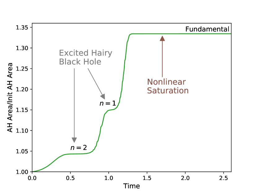
Figure 1: Apparent horizon area of a black hole as it undergoes a series of transitions through metastable excited hairy black hole states. Initial data chosen to consist primarily of $n=2$ overtone, with subleading $n=1$ overtone.

This paper is organized as follows. In section II we introduce the Einstein-Maxwell-charged scalar system and the RNAdS background solution. In section III, we review the various mode families of RNAdS and we present our linear analysis. We present our nonlinear simulations of the instabilities in section IV, with the construction of the excited hairy black holes in section IV.3. We conclude in section V. Throughout the paper, unless otherwise indicated we follow conventions of Wald (1984) and we work in four spacetime dimensions.

II Model

We consider Einstein gravity with a negative cosmological constant, coupled to Maxwell and massive charged scalar fields. The Lagrangian density is

$$\mathcal{L}=R+\frac{6}{L^{2}}-F_{ab}F^{ab}-4\left(\left|D_{a}\psi\right|^{2}-m^{2}|\psi|^{2}\right),$$ (1)

where $D_{a}\equiv\nabla_{a}-iqA_{a}$ is the gauge covariant derivative. This gives rise to the Einstein equation,

$$G_{ab}-\frac{3}{L^{2}}g_{ab}=8\pi T_{ab}^{\psi}+8\pi T_{ab}^{\mathrm{EM}},$$ (2)

with stress-energy tensors,

$$T_{ab}^{\psi}={} \frac{1}{4\pi}\left\{\frac{1}{2}\left[(D_{a}\psi)^{\ast}(D_{b}\psi)+(D_{a}\psi)(D_{b}\psi)^{\ast}\right]\right.$$

$$\left.-\frac{1}{2}g_{ab}\left(|D_{c}\psi|^{2}+m^{2}|\psi|^{2}\right)\right\},$$ (3)

$$T_{ab}^{\mathrm{EM}}={} \frac{1}{4\pi}\left(g^{cd}F_{ac}F_{bd}-\frac{1}{4}g_{ab}F_{cd}F^{cd}\right),$$ (4)

the Maxwell equation,

$$\nabla^{b}(\nabla_{b}A_{a}-\nabla_{a}A_{b})=iq\psi^{\ast}D_{a}\psi-iq\psi(D_{a}\psi)^{\ast},$$ (5)

and the Klein-Gordon equation,

$$D^{a}D_{a}\psi-m^{2}\psi=0.$$ (6)

The RNAdS black hole is a static, spherically symmetric solution with vanishing $\psi$. In Boyer-Lindquist coordinates, the metric is

$$ds^{2}=-f(r)dt^{2}+\frac{1}{f(r)}dr^{2}+r^{2}d\Omega_{2}^{2},$$ (7)

with

$$f(r)=1-\frac{2M}{r}+\frac{Q^{2}}{r^{2}}+\frac{r^{2}}{L^{2}},$$ (8)

and the Maxwell potential is

$$A_{\mu}dx^{\mu}=\left(-\frac{Q}{r}+C\right)dt.$$ (9)

We have inserted a constant $Cdt$ in $A$, which is pure gauge. We will take $C=0$ in most of this paper, so that $A(\infty)=0$. In section III.1.1, however, we will take $C=Q/r_{+}$ to set $A(r_{+})=0$, which is convenient for studying the near-horizon geometry. Under a change of gauge $C\to C+\Delta C$, the scalar field undergoes a frequency shift $\psi\to e^{iq\Delta Ct}\psi$.

We take the RNAdS solution (7)–(9) as the background for the linear analysis. Also imposing spherical symmetry, the Klein-Gordon equation (6) takes the form

$$0={} -\frac{1}{f}\partial_{t}^{2}\psi+\frac{2iqA_{0}}{f}\partial_{t}\psi+\frac{1}{r^{2}}\partial_{r}\left(r^{2}f\partial_{r}\psi\right)$$

$$-\left(m^{2}-\frac{q^{2}A_{0}^{2}}{f}\right)\psi.$$ (10)

Since $\psi$ vanishes in the background, it decouples from the other fields at linear order, and it is consistent to study $\psi$ as a test field. We analyze (II) in section III.

It is convenient to express the background quantities in terms of the inner and outer horizon radii, $r_{-}$ and $r_{+}$. The metric function becomes

$$f(r)={} \frac{(r-r_{-})(r-r_{+})}{L^{2}r^{2}}\left[r^{2}+\left(r_{-}+r_{+}\right)r\right.$$

$$\left.+\left(L^{2}+r_{-}^{2}+r_{+}^{2}+r_{-}r_{+}\right)\right],$$ (11)

from which we can read off the mass and charge of the black hole,

$$M =\frac{r_{-}+r_{+}}{2L^{2}}\left[\left(r_{+}-r_{-}\right)^{2}+L^{2}\right],$$ (12)

$$Q^{2} =\frac{r_{-}r_{+}}{L^{2}}\left(L^{2}+r_{-}^{2}+r_{+}^{2}+r_{-}r_{+}\right).$$ (13)

Thus, at extremality, $r_{+}=r_{-}$, and

$$M_{\text{ext}} =r_{+},$$ (14)

$$Q^{2}_{\text{ext}} =r_{+}^{2}\left(1+\frac{3r_{+}^{2}}{L^{2}}\right).$$ (15)

In section IV, we solve the full system of equations (2)–(6) with $m=0$ in spherical symmetry in ingoing coordinates.

III Linear perturbations

In this section we study the test scalar field (II). We begin in section III.1 by describing the mode families and instabilities that we expect to see in our numerics. In section III.2 we describe the continued fraction method for finding quasinormal frequencies numerically, and we present our results in section III.3.

III.1 Preliminaries

This section describes three families of modes that appear in the spectra we obtain in section III.3: the near-horizon mode, the AdS modes, and the zero-damped modes. These have all been derived analytically under various approximations elsewhere in the literature. We include them for completeness and for interpreting our numerical results in section III.3.

III.1.1 Near-horizon condensation instability

Four-dimensional extremal black holes with spherical horizon topology have near-horizon geometries closely related to $\mathrm{AdS}_{2}\times S^{2}$ Bardeen and Horowitz (1999); for extremal RNAdS, this correspondence becomes exact. The near-horizon instability is based on the violation of the BF bound of the near-horizon geometry by the scalar field. Holographically, the condensation corresponds to a transition to a superconducting phase below a critical temperature Gubser (2008); Hartnoll et al. (2008).

To take the near-horizon limit it is useful to set the constant $C=Q/r_{+}$ in the Maxwell field, so that $A_{a}$ vanishes on the horizon. For extremal RNAdS, we then have

$$ds^{2}_{\text{ext}} =-f_{\text{ext}}dt^{2}+\frac{1}{f_{\text{ext}}}dr^{2}+r^{2}d\Omega_{2}^{2},$$ (16)

$$A_{\text{ext}} =\frac{Q_{\text{ext}}(r-r_{+})}{rr_{+}}dt,$$ (17)

where

$$f_{\text{ext}}=\frac{(r-r_{+})^{2}}{L^{2}r^{2}}\left[r^{2}+2r_{+}r+(L^{2}+3r_{+}^{2})\right].$$ (18)

We then define a change of coordinates depending on a parameter $\lambda>0$,

$$t=\frac{\tilde{t}}{\lambda},\qquad r=r_{+}+\lambda\tilde{r}.$$ (19)

Taking the $\lambda\to 0$ limit in these coordinates, we obtain the near-horizon fields,

$$ds^{2}_{\text{NH}} = -\frac{\tilde{r}^{2}}{R^{2}}d\tilde{t}^{2}+\frac{R^{2}}{\tilde{r}^{2}}d\tilde{r}^{2}+r_{+}^{2}d\Omega_{2}^{2},$$ (20)

$$A_{\text{NH}} = \frac{Q_{\text{ext}}\tilde{r}}{r_{+}^{2}}d\tilde{t},$$ (21)

where

$$\frac{1}{R^{2}}=\frac{6}{L^{2}}+\frac{1}{r_{+}^{2}}.$$ (22)

The metric (20) is recognized as $\text{AdS}_{2}\times S^{2}$ in Poincaré coordinates, where the $\text{AdS}_{2}$ factor has radius $R$. Note that the choice of $C$ ensures that the Maxwell field remains finite in the near-horizon limit.

The scalar field acquires an effective mass in the near-horizon region. Taking the near-horizon limit of the Klein-Gordon equation (II), this is seen to be

$$m_{\text{eff}}^{2} =m^{2}-\left.\frac{q^{2}A_{0,\text{ext}}^{2}}{f_{\text{ext}}}\right|_{\lambda\to 0}$$

$$=m^{2}-q^{2}\cdot\frac{L^{2}+3r_{+}^{2}}{L^{2}+6r_{+}^{2}}.$$ (23)

In the large black hole limit, $m_{\text{eff}}^{2}\to m^{2}-q^{2}/2$. Instability can occur if $m_{\text{eff}}^{2}$ lies below the near-horizon BF bound,

$$m_{\text{NHBF}}^{2}=-\frac{1}{4R^{2}}=-\frac{1}{4}\left(\frac{6}{L^{2}}+\frac{1}{r_{+}^{2}}\right),$$ (24)

which in the large black hole limit becomes $m_{\text{NHBF}}^{2}\to-3/(2L^{2})$. It was futher shown using energy arguments that for large black holes this bound is sharp Dias et al. (2010). To be globally stable, it is necessary that the global BF bound be respected, i.e., $m^{2}\geq-9/(4L^{2})$. Thus, in the large black hole limit, the near-horizon instability is triggered if

$$-\frac{9}{4L^{2}}\leq m^{2}<-\frac{3}{2L^{2}}+\frac{q^{2}}{2},$$ (25)

which can be easily satisfied by choosing sufficiently large $q^{2}$ or negative $m^{2}$ (but not too negative). By continuity, the instability is expected to also occur for near-extreme black holes Hartnoll et al. (2008); Hollands and Ishibashi (2015).

For small black holes, it is not possible to trigger the near-horizon instability with negative $m^{2}$ since in this case the near-horizon BF bound is below the global BF bound. In addition, $q^{2}$ must be taken very large to obtain an instability, i.e.,

$$q^{2}\geq\frac{1}{4r_{+}^{2}}+m^{2}.$$ (26)

For these reasons, the near-horizon instability is said to not operate for small black holes Dias and Masachs (2017).

It should be noted that in the rest of the paper we will set the gauge constant $C\to 0$, so mode frequencies pick up an additional shift $\Delta\omega=qC=qQ/r_{+}$. In that gauge, the near-horizon unstable mode frequency for near-extreme black holes will lie near the superradiant bound frequency, $qQ/r_{+}$.

III.1.2 Superradiant instability

The superradiant instability (or “black hole bomb”) occurs when superradiant scattering is combined with a confinement mechanism, such as a mirror, a mass term, or an AdS boundary Press and Teukolsky (1972). Under superradiant scattering, an incident wave is amplified by the black hole as it extracts mass and angular momentum or charge. With the confinement mechanism, the outgoing wave cannot escape to infinity, and instead interacts repeatedly with the hole, resulting in exponential growth.

The superradiant condition is most easily derived from thermodynamic arguments Bekenstein (1973). In the charged black hole case, consider a mode solution $\psi=e^{-i\omega t}R(r)$ with real frequency $\omega$. The charge to mass ratio of the mode is

$$\frac{\delta Q}{\delta M}=\frac{q}{\omega}.$$ (27)

When the mode interacts with the black hole, it exchanges charge and mass in this ratio. The first law of black holes mechanics for charged black holes, however, is

$$\delta M=\frac{\kappa}{8\pi}\delta A_{\mathrm{H}}-\Phi_{\mathrm{H}}\delta Q,$$ (28)

where $\kappa$ is the surface gravity, $A_{\text{H}}$ is the horizon area, and $\Phi_{\mathrm{H}}$ is the electrostatic potential at the horizon. Inserting (27) into (28) relates the change in mass to the change in area of the black hole as a consequence of interacting with the mode,

$$\delta M=\frac{\kappa}{8\pi}\frac{\omega}{(\omega+\Phi_{\mathrm{H}}q)}\delta A_{\mathrm{H}}.$$ (29)

The second law of black holes mechanics states that the area of the horizon can only increase in dynamical processes, $\delta A_{\mathrm{H}}\geq 0$. Hence, waves that satisfy

$$0<\omega<-q\Phi_{\mathrm{H}}=\frac{qQ}{r_{+}}$$ (30)

will have $\delta M<0$, and will therefore extract mass and charge from the black hole.

The modes themselves are provided by the confinement mechanism. For small RNAdS, there is a set of modes that are deformations of global AdS normal modes, which have frequencies,

$$\omega_{n}^{\pm}=\pm\frac{2n+3}{L},\qquad n=0,1,2,\ldots$$ (31)

We therefore expect instability for $\omega_{n}^{+}$ with

$$2n\lesssim qQL/r_{+}-3.$$ (32)

By choosing $q$ sufficiently large, this condition is easily satisfied.

For more detailed derivations of the superradiant instability using matched asymptotic expansions we refer the reader to Uchikata and Yoshida (2011); Dias and Masachs (2017).

III.1.3 Zero-damped modes

A final class of modes that is relevant to our analysis is associated to the near-horizon region of near-extremal black holes. These long-lived “zero-damped” modes can be viewed as trapped in the extended black hole throat region.

In the asymptotically flat case, these modes were shown in Zimmerman (2017) to fall into one of two families, principal or supplementary, depending on the charge coupling and angular mode number of the scalar field. (The terminology refers to the near-horizon $SO(2,1)$ representations in which these modes lie.) Using a matched asymptotic expansion, the quasinormal frequencies of asymptotically-flat RN in spherical symmetry can be shown Zimmerman (2017) to be

$$\omega_{n}^{\text{P}}=\frac{qQ}{r_{+}}+\kappa\left[qr_{+}-i\left(\frac{1}{2}-\sqrt{\frac{1}{4}-(qr_{+})^{2}}+n\right)+\eta r_{+}\right]$$ (33)

and

$$\omega_{n}^{\text{S}}=\frac{qQ}{r_{+}}+\kappa\left[qr_{+}-i\left(\frac{1}{2}+\sqrt{\frac{1}{4}-(qr_{+})^{2}}+n\right)\right],$$ (34)

where $n=0,1,2,\ldots$ is the overtone number, $\kappa$ is the surface gravity, and $\eta$ is a small complex number. If the quantity under the square root is positive, then the supplementary family (34) applies, otherwise the principal family (33).

We see that both families consist of a $\kappa$-spaced tower of modes extending below the superradiant bound frequency. As $\kappa\to 0$ these modes converge to $qQ/r_{+}$, which becomes a branch point; this is associated to the horizon instability of Aretakis Zimmerman (2017).

Notice that the quantity under the square root in (33)–(34) becomes negative when the near-horizon instability condition (26) is satisfied, i.e., the effective mass violates the near-horizon BF bound. The frequency (33) nevertheless does not correspond to an instability in asymptotically-flat RN, as the imaginary part remains negative. For small RNAdS, we expect similar behavior, with small $(r_{+}/L)$-corrections to the quasinormal frequencies. For large RNAdS, however, we will show numerically in section III.3.2 that these modes can become unstable when the near-horizon BF bound is violated.

III.2 Continued fraction method

We now describe the continued fraction method for finding quasinormal mode solutions. We seek solutions that are ingoing at the horizon and satisfy the reflecting condition at the AdS boundary. Satisfaction of both of these conditions should yield a discrete spectrum of complex frequencies.

Let $\psi=e^{-i\omega t}R(r)$ be our mode ansatz. The Klein-Gordon equation (II) reduces to the radial equation,

$$\frac{d}{dr}\left(r^{2}f\frac{dR}{dr}\right)+\left(\frac{(\omega r^{2}-qQr)^{2}}{r^{2}f}-m^{2}r^{2}\right)R=0.$$ (35)

Asymptotically as $r\to r_{+},\infty$, this has two solutions,

$$R(r)\sim\begin{cases}(r-r_{+})^{\pm\frac{iL^{2}r_{+}\left(r_{+}\omega-qQ\right)}{\left(r_{+}-r_{-}\right)\left(L^{2}+r_{-}^{2}+3r_{+}^{2}+2r_{-}r_{+}\right)}}&\text{as }r\to r_{+},\\ r^{\frac{1}{2}\left(\pm\sqrt{4m^{2}L^{2}+9}-3\right)}&\text{as }r\to\infty.\end{cases}$$ (36)

At infinity, we require the solution to decay, so we take the solution with the minus sign as $r\to\infty$ in (36). This corresponds to a reflecting condition at the AdS boundary. To impose the ingoing condition at the horizon, we take the minus sign solution as $r\to r_{+}$.

To find a solution everywhere with the desired asymptotic behavior, we write the radial function as

$$R(r)=(r-r_{+})^{A}(r-r_{-})^{B-A}F(u),$$ (37)

where

$$A =-\frac{iL^{2}r_{+}\left(r_{+}\omega-qQ\right)}{\left(r_{+}-r_{-}\right)\left(L^{2}+r_{-}^{2}+3r_{+}^{2}+2r_{-}r_{+}\right)},$$ (38)

$$B =-\frac{1}{2}\left(\sqrt{4m^{2}L^{2}+9}+3\right),$$ (39)

and where $F(u)$ is a new unknown function with $u=(r-r_{+})/(r-r_{-})$. If $F$ is smooth on $u\in[0,1]$ then $R$ satisfies the desired asymptotic conditions.

We now expand $F$ as a power series

$$F(u)=\sum_{n=0}^{\infty}a_{n}u^{n},$$ (40)

and insert this into (35). This gives a complicated relation on the sequence $(a_{n})$, which we can simplify into a three-term recurrence relation using Gaussian reduction. We finally obtain a relation of the form

$$\alpha_{0}a_{1}+\beta_{0}a_{0} =0,$$ (41)

$$\alpha_{n}a_{n+1}+\beta_{n}a_{n}+\gamma_{n}a_{n-1} =0,\qquad n\geq 1,$$

where $\alpha_{n}$, $\beta_{n}$, and $\gamma_{n}$ all depend on $\omega$ and the system parameters. We obtained complicated closed form expressions for these coefficients, but have not included them due to space considerations.

If the series (40) converges uniformly for some value of $\omega$, then that corresponds to a quasinormal mode. To obtain such $\omega$ we use the continued fraction method of Leaver Leaver (1985) and Gautschi Gautschi (1967). (This method was recently used to compute quasinormal modes for a massless charged scalar in asymptotically flat RN Richartz and Giugno (2014).) The method relies on the fact that the power series (40) converges uniformly if the following continued fraction converges:

$$\frac{-\gamma_{1}}{\beta_{1}-\frac{\alpha_{1}\gamma_{2}}{\beta_{2}-\frac{\alpha_{2}\gamma_{3}}{\beta_{3}-...}}}.$$ (42)

Moreover, if the continued fraction (42) converges, then it is equal to $a_{1}/a_{0}$. This allows us to close the recurrence relation (41),

$$\frac{-\gamma_{1}}{\beta_{1}-\frac{\alpha_{1}\gamma_{2}}{\beta_{2}-\frac{\alpha_{2}\gamma_{3}}{\beta_{3}-...}}}=-\frac{\beta_{0}}{\alpha_{0}}.$$ (43)

Quasinormal frequencies are the values of $\omega$ that solve (43). We find these frequencies numerically by plotting the logarithm of the difference between the left and right sides of (43), and searching for negative singularities.

III.3 Results

We now present the mode spectra obtained numerically as we vary the black hole parameters, $\alpha\equiv Q/Q_{\text{ext}}$ and $r_{+}$, and the field parameters, $q$ and $m$. We fix $L=1$.

III.3.1 Small black hole

A typical quasinormal spectrum for small RNAdS is shown in figure 2. This shows two branches of modes: the vertical branch extending below the real axis is the supplementary branch (34) of zero-damped modes, and the horizontal branch is the family of AdS modes. The $n=0$ positive-frequency AdS mode lies within the band $0<\operatorname{Re}\omega<qQ/r_{+}$, and is therefore superradiantly unstable; it lies above the real axis in figure 2.

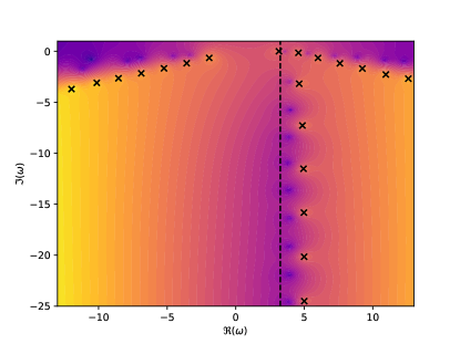
Figure 2: Continued fraction values for RNAdS with $r_{+}=0.1$, $\alpha=0.8$, $q=4$, and $m=0$. We plot the logarithm of the difference between the left hand side and right hand side of (43). Darker colors correspond to higher values. Quasinormal modes (minima in the plot) are marked by black crosses. We see that nonzero $q$ breaks the symmetry between positive and negative real part. Two branches of modes are present, a vertical branch of zero-damped modes, and a more horizontal branch AdS modes. The dashed vertical line corresponds to the superradiant bound frequency; modes satisfying $0<\operatorname{Re}\omega<qQ/r_{+}$ are unstable.

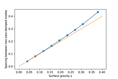
Figure 3: Spacing $\delta$ between two zero-damped modes versus surface gravity $\kappa$. Here, we take $q=0$ and $r_{+}=1$. We see that $\delta\to\kappa$ as $\kappa\to 0$.

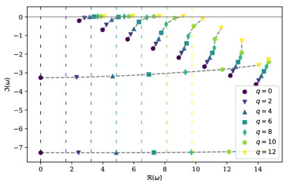
Figure 4: Quasinormal frequencies of RNAdS for $r_{+}=0.1$, $\alpha=0.8$, $m=0$, and $0\leq q\leq 12$. AdS modes become unstable when $\operatorname{Re}\omega$ drops below the superradiant bound frequency (indicated with dashed vertical lines).

For the stable AdS modes, we see that the decay rate is proportional to the distance from the superradiant strip. We have also verified that the separation between zero-damped modes is equal to $\kappa$: this is shown in figure 3 (This separation, although expected to hold only for small RNAdS, holds also for larger $r_{+}$.) In this figure, we plot the mean spacing $\delta=\langle\omega_{n+1}^{\text{S}}-\omega_{n}^{\text{S}}\rangle$ for $r_{+}=1$ and $q=0$, as a function of the surface gravity $\kappa$. We observe that $\delta\to\kappa$ as $\kappa\to 0$, in agreement with Dias and Masachs (2017).

We now study the influence of varying the field charge $q$ on the spectrum; this is shown in figure 4. As $q$ increases, so does the superradiant bound frequency, $qQ/r_{+}$. The tower of zero-damped mode frequencies remains tied to this frequency, and shifts to the right in the complex plane as well. The AdS modes also shift to the right, but more slowly than the superradiant bound frequency. One by one, these modes are overtaken by the superradiant bound frequency, and they become unstable. This is shown in figure 4.

III.3.2 Large black hole

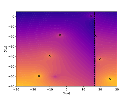
Figure 5: Continued fraction values for RNAdS with $r_{+}=5.0$ and $\alpha=0.95$, and field parameters $q=2$, $m^{2}=-1.49^{2}$. We see two diagonal branches, and one unstable mode. Not visible due to resolution is the set of zero-damped modes.

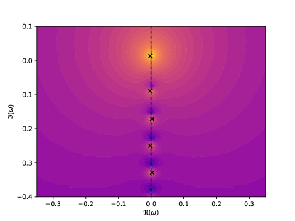
Figure 6: Quasinormal modes for $\alpha=0.995$, $r_{+}=5$, $q=0$ and $m^{2}=-1.49^{2}$. One mode in unstable here: this corresponds to the near-horizon mode.

The discussion of section III.1 indicates that for large RNAdS, we should see a near-horizon unstable mode and a tower of zero-damped modes. AdS modes, meanwhile, are known to be present only for small black holes, where they can be superradiantly unstable for large $q$, and it is not clear in general what role superradiance might play for large black holes. To disentangle the various instabilities, we use our numerical code to find and track the quasinormal modes.

A typical large RNAdS spectrum is shown in figure 5. This shows two diagonal branches of stable modes and one unstable mode. Already it is clear that the superradiant instability plays a role for large black holes, as the unstable frequency lies within the superradiant strip. In our studies, we found that, when it exists, every unstable mode lies within this strip.

To isolate the near-horizon instability, we can set $q=0$ to turn off superradiance. In the extremal case, the tachyonic instability can then be obtained with negative $m^{2}$ such that

$$-\frac{9}{4L^{2}}\leq m^{2}<-\frac{3}{2L^{2}}.$$ (44)

We choose $m^{2}=-1.49^{2}$ to bring the mass squared close to the global BF bound, and we consider a near-extremal black hole with $\alpha=0.995$. For these parameters, the quasinormal frequencies are plotted in figure 6. This shows one unstable mode, the near-horizon mode. The near-horizon mode lies close to the real axis and is thus weakly unstable. It is also apparently isolated, as we have not been able to identify a second near-horizon unstable mode when $q=0$.

Figure 6 also shows a tower of stable modes along the imaginary axis; these are the zero-damped modes. They are evenly spaced, whereas the near-horizon mode is separated by a larger distance. However, as we increased $m^{2}$ and decreased $\alpha$ to turn off the near-horizon instability, the modes re-positioned themselves into a single family. Indeed, all modes shifted downward, with the tachyonic mode dropping below the real axis and spacing itself evenly at the top of the zero-damped family. Thus, the near-horizon unstable mode is simply a member of the zero-damped family of modes. Note that the zero-damped modes should also be present in figure 5, but they are not clearly visible due to lack of resolution in this figure, and the fact that these modes are very closely spaced.

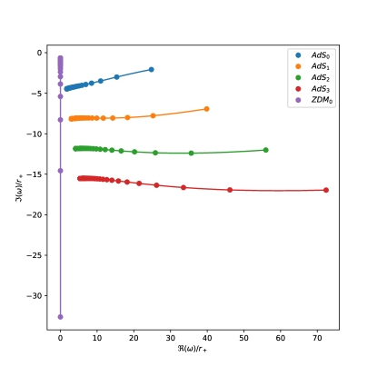
Figure 7: Tracking of the first four AdS modes ($\text{AdS}_{i}$) and the first zero-damped mode ($\text{ZDM}_{0}$) for $r_{+}$ varied between 0.1 (where the points are far apart) and $5$ (where the points are close together) by steps of $0.05$, for $\alpha=0.8$, $q=0$, and $m=0$. We observe a scaling for large black hole radius: when $r_{+}\gg L$, the modes are invariant under the transformation $r_{+}\rightarrow\lambda r_{+}$, $r_{-}\rightarrow\lambda r_{-}$, $\omega\rightarrow\lambda\omega$. This can be derived from (35). We also find that whereas for small RNAdS, the AdS modes are longest lived, for large RNAdS the zero-damped modes are longest lived.

We would now like to understand the connection between the modes of large and small RNAdS. To do so, we first track the mode frequencies as the size of the black hole is varied for $q=0$. Figure 7 shows the migration of several AdS modes and the leading zero-damped mode as $r_{+}$ is varied between $0.1$ and $5$. We observe that the diagonal branches of the large black hole in figure 5 correspond to the AdS modes for small black holes. The importance of the different mode families seems to be reversed for small and large RNAdS: for large black holes, the zero-damped modes have slowest decay, whereas the AdS modes are longest lived in the small black hole case.

Next, we increase the gauge coupling $q$ to connect the near-horizon mode to the general quasinormal spectrum of figure 5; results are presented in figure 8. We observe a very different behavior from the small black hole case of figure 4. First, the modes that become unstable are the zero-damped modes, not the AdS modes. This is not predicted by (34), which holds only for small black holes. Once unstable, zero-damped modes have a spectrum similar to the small black hole AdS-mode spectrum: the mode with smallest $\operatorname{Re}\omega$ has highest growth rate, and all unstable modes lie within the superradiant strip. Second, the AdS mode frequencies pass through a kink as they evolve; closer inspection reveals that they actually merge into the tower of zero-damped modes at large $q$.

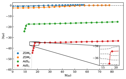
Figure 8: Quasinormal frequencies for varying $q$ for a large black hole with $r_{+}=0.1$, $\alpha=0.95$, and $m=0$. The gauge coupling $q$ varies from $0$ to $10$ by steps of $0.5$. We observe that the modes that become unstable are the zero-damped modes. The AdS mode frequencies pass through a kink in their migration: the inset shows how the second AdS mode slots itself in between two zero-damped modes.

Thus, the mode corresponding to the near-horizon instability is also the fastest growing mode in the case of a large black hole. For $q>0$, this mode lies within the superradiant strip, so violation of the near-horizon BF bound and superradiance both contribute to its instability. This is not the case for a small black hole, where the fastest-growing mode is the first AdS mode, and instability occurs even when the near-horizon BF bound is satisfied.

To summarize, for small RNAdS, unstable modes come from the AdS branch, whereas for large RNAdS, they come from the zero-damped branch. When the near-horizon BF bound is violated for large black holes, the most unstable mode also exhibits near-horizon instability. Figure 7 shows the crossover between the large and small black hole scenarios.

IV Nonlinear evolution

For our nonlinear studies, we solve the system of equations (2)–(6) numerically, with $m=0$. As in the rest of the paper, we impose spherical symmetry and reflecting boundary conditions at infinity.

In the following subsection we describe our numerical method. We then describe the evolution for generic scalar field initial data in subsection IV.2 and the excited hairy black hole in subsection IV.3.

IV.1 Method

We use the same numerical code as we used in Bosch et al. (2016). This uses ingoing Eddington-Finkelstein coordinates $(v,r)$, similar to Chesler and Yaffe (2014), but adapted to spherical symmetry. Equations are discretized with finite differences, using mixed second and fourth order radial derivative operators satisfying summation by parts (see, e.g., Calabrese et al. (2004, 2003)) and fourth order Runge-Kutta time stepping.

The spatial domain extends from an inner radius $r_{0}$, several grid points within the apparent horizon, to infinity. The singularity is thereby excised from the computational domain. To reach infinity, the domain is compactified by working with a spatial coordinate $\rho=1/r$, and defining a uniform grid on the domain $0\leq\rho\leq 1/r_{0}$.

Boundary data consist of the ADM mass $M$ and charge $Q$, and initial data are fully specified by the initial value of the scalar field, $\psi(v=0)$. The system is solved by integrating radially inward along $v=\text{constant}$ null curves to obtain the remaining field values and their time derivatives; $\psi$ is then integrated one step forward in time, and the procedure is iterated. With $\psi(v=0)=0$, this gives RNAdS with mass $M$ and charge $Q$ as the solution, but more generally some of the mass and charge is contained in the scalar field. The characteristic formulation has some residual gauge freedom, which we use to set the Maxwell potential to vanish at infinity, and to set $r$ to be the areal radius. (In Chesler and Yaffe (2014) this is used to fix the position of the horizon.) For further details, we refer the reader to Bosch et al. (2016, 2017).

The scalar field can be expanded about infinity, and with the reflecting boundary condition, this takes the form,

$$\psi(v,r)=\frac{\varphi_{3}(v)}{r^{3}}+O\left(\frac{1}{r^{4}}\right).$$ (45)

The quantity $\varphi_{3}(v)$ is an output of the simulation, and it contains information about the mode content of the solution. Other gauge-invariant output quantities are the apparent horizon area $A_{\text{H}}$ and the distribution of charge between the black hole and the scalar field. To track the superradiant bound we extract the electrostatic potential at the apparent horizon $\Phi_{\mathrm{AH}}(v)$.

IV.2 Generic evolution

We now study the evolution of large RNAdS black holes perturbed with generic scalar field configurations. We take the background solution to have $r_{+}=100$ and $Q=0.9Q_{\text{ext}}$, fixing $L=1$ throughout. Strictly speaking, we only have control over the ADM quantities (which we impose as boundary data) but we take the initial scalar field to have very small amplitude, so to a good approximation these directly determine the background black hole parameters.

We take the scalar field initial data to be compactly supported outside the black hole, with profile $\psi(v=0)=(r^{-1}-r_{1}^{-1})^{3}\ (r^{-1}-r_{2}^{-1})^{3}\ (\kappa_{1}+\kappa_{2}\sin(10r^{-1}))/r^{2}$ for $r_{+}<r_{1}\leq r\leq r_{2}<\infty$, and zero otherwise. The observed dynamics are qualitatively similar to the small black hole superradiant instability Bosch et al. (2016): when the black hole is unstable, charge and mass are extracted by the scalar field until a stationary hairy black hole final state is reached. The final state is, moreover, independent of the initial scalar field profile.

We experimented with varying the gauge coupling $q$; figure 9 shows the area of the apparent horizon as a function of time for several different values. For larger $q$, the final area is larger, and the growth in area happens over a much shorter time scale. Indeed, for the smallest value, $q=4$, the area grows by just a few percent, whereas for larger values, $q>200$, it more than doubles. Figures 10 and 11 show the extraction of charge and the final radial profile of $\psi$, respectively. Indeed, the field has support closer to the black hole for the smaller values of $q$, consistent with the near-horizon instability Murata et al. (2010). For larger values of $q$, more charge is extracted, and the field has support further from the black hole. For very large $q$, nearly all the charge is extracted, and the final state is nearly Schwarzschild, with a scalar condensate far away. In all cases, the field profile has a single peak, so the condensate is in its ground state.

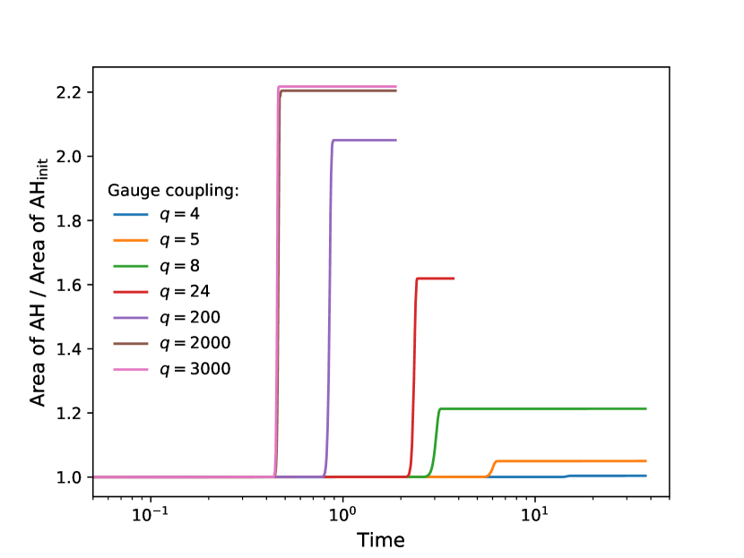
Figure 9: Normalized area of the apparent horizon as a function of time, for initial black hole with $r_{+}=100$ and $Q=0.9Q_{\text{ext}}$. Different colors correspond to different gauge coupling $q$.

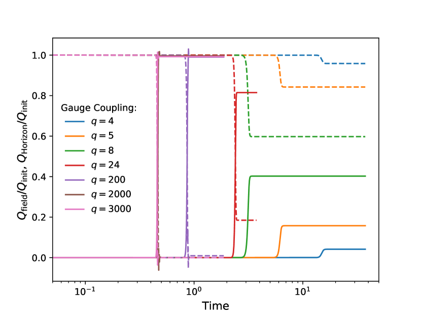
Figure 10: Normalized charge contained in the black hole and in the scalar field as a function of time, for initial black hole with $r_{+}=100$ and $Q=0.9Q_{\text{ext}}$. Solid lines denote scalar field charge, and the dashed lines denote black hole charge.

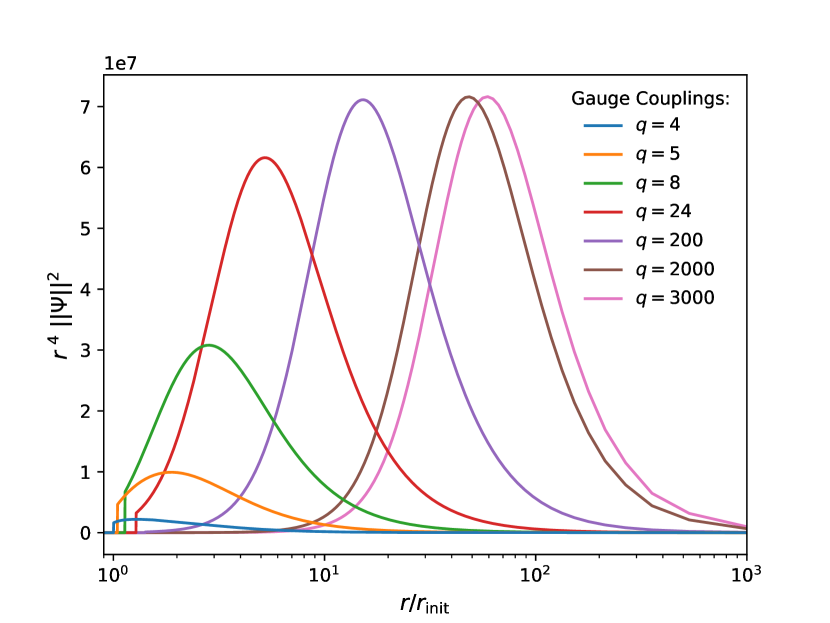
Figure 11: End state radial profile of the scalar field, for initial black hole with $r_{+}=100$ and $Q=0.9Q_{\mathrm{ext}}$. For smaller gauge coupling $q$ the field has support closer to the horizon, whereas for larger $q$ the support is away from the black hole.

It is useful to examine also the dynamics of the boundary values of the scalar field, $\varphi_{3}(v)$. We present a time-frequency analysis in figure 12 for the $q=24$ case. The peaks correspond to quasinormal modes, and we see that at early times, there are nine unstable modes, with the fastest growth rate for the lowest frequency. As mass and charge are extracted, however, the superradiant bound frequency decreases, and the higher frequency modes begin to decay (cf. figure 4). Eventually only the fundamental $n=0$ mode remains. The final state is reached when the superradiant bound frequency matches the $n=0$ mode frequency, so that this mode becomes marginally stable. Notice the shift in the $n=0$ mode frequency over a very short time period just before saturation; this occurs because the background solution evolves very rapidly just before saturation, as seen in figures 9 and 10.

$n$	$\omega$
0	$1780.01+17.29i$
1	$2277.33+16.59i$
2	$2655.28+14.29i$
3	$2952.42+11.97i$
4	$3188.37+9.83i$
5	$3374.87+7.89i$
6	$3519.76+6.15i$
7	$3628.68+4.55i$
8	$3705.19+3.00i$

Table 1: Quasinormal frequencies for $r_{+}=100$, $Q=0.9Q_{\mathrm{ext}}$, and $q=24$. The superradiant bound frequency is $-q\Phi_{\mathrm{H}}=3741.29$. The growth rate $\operatorname{Im}\omega$ decreases as the overtone number $n$ grows.

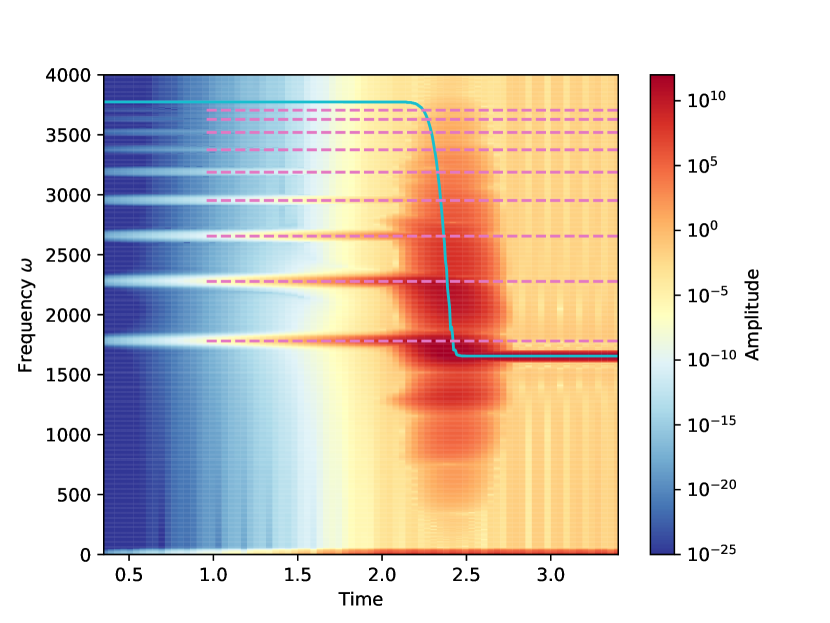
Figure 12: Spectrogram of $\operatorname{Re}\varphi_{3}(v)$ for evolution starting from $r_{+}=100$, $Q=0.9Q_{\text{ext}}$, and $q=24$. Initially there are nine unstable modes; in the end, the final state is in the fundamental mode. Dashed lines correspond to the quasinormal frequencies of table 1, solid to the superradiant bound frequency, $-q\Phi_{\mathrm{AH}}(v)$.

IV.3 Excited hairy black hole

IV.3.1 Initial data

We have seen in the previous subsection that the final state for generic initial data always corresponds to the fundamental superradiant mode, even in the case where multiple unstable modes are present. In all cases examined, the growth rate of individual modes decreases with increasing overtone number $n$; the fundamental mode grows fastest, as seen in table 1. For generic initial data—with many modes initially excited—the evolution, after possibly complicated dynamics, always comes to be dominated by the fundamental mode.

Nevertheless, for special initial data—with overtone modes excited to higher amplitude—the evolution could be dominated (at least for some time) by $n>0$ modes. If this time is longer than the saturation time for the overtone instability, then the system will reach the excited hairy black hole equilibrium.

To obtain suitable initial data, we require precise overtone mode functions. To obtain these, we first select parameters $r_{+}$, $Q$ and $q$ such that the background RNAdS solution has multiple unstable modes, and then we use the method of section III.2 to calculate precise quasinormal frequencies. We then insert the mode ansatz $\psi(v,r)=e^{-i\omega v}R(r)$ in ingoing Eddington-Finkelstein coordinates into (6) to obtain the radial equation for frequency $\omega$. For each desired overtone, we integrate this ordinary differential equation numerically, with reflecting boundary conditions at the AdS boundary. The mode can then be taken as initial data at advanced time $v=0$.

We consider two types of special initial data. The first consists of a single overtone mode $\psi_{n}$, which, if pure enough, we expect to evolve into an excited hairy black hole. The second type of initial data is a mixture of two modes, i.e.,

$$\psi_{\text{mix}}=a_{\text{mix}}\psi_{2}+(1-a_{\text{mix}})\psi_{1},$$ (46)

with, e.g., $a_{\text{mix}}=0.999$, and the amplitudes normalized using the infinity norm. With these data, we hope to achieve a cascade, where initially a $n=2$ excited black hole forms, which then decays to $n=1$, and then $n=0$. Some initial data profiles are shown in figure 13.

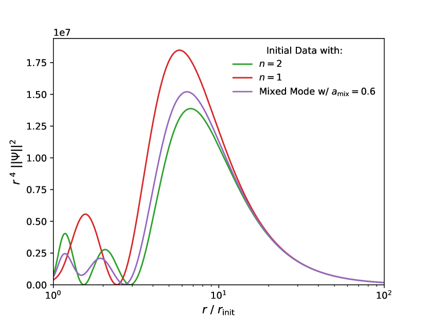
Figure 13: Radial profiles of initial data for initial values $r_{+}=100$, $Q=0.9Q_{\mathrm{ext}}$, and $q=11$. Two curves correspond to single-mode data, and the third to mixed-mode data.

IV.3.2 Results

As in the generic evolution, we fix $r_{+}=100$, $Q=0.9Q_{\text{ext}}$, and $L=1$. We then consider two cases for the scalar field charge, $q=8,11$. The significance of these latter two choices is that for $q=8$, the background RNAdS solution has two unstable modes, whereas for $q=11$, there are three unstable modes.

q=8: In this case, modes $n=0,1$ are unstable, with initial quasinormal frequencies $\omega_{0}=978.70+7.34i$ and $\omega_{1}=1168.69+4.79i$. To obtain the $n=1$ excited hairy black hole, we take initial data to consist of $\psi_{1}$. We find that under evolution, the mode grows exponentially and extracts charge and mass from the black hole, similar to the generic evolution. This causes the superradiant bound frequency, $-q\Phi_{\text{H}}$, to drop until it matches $\operatorname{Re}\omega_{1}$. (The mode frequency $\operatorname{Re}\omega_{1}$ evolves due to the changing background spacetime, but this is negligible compared to the change in superradiant bound frequency.) At this point, superradiance stops, and the system settles into the excited hairy black hole state. The black hole is static, with the scalar field oscillating harmonically.

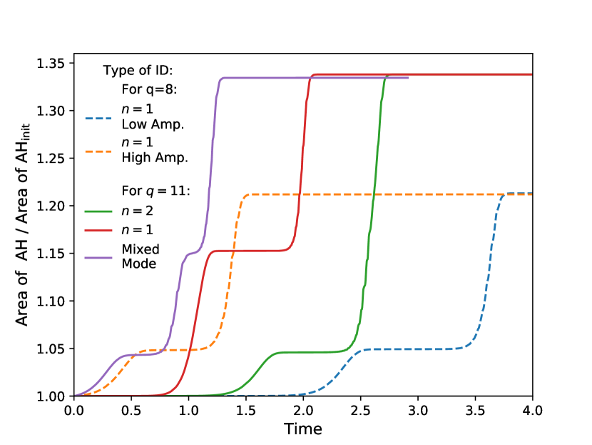
Figure 14: Normalized area of the apparent horizon for initial $r_{+}=100$ and $Q=0.9Q_{\text{ext}}$. Dashed curves correspond to $q=8$, solid to $q=11$. Excited hairy black hole solutions occur at the temporary plateaus.

The area of the apparent horizon is shown in figure 14 (either one of the dashed curves). The excited hairy black hole is seen as a plateau, where the area stops growing because the scalar field is no longer extracting mass and charge. To this point, the description parallels that of section IV.2. However, after some time, the area begins to grow again; this is because the $n=0$ mode was present and growing the entire time. Indeed, since $\operatorname{Re}\omega_{0}<\operatorname{Re}\omega_{1}$, the fundamental mode remains superradiantly unstable even after the overtone saturates. When the amplitude of the $n=0$ mode becomes large, it disrupts the static black hole and causes its area to grow significantly. Once $-q\Phi_{\text{H}}$ drops below $\operatorname{Re}\omega_{1}$, the overtone mode falls back into the black hole, and once it reaches $\operatorname{Re}\omega_{0}$, superradiance stops completely. At this point, the black hole is in its final state, described by the $n=0$ ground state mode.

It is impossible to avoid triggering the $n=0$ mode. At the initial time, the data for $\psi_{1}$ will always have numerical error, which will have some overlap with $\psi_{0}$. Moreover, during evolution, $\psi_{0}$ will be excited nonlinearly. To determine the origin of the observed $n=0$ mode, we varied the initial perturbation amplitude, and read off the times $t_{1}$ and $t_{0}$ at which the $n=1$ mode saturates and the $n=0$ mode overtakes the dynamics, respectively. Using the growth rates from the linear analysis we know that

$$\log\left(\frac{A_{1}}{A_{0}}\right)=t_{0}\operatorname{Im}{\omega_{0}}-t_{1}\operatorname{Im}{\omega_{1}}\,,$$ (47)

where $A_{1}$ and $A_{0}$ are the initial amplitudes respectively. We used this formula to calculate the amplitude $A_{0}$, given $A_{1}$ and the measured $t_{0}$, $t_{1}$.

For sufficiently small $A_{1}$, the calculated $A_{0}$ has only a mild dependence on $A_{1}$ indicating the zero mode is sourced primarily by truncation. (This was confirmed by noting the onset of this behavior depends on the resolution, with finer resolutions showing such behavior at smaller values of $A_{1}$.) However, for $A_{1}\gtrsim 5\times 10^{-3}$, we found that

$$A_{0}\sim A_{1}^{\phantom{1}2.75\pm 0.07},$$ (48)

This value is consistent with the seed arising from the self-gravitating contribution of the scalar field ($A_{0}\propto A_{1}^{\phantom{1}3}$).

Evolutions with “low” and “high” initial perturbation amplitudes are depicted in figure 14. Notice that although the saturation times differ between the two cases, the areas of the hairy black holes are largely independent of the amplitude of the initial data, as long as the amplitude is low.

q=11: For $q=11$, modes $n=0,1,2$ are unstable, with frequencies $\omega_{0}=1174.13+9.94i$, $\omega_{1}=1448.56+8.06i$, and $\omega_{2}=1615.34+5.20i$. We therefore consider three types of initial data, data with modes $n=1$ and $n=2$ individually excited, and the mixed-mode initial data (46). Simulation results for the apparent horizon area are shown as solid curves in figure 14.

The behavior for single-mode initial data is qualitatively similar to $q=8$. We find, however, that the area of the $n=1$ excited hairy black hole is larger than the $n=2$ black hole, consistent with the discussion above and $\operatorname{Re}\omega_{1}<\operatorname{Re}\omega_{2}$. The final black hole is the same in both single-mode cases. In figure 15 we plot the electric charge of the black hole and the scalar field. This shows that at the end of the excited hairy black hole life, significant amounts of charge are deposited back into the hole. This corresponds to the rapid decay of overtone hair as the superradiant bound frequency drops below the overtone frequency (cf. figure 5, where quasinormal mode decay time scales are much shorter than growth time scales).

For mixed-mode initial data, we take mixing ratio $a_{\mathrm{mix}}=0.999$, i.e., the data are $99.9\%$ $n=2$ and $0.1\%$ $n=1$. This allows the $n=2$ mode to dominate the dynamics for early times. The length of time the $n=2$ will dominate can be estimated, using a similar calculation to (47), to be $\Delta t=(\log(a_{\mathrm{mix}}/(1-a_{\mathrm{mix}}))+t_{\mathrm{s}}(\operatorname{Im}{\omega_{2}}-\operatorname{Im}{\omega_{1}}))/\operatorname{Im}{\omega_{1}}\sim 0.66$, where $t_{\mathrm{s}}$ is the time at which the $n=2$ mode saturates. Indeed, we observe (purple solid curve in figures 14 and 15) that the system cascades through two transient excited hairy black hole states, first $n=2$, then $n=1$, before settling in the ground state. The hairy black hole states match those seen in the single-mode evolutions.

We present a spectrogram for the mixed-mode evolution in figure 16. This shows a clear progression through the three unstable modes. Notice again that the final $n=0$ oscillation frequency is slightly lower than the frequency of the initial $n=0$ quasinormal mode. This shift arises because the final black hole is different from the initial one, and the superradiant bound frequency has shifted.

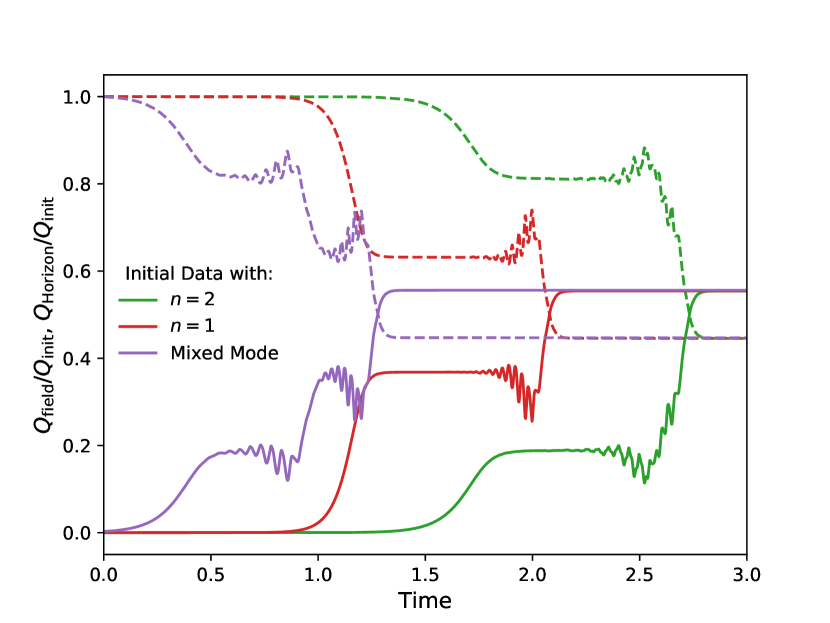
Figure 15: Charge transfer as a function of time for initial data with $r_{+}=100$, $Q=0.9Q_{\text{ext}}$, and $q=11$. Solid curves are the (normalized) charge of the scalar field, dashed curves the charge of the black hole.

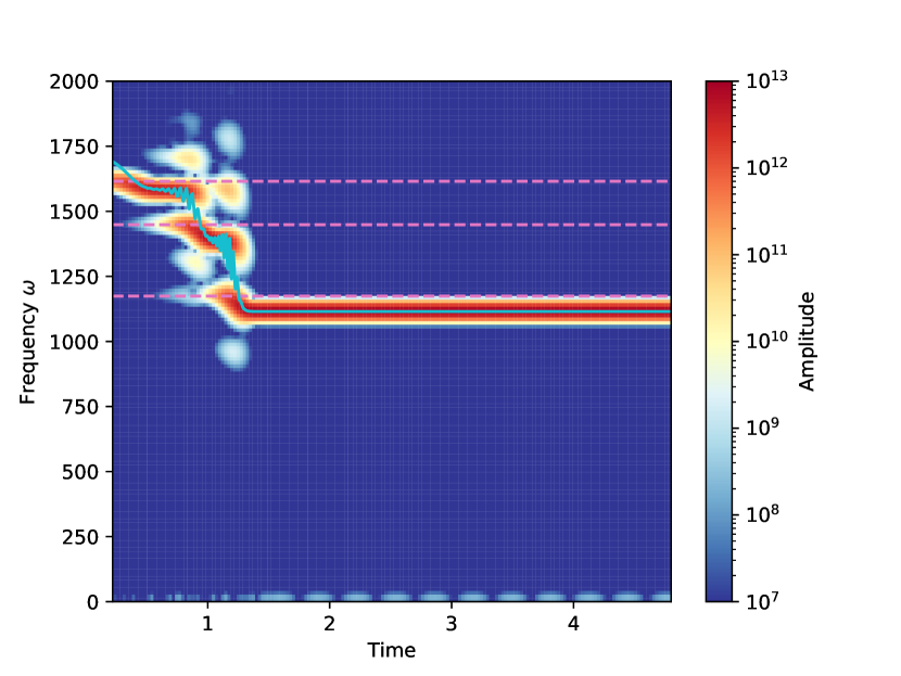
Figure 16: Spectrogram of $\varphi_{3}(v)$ for mixed mode initial data, with $r_{+}=100$, $Q=0.9Q_{\text{ext}}$, $q=11$, and $a_{\mathrm{Mix}}=0.999$. This shows a cascade through hairy black holes with $n=2\rightarrow 1\rightarrow 0$. Dashed lines indicate values of the initial mode frequencies (calculated using the linear analysis), solid corresponds to the superradiant bound $-q\Phi_{\mathrm{AH}}(v)$.

V Conclusions

In this work we computed the $l=0$ charged scalar quasinormal mode spectrum for RNAdS, and in cases of unstable modes, we numerically simulated the full nonlinear development.

The quasinormal mode analysis used the continued fraction method, which enabled us to study regions of parameter space that were not previously examined due to a lack of small parameter needed for analytic studies. We showed in particular that for large black holes, the zero-damped mode family can become superradiantly unstable, and exhibits behavior similar to the small black hole AdS mode family. Furthermore, the leading unstable mode is identified with the near-horizon condensation instability.

At the nonlinear level, we studied the evolution of these large-RNAdS unstable modes. We showed that the generic end point is a static black hole with a (harmonically-oscillating) scalar condensate, similar to earlier results for small Bosch et al. (2016) and planar Murata et al. (2010) RNAdS. We also showed that for black holes with multiple unstable modes, special initial data can be chosen that evolve to a transient excited hairy black hole solution before decaying to the generic end state.

It is tempting to draw an analogy between classical hairy black hole energy levels and quantum energy levels of atoms. In this picture (in AdS) the scalar field can only exchange energy (and charge and angular momentum) with the black hole, so the horizon plays the role of the atomic environment. In the black hole case, however, level transitions can only occur in the direction of decreasing overtone number. Transitions in the reverse direction are forbidden by the area theorem.

The reason that the final hairy black hole is always in the $n=0$ configuration is because out of all quasinormal modes, the $n=0$ mode has lowest $\operatorname{Re}\omega>0$. The superradiance condition is $0<\operatorname{Re}\omega<-q\Phi_{\text{H}}$, and as mass and charge extraction cause the upper bound to decrease, the $n=0$ mode is the last to remain unstable. We were nevertheless able to obtain the transient excited hairy black holes because the instability growth rates of the overtones are comparable and we were free to choose special overtone initial data.

Had the growth rate of overtone modes been higher than the fundamental mode, the situation would be somewhat different. Although the final configuration would be unchanged (because of the ordering of the real parts of the frequencies), the excited hairy black hole states would occur transiently for generic initial data. This reverse ordering of overtone growth rates occurs for superradiantly-unstable angular harmonics of Proca fields in Kerr Siemonsen and East (2019), which is relevant to searches for ultralight dark matter Arvanitaki et al. (2015). It would be interesting to study any observational consequences of transient overtone equilibria in this context.

Another context where the interplay between instability criteria and growth rates leads to transient states in generic evolutions is the superradiant instability of Kerr-AdS. These states, however, involve different angular harmonics rather than radial overtones. Indeed recent simulations Chesler and Lowe (2019) of the Kerr-AdS superradiant instability show an evolution dominated by a series of epochs consisting of black resonators Dias et al. (2015), which are themselves unstable Green et al. (2016).

Instability of RNAdS and subsequent hairy black hole formation has been proposed as a holographic dual to a superconducting phase transition Hartnoll et al. (2008); Horowitz et al. (2011). It is intriguing to seek also a holographic interpretation of the transient hairy black hole equilibria that we uncovered.

More generally, our work underscores the importance of overtone modes and nonlinear effects in black hole perturbations. For perturbed black holes arising from a binary merger, recent works Giesler et al. (2019); Isi et al. (2019); Ota and Chirenti (2019) have argued that the post-merger gravitational-wave signal can be well-described by a combination of overtone modes evolving linearly in a Kerr background. Other works, however, have argued for additional nonlinear mode excitation Zlochower et al. (2003); East et al. (2014), sometimes through parametric instabilities Yang et al. (2015a, b). For weakly perturbed black holes, we measured a natural scaling (48) that describes nonlinear mode excitation in RNAdS. Further work and numerical simulations will be needed to build intuition and understand the validity of linear analyses in strongly perturbed regimes.

Appendix A Code validation

We have confirmed the validity of both codes used extensively in this work through self-convergence tests as well as comparison with available results in suitable regimes. With regards to self-convergence tests, we have verified that as the number of terms employed in the continued fraction method is increased, our results asymptote to consistent results and, that typically this takes place when $N\gtrapprox 3000$ (see figure 17). Convergence of the non-linear code has been recently demonstrated in Bosch et al. (2016). As mentioned, we also compare with specific results; in particular: our QNM frequencies obtained in our linear analysis agree with those obtained in Horowitz and Hubeny (2000) in the Schwarzschild-AdS limit ($Q=0$,$q=0$) to better than $1.2\%$ for the real part of $\omega$ and better than $0.5\%$ for the imaginary part of $\omega$. In the charged, small black hole case, our results agree with those presented in Uchikata and Yoshida (2011) to better than $0.1\%$. An example of these comparisons is given in Tables 2,3. In the large black hole, small charge regime, our results agree with those in Berti and Kokkotas (2003). to better than $7.5\%$ and $4\%$ for the real and imaginary parts of $\omega$ respectively. We have also confirmed solutions obtained with our full non-linear simulations illustrate initial growth rates –in the unstable regime– and black hole QNMs consistent with the expected results from our linear studies.

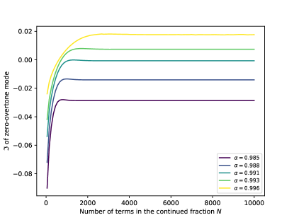
Figure 17: Imaginary part of the NH mode as a function of the number of terms used in the continued fraction $N$, for different values of the extremality parameter $a$. We can observe that convergence is more difficult when $a$ gets closer to 1, as the equations used break down.

	Values of Horowitz and Hubeny (2000)		Our values
$r_{+}$	$\operatorname{Re}(\omega)$	$\operatorname{Im}(\omega)$	$\operatorname{Re}(\omega)$	$\operatorname{Im}(\omega)$
0.4	$2.3629$	$-1.0064$	$2.3629$	$-1.0065$
0.6	$2.4316$	$-1.5797$	$2.4316$	$-1.5797$
0.8	$2.5878$	$-2.1304$	$2.5878$	$-2.1304$
1	$2.7982$	$-2.6712$	$2.7982$	$-2.6712$
5	$9.4711$	$-13.3255$	$9.4711$	$-13.3255$
10	$18.6070$	$-26.6418$	$18.6070$	$-26.6418$
50	$92.4937$	$-133.1933$	$92.4937$	$-133.1933$
100	$184.9534$	$-266.3856$	$184.9534$	$-266.3856$

Table 2: QNMs found by the linear analysis for a Schwarzschild black hole ($a=0$, $q=0$) and comparison with the results of Horowitz and Hubeny (2000) (Table 1). We can see our values agree completely with the previous results.

		Values of Uchikata and Yoshida (2011)		Our values
$q$	$a$	$\operatorname{Re}(\omega)$	$\operatorname{Im}(\omega)$	$\operatorname{Re}(\omega)$	$\operatorname{Im}(\omega)$
0	0	$2.6928$	$-1.0095\text{\times}{10}^{-1}$	$2.6928$	$-1.0096\text{\times}{10}^{-1}$
	0.2	$2.6801$	$-1.0434\text{\times}{10}^{-1}$	$2.6801$	$-1.0434\text{\times}{10}^{-1}$
	0.4	$2.6410$	$-1.1625\text{\times}{10}^{-1}$	$2.6411$	$-1.1626\text{\times}{10}^{-1}$
	0.6	$2.5723$	$-1.4417\text{\times}{10}^{-1}$	$2.5723$	$-1.4417\text{\times}{10}^{-1}$
	0.8	$2.4787$	$-2.0756\text{\times}{10}^{-1}$	$2.4788$	$-2.0757\text{\times}{10}^{-1}$
	0.9	$2.4332$	$-2.5493\text{\times}{10}^{-1}$	$2.4332$	$-2.5493\text{\times}{10}^{-1}$
2	0.2	$2.7614$	$-8.1233\text{\times}{10}^{-2}$	$2.7615$	$-8.1233\text{\times}{10}^{-2}$
	0.4	$2.8058$	$-6.7765\text{\times}{10}^{-2}$	$2.8059$	$-6.7765\text{\times}{10}^{-2}$
	0.6	$2.8256$	$-5.8950\text{\times}{10}^{-2}$	$2.8257$	$-5.8950\text{\times}{10}^{-2}$
	0.8	$2.8161$	$-5.6894\text{\times}{10}^{-2}$	$2.8161$	$-5.6894\text{\times}{10}^{-2}$
	0.9	$2.7977$	$-6.3772\text{\times}{10}^{-2}$	$2.7978$	$-6.3773\text{\times}{10}^{-2}$
4	0.2	$2.8414$	$-6.1698\text{\times}{10}^{-2}$	$2.8415$	$-6.1698\text{\times}{10}^{-2}$
	0.4	$2.9650$	$-3.4408\text{\times}{10}^{-2}$	$2.9650$	$-3.4408\text{\times}{10}^{-2}$
	0.6	$3.0672$	$-1.3945\text{\times}{10}^{-2}$	$3.0672$	$-1.3946\text{\times}{10}^{-2}$
	0.8	$3.1515$	$1.7314\text{\times}{10}^{-3}$	$3.1515$	$1.7314\text{\times}{10}^{-3}$
	0.9	$3.1878$	$6.5742\text{\times}{10}^{-3}$	$3.1879$	$6.5744\text{\times}{10}^{-3}$

Table 3: QNMs found by the linear analysis for a small black hole ($r_{+}=0.1$) and comparison with the results of Uchikata and Yoshida (2011) (Table 2). We can see our values agree completely with the previous results.

References

- Choptuik (1993) Matthew W. Choptuik, “Universality and scaling in gravitational collapse of a massless scalar field,” Phys. Rev. Lett. 70, 9–12 (1993).
- Gundlach (1999) Carsten Gundlach, “Critical phenomena in gravitational collapse,” Living Rev. Rel. 2, 4 (1999), arXiv:gr-qc/0001046 [gr-qc] .
- Bizon and Rostworowski (2011) Piotr Bizon and Andrzej Rostworowski, “On weakly turbulent instability of anti-de Sitter space,” Phys. Rev. Lett. 107, 031102 (2011), arXiv:1104.3702 [gr-qc] .
- Carrasco et al. (2012) Federico Carrasco, Luis Lehner, Robert C. Myers, Oscar Reula, and Ajay Singh, “Turbulent flows for relativistic conformal fluids in 2+1 dimensions,” Phys. Rev. D86, 126006 (2012), arXiv:1210.6702 [hep-th] .
- Yang et al. (2015a) Huan Yang, Aaron Zimmerman, and Luis Lehner, “Turbulent Black Holes,” Phys. Rev. Lett. 114, 081101 (2015a), arXiv:1402.4859 [gr-qc] .
- Adams et al. (2014) Allan Adams, Paul M. Chesler, and Hong Liu, “Holographic turbulence,” Phys. Rev. Lett. 112, 151602 (2014), arXiv:1307.7267 [hep-th] .
- Press and Teukolsky (1972) William H. Press and Saul A. Teukolsky, “Floating Orbits, Superradiant Scattering and the Black-hole Bomb,” Nature 238, 211–212 (1972).
- Arvanitaki and Dubovsky (2011) Asimina Arvanitaki and Sergei Dubovsky, “Exploring the String Axiverse with Precision Black Hole Physics,” Phys. Rev. D83, 044026 (2011), arXiv:1004.3558 [hep-th] .
- East (2017) William E. East, “Superradiant instability of massive vector fields around spinning black holes in the relativistic regime,” Phys. Rev. D96, 024004 (2017), arXiv:1705.01544 [gr-qc] .
- Hartnoll et al. (2008) Sean A. Hartnoll, Christopher P. Herzog, and Gary T. Horowitz, “Holographic Superconductors,” JHEP 12, 015 (2008), arXiv:0810.1563 [hep-th] .
- Gubser (2008) Steven S. Gubser, “Breaking an Abelian gauge symmetry near a black hole horizon,” Phys. Rev. D78, 065034 (2008), arXiv:0801.2977 [hep-th] .
- Bekenstein (1995) Jacob D. Bekenstein, “Novel “no-scalar-hair” theorem for black holes,” Phys. Rev. D 51, R6608–R6611 (1995).
- Herdeiro and Radu (2015) Carlos A. R. Herdeiro and Eugen Radu, “Asymptotically flat black holes with scalar hair: a review,” Proceedings, 7th Black Holes Workshop 2014: Aveiro, Portugal, December 18-19, 2014, Int. J. Mod. Phys. D24, 1542014 (2015), arXiv:1504.08209 [gr-qc] .
- Hollands and Wald (2013) Stefan Hollands and Robert M. Wald, “Stability of Black Holes and Black Branes,” Commun. Math. Phys. 321, 629–680 (2013), arXiv:1201.0463 [gr-qc] .
- Gregory and Laflamme (1993) R. Gregory and R. Laflamme, “Black strings and p-branes are unstable,” Phys. Rev. Lett. 70, 2837–2840 (1993), arXiv:hep-th/9301052 [hep-th] .
- Lehner and Pretorius (2010) Luis Lehner and Frans Pretorius, “Black Strings, Low Viscosity Fluids, and Violation of Cosmic Censorship,” Phys. Rev. Lett. 105, 101102 (2010), arXiv:1006.5960 [hep-th] .
- Murata et al. (2010) Keiju Murata, Shunichiro Kinoshita, and Norihiro Tanahashi, “Non-equilibrium Condensation Process in a Holographic Superconductor,” JHEP 07, 050 (2010), arXiv:1005.0633 [hep-th] .
- Bosch et al. (2016) Pablo Bosch, Stephen R. Green, and Luis Lehner, “Nonlinear Evolution and Final Fate of Charged Anti–de Sitter Black Hole Superradiant Instability,” Phys. Rev. Lett. 116, 141102 (2016), arXiv:1601.01384 [gr-qc] .
- Dias and Masachs (2017) Óscar J. C. Dias and Ramon Masachs, “Hairy black holes and the endpoint of AdS4 charged superradiance,” JHEP 02, 128 (2017), arXiv:1610.03496 [hep-th] .
- Leaver (1985) E. W. Leaver, “An analytic representation for the quasi-normal modes of kerr black holes,” Proceedings of the Royal Society A: Mathematical, Physical and Engineering Sciences 402, 285–298 (1985).
- Uchikata and Yoshida (2011) Nami Uchikata and Shijun Yoshida, “Quasinormal modes of a massless charged scalar field on a small Reissner-Nordstrom-anti-de Sitter black hole,” Phys. Rev. D83, 064020 (2011), arXiv:1109.6737 [gr-qc] .
- Bardeen and Horowitz (1999) James M. Bardeen and Gary T. Horowitz, “The Extreme Kerr throat geometry: A Vacuum analog of ,” Phys. Rev. D60, 104030 (1999), arXiv:hep-th/9905099 [hep-th] .
- Breitenlohner and Freedman (1982) Peter Breitenlohner and Daniel Z. Freedman, “Positive Energy in anti-De Sitter Backgrounds and Gauged Extended Supergravity,” Phys. Lett. 115B, 197–201 (1982).
- Abdalla et al. (2010) E. Abdalla, C. E. Pellicer, Jeferson de Oliveira, and A. B. Pavan, “Phase transitions and regions of stability in reissner-nordström holographic superconductors,” Phys. Rev. D 82, 124033 (2010).
- Maeda et al. (2010) Kengo Maeda, Shunsuke Fujii, and Jun-ichirou Koga, “Final fate of instability of reissner-nordström-anti-de sitter black holes by charged complex scalar fields,” Phys. Rev. D 81, 124020 (2010).
- Hollands and Ishibashi (2015) Stefan Hollands and Akihiro Ishibashi, “Instabilities of extremal rotating black holes in higher dimensions,” Commun. Math. Phys. 339, 949–1002 (2015), arXiv:1408.0801 [hep-th] .
- Zimmerman (2017) Peter Zimmerman, “Horizon instability of extremal Reissner-Nordström black holes to charged perturbations,” Phys. Rev. D95, 124032 (2017), arXiv:1612.03172 [gr-qc] .
- Aretakis (2015) Stefanos Aretakis, “Horizon Instability of Extremal Black Holes,” Adv. Theor. Math. Phys. 19, 507–530 (2015), arXiv:1206.6598 [gr-qc] .
- Wald (1984) Robert M. Wald, General Relativity (University of Chicago Press, Chicago, IL, 1984).
- Dias et al. (2010) Oscar J. C. Dias, Pau Figueras, Ricardo Monteiro, Harvey S. Reall, and Jorge E. Santos, “An instability of higher-dimensional rotating black holes,” JHEP 05, 076 (2010), arXiv:1001.4527 [hep-th] .
- Bekenstein (1973) Jacob D. Bekenstein, “Extraction of energy and charge from a black hole,” Phys. Rev. D 7, 949–953 (1973).
- Gautschi (1967) Walter Gautschi, “Computational aspects of three-term recurrence relations,” SIAM Review 9, 24–82 (1967).
- Richartz and Giugno (2014) Maurício Richartz and Davi Giugno, “Quasinormal modes of charged fields around a reissner-nordström black hole,” Physical Review D 90 (2014), 10.1103/physrevd.90.124011.
- Chesler and Yaffe (2014) Paul M. Chesler and Laurence G. Yaffe, “Numerical solution of gravitational dynamics in asymptotically anti-de Sitter spacetimes,” JHEP 07, 086 (2014), arXiv:1309.1439 [hep-th] .
- Calabrese et al. (2004) Gioel Calabrese, Luis Lehner, Oscar Reula, Olivier Sarbach, and Manuel Tiglio, “Summation by parts and dissipation for domains with excised regions,” Class. Quant. Grav. 21, 5735–5758 (2004), arXiv:gr-qc/0308007 [gr-qc] .
- Calabrese et al. (2003) Gioel Calabrese, Luis Lehner, David Neilsen, Jorge Pullin, Oscar Reula, Olivier Sarbach, and Manuel Tiglio, “Novel finite differencing techniques for numerical relativity: Application to black hole excision,” Class. Quant. Grav. 20, L245–L252 (2003), arXiv:gr-qc/0302072 [gr-qc] .
- Bosch et al. (2017) Pablo Bosch, Alex Buchel, and Luis Lehner, “Unstable horizons and singularity development in holography,” JHEP 07, 135 (2017), arXiv:1704.05454 [hep-th] .
- Siemonsen and East (2019) Nils Siemonsen and William E. East, “Gravitational wave signatures of ultralight vector bosons from black hole superradiance,” (2019), arXiv:1910.09476 [gr-qc] .
- Arvanitaki et al. (2015) Asimina Arvanitaki, Masha Baryakhtar, and Xinlu Huang, “Discovering the QCD Axion with Black Holes and Gravitational Waves,” Phys. Rev. D91, 084011 (2015), arXiv:1411.2263 [hep-ph] .
- Chesler and Lowe (2019) Paul M. Chesler and David A. Lowe, “Nonlinear Evolution of the AdS4 Superradiant Instability,” Phys. Rev. Lett. 122, 181101 (2019), arXiv:1801.09711 [gr-qc] .
- Dias et al. (2015) Óscar J. C. Dias, Jorge E. Santos, and Benson Way, “Black holes with a single Killing vector field: black resonators,” JHEP 12, 171 (2015), arXiv:1505.04793 [hep-th] .
- Green et al. (2016) Stephen R. Green, Stefan Hollands, Akihiro Ishibashi, and Robert M. Wald, “Superradiant instabilities of asymptotically anti-de Sitter black holes,” Class. Quant. Grav. 33, 125022 (2016), arXiv:1512.02644 [gr-qc] .
- Horowitz et al. (2011) Gary T. Horowitz, Jorge E. Santos, and Benson Way, “A Holographic Josephson Junction,” Phys. Rev. Lett. 106, 221601 (2011), arXiv:1101.3326 [hep-th] .
- Giesler et al. (2019) Matthew Giesler, Maximiliano Isi, Mark Scheel, and Saul Teukolsky, “Black hole ringdown: the importance of overtones,” (2019), arXiv:1903.08284 [gr-qc] .
- Isi et al. (2019) Maximiliano Isi, Matthew Giesler, Will M. Farr, Mark A. Scheel, and Saul A. Teukolsky, “Testing the no-hair theorem with GW150914,” Phys. Rev. Lett. 123, 111102 (2019), arXiv:1905.00869 [gr-qc] .
- Ota and Chirenti (2019) Iara Ota and Cecilia Chirenti, “Overtones or higher harmonics? Prospects for testing the no-hair theorem with gravitational wave detections,” (2019), arXiv:1911.00440 [gr-qc] .
- Zlochower et al. (2003) Yosef Zlochower, Roberto Gomez, Sascha Husa, Luis Lehner, and Jeffrey Winicour, “Mode coupling in the nonlinear response of black holes,” Phys. Rev. D68, 084014 (2003), arXiv:gr-qc/0306098 [gr-qc] .
- East et al. (2014) William E. East, Fethi M. Ramazanoğlu, and Frans Pretorius, “Black Hole Superradiance in Dynamical Spacetime,” Phys. Rev. D89, 061503 (2014), arXiv:1312.4529 [gr-qc] .
- Yang et al. (2015b) Huan Yang, Fan Zhang, Stephen R. Green, and Luis Lehner, “Coupled Oscillator Model for Nonlinear Gravitational Perturbations,” Phys. Rev. D91, 084007 (2015b), arXiv:1502.08051 [gr-qc] .
- Horowitz and Hubeny (2000) Gary T. Horowitz and Veronika E. Hubeny, “Quasinormal modes of AdS black holes and the approach to thermal equilibrium,” Phys. Rev. D62, 024027 (2000), arXiv:hep-th/9909056 [hep-th] .
- Berti and Kokkotas (2003) E. Berti and K. D. Kokkotas, “Quasinormal modes of Reissner-Nordstrom-anti-de Sitter black holes: Scalar, electromagnetic and gravitational perturbations,” Phys. Rev. D67, 064020 (2003), arXiv:gr-qc/0301052 [gr-qc] .