Peek Inside the Closed World: Evaluating Autoencoder-Based Detection of DDoS to Cloud

Abstract.

Machine-learning-based anomaly detection (ML-based AD) has been successful at detecting DDoS events in the lab. However published evaluations of ML-based AD have used only limited data and provided minimal insight into why it works. To address limited evaluation against real-world data, we apply autoencoder, an existing ML-AD model, to 57 DDoS attack events captured at 5 cloud IPs from a major cloud provider. We show that our models detect nearly all malicious flows for 2 of the 4 cloud IPs under attack (at least 99.99%) and detect most malicious flows (94.75% and 91.37%) for the remaining 2 IPs. Our models also maintain near-zero false positives on benign flows to all 5 IPs. Our primary contribution is to improve our understanding for why ML-based AD works on some malicious flows but not others. We interpret our detection results with feature attribution and counterfactual explanation. We show that our models are better at detecting malicious flows with anomalies on allow-listed features (those with only a few benign values) than flows with anomalies on deny-listed features (those with mostly benign values) because our models are more likely to learn correct normality for allow-listed features. We then show that our models are better at detecting malicious flows with anomalies on unordered features (that have no ordering among their values) than flows with anomalies on ordered features because even with incomplete normality, our models could still detect anomalies on unordered feature with high recall. Lastly, we summarize the implications of what we learn on applying autoencoder-based AD in production: training with noisy real-world data is possible, autoencoder can reliably detect real-world anomalies on well-represented unordered features and combinations of autoencoder-based AD and heuristic-based filters can help both.

1. Introduction

Anomaly detection (AD) is a popular strategy in detecting DDoS attacks, enabling responses such as filtering. AD identifies malicious network traffic by profiling benign traffic and flagging traffic deviating from these benign profiles as malicious. AD thus assume one can profile all benign traffic patterns and infer the rest as malicious (the closed world assumption (data_mining, )). Comparing to binary classification, another popular strategy in DDoS detection that profiles both benign and malicious traffic and looks for traffic similar to these known malicious profiles, AD could identify both known and potentially unknown malicious traffic.

Machine learning (ML) techniques lead to a new class of DDoS detection study using ML-AD models such as one-class SVM (ocsvm1, ; ocsvm2, ; ocsvm3, ) and neural networks (N-BaIoT, ; DIOT, ; Jun01a, ). However, these studies usually suffer from two major weaknesses, limiting their adoption in real-world, operational networks (Sommer10a, ). First, ML-AD models are often evaluated with limited datasets, often only simulated traffic, traffic from universities or laboratories, or two public DDoS datasets (described next). Prior work has suggested that conclusions based on traffic from simulation and small environments do not generalize to real-world environments at larger scales (Sommer10a, ). The public datasets from DARPA/MIT (darpa_dataset, ) and KDD CUP (kdd_dataset, ) are synthetic, 20 years old, and have known problems, making them inadequate for contemporary research (Gates06a, ; Sommer10a, ). It is thus unclear how well these ML-AD models could detect real-world DDoS attacks in operational networks. Second, prior studies of ML-AD usually do not interpret their models’ detection and explain why their models work or not work. Without interpretation, it is difficult for network operators to understand and act on the detection results of ML-based AD systems (Sommer10a, ). Without explanations on why detection works, it is hard to understand the capabilities and limitations of ML-based AD in DDoS detection and how one could make the best use of ML-based AD in production environment.

Our paper takes steps to addressing these two limitations by evaluating ML-based AD with real-world data and interpreting the results.

Our first contribution is to evaluate the detection accuracy of autoencoder, an existing ML-AD model, with real-world DDoS traffic from a large commercial cloud platform (§ 2.1). We apply our models to 57 DDoS attack events captured from 5 cloud IPs of this platform between late-May and early-July 2019 (§ 2.2). Detection results show that our models detect almost all malicious attack flows to 2 of these 4 cloud IPs under attacks (at least 99.99%) and detect most malicious flows for the remaining 2 IPs (94.75% and 91.37%, § 3.1). We show that our models maintain near-zero false positives on benign traffic flows to all 5 IPs (§ 3.2).

Our second contribution is to interpret our detection results with feature attribution (§ 2.4.1) and counterfactual explanation (§ 2.4.2) and show why our models work on certain malicious flows but not the rest (§ 4). We show that our models are better at detecting malicious flows with anomalies on allow-listed features (those with only a few benign values) than flows with anomalies on deny-listed features (those with mostly benign values) because our models are more likely to learn correct normality for allow-listed features (§ 4.1). We then show that our models are better at detecting malicious flows with anomalies on unordered features (that have no ordering among their values) than flows with anomalies on ordered features because even with incomplete normality, our models could still detect anomalies on unordered feature with high recall (§ 4.2). Lastly, our models detect malicious flows with anomalies on packet payload content by combining multiple flow features (§ 4.3). (We summarize key takeaways from our interpretation results in Table 7.)

Out last contribution is to summarize the implications of what we learn on using autoencoder-based AD in production (§ 5): training with noisy real-world data is possible (§ 5.1), autoencoder can reliably detect real-world anomalies on well-represented unordered features (whose benign values appear frequently in training data, § 5.2) and combinations of autoencoder-based AD and heuristic-based filters can help both (§ 5.3).

2. Datasets and Methodology

Our main contribution is to evaluate ML-based AD with real-world data and interpret the results. Our data is based on a large commercial cloud platform (§ 2.1) with real-world DDoS events for several services (§ 2.2). We then describe our ML-AD models (§ 2.3) and the standard techniques we use to interpret them (§ 2.4).

2.1. Cloud Platform Overview

We study a large commercial cloud platform that is made up of millions of servers across 140 countries. We study 3 of the wide range of services this cloud platform hosts. Each of these cloud services is assigned one or more public virtual IPs (VIP).

This cloud platform has seen increasing DDoS attacks over the past years and deploys “in-house” DDoS detection and mitigation.

In-house detection begins by detecting DDoS events based on comparing aggregate inbound traffic to an VIP to a DDoS threshold.

In-house mitigation employs filtering and rate limiting. After a DDoS event has been detected, each inbound packet to that VIP is checked and possibly dropped based on a series of heuristics. These heuristics are filters designed by domain experts to identify and filter known DDoS attacks. Remaining packets are rate limited, with any that pass the rate limiter passed to the VIP.

The in-house methods consider a DDoS event to end when the inbound traffic rate to this VIP goes under the DDoS threshold for 15 minutes. In-house mitigation is only applied when there is an ongoing DDoS event (called war time) and is not otherwise applied (during peace time).

Figure 1. DDoS Events’ Durations in Traffic Pcaps

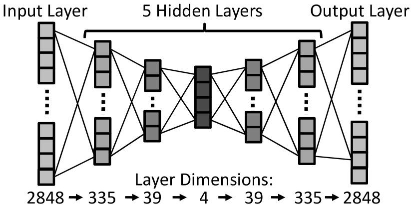
Figure 2. Architecture for Our Autoencoders

Total Traffic Pcaps

Total Traffic Flows

Training

Threshold

Validation

Test

VIPs

Peace Hrs

War Hrs

DDoS Evts

Benign

Malicious

DDoS Evts

Benign

Benign

Benign

Malicious

Benign

Malicious

SR1VP1

110.32

2.31

20

9,930k

119k

20

1,000k

59.5k

59.5k

59.5k

59.5k

59.5k

SR1VP2

96.96

5.44

27

13,107k

1,046k

20

1,000k

523k

523k

523k

523k

523k

SR1VP3

118.88

1.36

49

10,704k

90k

7

1,000k

45k

45k

45k

45k

45k

SR2VP1

57.73

58.89

15

5,469k

37k

10

1,000k

18.5k

18.5k

18.5k

18.5k

18.5k

SR3VP1

182.99

0

0

698k

0

0

548k

50k

50k

0

50k

0

Table 1. Summary of Traffic Pcaps and Traffic Flows Used in This Paper

2.2. Cloud DDoS Data

To evaluate ML-based AD, we obtain peace and war-time traffic packet captures (pcaps) from VIPs on this cloud platform and extract benign user traffic and malicious DDoS traffic.

Cloud VIPs: We study five VIPs from three different services hosted on this cloud platform (see Table 1 for anonymized VIPs). Three of these VIPs (SR1VP1, SR1VP2 and SR1VP3) are instances of a gaming communication service (SR1), each in a different data center and physical location. The other two VIPs (SR2VP1 and SR3VP1) belong to two different gaming authentication services (SR2 and SR3).

Traffic Pcaps: We obtain over 100 hours of inbound traffic pcaps to each of these 5 VIPs. Each VIP’s pcaps include all war-time traffic and partial peace-time traffic, observed at this VIP in a 8-day period between late-May and early-July 2019 (specific times in Table 1). We use partial peace-time traffic because we find more traffic does not increase our models’ accuracy. We observe SR3VP1 for extended 180 hours because this VIP receives less traffic than other VIPs. Our pcaps are sampled, retaining 1 in every 1000 packets.

Our 5 VIPs see different distributions of DDoS events in this period, as in Figure 2. SR1VP3 sees a large number (49) of mostly short DDoS events (71% being 1 second or less, see red crosses in Figure 2). The cloud platform’s DDoS team suggests these brief DDoS events are likely botnets randomly probing IPs. In comparison, SR1VP1 and SR1VP2 see smaller numbers of longer DDoS events, with median durations of 121 and 140 seconds for their 20 and 27 events (Figure 2). SR2VP1 is frequently attacked, with about 59 hours of war time, and sees DDoS events of broad range of durations (from 1 second to more than 14 hours). The cloud’s DDoS team reports that this VIP is hosting a critical service, so long attacks are likely attempts to gain media attention. SR3VP1 reports no DDoS events since service SR3 is rarely attacked. We use SR3VP1 to evaluate false positives with our detection methods.

Benign and Malicious Traffic: We report peace-time traffic as “benign traffic”. While there may be very small attacks in the peace-time traffic, the cloud platform considers any such events too small to impact the service and does not filter them. (We choose to not remove such attacks to evaluate our system on noisy, real-world traffic (Gates06a, ).) War-time traffic is also a mix of benign user traffic and malicious DDoS traffic. We only consider the fraction of war-time traffic dropped by heuristic-based filters from in-house mitigation as malicious (annotated as “malicious traffic” hereafter), recalling these heuristics identify known attacks (§ 2.1). We only use these malicious traffic to evaluate our methods and ignore the rest of war-time traffic since we do not have perfect ground truth for them.

Benign and Malicious Flows: Since our models’ detection relies on flow-level statistics like packet counts and rates, we first aggregate packets from benign and malicious traffic as 5-tuple flows.

We summarize the number of benign and malicious flows and number of DDoS events in these malicious flows in Table 1. Since our malicious flows come from a subset of war-time traffic that matches in-house mitigation’s heuristics, the DDoS events in malicious flows are a subset of DDoS events in war-time traffic pcaps.

Our data is predominantly UDP (99.87% of our 40M flows in Table 1), likely due to all three cloud services we study are latency-sensitive gaming services. We have not evaluated if our results apply to TCP-based services. Future work may relax this limitation.

Extracting Flow Features: We use Argus (argus, ) to extract 23 flow features (see Table 2) from the first 10 seconds (an empirical threshold) of each benign and malicious flow.

Our 23 flow features can be categorized into two groups. The first group of features (ports, rates, and packet sizes, gray in Table 2) are those used in in-house mitigation’s heuristics. These features enables us to understand if our models use the same features in detecting certain malicious flows as in-house mitigation does. Other features (such as flow inter-packet arrival time and packet TTLs, white columns in Table 2) are not used by in-house mitigation, likely because they are less intuitive to humans These features enables us to explore how well ML-AD models could compliment human expertise by using more subtle features in detection.

While many of our features, such as packet rate (Table 2), are distorted by data sampling, we believe our detection still works because our models are trained to identify sampled traffic.

Unordered Feature Encoding: Since three of our features (source port, destination port and protocol) are unordered and directly using them would implicitly create an ordering among their values (for example, implying that port 5 is more similar to port 6 than port 4 is), we use one-hot encoding (one-hot-intro, ) to avoid this distortion. We map protocol into 256 one-hot features (is_protocol_0, is_protocol_1, … is_protocol_255), each with a binary value. Similarly, we map ports into 1286 one-hot features, each representing a group of 51 adjacent ports (1 to 51, 52 to 102, … 65485 to 65535), with port 0 used to indicate both illegal TCP/UDP port 0 and non-existent port in non-TCP-UDP flows. (We group every 51 ports because otherwise we will need 65536$\times$2 one-hot features to represent source and destination ports, more than our machine can handle.) Grouping ports could cause false positives or negatives if two common ports appear in the same aggregate, we examined our data and found that all popular ports differ by at least 53 in the port space and we never group popular ports.

Sport	Dport	Proto	SrcPkts	SrcRate	SrcLoad	SIntPkt	sTtl	sMaxPktSz	sMinPktSz	SrcTCPBase
source	dest	protocol	src-to-dst	src-to-dst	src-to-dst	mean src-to-dst inter	TTL in last src	src-to-dst	src-to-dst	src TCP base
port	port	number	pkt count	pkt/s	bits/s	-pkt arrival time	-to dst pkt	max pkt size	min pkt size	sequence
TcpOpt_{M, w, s, S, e, E, T, c, N, O, SS, D}
the existence of certain TCP option: max segment size (M), window scale (w), selective ACK OK (s), selective ACK (S), TCP echo (e), TCP echo reply (E),
TCP timestamp (T), TCP CC (c), TCP CC New (N), TCP CC Echo (O), TCP src congestion notification (SS) and TCP dest congestion notification (D)

Table 2. Our 23 Flow Features (Merging 12 Features About Existence of Certain TCP Option) Before One-hot Encoding

2.3. DDoS Detection Techniques

Having obtained benign and malicious flows, we next describe the ML models we use and how we train, validate and test these models with these flows. We developed our specific ML-based AD techniques ourselves, but we follow the use of autoencoder like prior work (N-BaIoT, ; autoencoder_anomdet1, ; autoencoder_intrution1, ; autoencoder_outlier1, ) and we specifically follow the idea of N-BaIoT of using reconstruction error to detect DDoS (N-BaIoT, ). Our goal is not to show a new detection method, but to evaluate and interpret current state-of-the-art methods with real world data.

Model Overview: We use a type of neural-network ML model called autoencoder because it is widely used in AD (such as system monitoring (autoencoder_anomdet1, ) and outlier detection (autoencoder_outlier1, )) and has been shown to detect DDoS attacks accurately in lab environment ((N-BaIoT, )). While other ML models are also used for AD, such as one-class SVM (ocsvm1, ; ocsvm2, ; ocsvm3, ) and other neural networks (Chalapathy18a, ; Oza19a, ; DIOT, ; Jun01a, ). We currently focus on autoencoder and leave studying other models for future work.

Autoencoder is a symmetric neural network that reconstructs its input by compressing the input to a smaller dimension and then expanding it back (autoencoder-intro, ). The aim of autoencoder is to minimize reconstruction error, the differences between input and output (the reconstructed input). We compute the difference between input and output vectors ($F_{in}$ and $F_{out}$) as the mean of element-wise square error, as shown in Equation 1 where $N$ is the number of elements in $F_{in}$ and $F_{out}$; and $F_{in}^{i}$ (or $F_{out}^{i}$) is the i-th element in $F_{in}$ (or $F_{out}$).

(1) $$E(F_{in},F_{out})=\frac{\sum_{i=1}^{N}(F_{in}^{i}-F_{out}^{i})^{2}}{N}$$

To detect malicious DDoS flows, we train an autoencoder with only benign flows and identify malicious flows by looking for large reconstruction errors. The rationale is the autoencoder learns to recognize useful patterns in the benign flows with, in-effect, lossy compression. When it encounters statistically different flows like the malicious flows, it cannot compress this anomalous traffic efficiently and so produces a relatively large reconstruction error, with the degree of error reflecting the deviation from normal of the anomaly.

We build a 6-layer neural network for each of our 5 VIPs, compressing a 2848-by-1 input vector (2$\times$1286 one-hot features for ports, 256 one-hot features for protocols and the other 20 features in Table 2) to a 4-by-1 vector and expand it back symmetrically (dimensions of each layer shown in Figure 2). As with many ML systems, the specific choices of 4-by-1 and 6 layers are empirical, although we also tried 8 layers without seeing much advantage. We use ReLu (relu, ) as activation function, L2 regulation (pytorch-weight-decay, ) and dropout (dropout, ) to prevent overfitting and mini-batch Adam gradient descent (adam, ) for model optimization, all following standard best practices (nn_course, ). Our implementation uses pyTorch (pyTorch, ).

Model Training: We train each VIP’s autoencoder to accurately reconstruct benign flows from this VIP.

We first randomly draw 1 million benign flows from each VIP as its training dataset (see “training” column of Table 1). SR3VP1 observes only 698k benign flows, even with extended observation, so there we train on 548k benign flows. (We experimented with additional training data but did not find it helped)

We then pre-process training dataset by normalizing training flows’ feature values to approximately the same scale (about 0 to 1), following best practices (nn_course, ). The one-hot features are already normalized, but for a given other feature $i$ of flow $w$ in the training dataset ($F^{i}_{w}$ in Equation 2), we normalize it with min-max normalization (Equation 2 where $F^{i}_{tmax}$ and $F^{i}_{tmin}$ are the maximum and minimum values for feature $i$ in all training flows).

We initialize four hyper-parameters in our models: mini-batch size as 128, learning rate as $10^{-5}$, drop-out ratio as 50% (per recommendation (dropout, )) and weight decay for L2 regulation ((pytorch-weight-decay, )) as $10^{-5}$. (We tune these values during model validation below if needed.)

Lastly, we train our models with normalized training data for 2 epochs. (Adding more epochs does not increase models’ detection accuracy on validation datasets, and risks overfitting.)

Threshold Calculation: Detecting malicious flows from large reconstruction error requires a threshold to separate normal error from anomalies. We calculate this threshold by estimating the upper bound for benign flows’ errors. We randomly draw benign flows from each VIP to form threshold datasets (see “threshold” column of Table 1). We set the size of threshold dataset to match the size of validation and test dataset (described later this section). Similar to model training, we pre-process threshold data with min-max normalization (Equation 2) and maximum and minimum feature values extracted from training datasets ($F^{i}_{tmax}$ and $F^{i}_{tmin}$). We apply trained models to flows in threshold dataset and record their reconstruction errors as $\mathbb{E}$. We calculate detection threshold with Equation 3 where $\mu_{\mathbb{E}}$ and $\sigma_{\mathbb{E}}$ are mean and standard deviation of $\mathbb{E}$.

(2) $$\hat{F^{i}_{w}}=\frac{F^{i}_{w}-F^{i}_{tmax}}{F^{i}_{tmin}-F^{i}_{tmax}}$$

(3) $$T_{det}=\mu_{\mathbb{E}}+3\sigma_{\mathbb{E}}$$

Model Validation: We validate detection accuracy of trained models (with initial hyper-parameters) by applying them to detect benign and malicious flows in validation datasets. When we encounter poor accuracy in the validation data, we tune hyper-parameters of the models to improve validation accuracy.

To validate our model, we construct validation dataset for each VIP by randomly drawing half malicious flows from a VIP and equal amount of random benign flows from same VIP (shown under “validation” of Table 1). We pre-process validation dataset with min-max normalization and $F^{i}_{tmax}$ and $F^{i}_{tmin}$ (Equation 2). We apply trained models to detect benign and malicious flows in validation sets and check common accuracy metrics of detection results: mainly precision (${\mbox{{TP}}}/({\mbox{{TP}}}+{\mbox{{FP}}})$), recall (${\mbox{{TP}}}/({\mbox{{TP}}}+{\mbox{{FN}}})$) and F1 score (${2\times{\mbox{{precision}}}\times{\mbox{{recall}}}}/({{\mbox{{precision}}}+{\mbox{{recall}}}})$) where TP, FP and FN stands for true positives, false positives and false negatives in identifying malicious flows. Note that for SR3VP1 where we only have benign flows, we instead examine its true negative ratio (TNR, the fraction of benign flows that get correctly detected.)

If any detection metric for a per-VIP model goes under 99%, we tune this model’s hyper-parameters with random search (random_search, ), by training multiple versions of this model, each with a set of randomly-chosen values for hyper-parameters. We then select as the final model the version that gets the highest F1 score against the validation dataset and use this final model for all subsequent detection. (Table 3 lists hyperparamter values for our final models.)

Model Testing: Finally, we report detection accuracy for our trained and validated models by applying them to test datasets, consisting of the other half of malicious flows extracted from each VIP and equal amount of random benign flows from the same VIP (see “Test” of Table 1). Specifically, we first pre-process test dataset with min-max normalization and $F^{i}_{tmax}$ and $F^{i}_{tmin}$ (Equation 2). We then report our models’ detection precision, recall and F1 score on test dataset. (Similar to validation, we report TNR for SR3VP1.)

2.4. Techniques to Interpret Detections

While our models follow best practices, we are the first to evaluate such models with real-world data and interpret the results. We interpret our models’ detection results with feature attribution (§ 2.4.1) and counterfactual explanations analysis (§ 2.4.2).

2.4.1. Feature Attribution

We use feature attribution analysis to understand the contribution from each feature to the detection of each flow instance. Prior work used feature attribution (Zeiler13a, ; zintgraf17a, ; simonyan13a, ; shrikumar16a, ). They either attribute feature importance by evaluating the difference in model output when perturbing each input feature ((Zeiler13a, ; zintgraf17a, )), or by taking the partial derivative of model output to each input feature ((simonyan13a, ; shrikumar16a, )).

(4) $$A(j)=\frac{(F_{in}^{j}-F_{out}^{j})^{2}}{\sum_{i=1}^{N}(F_{in}^{i}-F_{out}^{i})^{2}}$$

Since our models’ detection is based on reconstruction error of input flow (Equation 1), which is the mean of per-feature errors from all flow features, we can measure a feature’s contribution to detection by how much error it contributions to overall reconstruction error. We normalize per-feature error by dividing it with the sum of error from all features, as in Equation 4, and attribute that feature’s contribution as this normalized per-feature error.

2.4.2. Counterfactual Explanations

Counterfactual explanations show how an input must change to significantly change its detection output, as advocated by prior work (wachter17a, ; Martens14a, ).We use counterfactual explanations to understand the normality our models learn for each flow feature, suggesting values the models consider anomalous.

Specifically, we first find a base flow that is detected as benign, then we repeatedly alter the target feature’s value in this base flow while keeping other features unchanged. We feed these altered base flows into our model to observe how much the reconstruction error changes with each perturbation of target feature’s value: an increase in errors suggests our models consider current feature value more abnormal than the previous value, and vice versa. We repeat this experiment on different base flows to see if our models consistently consider certain target feature values more normal than the other values, with relatively normal values suggesting normality our models learned.

3. Detection Results

	Mini-batch Size	Learning Rate	Drop-out Ratio	Weight Decay
SR1VP1	64	$2\times 10^{-5}$	10%	$10^{-6}$
SR2VP1	32	$10^{-5}$	10%	$2\times 10^{-6}$
Other VIPs	128	$10^{-5}$	50%	$10^{-5}$

Table 3. Hyperparameters Values for Final Models

To understand how well ML-based AD works in detecting real-world DDoS attacks, we train and validate an autoencoder model for each of our 5 VIPs as described in § 2.3. We summarize hyperparameters values for our final models in Table 3 where models for SR1VP1 and SR2VP1 use tuned hyperparameters values and models for other 3 VIPs use initial hyperparamter values from § 2.3.

With trained and validated models, we report detection accuracy on test datasets in § 3.1 and examine false positives in § 3.2. In § 3.3, we evaluate our models on all malicious flows (recalling test datasets only contain half of total malicious flows) and interpret why our models detect some malicious flows but miss others in § 4.

3.1. Detection Accuracy on Test Dataset

We evaluate accuracy by measuring precision, recall, F1 score and TNR of our models’ detection of test datasets in Table 4.

We first observe that our model’s detection precision and TNR for all 5 VIPs are high (at least 98.90% in Table 4), suggesting they rarely generate false alerts: only 2,556 (0.36%) false positives out of all 696,000 tests of benign flows. (We later show that only 28 of these 2,556 are actual false positives in § 3.2.)

	SR1VP1	SR1VP2	SR1VP3	SR2VP1	SR3VP1
Precision	98.90%	99.69%	99.81%	99.50%	–
Recall	94.75%	99.99%	100.0%	91.37%	–
F1-Score	96.78%	99.83%	99.90%	95.26%	–
TNR	–	–	–	–	99.68%

Table 4. Detection Accuracy on Test Dataset

Our second observation is that our models identify almost all malicious flows to 2 of the 4 VIPs under attack (detection recall is 99.99% for SR1VP2 and 100% for SR1VP3) and identify most malicious flows to the other 2 VIPs (recall is 94.75% for SR1VP1 and 91.37% for SR2VP1), as shown in Table 4.

3.2. Examining False Positives on Test Dataset

Our models make 2,556 false positives against the test datasets (§ 3.1); we next compare these to in-house mitigation’s heuristics such as allow-lists of destination ports and protocols.

We first show most of these false positives (95.7%, 2,446 out of 2,556, see Table 5) are actually true positives (correctly-detected malicious flows), recalling our noisy training data may contain some malicious traffic (§ 2.2). We find most of these actual true-positive flows (79.8%, 1,953 out of 2,446) are UDP flows with malicious destination ports. We also find a small fraction of them using malicious source ports (0.2% or 4), and a few with at least one packet with bad payload content (that fails regular expressions required by in-house mitigation’s heuristics) (0.1% or 2). (We show in § 4.3 that our models could detect some malicious flows with bad packet payload content based on anomalies in flow features.)

We next show a few false positives (3.2%, 82 out of 2,446) are artifacts due to misdirected TCP flows (Table 5). These misdirected flows appear to originate from our 5 VIPs, yet the pcaps we study contain only inbound packets to these VIPs (§ 2.2). These misdirected flows thus have wrong values of zeros for some of our features such as source-to-destination packet counts and rates (Table 2). We confirm that these flows’ directions are actually mis-labeled due to a known limitation of Argus.

Lastly, we show the remaining 28 false positives are likely actual false positives. Each of them (all TCP flows) does not match any of in-house mitigation’s heuristics.

We conclude that only a tiny fraction of false positives reported in § 3.1, are actual false positives (1.1%, 28 out of 2,556), suggesting the actual false positive rate is near zero (0.00%, 28 of 696,000 test benign flows). (We explore the potential causes for these actual false positives in § 4.2.)

total false positives	2,556	(100.0%)
actual false positives	28	(1.1%)
actual true positives	2,446	(95.7%)	(100.0%)
UDP flows w bad dst port	1,953	(76.5%)	(79.8%)
UDP flows w bad src port	4	(0.2%)	(0.2%)
UDP flows w bad payload content	2	(0.1%)	(0.1%)
flows w bad protocols	487	(19.1%)	(19.9%)
misdirected TCP flows	82	(3.2%)

Table 5. False Positives on Test Dataset Breakdown

3.3. Detection Accuracy On All Malicious Flows

We next explore how well our models detect all malicious flows we have, recalling test datasets contain only half of them (§ 2.3). We group malicious flows by their main anomalies as detected in-house mitigation, and show which anomalies are best detected by our models, and which are poorly detected.

Our models are near perfect at detecting anomalies on allow-listed features (those with mostly malicious values besides a few benign values, judged by in-house mitigation’s heuristics) with unordered values: destination port and protocol. As a result, our models capture all flows with malicious protocol (100.00% of about 15k) and nearly all UDP flows with malicious destination ports (99.92% of about 1M), see Table 6.

Our models are reasonable at detecting anomalies on deny-listed features (those with mostly benign values besides a few malicious values, judged by in-house mitigation’s heuristics) with unordered values: source port. Our models identify most UDP flows with malicious source ports (97.5% of 5k).

However, we find our models are bad at detecting anomalies on deny-listed features with ordered values: flow packet sizes. Our models detect only a few malicious flows (8.5% of about 3k) containing packets with too-small payload (in-house mitigation drops UDP packets with payload smaller than a threshold), as in Table 6. (In § 4.1, we show that our models infer if a UDP flow contains packets with too-small payloads based on feature maximum and minimum flow packet size, recalling Table 2.)

Lastly, our models detect a quarter of UDP flows (24.7% of 8k) containing packets with bad payload contents (that fail regular expressions required by in-house mitigation), despite our models do not see packet payloads (Table 6).

Total Flows by Main Anomalies		Detected Flows
Main Anomaly	Count	Count	Frac of Total
Flows w Bad Protocol	15,206	15,206	100.00%
UDP Flows w Bad Dst Port	1,261,951	1,260,943	99.92%
UDP Flows w Bad Src Port	5,334	5,201	97.5%
UDP Flows w Too Small Payload	2,522	215	8.5%
UDP Flows w Bad Payload Contents	8,229	2,036	24.7%

Table 6. Detection to All Malicious Flows Breakdown

4. Interpreting Detection of Malicious Flows

No.	Descriptions
1	Autoencoder can be trained successful with noisy data (§ 3), provided all benign values of target feature appear frequently in this data (§ 4.1)
2	Autoencoder can reliably detect anomalies on features whose benign values are frequent among training data (§ 4.1) and who are also unordered (§ 4.2)
3	Autoencoder almost always combines anomalies from multiple features in detection (§ 4.3), using even features that are less intuitive for human (§ 4.2)

Table 7. Key Takeaways from Interpretation Results

A contribution of our work is to interpret why ML-based AD detects certain anomalies better than others. We show that our models are better at detecting anomalies on allow-listed features than those on deny-listed features because they are more likely to learn correct normality for allow-listed features (§ 4.1). Our models are better at detecting anomalies on unordered features than those on ordered features because even with incomplete normality, our models could still detect anomalies on unordered feature with high recall (§ 4.2). Lastly, our models detect anomalies on packet payload content by combining multiple flow features (§ 4.3).

We summarize key takeaways from our interpretation results in Table 7 and describe our interpretation results’ implications on using autoencoder-based AD in production later in § 5.

4.1. Learning Normalities for Features

We show our models are more likely to learn correct normality for allow-listed features (destination port and protocol) than for deny-listed features (source port and flow packet sizes). The rationale is that since our models learn frequently seen values in training data as normality, it is more likely for allow-listed features to have all their benign values frequently seen in training data and thus learned as normality because they have, by definition (§ 3.3), only a few benign values. (We show how the normalities learned affect our detection of anomalies later in § 4.2.)

Allow-listed Destination Port: We show our models correctly learn normality for destination port (with all values being malicious except one benign value, per in-house mitigation’s heuristics) because the one benign port is the most frequent among training data.

We explore the normality our models learn for destination ports with counterfactual explanation (§ 2.4.2). We randomly draw 100 UDP flows, detected as benign, from each VIP’s test datasets as base flows, alter these 500 base flows by enumerating their destination ports from 0 to 65535 with a step size of 51 (0, 51, … 65535) and feed altered flows into models. The step size is because our models merge each 51 adjacent ports to one feature (§ 2.2). We then watch for how base flows’ errors change as destination ports change.

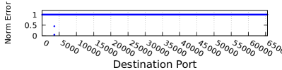
Figure 3. Normalized Reconstruction Errors for 100 Base Flows from SR1VP2 using Different Destination Ports

We show our models correctly learn the normality of destination ports by consistently considering base flows with malicious ports more abnormal than the same flows with the one benign port. We use reconstruction errors from SR2VP1’s 100 base flows as example (other VIPs are similar). Since we only care about how a base flow’s error changes as its destination port changes (rather than the exact values of these errors) and want to compare these changes across all 100 base flows from this VIP, we normalize the set of errors resulted from one base flow using different destination ports to range $[0,1]$ by dividing these errors with the maximum error found among them. We plot normalized errors for SR2VP1’s 100 base flows with different destination ports as blue dots in Figure 3. We show that all malicious ports lead to similarly high reconstruction errors and this pattern is very consistent across all 100 base flows from SR2VP1 (represented by the horizontal blue line at normalized error 1 in Figure 3). We also show consistently low errors (at most 0.46) at the one benign port for SR2VP1 (shown as the blue dots to the left of port 5000 and below error 0.5 in Figure 3).

Allow-listed Protocol: We show our models learn incomplete normality for protocols. Per in-house mitigation’s heuristic, all protocols are malicious except UDP (for SR1, SR2 and SR3), TCP (for SR1 and SR3) and 3 other protocols (for SR3 only, exact protocols omitted for security). However our models only learn UDP as benign because the other 4 protocols are infrequent in training data.

We explore normality our models learn for protocols by applying counterfactual explanation to the same 500 base flows from destination port analysis, varying their protocols from 0 to 255 (with a step size of 1) and watch for how their reconstruction error changes.

We show our models learn incomplete normality for protocols by consistently considering based flows with non-UDP protocols more abnormal than same flows with UDP. For example, in SR3VP1’s normalized errors (Figure 4), we find blue dots representing UDP (at protocol 17) consistently correspond to low errors (at most 0.56). (Other 4 VIPs are similar.)

Figure 4. Normalized Reconstruction Errors for 100 Base Flows from SR3VP1 using Different Protocols

We believe that our models fail to learn non-UDP benign protocols because they are infrequent in training data. While UDP accounts for almost all training data for our 5 VIPs (99.87% of 4.5M), TCP accounts for only a tiny fraction (0.01% of 4.5M) and the 3 other benign protocols for SR3 are completely missing. We note that TCP flows show up even less than noises in training data (flows with malicious protocols, showing up in 0.11% of 4.5M), suggesting that it actually makes sense for our models to ignore infrequent benign protocols like TCP otherwise it risks learning noises.

Figure 5. Normalized Reconstruction Errors for 100 Base Flows from SR2VP1 using Different Source Ports

Deny-listed Source Port: We show our models are unlikely to learn correct normality for deny-listed features like source port because their values are mostly benign (per definition § 3.3) and it is unlikely for all their benign values to be frequently seen in training data and learned as normality.

We explore normalities our models learn for source port by applying similar counterfactual explanation analysis as we do for destination port.

We show our models fail to learn the correct normality for source ports. Per in-house mitigation’s heuristic, most source ports are benign (besides 1024 and 1023 malicious ports) for SR1 and SR2 and all source ports are benign for SR3. However, our models only consider a few source ports frequently seen in training data (“frequent training ports”) as relatively normal. As an example, we show reconstruction errors of SR2VP1’s 100 base flows in Figure 5. (We summarize results for other 4 VIPs later.) We find for SR2VP1, source port 3111 (blue dots left of port 5000 and below error 0.5 in Figure 5) consistently lead to low errors (at most 0.38) while the rest ports lead to high errors (see horizontal blue line at error 1). We believe the reason for port 3111’s low errors is that it corresponds to benign source port 3074 which is the most frequent among SR2VP1’s training data, (in 75.31% of 998k training UDP flows), considering our models do not distinguish among port 3061 to 3111 due to our grouping of adjacent 51 ports during one-hot encoding (§ 2.2). We find similar trend in reconstruction errors for other 4 VIPs: low error with the most frequent training source port (all benign) and high errors with the rest source ports. The only exception is that we find one malicious source port for SR1VP1 (omitted for security) also leads to low error due to it is the second most frequent among SR1VP1’s training data (in 1.21% of 999k UDP training flows, recalling our training data is noisy). We conclude that our models learn incorrect normality for SR1VP1 (considering one benign and one malicious source ports normal) and incomplete normality for other 4 VIPs (considering one benign port normal).

Deny-listed Packet Sizes: Similarly, our models are not likely to learn correct normality for deny-listed flow packet sizes.

Our models detect malicious flows with too-small-payload UDP packets (Table 6), without actually seeing packet payload, by identifying malicious combinations of sMaxPktSz and sMinPktSz (maximum and minimum flow packet sizes, see Table 2). The rationale is that we find malicious flows with too-small-payload UDP packets in our data for SR2VP1 (other VIPs do not filter on payload sizes) are either made of all 56 or all 60-byte packets. As a result, these malicious flows have only two possible combinations of sMaxPktSz and sMinPktSz (both 56 or both 60). Since these two sMaxPktSz and sMinPktSz combinations are rare among SR2VP1’s UDP training flows (0.01% of 998M, not bad comparing to, for example, 0.46% noises for benign destination ports), detecting flows with too-small-payload packets is equivalent to detecting flows with malicious sMaxPktSz and sMinPktSz combinations (both 56 and both 60).

(a) SR1VP1 (normal when both small)

(b) SR2VP1 (normal when similar)

(c) SR3VP1 (normal when both large)

Figure 6. Reconstruction Errors (Unit: $T_{det}$ from Equation 3) for 1 Base Flow from 3 VIPs with Varying Packet Sizes (Byte)

Figure 7. Frequent sMaxPktSz (X axis) and sMinPktSz (Y axis) Combinations in Training UDP Flows (At Least 1000 Occurrence).

We study the normality our models learn for sMaxPktSz and sMinPktSz combinations with counterfactual explanation. We randomly draw 10 base flows from each of our 5 VIPs’ test dataset, vary sMaxPktSz and sMinPktSz in base flows from 0 to 512 bytes (the largest packet size in our data) with a step size of 1 and watch how base flows’ errors change.

We show our models learn incomplete normality for sMaxPktSz and sMinPktSz combinations, by considering frequent combinations in training data, instead of all benign combinations (all except both 56 and both 60 for SR2VP1 and all combinations for other 4 VIPs), as relatively normal. Our models for SR1’s three VIPs consider base flows relatively normal when sMaxPktSz and sMinPktSz are both small (6(a) shows reconstruction errors of one base flow from SR1VP1) because they mostly see small sMaxPktSz and sMinPktSz (at most 104 bytes) in training data (Figure 7). The only exception is that we find a few training UDP flows for SR1VP1 (about 1.42% of 999M) have large sMaxPktSz and sMinPktSz (both 512 bytes, see blue pluses on top right corner of SR1VP1 chart in Figure 7). However our model for SR1VP1 still considers sMaxPktSz and sMinPktSz of both 512 abnormal (see the red on top right corner of 6(a)), likely treating these training flows as noises. Our model for SR2VP1 considers base flows relatively normal when sMaxPktSz and sMinPktSz are similar in value (6(b) shows reconstruction errors for one base flow from SR2VP1) because it mostly sees similar sMaxPktSz and sMinPktSz (both from 74 to 512 bytes) in training data (Figure 7). Our model for SR3VP1 considers base flows relatively normal when sMaxPktSz and sMinPktSz are both large (6(c) shows reconstruction errors for one base flows from SR3VP1) because it mostly see large sMaxPktSz and sMinPktSz (at least 397 bytes) in training data (Figure 7).

4.2. Detecting Anomalies on Features

We next show that with correct normality, our models achieve reliable detection for anomalies on unordered feature (destination port). With incomplete normalities, our models stills detect anomalies on unordered features (protocol and source port) with high recall but risk false positives. Lastly, we show that incomplete normalities could lead to low-recall detections for anomalies on ordered features (flow packet sizes).

Unordered Destination Port: We show that the correct normality our models learn for destination port is key to the reliable detection of almost all flows with malicious destination ports (99.92%; 1,260,943 out of 1,261,951, from Table 6). Feature attribution analysis (§ 2.4.1) confirms that most (98.55%) of these true-positive detections are mainly triggered by anomalies from destination ports, providing in average $0.80\times$ threshold of reconstruction errors. For the rest reconstruction errors (in average $0.20\times$ threshold) needed, our models rely on anomalies on other features (mainly Sport, sMaxPktSz, sMinPktSz and SIntPkt from Table 2, with at least 10% attributions in from 84% to 3.53% of these detections).

We argue that the tiny fraction of flows with malicious destination ports that our models miss (0.08%, see Table 6) are artifacts of our one-hot encoding of destination port rather than actual false negatives of our models’ detection. Recalling our models can not distinguish among adjacent 51 destination ports since we group them as one one-hot feature (§ 2.2), our models consider these flows benign because their malicious destination ports are adjacent to the benign port (within 51).

Unordered Protocol: Despite learning incomplete normality, we show our models still detect all 15,206 flows (Table 6) with malicious protocols (all except UDP, TCP and three other protocols, recalling § 4.1) by simply considering all flow with non-UDP protocol as equally abnormal (see the horizontal blue line at normalized error of 1 for all non-UDP protocols in Figure 4). Feature attribution confirms that these true-positive detections are completely triggered by anomalies from protocols.

However by considering all non-UDP protocols equally abnormal, our models risk flagging flows with non-UDP benign protocols (such as TCP for SR1 and SR3) as malicious (false positives). causing the 28 false-positive detections our models made on test dataset (all TCP flows), recalling § 3.2.

Unordered Source Port: Similarly, our models detect most flows with malicious source ports (5,201 out of 5,334, 97.5%, recalling Table 6), despite failing to learn the correct normalities, by considering all infrequent training source ports (including all but one malicious ports for SR1VP1 and all malicious ports for other 4 VIPs) equally abnormal. While our models risk false-positive detection by considering benign source ports that are infrequent in training data as relatively abnormal, we see no such false positives in test data (as shown in § 3.2).

Feature attribution analysis confirms that most (99.79%) of these true-positive detections are mainly triggered by anomaly from source ports, providing in average about 0.79$\times$ threshold of reconstruction errors. For the remaining reconstruction error needed (in average about 0.21$\times$ threshold), our models rely on anomaly from additional features (mainly sMaxPktSz, sMinPktSz, SIntPkt, SrcPkts, TcpOpt_M and sTtl from Table 2, with at least 10% attribution in from 85.63% to 1.6% of these detections.)

We note that none of our models’ 133 false-negative detection are due to they incorrectly consider one malicious source port from SR1VP1 as relatively normal (recalling § 4.1). These false negatives are all due to our models cannot find enough anomalies from additional features (besides source ports) to trigger detection.

Ordered Packet Sizes: We show that with incomplete normality for ordered features, our models risk low-recall detections. While for unordered features like ports and protocols, our models consider values different from frequent training values as equally abnormal, our models consider values of ordered features that are more different from frequent training values as more abnormal (see the gradual color changes from blue on left bottom to red on top right in 6(a) as an example). As a result, our models risk considering malicious values for ordered features as relatively normal if they happen to be numerically close to the frequent training values.

We show that with incomplete normality, our model for SR2VP1 incorrectly consider the malicious sMaxPktSz and sMinPktSz combinations (both 56 and both 60 bytes) as relatively normal (shown as the blue bottom left corner of 6(b)) because these malicious combinations happen to be numerically close to some frequent training combinations (both 74 bytes, as shown in SR2VP1’s chart in Figure 7). As a result, our models only detect a few flows with these malicious combinations (8.5%, 215 out of 2,522, from Table 6). Feature attribution analysis confirms that in these 215 true-positive detections, our model almost exclusively relies on anomalies from features other than sMaxPktSz and sMinPktSz.

4.3. Using Anomalies from Multiple Features

Lastly, we show that our models almost always combine anomalies from multiple flow features in detection, enabling our models to detect a quarter UDP flows with malicious packet payload contents (24.7%, 2,036 out of 8,229, in Table 6) even when they cannot see packet payload contents. We breaking down number of features with significant attributions (at least 10%) in our models’ detection of all 1.2M malicious flows in Table 6 and show that our models uses multiple significantly-attributing features in nearly all detections (99.90% of 1.2M) and uses 4 in most detections (79.16% of 1.2M).We argue that combining anomalies from multiple features is actually necessary for our models’ detection by showing that almost all of these detected malicious flows would be missed (97.15% of 1.2M) if only using anomalies from the highest attributing features.

5. Findings and Implications

We next distill our interpretation results to three implications: training with noisy real-world data is possible (§ 5.1), autoencoder can reliably detect real-world anomalies on well-represented unordered features (§ 5.2) and combinations of autoencoder-based AD and heuristic-based filters can help both (§ 5.3).

5.1. Training with Noisy Data is Possible

Our results show autoencoder-based AD models can be trained successfully on real-world data with noises, provided target features are well-represented: all benign values of target feature must appear frequently in the training data. Our results support prior claim that attack-free training data does not exist outside simulation (Gates06a, ) (we find some brief attacks in our training data), but we disprove the claim that noisy data makes AD training impossible.

We prove this ability to train on noisy data, showing that our autoencoder-based AD can learn normality in spite of noise. For example, our models learn correct normality of destination port despite noise in the training data (0.46% of 4.5M UDP flows have malicious destination port) because the benign port is the most frequent in training data (99.54% of 4.5M UDP flows), recalling § 4.1.

We also show that for under-represented features, noise can be confused with normality, because both noise and some of their benign values are infrequent. For example, in § 4.1, our models fail to learn benign protocol TCP (in 0.01% of training flows) as normal likely due to our models consider TCP as noises, considering actual noises (in 0.22% of training flows) are more frequent than TCP. Our model for SR1VP1 learns a malicious source port (noise) as normal because this port is the second most frequent in training data (in 1.21% of training UDP flows) and is more frequent than almost all benign sort ports.

5.2. Autoencoder Reliably Detects Anomalies on Well-represented Unordered Features

Our results suggest that autoencoder-based AD could reliably detects real-world DDoS attacks, but only when all benign values for the DDoS flow’s anomalous feature appear frequently in training data (so that our models could learn these benign values as normal) and when this anomalous feature is unordered (so that our models could crisply infer all the other values as abnormal). If some benign values for this anomalous feature are infrequent in training data (as is usually the case for deny-listed features), our models risk considering these benign values as abnormal (false positives). If this feature is ordered (such as packet rates, counts and sizes), even when all of its benign values appear frequently in training data, our models still risk considering malicious values numerically close to these benign values as normal (false negatives).

Our results thus refute the claim from prior work based on lab traffic that autoencoder-based AD detects DDoS attacks reliably (with true positive rate of 100% and false positive rate of near 0) (N-BaIoT, ). Our results suggest that an autoencoder-based AD will not detect sufficient attacks if it is the only DDoS-detection method in production environment. We instead recommend using autoencoder-based AD as a compliment to heuristic-based DDoS filters, see § 5.3.

5.3. Combine AD and Heuristic-Based Filters

Finally, we show the potential for joint use of autoencoder-based AD and heuristic-based filters (like in-house mitigation), since each has its own strengths.

We find our models are very good at finding and using anomalies from multiple features (4 in detection to most malicious flows § 4.3). ML-based AD is particularly important when the anomalies are not obvious to human perception, such as anomalies in flow inter-packet arrival time, packet count and packet TTLs (recalling § 4.2). However, our models are not very certain about each one of these anomalies and would miss 97.15% of its detected malicious flows if only using the highest-attributing feature (§ 4.3).

The heuristic-base filter, by relying on human expertise, is very good at detecting malicious flow based on single anomaly. (While in-house mitigation uses multiple heuristic-based filters, only one filter is used in each detection: the highest-priority filter triggered.) For example, a flow with malicious destination port is certainly malicious because the server only serves a short list of benign ports. However we argue that it is more challenging for heuristic-based filters to make use of more subtle features to indicate malice, such as flow inter-packet arrival time or packet TTLs. Our models are able to make use of these features (§ 4.2), and can combine multiple suggestive features (§ 4.3).

We propose two possible strategies to combine autoencoder-based AD and heuristic-based filters. The first is to simply stack them: apply the heuristic filter first, to cover intuitive anomalies with great certainty. Then add ML-based AD to covering additional anomalies that are not obvious or require combinations of features. Our second strategy is to build new heuristics based on interpretations of what the autoencoder-based AD has discovered, as discussed in § 4. Such “ML-discovered” filters could directly use the ML model, or we could extract the relevant features into a new implementation.

6. Related Work

To the best of our knowledge, we are the first attempt to address the two limitations (limited evaluation dataset and no detection interpretations) in prior DDoS detection study using ML-based AD.

6.1. DDoS Study using ML-based AD

The most related class of prior work are those also detect DDoS attacks with ML-AD models.

Most prior work in this class train some form of ML-AD models, such as one-class SVM models ((ocsvm1, ; ocsvm2, ; ocsvm3, )) and neural network models ((N-BaIoT, ; DIOT, ; DIOT, )) with benign traffic and detect attacks by looking for deviations from these benign traffic. Since these prior work mostly test their models with limited datasets including simulation (ocsvm3, ; Jun01a, ), lab traffic (ocsvm1, ; ocsvm2, ; N-BaIoT, ; DIOT, ) and DARPA/MIT dataset (ocsvm1, ), it is not clear how well their methods could work in real-world production environment ((Gates06a, ; Sommer10a, )). Moreover, they usually do not interpret their models’ detection decision nor explore why their models work or not work in detecting certain DDoS attacks. In comparison, we evaluate our models with real-world benign and attack traffic from a major cloud provider and interpret why our models work well on attacks of certain anomalies but not as well on the others.

K-means (kmean, ) and single-linkage (singlelinkage, ) have previously been used as clustering algorithms to separate benign and malicious traffic flows into different clusters. Although their detection results are intuitively interpretable (a flow is flagged as malicious since its features are qualitatively close to features of other flows in the “malicious cluster”), they rely on manual inspection to determine which clusters are malicious. They also evaluate their methods with limited datasets (lab data (kmean, ) and KDD datasets (singlelinkage, )). In comparison, we do not rely on manual inspection for our detection, and we test our methods on real-world traffic from a large cloud platform.

6.2. DDoS Study using Other Techniques

Many prior work detect DDoS attacks with other techniques. We classify them into following 3 classes.

ML-based binary classification: This class of papers train some form of ML binary classification models (such as KNN (nn6, ), decision tree (decesion_tree1, ; nn6, ), two-class SVM (tcsvm1, ; tcsvm2, ), random forest (nn6, ) and neural network models (nn1, ; nn2, ; nn3, )) with both benign and attack traffic. These ML models thus identify attacks similar to the ones they have seen during training. In comparison, we focus on a different model (ML-AD model) and by training with only benign traffic and looking for deviations from these benign traffic, our models do not rely on on knowledge of known attacks and have the ability to identify potential unknown attacks.

Statistical AD: This class of papers apply statistical models (such as adaptive threshold (adathre1, ), cumulative sum (cusum1, ; adathre1, ), entropy-based analysis (entropy1, ) and Bayesian theorem (Bayesian1, )) to identify abnormal traffic pattern that is significantly different from some or all of previously seen (benign) traffic pattern. These papers thus could also cover potentially unknown attacks. In comparison, we focus on AD based on ML models instead of statistical models.

Heuristic-based rule: This class of papers use heuristic-based rules to detect specific types of attacks matching their heuristics. For example, history-based IP filtering remembers frequent remote IPs during peace time and consider traffic from other IPs during attack time as potential DDoS traffic (hurestic1, ). Hop-count based filtering identifies spoofed DDoS packets by remembering peace-time IP to (estimated) hop count mapping and considering packets with unusual IP-to-hop-count mapping during attack time as spoofed DDoS packets (hurestic2, ). In comparison, we use a different method (ML-based AD) and could cover many different types of attacks instead of only a specific type.

7. Conclusion

This paper addresses two limitations in prior studies of ML-based AD: use of real-world data, and interpretation of why the models are successful. We apply autoencoder-based AD to 57 real-world DDoS events captured at 5 VIPs of a large commercial cloud provider. We use feature attribution and counterfactual techniques to explain when our models work well and when they do not. Key results are that our models detect most, if not all, malicious flows to 4 VIPs under attacks, with near-zero false positives. Interpretation shows our models are better at detecting anomalies on allow-listed features than those on deny-listed features because our models are more likely to learn correct normality for allow-listed features. We then show that our models are better at detecting anomalies on unordered features than those on ordered features because even with incomplete normality, our models could still detect anomalies on unordered feature with high recall. Key implications of our work are that training with noisy data is possible, that autoencoder-based AD can reliably detect anomalies on well-represented unordered features and that autoencoder-based AD and heuristic-based filters have complementary strengths.

References

- [1] J. Bergstra and Y. Bengio. Random search for hyper-parameter optimization. Journal of Machine Learning Research, 2012.
- [2] A. Borghesi, A. Bartolini, M. Lombardi, M. Milano, and L. Benini. Anomaly detection using autoencoders in high performance computing systems. CoRR, abs/1811.05269, 2018.
- [3] R. Chalapathy, A. K. Menon, and S. Chawla. Anomaly detection using one-class neural networks. CoRR, abs/1802.06360, 2018.
- [4] J. Chen, S. Sathe, C. Aggarwal, and D. Turaga. Outlier detection with autoencoder ensembles. In Proceedings of SIAM International Conference on Data Mining, 2017.
- [5] Cynthia Wagner, Jérôme François, Radu State, and Thomas Engel. Machine learning approach for IP-flow record anomaly detection. In Proceedings of IFIP Networking Conference, 2011.
- [6] R. Doshi, N. Apthorpe, and N. Feamster. Machine learning ddos detection for consumer internet of things devices. CoRR, abs/1804.04159, 2018.
- [7] C. Gates and C. Taylor. Challenging the anomaly detection paradigm: A provocative discussion. In Workshop on New Security Paradigms, 2007.
- [8] GeeksforGeeks. One-hot encoding introduction. https://www.geeksforgeeks.org/ml-one-hot-encoding-of-datasets-in-python/.
- [9] D. Hu, P. Hong, and Y. Chen. FADM: DDoS flooding attack detection and mitigation system in software-defined networking. In IEEE GLOBECOM, 2017.
- [10] L. Jun, C. N. Manikopoulos, J. Jorgenson, and J. L. Ucles. HIDE: a hierarchical network intrusion detection system using statistical preprocessing and neural network classification. In Workshop on Information Assurance and Security, 2001.
- [11] K. Kato and V. Klyuev. An intelligent ddos attack detection system using packet analysis and support vector machine. Intelligent Computing Research, 2014.
- [12] Y. Kim, W. C. Lau, M. C. Chuah, and H. J. Chao. PacketScore: A statistics-based packet filtering scheme against distributed denial-of-service attacks. IEEE Transactions on Dependable and Secure Computing, 2006.
- [13] D. P. Kingma and J. Ba. Adam: A method for stochastic optimization, 2014.
- [14] M. L. Lab. DARPA/MIT dataset. https://www.ll.mit.edu/r-d/datasets.
- [15] X. Ma and Y. Chen. DDoS detection method based on chaos analysis of network traffic entropy. IEEE Communications Letters, 2014.
- [16] D. Martens and F. Provost. Explaining data-driven document classifications. MIS Quarterly, 2014.
- [17] Y. Meidan, M. Bohadana, Y. Mathov, Y. Mirsky, A. Shabtai, D. Breitenbacher, and Y. Elovici. N-BaIoT—network-based detection of IoT botnet attacks using deep autoencoders. IEEE Pervasive Computing, 2018.
- [18] Y. Mirsky, T. Doitshman, Y. Elovici, and A. Shabtai. Kitsune: An ensemble of autoencoders for online network intrusion detection, 2018.
- [19] V. Nair and G. E. Hinton. Rectified linear units improve restricted boltzmann machines. In International Conference on Machine Learning, 2010.
- [20] T. D. Nguyen, S. Marchal, M. Miettinen, M. H. Dang, N. Asokan, and A. Sadeghi. DÏoT: A crowdsourced self-learning approach for detecting compromised IoT devices. CoRR, abs/1804.07474, 2018.
- [21] P. Oza and V. M. Patel. One-class convolutional neural network. CoRR, abs/1901.08688, 2019.
- [22] T. Peng, C. Leckie, and K. Ramamohanarao. Proactively detecting distributed denial of service attacks using source IP address monitoring. In International Conference on Research in Networking, 2004.
- [23] L. Portnoy. Intrusion detection with unlabeled data using clustering. Thesis, 2010.
- [24] PyTorch. PyTorch project front page. https://pytorch.org.
- [25] PyTorch. Weight decay for Adam. https://pytorch.org/docs/stable/optim.html.
- [26] Qosient. Argus- auditing network activity. https://qosient.com/argus/.
- [27] A. Saied, R. E. Overill, and T. Radzik. Artificial neural networks in the detection of known and unknown DDoS attacks: Proof-of-concept. In Highlights of Practical Applications of Heterogeneous Multi-Agent Systems. The PAAMS Collection, 2014.
- [28] S. Seufert and D. O’Brien. Machine learning for automatic defence against distributed denial of service attacks. In IEEE ICC, 2007.
- [29] N. Shone, T. N. Ngoc, V. D. Phai, and Q. Shi. A deep learning approach to network intrusion detection. IEEE Transactions on Emerging Topics in Computational Intelligence, 2018.
- [30] A. Shrikumar, P. Greenside, A. Shcherbina, and A. Kundaje. Not just a black box: Learning important features through propagating activation differences, 2016.
- [31] K. Simonyan, A. Vedaldi, and A. Zisserman. Deep inside convolutional networks: Visualising image classification models and saliency maps, 2013.
- [32] C. Sinclair, L. Pierce, and S. Matzner. An application of machine learning to network intrusion detection. In Proceedings of ACSAC, 1999.
- [33] V. A. Siris and F. Papagalou. Application of anomaly detection algorithms for detecting syn flooding attacks. In IEEE GLOBECOM, Nov 2004.
- [34] R. Sommer and V. Paxson. Outside the closed world: On using machine learning for network intrusion detection. In Proceedings of IEEE Symposium on Security and Privacy. IEEE Computer Society, 2010.
- [35] N. Srivastava, G. Hinton, A. Krizhevsky, I. Sutskever, and R. Salakhutdinov. Dropout: A simple way to prevent neural networks from overfitting. Journal of Machine Learning Research, 2014.
- [36] Stanford. CS231n. http://cs231n.github.io/.
- [37] Stanford. DL tutr. http://ufldl.stanford.edu/tutorial/unsupervised/Autoencoders/.
- [38] Taeshik Shon, Yongdae Kim, Cheolwon Lee, and Jongsub Moon. A machine learning framework for network anomaly detection using svm and ga. In IEEE SMC Information Assurance Workshop, 2005.
- [39] Tao Peng, C. Leckie, and K. Ramamohanarao. Protection from distributed denial of service attacks using history-based ip filtering. In IEEE ICC, 2003.
- [40] D. S. Terzi, R. Terzi, and S. Sagiroglu. Big data analytics for network anomaly detection from netflow data. In UBMK, 2017.
- [41] UCI. KDD cup dataset. https://kdd.ics.uci.edu/databases/kddcup99/.
- [42] S. Wachter, B. Mittelstadt, and C. Russell. Counterfactual explanations without opening the black box: Automated decisions and the gdpr, 2017.
- [43] H. Wang, C. Jin, and K. G. Shin. Defense against spoofed ip traffic using hop-count filtering. IEEE/ACM Transactions on Networking, 2007.
- [44] I. H. Witten and E. Frank. Data Mining: Practical Machine Learning Tools and Techniques with Java Implementations. Morgan Kaufmann, 2005.
- [45] J. Yu, H. Lee, M.-S. Kim, and D. Park. Traffic flooding attack detection with snmp mib using svm. Computer Communications, 2008.
- [46] M. D. Zeiler and R. Fergus. Visualizing and understanding convolutional networks, 2013.
- [47] L. M. Zintgraf, T. S. Cohen, T. Adel, and M. Welling. Visualizing deep neural network decisions: Prediction difference analysis, 2017.