GLU-Net: Global-Local Universal Network for
Dense Flow and Correspondences

Abstract

Establishing dense correspondences between a pair of images is an important and general problem, covering geometric matching, optical flow and semantic correspondences. While these applications share fundamental challenges, such as large displacements, pixel-accuracy, and appearance changes, they are currently addressed with specialized network architectures, designed for only one particular task. This severely limits the generalization capabilities of such networks to new scenarios, where e.g. robustness to larger displacements or higher accuracy is required.

In this work, we propose a universal network architecture that is directly applicable to all the aforementioned dense correspondence problems. We achieve both high accuracy and robustness to large displacements by investigating the combined use of global and local correlation layers. We further propose an adaptive resolution strategy, allowing our network to operate on virtually any input image resolution. The proposed GLU-Net achieves state-of-the-art performance for geometric and semantic matching as well as optical flow, when using the same network and weights. Code and trained models are available at https://github.com/PruneTruong/GLU-Net.

1 Introduction

Finding pixel-to-pixel correspondences between images continues to be a fundamental problem in Computer Vision [14, 18]. This is due to its many important applications, including visual localization [52, 59], 3D-reconstruction [1], structure-from-motion [51], image manipulation [16, 38], action recognition [55] and autonomous driving [29]. Due to the astonishing performance achieved by the recent developments in deep learning, end-to-end trainable Convolutional Neural Networks (CNNs) are now applied for this task in all the aforementioned domains.

Figure 1: Our GLU-Net estimates dense correspondences between a source (left) and a target (right) image. The estimated correspondences are here used to warp (center) the source image. The warped result (center) accurately matches the target image (right). The same network and weights are applied for Geometric matching, Semantic matching and Optical flow tasks.

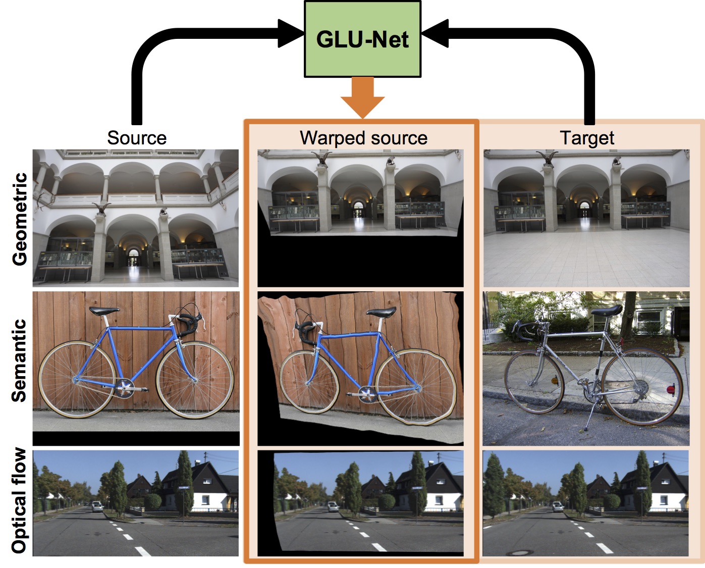
The general problem of estimating correspondences between pairs of images can be divided into several different tasks, depending on the origin of the images. In the geometric matching task [18], the images constitute different views of the same scene, taken by a single or multiple cameras. The images may be taken from radically different viewpoints, leading to large displacements and appearance transformations between the frames. On the other hand, optical flow [4, 20] aims to estimate accurate pixel-wise displacements between two consecutive frames of a sequence or video. In the semantic matching problem [17, 38] (also referred as semantic flow), the task is instead to find semantically meaningful correspondences between different instances of the same scene category or object, such as ‘car’ or ‘horse’. Current methods generally address one of these tasks, using specialized architectures that generalize poorly to related correspondence problems. In this work, we therefore set out to design a universal architecture that jointly addresses all aforementioned tasks.

One key architectural aspect shared by a variety of correspondence networks is the reliance on correlation layers, computing local similarities between deep features extracted from the two images. These provide strong cues when establishing correspondences. Optical flow methods typically employ local correlation layers [13, 23, 24, 26, 57, 58], evaluating similarities in a local neighborhood around an image coordinate. While suitable for small displacements, they are unable to capture large viewpoints changes. On the contrary, geometric and semantic matching architectures utilize global correlations [33, 41, 47, 48, 49], where similarities are evaluated between all pairs of locations in the dense feature maps. While capable of handling long-range matches, global correlation layers are computationally unfeasible at high resolutions. Moreover, they constrain the input image size to a pre-determined resolution, which severely hampers accuracy for high-resolution images.

Contributions: In this paper, we propose GLU-Net, a Global-Local Universal Network for estimating dense correspondences. Our architecture is robust to large viewpoint changes and appearance transformations, while capable of estimating small displacements with high accuracy. The main contributions of this work are: (i) We introduce a single unified architecture, applicable to geometric matching, semantic matching and optical flow. (ii) Our network carefully integrates global and local correlation layers to handle both large and small displacements. (iii) To circumvent the fixed input resolution imposed by the global cost volume, we propose an adaptive resolution strategy that enables our network to take any image resolution as input, crucial for high-accuracy displacements. (iv) We train our network in a self-supervised manner, relying on synthetic warps of real images, thus requiring no annotated ground-truth flow.

We perform comprehensive experiments on the three aforementioned tasks, providing detailed analysis of our approach and thorough comparisons with recent state-of-the-art. Our approach outperforms previous methods for dense geometric correspondences on the HPatches [5] and ETH3D [53] datasets, while setting a new state-of-the-art for semantic correspondences on the TSS [60] dataset. Moreover, our network, without any retraining or fine-tuning, generalizes to optical flow by providing highly competitive results on the KITTI [15] dataset. Both training code and models are available at [61].

2 Related work

Finding correspondences between a pair of images is a classical computer vision problem, uniting optical flow, geometric correspondences and semantic matching. This problem dates back several decades [20], with most classical techniques relying on hand crafted [2, 3, 6, 19, 37, 39, 50] or trained [12, 44, 62] feature detectors/descriptors, or variational formulations [4, 20, 38]. In recent years, CNNs have revolutionised most areas within vision, including different aspects of the image correspondence problem. Here, we focus on Convolutional Neural Network (CNN)-based methods for generating dense correspondences or flow fields, as these are most related to our work.

Optical Flow: Dosovitskiy et al. [13] constructed the first trainable CNN for optical flow estimation, FlowNet, based on a U-Net denoising autoencoder architecture [63] and trained it on the large synthetic FlyingChairs dataset. Ilg et al. [26] stacked several basic FlowNet models into a large one, called FlowNet2, which performed on par with classical state-of-the-art methods on the Sintel benchmark [7]. Subsequently, Ranjan and Black [46] introduced SpyNet, a compact spatial image pyramid network.

Recent notable contributions to end-to-end trainable optical flow include PWC-Net [57, 58] and LiteFlowNet [23], followed by LiteFlowNet2 [24]. They employ multiple constrained correlation layers operating on a feature pyramid, where the features at each level are warped by the current flow estimate, yielding more compact and effective networks. Nevertheless, while these networks excel at small to medium displacements with small appearance changes, they perform poorly on strong geometric transformations or when the visual appearance is significantly different.

Geometric Correspondence: Unlike optical flow, geometric correspondence estimation focuses on large geometric displacements, which can cause significant appearance distortions between the frames. Motivated by recent advancements in optical flow architectures, Melekhov et al. [41] introduced DGC-Net, a coarse-to-fine CNN-based framework that generates dense 2D correspondences between image pairs. It relies on a global cost volume constructed at the coarsest resolution. However, the input size is constrained to a fixed resolution ($240\times 240$), severely limiting its performance on higher resolution images. Rocco et al. [49] aim at increasing the performance of the global correlation layer by proposing an end-to-end trainable neighborhood consensus network, NC-Net, to filter out ambiguous matches and keep only the locally and cyclically consistent ones. Furthermore, Laskar et al. [36] utilize a modified version of DGC-Net, focusing on image retrieval.

Semantic Correspondence: Unlike optical flow or geometric matching, semantic correspondence poses additional challenges due to intra-class appearance and shape variations among different instances from the same object or scene category. Rocco et al. [47, 48] proposed the CNNGeo matching architecture, predicting globally parametrized affine and thin plate spline transformations between image pairs. Other approaches aim to predict richer geometric deformations [10, 31, 32, 49] using e.g. Spatial Transformer Networks [28]. Recently, Jeon et al. [30] introduced PARN, a pyramidal model where dense affine transformation fields are progressively estimated in a coarse-to-fine manner. SAM-Net [33] obtains better results by jointly learning semantic correspondence and attribute transfer. Huang et al. [22] proposed DCCNet, which fuses correlation maps derived from local features and a context-aware semantic feature representation.

3 Method

We address the problem of finding pixel-wise correspondences between a pair of images $I_{\text{s}}\in\mathbb{R}^{H\times W\times 3}$ and $I_{\text{t}}\in\mathbb{R}^{H\times W\times 3}$. In this work, we put no particular assumptions on the origin of the image pair itself. It may correspond to two different views of the same scene, two consecutive frames in a video, or two images with similar semantic content. Our goal is to estimate a dense displacement field, often referred to as flow, $\mathbf{w}\in\mathbb{R}^{H\times W\times 2}$ that warps image $I_{\text{s}}$ towards $I_{\text{t}}$ such that,

$$I_{\text{t}}(\mathbf{x})\approx I_{\text{s}}(\mathbf{x}+\mathbf{w}(\mathbf{x}))\,.$$ (1)

The flow $\mathbf{w}$ represents the pixel-wise 2D motion vectors in the target image coordinate system. It is directly related to the pixel correspondence map $\mathbf{m}(\mathbf{x})=\mathbf{x}+\mathbf{w}(\mathbf{x})$, which directly maps an image coordinate $\mathbf{x}$ in the target image to its corresponding position in the source image.

In this work, we design an architecture capable of robustly finding both long-range correspondences and accurate estimation of pixel-wise displacements. We thereby achieve a universal network for predicting dense flow fields, applicable to geometric matching, semantic correspondences and optical flow. The overall architecture follows a CNN feature-based coarse-to-fine strategy, which has proved widely successful for specific tasks [23, 30, 33, 41, 57]. However, contrary to previous works, our architecture combines global and local correlation layers, as discussed in Section 3.1 and 3.2, to benefit from their complementary properties. We further circumvent the input resolution restriction imposed by the global correlation layer by introducing an adaptive resolution strategy in Section 3.3. It is based on a two-stream feature pyramid, which allows dense correspondence prediction for any input resolution image. Our final architecture is detailed in Section 3.4 and the training procedure explained in Section 3.5.

(a) Local-Net                        (b) Global-Net                        (c) GLOCAL-Net                        (d) GLU-Net (Ours)

Figure 2: Schematic representation of different architectures for dense flow field estimation $\mathbf{w}$. Local-Net (a) and Global-Net (b) employ only local and global correlation layers, respectively. Our GLOCAL-Net (c) combines both to effectively handle short and long-range displacements. GLU-Net (d) additionally employs our adaptive resolution strategy, thus capable of processing high-resolution images.

3.1 Local and Global Correlations

Current state-of-the-art architectures [22, 23, 30, 41, 57] for estimating image correspondences or optical flow rely on measuring local similarities between the source and target images. This is performed in a deep feature space, which provides a discriminative embedding with desirable invariances. The result, generally referred to as a correlation or cost volume, provides an extremely powerful cue when deriving the final correspondence or flow estimate. The correlation can be performed in a local or global manner.

Local correlation: In a local correlation layer, the feature similarity is only evaluated in the neighborhood of the target image coordinate, specified by a search radius $R$. Formally, the correlation $c^{l}$ between the target $F_{\text{t}}^{l}\in\mathbb{R}^{H_{l}\times W_{l}\times d_{l}}$ and source $F_{\text{s}}^{l}\in\mathbb{R}^{H_{l}\times W_{l}\times d_{l}}$ feature maps is defined as,

$$c^{l}(\mathbf{x},\mathbf{d})=F_{\text{t}}^{l}(\mathbf{x})^{T}F_{\text{s}}^{l}(\mathbf{x}+\mathbf{d})\,,\quad\|\mathbf{d}\|_{\infty}\leq R\,,$$ (2)

where $\mathbf{x}\in\mathbb{Z}^{2}$ is a coordinate in the target feature map and $\mathbf{d}\in\mathbb{Z}^{2}$ is the displacement from this location. The displacement is constrained to $\|\mathbf{d}\|_{\infty}\leq R$, i.e. the maximum motion in any direction is $R$. We let $l$ denote the level in the feature pyramid. While most naturally thought of as a 4-dimensional tensor, the two displacement dimensions are usually vectorized into one to simplify further processing in the CNN. The resulting 3D correlation volume $c^{l}$ thus has a dimensionality of $H_{l}\times W_{l}\times(2R+1)^{2}$.

Global correlation: A global correlation layer evaluates the pairwise similarities between all locations in the target and source feature maps. The correlation volume $C^{l}\in\mathbb{R}^{H_{l}\times W_{l}\times H_{l}\times W_{l}}$ contains at each target image location $\mathbf{x}\in\mathbb{Z}^{2}$ the scalar products between corresponding feature vector $F^{l}_{\text{t}}(\mathbf{x})$ and the vectors $F^{l}_{\text{s}}(\mathbf{x^{\prime}})\in\mathbb{R}^{d}$ extracted from all source feature map coordinates $\mathbf{x^{\prime}}$,

$$C^{l}(\mathbf{x},\mathbf{x^{\prime}})=F^{l}_{\text{t}}(\mathbf{x})^{T}F^{l}_{\text{s}}\left(\mathbf{x^{\prime}}\right)\,.$$ (3)

As for the local cost volume, we vectorize the source dimensions, leading to a 3D tensor of size $H_{l}\times W_{l}\times(H_{l}W_{l})$.

Comparison: Local and global correlation layers have a few key contrary properties and behaviors. Local correlations are popularly employed in architectures designed for optical flow [13, 23, 57], where the displacements are generally small. Thanks to their restricted search region, local correlation layers can be applied for high-resolution feature maps, which allows accurate estimation of small displacements. On the other hand, a local correlation based architecture is limited to a certain maximum range of displacements. Conversely, a global correlation based architecture does not suffer from this limitation, encapsulating arbitrary long-range displacements.

The major disadvantage of the global cost volume is that its dimensionality scales with the size of the feature map $H_{l}\times W_{l}$. Therefore, due to the quadratic $\mathcal{O}((H_{l}W_{l})^{2})$ scaling in computation and memory, global cost volumes are only suitable at coarse resolutions. Moreover, post-processing layers implemented with 2D convolutions expect a fixed channel dimensionality. Since the channel dimension $H_{l}W_{l}$ of the cost volume depends on its spatial dimensions $H_{l}\times W_{l}$, this effectively constrains the network input resolution to a fixed pre-determined value, referred to as $H_{L}\times W_{L}$. The network can thus not leverage the more detailed structure in high-resolution images and lacks precision, since the images require down-scaling to $H_{L}\times W_{L}$ before being processed by the network. Architectures with only local correlations (Local-Net) or with a unique global correlation (Global-Net) are visualized in Figure 2a, b.

3.2 Global-Local Architecture

We introduce a unified network that leverages the advantages of both global and local correlation layers and which also circumvents the limitations of both. Our goal is to handle any kind of geometric transformations - including large displacements - while achieving high precision for detailed and small displacements. This is performed by carefully integrating global and local correlation layers in a feature pyramid based network architecture.

Inspired by DGC-Net [41], we employ a global correlation layer at the coarsest level. The purpose of this layer is to handle the long-range correspondences. Since these are best captured in the coarsest scale, only a single global correlation is needed. In subsequent layers, the dense flow field is refined by computing image feature similarity using local correlations. This allows precise estimation of the displacements. Combining global and local correlation layers allows us to achieve robust and accurate prediction of both long and small-range motions. Such an architecture is visualized with GLOCAL-Net in Figure 2c. However, this network is still restricted to a certain input resolution. Next, we introduce a design strategy that circumvents this issue.

3.3 Adaptive resolution

As previously discussed, the global correlation layer imposes a pre-determined input resolution for the network to ensure a constant channel dimensionality of the global cost volume. This severely limits the applicability and accuracy of the correspondence network, since higher resolution images requires down-scaling before being processed by the network, followed by up-scaling of the resulting flow. In this section, we address this key issue by introducing an architecture capable of taking images of any resolution, while still benefiting from a global correlation.

Our adaptive-resolution architecture consists of two sub-networks, which operate on two different image resolutions. The first, termed L-Net, takes source and target images downscaled to a fixed resolution $H_{L}\times W_{L}$, which allows a global correlation layer to be integrated. The H-Net on the other hand, operates directly on the original image resolution $H\times W$, which is not constrained to any specific value. It refines the flow estimate generated by the L-Net with local correlations applied to a shallow feature pyramid constructed directly from the original images. It is schematically represented in Figure 2d.

Both sub-networks are based on a coarse-to-fine architecture, employing the same feature extractor backbone. In detail, the L-Net relies on a global correlation at the coarsest level in order to effectively handle any kind of geometric transformations, including very large displacements. Subsequent levels of L-Net employ local correlations to refine the flow field. It is then up-sampled to the coarsest resolution of H-Net, where it serves as the initial flow estimate used for warping the source features $F_{\text{s}}$. Subsequently, the flow prediction is refined numerous times within H-Net, that operates on the full scale images, thus providing a very detailed, sub-pixel accurate final estimation of the dense flow field relating $I_{\text{s}}$ and $I_{\text{t}}$.

For high-resolution images, the upscaling factor between the finest pyramid level, $l_{L}$, of L-Net and the coarsest, $l_{H}$, of H-Net (see Figure 2d) can be significant. Our adaptive resolution strategy allows additional refinement steps of the flow estimate between those two levels during inference, thus improving the accuracy of the estimated flow, without training any additional weights. This is performed by recursively applying the $l_{H}$ layer weights at intermediate resolutions obtained by down-sampling the source and target features from $l_{H}$. In summary, our adaptive resolution network is capable of seamlessly predicting an accurate flow field in the original input resolution, while also benefiting from robustness to long-range correspondences provided by the global layer. The entire network is trained end-to-end.

Figure 3: Architectural details of our GLU-Net. It is composed of two modules, operating on two different image resolutions. The L-Net (right) relies on a global correlation for long-range matches, while the H-Net (left) refines the flow estimate with local correlations.

3.4 Architecture details

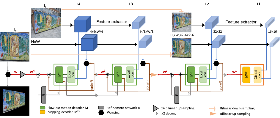
In this section, we provide a detailed description of our architecture. While any feature extractor backbone can be employed, we use the VGG-16 [8] network trained on ImageNet [35] to provide a fair comparison to previous works in geometric [41] and semantic correspondences [30]. For our L-Net, we set the input resolution to $(H_{L}\times W_{L})=(256\times 256)$. It is composed of two pyramid levels, using Conv5-3 ($16\times 16$ resolution) and Conv4-3 ($32\times 32$ resolution) respectively. The former employs global correlation, while the latter is based on a local correlation. The H-Net is composed of two feature pyramid levels extracted from the original image resolution $H\times W$. For this purpose, we employ Conv4-3 and Conv3-3 having resolutions $\frac{H}{8}\times\frac{W}{8}$ and $\frac{H}{4}\times\frac{W}{4}$ respectively. The H-Net is purely based on local correlation layers. Our final architecture GLU-Net, composed of four pyramid levels in total, is detailed in Figure 3. Next, we describe the various architectural components.

Coarsest resolution and mapping estimation: We compute a global correlation from the $L^{2}$-normalized source and target features. The cost volume is further post-processed by applying channel-wise $L^{2}$-normalisation followed by ReLU [42] to strongly down-weight ambiguous matches [47]. Similar to DGC-Net [41], the resulting global correlation C is then fed into a correspondence map decoder $M_{\text{top}}$ to estimate a 2D dense correspondence map $\mathbf{m}$ at the coarsest level $L1$ of the feature pyramid:

$$\mathbf{m}^{1}=M_{\text{top}}\left(C\left(F_{\text{t}}^{1},F_{\text{s}}^{1}\right)\right)\,.$$ (4)

The correspondence map is then converted to a displacement field, as $\mathbf{w}^{1}(\mathbf{x})=\mathbf{m}^{1}(\mathbf{x})-\mathbf{x}$.

Subsequent flow estimations: The flow is refined by local correlation modules. At level $l$, the flow decoder $M$ infers the residual flow $\Delta\mathbf{\tilde{w}}^{l}$ as,

$$\Delta\mathbf{\tilde{w}}^{l}=M\left(c\left(F_{\text{t}}^{l},\widetilde{F}_{\text{s}}^{l};R\right),\operatorname{up}\!\left(\mathbf{w}^{l-1}\right)\right)\,.$$ (5)

$c$ is a local correlation (2) with search radius $R$ and $\widetilde{F}_{\text{s}}^{l}(\mathbf{x})=F_{\text{s}}^{l}\left(\mathbf{x}+\operatorname{up}\left(\mathbf{w}^{l-1}\right)(\mathbf{x})\right)$ is the warped source feature map $F_{\text{s}}$ according to the upsampled flow $\operatorname{up}\!\left(\mathbf{w}^{l-1}\right)$. The complete flow field is computed as $\mathbf{\tilde{w}}^{l}=\Delta\mathbf{\tilde{w}}^{l}+\operatorname{up}\!\left(\mathbf{w}^{l-1}\right)$.

Flow refinement: Contextual information have been shown advantageous for pixel-wise prediction tasks [9, 22]. We thus use a sub-network R, called the refinement network, to post-process the estimated flow at the highest levels of L-Net and H-Net (L2 and L4 in Figure 3) by effectively enlarging the receptive field size. It takes the features $f^{l}$ of the second last layer from the flow decoder $M^{l}$ as input and outputs the refined flow $\mathbf{w}^{l}=R\left(f^{l}\right)+\mathbf{\tilde{w}}^{l}$. For the other pyramid level (L3), the final flow field is $\mathbf{w}^{l}=\mathbf{\tilde{w}}^{l}$.

Cyclic consistency: Since the quality of the correlation is of primary importance for the flow estimation process, we introduce an additional filtering step on the global cost volume to enforce the reciprocity constraint on matches. We employ the soft mutual nearest neighbor filtering introduced by [49] and apply it to post-process the global correlation.

3.5 Training

Loss: We train our network in a single phase. We freeze the pre-trained backbone feature extractor during training. Following FlowNet [13], we apply supervision at every pyramid level using the endpoint error (EPE) loss with respect to the ground truth displacements.

Dataset: Our network is solely trained on pairs generated by applying random warps to the original images. Since our network is designed to also estimate correspondences between high-resolution images, training data of sufficient resolution is preferred in order to utilize the full potential of our architecture. We use a combination of the DPED [25], CityScapes [11] and ADE-20K [64] datasets, which have images larger than $750\times 750$. On the total dataset of $40,000$ images, we apply the same synthetic transformations as in tokyo (DGC-Net [41] training data). The resulting image pairs are cropped to $520\times 520$ for training. We call this dataset DPED-CityScape-ADE. More training and architectural details are available in the appendix Sections A and B.

Figure 4: Qualitative comparison with state-of-the-art on geometric correspondence datasets. Top: Pairs of HP images. Bottom: Pairs of images from ETH3D taken by two different cameras. Our approach effectively handles large variations in view-point and appearance.

4 Experimental Validation

In this section, we comprehensively evaluate our approach for three diverse problems: geometric matching, semantic correspondences and optical flow. Importantly, we use the same network and model weights, trained on DPED-CityScape-ADE, for all three applications. More detailed results are available in the appendix Section C.

4.1 Geometric matching

We first apply our GLU-Net for the task of geometric matching. The images thus consist of different views of the same scene and include large geometric transformations.

HP: As in DGC-Net [41], we employ the 59 sequences of the HPatches dataset [5] labelled with v_X, which have viewpoint changes, thus excluding the ones labelled i_X, which only have illumination changes. Each image sequence contains a source image and 5 target images taken under increasingly larger viewpoints changes, with sizes ranging from $450\times 600$ to $1613\times 1210$. In addition to evaluating on the original image resolution (referred to as HP), we also evaluate on downscaled ($240\times 240$) images and ground-truths (HP-240) following [41].

ETH3D: To validate our approach for real 3D scenes, where image transformations are not constrained to simple homographies, we also employ the Multi-view dataset ETH3D [53]. It contains 10 image sequences at $480\times 752$ or $514\times 955$ resolution, depicting indoor and outdoor scenes. The authors additionally provide a set of sparse geometrically consistent image correspondences (generated by [51]) that have been optimized over the entire image sequence using the reprojection error. We sample image pairs from each sequence at different intervals to analyze varying magnitude of geometric transformations, and use the provided points as sparse ground truth correspondences. This results in about 500 image pairs in total for each selected interval.

Metrics: In line with [41], we employ the Average End-Point Error (AEPE) and Percentage of Correct Keypoints (PCK) as the evaluation metrics. AEPE is defined as the Euclidean distance between estimated and ground truth flow fields, averaged over all valid pixels of the target image. PCK is computed as the percentage of correspondences $\mathbf{\tilde{x}}_{j}$ with an Euclidean distance error $\left\|\mathbf{\tilde{x}}_{j}-\mathbf{x}_{j}\right\|\leq\delta$, w.r.t. to the ground truth $\mathbf{x}_{j}$, that is smaller than a threshold $\delta$.

Compared methods: We compare with DGC-Net [41] trained on tokyo, which is the current state-of-the-art for dense geometric matching. For a fair comparison we also train a version, called DGC-Net^†, using the same data (DPED-CityScape-ADE) as our GLU-Net. We additionally compare with two state-of-the-art optical flow methods, PWC-Net [57] and LiteFlowNet [23], both trained on Flying-Chairs [13] followed by 3D-things [26]. We use the PyTorch [45] implementations [41, 43, 57] of the models and the pre-trained weights provided by the authors.

	HP-240x240				HP
	Run-time	AEPE	PCK-1px	PCK-5px	AEPE	PCK-1px	PCK-5px
LiteFlowNet [23]	45.10 ms	19.41	28.36 %	57.66 %	118.85	13.91 %	31.64 %
PWC-Net [57, 58]	38.51 ms	21.68	20.99 %	54.19 %	96.14	13.14 %	37.14 %
DGC-Net [41]	138.30 ms	9.07	50.01 %	77.40 %	33.26	12.00 %	58.06 %
DGC-Net†	138.30 ms	9.12	43.09 %	79.35 %	33.47	9.19 %	56.02 %
GLU-Net (Ours)	38.10 ms	7.40	59.92 %	83.47 %	25.05	39.55 %	78.54 %

Table 1: Comparison of state-of-the-art algorithms applied to the task of geometric matching, on the HPatches dataset [5]. Lower AEPE and higher PCK are better.

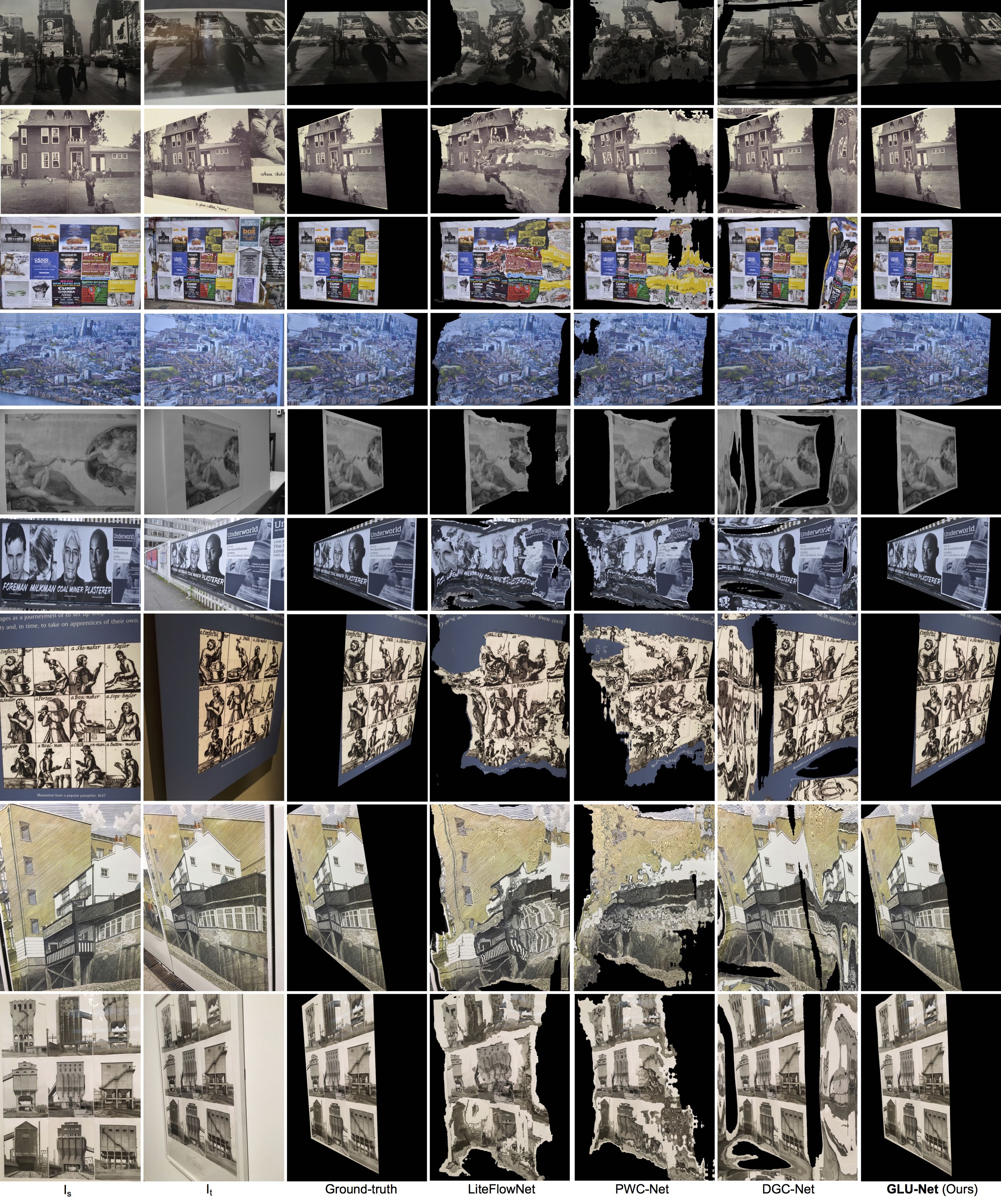
Results: We first present results on the HP and HP-240 in Table 1. Our model strongly outperforms all others by a large margin both in terms of accuracy (PCK) and robustness (AEPE). It is interesting to note that while our model is already better than DGC-Net on the small resolution HP-240, the gap in performance further broadens when increasing the image resolution. Particularly, GLU-Net obtains a PCK-1px value almost four times higher than that of DGC-Net on HP. This demonstrates the benefit of our adaptive resolution strategy, which enables to process high-resolution images with high accuracy. Moreover, our model achieves a 3.6 times faster inference compared to DGC-Net. Figure 4 shows qualitative examples of different networks applied to HP images and ETH3D image pairs taken by two different cameras. Our GLU-Net is robust to large view-points variations as well as drastic changes in illumination.

Figure 5: Quantitative results on geometric matching dataset ETH3D [53]. AEPE and PCK-5 are computed on pairs of images sampled from consecutive images of ETH3D at different intervals.

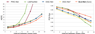
In Figure 5, we plot AEPE and PCK-5px obtained on the ETH3D scenes for different intervals between image pairs. For small intervals, finding correspondences strongly resembles optical flow task while increasing it leads to larger displacements. Therefore, specialised optical flow methods PWC-Net [57] and LiteFlowNet [23] obtain slightly better AEPE and PCK for low intervals, but rapidly degrade for larger ones. In all cases, our approach consistently outperforms DGC-Net [41] in both metrics by a large margin.

4.2 Semantic matching

Here, we perform experiments for the task of semantic matching, where images depict different instances of the same object category, such as cars or horses. We use the same model and weights as in the previous section.

Dataset and metric: We use the TSS dataset [60], which provides dense flow fields annotations for the foreground object in each pair. It contains 400 image pairs, divided into three groups: FG3DCAR, JODS, and PASCAL, according to the origins of the images. Following Taniai et al. [60], we report the PCK with a distance threshold equal to $\alpha\cdot\max(H_{s},W_{s})$, where $H_{s}$ and $W_{s}$ are the dimensions of the source image and $\alpha=0.05$.

Compared methods: We compare to several recent state-of-the-art methods specialised in semantic matching [22, 30, 31, 33, 48, 49]. In addition to our universal network, we evaluate a version that adopts two architectural details that are used in the semantic correspondence literature. Specifically, we add a consensus network [49] for the global correlation layer and concatenate features from different levels in the L-Net, similarly to [30] (see Section 4.4 for an analysis). We call this version Semantic-GLU-Net. To accommodate reflections, which do not occur in geometric correspondence scenarios, we infer the flow field on original and flipped versions of the target image and output the flow field with least horizontal average magnitude.

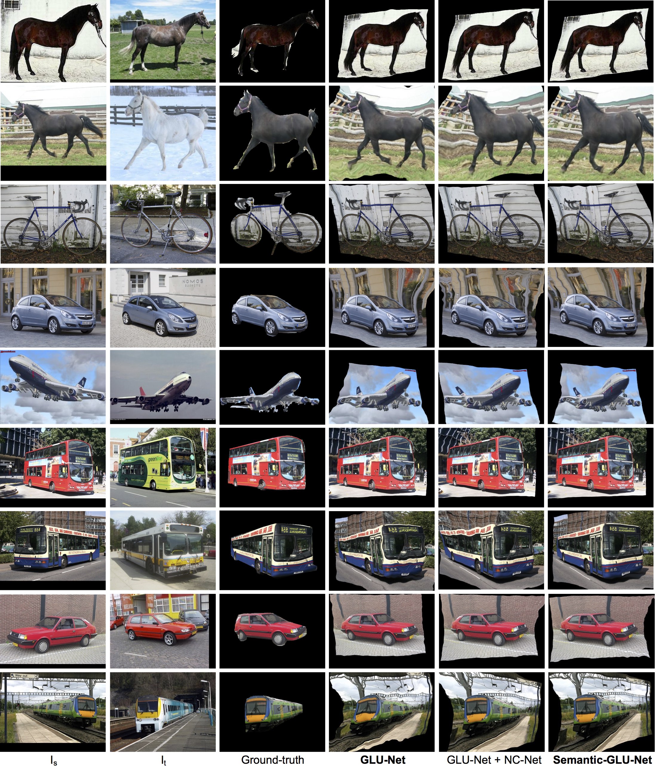
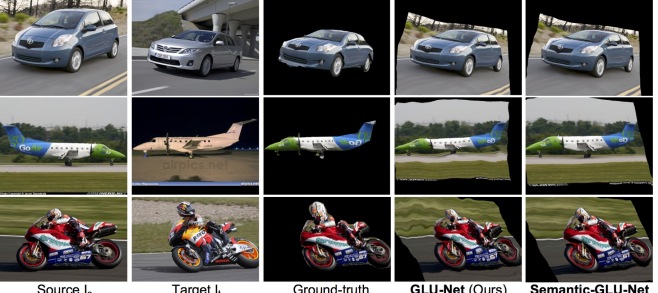
Results: We report results on TSS in Table 2. Our universal network obtains state-of-the-art performance on average over the three TSS groups. Moreover, individual results on FG3Dcar and PASCAL are very close to best metrics. This shows the generalization properties of our network, which is not trained on the same magnitude of semantic data. In contrast, most specialized approaches fine-tuned on PASCAL data [17]. Finally, including architectural details specifically for semantic matching, termed Semantic-GLU-Net, further improves our performance, setting a new state-of-the-art on TSS, by improving a substantial $1.0\%$ PCK over the previous best. Interestingly, we outperform methods that use a deeper, more powerful feature backbone. Qualitative examples of our approach are shown in Figure 6.

Methods	Feature backbone	FG3DCar	JODS	PASCAL	Avg.
CNNGeo(W) [48]	ResNet-101	90.3	76.4	56.5	74.4
RTNs [31]	ResNet-101	90.1	78.2	63.3	77.2
PARN [30]	VGG-16	87.6	71.6	68.8	76.0
PARN [30]	ResNet-101	89.5	75.9	71.2	78.8
NC-Net [49]	ResNet-101	94.5	81.4	57.1	77.7
DCCNet [22]	ResNet-101	93.5	82.6	57.6	77.9
SAM-Net [33]	VGG-19	96.1	82.2	67.2	81.8
GLU-Net	VGG-16	93.2	73.3	71.1	79.2
Semantic-GLU-Net	VGG-16	94.4	75.5	78.3	82.8

Table 2: PCK [%] obtained by different state-of-the-art methods on TSS [60] for the task of semantic matching.

Figure 6: Qualitative examples of GLU-Net (Ours) and Semantic-GLU-Net applied to TSS images [60].

4.3 Optical flow

Finally, we apply our network, with the same weights as previously, for the task of optical flow estimation. Here, the image pairs stem from consecutive frames of a video.

Dataset and metric: For optical flow evaluation, we use the KITTI dataset [15], which is composed of real road sequences captured by a car-mounted stereo camera rig. The 2012 set only consists of static scenes while the 2015 set is extended to dynamic scenes. For this task, we follow the standard evaluation metric, namely the Average End-Point Error (AEPE). We also use the KITTI-specific F1 metric, which represents the percentage of outliers.

Compared methods: We employ state-of-the-art PWC-Net [57, 58] and LiteFlowNet [23] trained on Flying-Chairs [13] and 3D-things [26]. We also compare to DGC-Net [41] (tokyo) and DGC-Net^† (DPED-CityScape-ADE).

	KITTI-2012		KITTI-2015
	AEPE-all	F1-all [%]	AEPE-all	F1-all [%]
LiteFlowNet [23]	4.00	17.47∗	10.39	28.50
PWC-Net [57, 58]	4.14	20.28∗	10.35	33.67
DGC-Net [41]	8.50∗	32.28∗	14.97∗	50.98∗
DGC-Net†	7.96	34.35	14.33	50.35
GLU-Net	3.34	18.93	9.79	37.52

Table 3: Quantitative results on optical flow KITTI training datasets [15]. Fl-all: Percentage of outliers averaged over all pixels. Inliers are defined as $AEPE<3$ pixels or $<5\%$. Lower F1 and AEPE are best. ^∗ Denotes values which are computed using the trained models provided by the authors.

Results: Since we do not finetune our model, we only evaluate on the KITTI training sets. For fair comparison, we compare to models not finetuned on the KITTI training data. The results are shown in Table 3 and a qualitative example is illustrated in Figure 7. Our network obtains highest AEPE on both KITTI-2012 and 2015. Nevertheless, we observe that our method achieves a larger F1 on KITTI-2015 compared to approaches specifically trained and designed for optical flow. This is largely due to our self-supervised training data, which currently does not model independently moving objects or occlusions, but could be included to pursue a more purposed optical flow solution. Yet, our approach demonstrates competitive results for this challenging task, without training on any optical flow data. This clearly shows that our network can not only robustly estimate long-range matches, but also accurate small displacements.

Figure 7: Visualization of the flow outputted by different methods for a KITTI-2012 image.

4.4 Ablation study

Here, we perform a detailed analysis of our approach.

Local-global architecture: We first analyze the impact of global and local correlation layers in our dense correspondence framework. We compare using only local layers (Local-Net), a global layer (Global-Net) and our combination (GLOCAL-Net), presented in Figure 2. As shown in Table 4, Local-Net fails on the HP dataset, due to its inability to capture large displacements. While the Global-Net can handle large viewpoint changes, it achieves inferior accuracy compared to GLOCAL-Net, which additionaly integrates local correlations layers.

Adaptive resolution: By further adding the adaptive resolution strategy (Section 3.3), our approach (GLU-Net in Table 4) achieves a large performance gain in all metrics compared to GLOCAL-Net. This improvement is most prominent for high resolution images, i.e. the original HP data.

Iterative refinement: From Table 4, applying iterative refinement (it-R) clearly benefits accuracy for high-resolution images (HP). This further allows us to seamlessly add extra flow refinements, without incurring any additional network weights, in order to process images of high resolution.

Global correlation: Lastly, we explore design choices for the global correlation block in our architecture. As shown in Table 5, adding cyclic consistency (CC) [49] as a post-processing brings improvements for all datasets. Subsequently adding NC-Net and concatenating features of L-Net (Concat-F) lead to major overall gain on the HP [5] and TSS [60] datasets. However, we observe a slight degradation in accuracy, as seen on KITTI [15]. We therefore only include these components for the Semantic-GLU-Net version (Section 4.2) and not in our universal GLU-Net.

		Local-	Global-	GLOCAL-	GLU-Net	GLU-Net
		Net	Net	Net	(no CC, no it-R)	(no CC, it-R)
HP-240	AEPE	10.62	9.72	8.77	7.69	7.69
	PCK-1px [%]	35.10	41.28	48.53	53.83	53.83
	PCK-5px [%]	73.03	72.76	78.12	83.17	83.17
HP	AEPE	147.96	34.64	31.64	25.55	25.09
	PCK-1px [%]	7.41	8.86	10.23	35.26	36.81
	PCK-5px [%]	19.27	50.11	56.73	75.79	77.55

Table 4: Effect of global and local correlations as well of adaptive resolution strategy. it-R: iterative refinement, introduced with our adaptive resolution (Section 3.3), CC: cyclic-consistency [49].

		No CC	+ CC (Ours)	+ NC-Net	+ Concat-F
HP	AEPE	25.09	25.05	22.00	21.40
	PCK-1px [%]	36.81	39.55	37.62	38.49
	PCK-5px [%]	77.55	78.54	79.41	79.50
KITTI-	AEPE	3.56	3.34	3.80	3.85
2012	F1-all [%]	21.67	18.93	23.49	23.84
TSS	PCK [%]	78.97	79.21	82.10	82.76

Table 5: Effect of additional architectural details. All models are with iterative refinement. We add CC: cyclic-consistency [49], NC-Net: Neighborhood Consensus network [49], Concat-F: Concatenation of features of L-Net [30].

5 Conclusion

We propose a universal coarse-to-fine architecture for estimating dense flow fields from a pair of images. By carefully combining global and local correlation layers, our network effectively estimates long-range displacements while also achieving high accuracy. Crucially, we introduce an adaptive resolution strategy to counter the fixed input resolution otherwise imposed by the global correlation. Our universal GLU-Net is thoroughly evaluated for the three diverse tasks of geometric correspondences, semantic matching and optical flow. When using the same model weights, our network achieves state-of-the-art performance on all above tasks, demonstrating its universal applicability.

Acknowledgments: This work was partly supported by the ETH Zürich Fund (OK), a Huawei Technologies Oy (Finland) project, an Amazon AWS grant, and Nvidia.

Appendix

In this supplementary material, we first provide details about the architecture of the different modules of our network GLU-Net in Section A. We then explain the training procedure in more depth in Section B. Finally, we present additional qualitative results and more detailed quantitative experiments in Section C.

Appendix A Architecture details

In this section, we provide additional details about cyclic consistency as a post processing step of the global correlation. We also give a detailed architectural description of the mapping and flow decoders, along with the refinement network. Lastly, we explain in depth the iterative refinement allowed by our adaptive resolution strategy. In the following, a convolution layer or block refers to the composition of a 2D-convolution followed by batch norm [27] and ReLU [42] (Conv-BN-ReLU).

A.1 Cyclic consistency post-processing step for improved global correlation

Since the quality of the correlation layer output is of primary importance for the flow estimation process, we introduce an additional filtering step on the global cost volume to enforce the reciprocity constraint on matches. To encourage matched features to be mutual nearest neighbours, we employ the soft mutual nearest neighbor filtering introduced by [49] and apply it to post-process the global correlation.

The soft mutual nearest neighbor module filters a global correlation $C\in\mathbb{R}^{H\times W\times H\times W}$ into $\hat{C}\in\mathbb{R}^{H\times W\times H\times W}$ such that:

$$\hat{C}(i,j,k,l)=r_{t}(i,j,k,l)\cdot r_{s}(i,j,k,l)\cdot C(i,j,k,l)$$ (6)

with $r_{s}(i,j,k,l)$ and $r_{t}(i,j,k,l)$ the ratios of the score of the particular match $C(i,j,k,l)$ with the best scores along each pair of dimensions corresponding to images $I_{\text{s}}$ and $I_{\text{t}}$ respectively. We present the formula for $r_{s}(i,j,k,l)$ below, the same applies for $r_{t}(i,j,k,l)$.

$$r_{t}(i,j,k,l)=\frac{C(i,j,k,l)}{\max_{ab}C(a,b,k,l)}$$ (7)

This cyclic consistency post-processing step does not add any training weights.

A.2 Mapping decoder $M_{\text{top}}$

In this sub-section, we give additional details of the mapping decoder $M_{\text{top}}$ for the global correlation layer (Eq. 4 and Figure 3 in the paper). We compute a global correlation from the $L^{2}$-normalized source and target features. The cost volume is further post-processed by applying channel-wise $L^{2}$-normalisation followed by ReLU [42] to strongly down-weight ambiguous matches [47]. Similar to DGC-Net [41], the resulting global correlation layer C is then fed into a correspondence map decoder $M_{\text{top}}$ to estimate a 2D dense correspondence map $\mathbf{m}$ at the coarsest level $L_{1}$ of the feature pyramid,

$$\mathbf{m}^{1}=M_{\text{top}}\left(C\left(\frac{F_{\text{t}}^{1}}{\left\|F_{\text{t}}^{1}\right\|},\frac{F_{\text{s}}^{1}}{\left\|F_{\text{s}}^{1}\right\|}\right)\right)\,.$$ (8)

The outputted mapping estimate is parameterized such that each predicted pixel location in the map belongs to the interval $\left[-1;1\right]$ representing width and height normalized image coordinates. The correspondence map is then re-scaled to image coordinates and converted to a displacement field.

$$\mathbf{w}^{1}(\mathbf{x})=\mathbf{m}^{1}(\mathbf{x})-\mathbf{x}\,.$$ (9)

The decoder $M_{top}$ consists of 5 feed-forward convolutional blocks with a $3\times 3$ spatial kernel. The number of feature channels of each convolutional layers are respectively 128, 128, 96, 64, and 32. The final output of the mapping decoder is the result of a linear 2D convolution, without any activation.

A.3 Flow decoder $M$

Here, we give additional details of the flow decoder $M$ for the local correlation layers (Eq. 5 and Figure 3 in the paper). At level $l$, the flow decoder $M$ infers the residual flow $\Delta\mathbf{\tilde{w}}^{l}$ as,

$$\Delta\mathbf{\tilde{w}}^{l}=M\left(c\left(F_{\text{t}}^{l},\widetilde{F}_{\text{s}}^{l};R\right),\operatorname{up}(\mathbf{w}^{l-1})\right)\,.$$ (10)

Here, $c$ is a local correlation volume with search radius $R$ and $\widetilde{F}_{\text{s}}^{l}(\mathbf{x})=F_{\text{s}}^{l}\left(\mathbf{x}+\operatorname{up}\left(\mathbf{w}^{l-1}\right)(\mathbf{x})\right)$ is the warped source feature map $F_{\text{s}}$ according to the upsampled flow from the previous pyramid level $\operatorname{up}\left(\mathbf{w}^{l-1}\right)$. The complete flow field is then computed as $\mathbf{\tilde{w}}^{l}=\Delta\mathbf{\tilde{w}}^{l}+\operatorname{up}\left(\mathbf{w}^{l-1}\right)$.

The flow decoder at level 4 (see Figure 3 of main paper) additionally takes an input $\operatorname{de}_{2}(f^{l-1})$, obtained by applying a transposed convolution layer $\operatorname{de}_{2}$ to the features $f^{l-1}$ of the second last layer from the flow decoder $M^{l-1}$. This additional inputs was first introduced and utilized in PWC-Net [57] at every pyramid level. It enables the decoder of the current level to obtain some information about the correlation at the previous level. In GLU-Net, this additional input to the flow decoder only appears in H-Net since in L-Net, a global correlation and mapping decoder precede the flow decoder.

As for the flow decoder $M$, we employ a similar architecture to the one in PWC-Net [57]. It consists of 5 convolutional layers with DenseNet connections [21]. The numbers of feature channels at each convolutional layers are respectively 128, 128, 96, 64, and 32, and the spatial kernel of each convolution is $3\times 3$. DenseNet connections are used since they have been shown to lead to significant improvement in image classification [21] and optical flow estimation [57]. The final output of the flow decoder is the result of a linear 2D convolution, without any activation.

A.4 Refinement network $R$

Here, we explain in more details the refinement network R (Figure 3 in the paper). The refinement network aims to refine the pixel-level flow field $\mathbf{\tilde{w}}^{l}$, thus preventing erroneous flows from being amplified by up-sampling and passing to the next pyramid level. Its architecture is the same than the context network employed in PWC-Net [57]. It is a feed-forward CNN with 7 dilated convolutional layers [56], with varying dilation rates. Dilated convolutions enlarge the receptive field without increasing the number of weights. From bottom to top, the dilation constants are 1, 2, 4, 8, 16, 1, and 1. The spatial kernel is set to $3\times 3$ for all convolutional layers.

A.5 Details about Local-net, Global-Net and GLOCAL-Net

In Figure 2 of the main paper, we introduced Local-Net, Global-Net and GLOCAL-Net to investigate the differences between architectures based on local correlation layers, a global correlation layer or a combination of the two, respectively. All three networks are composed of three pyramid levels and use the same feature extractor backbone VGG-16 [8]. The mapping and flow decoders have the same architecture as those used for GLU-Net and described above. For Global-Net, the pyramid levels following the global correlation level employ concatenation of the target and warped source feature maps, as suggested in DGC-Net [41]. They are fed to the flow estimation decoder along with the up-sampled flow from the previous resolution. Finally, Global-Net and GLOCAL-Net are both restricted to a pre-determined input resolution $H_{L}\times W_{L}$ due to their global correlation at the coarsest pyramid level. On the other hand, Local-Net, which only relies on local correlations, can take input images of any resolutions.

A.6 Iterative refinement

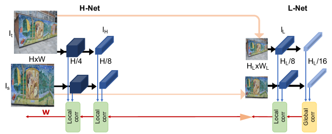
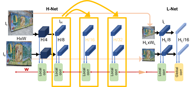
Here we provide more details about the iterative refinement procedure described in 3.3 in the paper. For high-resolution images, the upscaling factor between the finest pyramid level, $l_{L}$, of L-Net and the coarsest, $l_{H}$, of H-Net (see Figure 8) can be significant. Our adaptive resolution strategy allows additional refinement steps of the flow estimate between those two levels during inference, thus improving the accuracy of the estimated flow, without training any additional weights. This is performed by recursively applying the $l_{H}$ layer weights at intermediate resolutions obtained by down-sampling the source and target feature maps from $l_{H}$.

Particularly, we apply iterative refinement if the ratio between the resolutions of the $l_{H}$ and $l_{L}$ levels is larger than three. We then iteratively perform refinements at intermediate resolutions, obtained by a reduction of factor 2 from $l_{H}$ in each step, until the ratio between the resolution of the coarsest intermediate level and the resolution of $l_{L}$ is smaller than 2.

In more details, we construct a local correlation layer from the source and target feature maps of level $l_{H}$ down-sampled to the desired intermediate resolution. We then apply the weights of the level $l_{H}$ decoder to the local correlation, therefore obtaining an intermediate refinement of the flow field. This process is illustrated in Figure 8, where the gap between $l_{L}$ and $l_{H}$ here allows for two additional flow field refinements.

(a) GLU-Net without iterative refinement.

(b) GLU-Net with iterative refinement between L-Net and H-Net.

Figure 8: Schematic representation of iterative refinement. The features and weights of $l_{H}$ level of H-Net are iteratively applied at intermediate resolutions between L-Net and H-Net.

Appendix B Training details

Here, we provide additional details about the training procedure and the training dataset.

B.1 Loss

We freeze the weights of the feature extractor during training. Let $\theta$ denote the learnable parameters of the network. Let $\mathbf{w}_{\theta}^{l}=(\mathbf{w_{x}}^{l},\mathbf{w_{y}}^{l})\in\mathbb{R}^{H_{l}\times W_{l}\times 2}$ denote the flow field estimated by the network at the $l^{th}$ pyramid level. $\mathbf{w}_{\mathrm{GT}}^{l}$ refers to the corresponding dense flow ground-truth, computed from the random warp. We employ the multi-scale training loss, first introduced in FlowNet [13],

$$\mathcal{L}(\theta)=\sum_{l=L_{1}}^{L}\alpha_{l}\sum_{\mathbf{x}}\left\|\mathbf{w}_{\theta}^{l}(\mathbf{x})-\mathbf{w}_{\mathrm{GT}}^{l}(\mathbf{x})\right\|+\gamma\left\|\theta\right\|\,,$$ (11)

where $\alpha_{l}$ are the weights applied to each pyramid level and the second term of the loss regularizes the weights of the network. We do not apply any mask during training, which means that occluded regions (that do not have visible matches) are included in the training loss. Since the image pairs are related by synthetic transformations, these regions do have a correct ground-truth flow value.

For our adaptive resolution strategy, we down-sample and scale the ground truth from original resolution $H\times W$ to $H_{L}\times W_{L}$ in order to obtain the ground truth flow fields for L-Net. Similarly to FlowNet [13] and PWC-Net [57], we down-sample the ground truth from the base resolution to the different pyramid resolutions without further scaling, so as to obtain the supervision signals at the different levels.

B.2 Dataset

To use the full potential of our GLU-Net, training should be performed on high-resolution images. We create the training dataset following the procedure in DGC-Net [41], but enforcing the condition of high resolution. We use the same $40,000$ synthetic transformations (affine, thin-plate and homographies), but apply them to our higher resolution images collected from the DPED [25], CityScapes [11] and ADE-20K [64] datasets. Indeed, DPED images are very large, however the DPED training dataset is composed of only approximately 5000 sets of images taken by four different cameras. We use the images from two cameras, resulting in around $10,000$ images. CityScapes additionally adds about $23,000$ images. We complement with a random sample of ADE-20K images with a minimum resolution of $750\times 750$.

B.3 Implementation details

As a preprocessing step, the training images are mean-centered and normalized using mean and standard deviation of ImageNet dataset [35]. For all local correlation layers, we employ a search radius $R=4$. For the training of Global-Net and GLOCAL-Net, which both have a pre-determined fixed input image resolution of $(H_{L}\times W_{L}=256\times 256)$, we use a batch size of 32 while we train LOCAL-Net, which can take any input image, with batches of size 16. We set the initial learning rate to $10^{-2}$ and gradually decrease it during training. The weights in the training loss are set to be $\alpha_{1}=0.32,\alpha_{2}=0.08,\alpha_{3}=0.02$.

Our final network GLU-Net is trained with a batch size of 16 and the learning rate initially equal to $10^{-4}$. The weights in the training loss are set to be $\alpha_{1}=0.32,\alpha_{2}=0.08,\alpha_{3}=0.02,\alpha_{4}=0.01$. Our system is implemented using Pytorch [45] and our networks are trained using Adam optimizer [34] with learning rate decay of $0.0004$.

	HP-240x240			HP			KITTI-2012		KITTI-2015
	AEPE	PCK-1px [%]	PCK-5px [%]	AEPE	PCK-1px [%]	PCK-5px [%]	AEPE-all	F1-all [%]	AEPE-all	F1-all [%]
DGC-Net (tokyo)	9.07	50.01	77.40	33.26	12.00	58.06	8.50	32.38	14.97	50.98
DGC-Net† (DPED-CityScape-ADE)	9.12	43.09	79.35	33.47	9.19	56.02	7.96	34.35	14.33	50.35
GLU-Net (DPED-CityScape-ADE)	7.40	59.92	83.47	25.05	39.55	78.54	3.34	18.93	9.79	37.52

Table 6: Effect of the training dataset on the evaluation results of DGC-Net and comparison to GLU-Net. The training dataset is indicated in parenthesis.

		HP-240					HP
		I	II	III	IV	V	all	I	II	III	IV	V	all
	AEPE	6.99	16.78	19.13	25.27	28.89	19.41	36.69	102.17	113.58	154.97	186.82	118.85
LiteFlowNet	PCK-1px [%]	50.06	28.93	25.87	23.22	13.72	28.36	34.86	12.95	10.35	6.93	4.47	13.91
	PCK-5px [%]	82.14	59.62	56.92	51.04	38.59	57.66	63.99	32.88	28.99	18.52	13.85	31.64
	AEPE	5.74	17.69	20.46	27.61	36.97	21.68	23.93	76.33	91.30	124.22	164.91	96.14
PWC-Net	PCK-1px [%]	43.55	20.35	18.60	14.17	8.27	20.99	31.56	12.10	10.83	7.09	4.12	13.14
	PCK-5px [%]	80.06	57.08	53.89	45.70	34.22	54.19	68.79	38.51	36.38	25.24	16.76	37.14
	AEPE	1.74	5.88	9.07	12.14	16.50	9.07	5.71	20.48	34.15	43.94	62.01	33.26
DGC-Net	PCK-1px [%]	70.29	53.97	52.06	41.02	32.74	50.01	20.92	12.88	12.85	7.66	5.67	12.00
	PCK-5px [%]	93.70	82.43	77.58	71.53	61.78	77.40	78.88	63.37	60.21	48.83	38.99	58.06
	AEPE	1.90	5.65	9.42	11.39	17.26	9.11	6.04	21.60	32.87	41.82	65.03	33.47
DGC-Net†	PCK-1px [%]	60.88	47.88	46.01	34.87	25.80	43.09	15.81	9.86	9.84	6.17	4.29	9.19
	PCK-5px [%]	93.47	84.04	80.28	74.93	63.76	79.35	75.44	62.16	59.58	46.71	36.21	56.02
	AEPE	0.59	4.05	7.64	9.82	14.89	7.40	1.55	12.66	27.54	32.04	51.47	25.05
GLU-Net (Ours)	PCK-1px [%]	87.89	67.49	62.31	47.76	34.14	59.92	61.72	42.43	40.57	29.47	23.55	39.55
	PCK-5px [%]	99.14	92.39	85.87	78.10	61.84	83.47	96.15	84.35	79.46	73.80	58.92	78.54

Table 7: Details of AEPE and PCK evaluated over each view-point ID of HP and HP-240 datasets.

Figure 9: PCK curves obtained by state-of-the-art methods and GLU-Net over the different view-points of HP.

Appendix C Detailed results

Here, we first provide additional details on the run-time computation in Section C.1. Then, in Section C.2, we evaluate the influence of the training dataset on the evaluation results. We then present additional qualitative and more detailed quantitative results on subsequently the geometric matching, the semantic matching and the optical flow tasks in respectively Sections C.3,  C.4 and C.5. Finally, we expose additional ablation experiments in Section C.6.

C.1 Run time

We compare the run time of our method with state-of-the-art approaches over the HP-240 images in Table 8. The timings have been obtained on the same desktop with an NVIDIA GTX 1080 Ti GPU. The HP-240 images are of size $240\times 240$, which corresponds to the pre-determined input resolution of DGC-Net. For PWC-Net, LiteFlowNet and GLU-Net, the images are resized to $256\times 256$ before being passed through the networks. We do not consider this resizing in the estimated time. They all output a flow at a quarter resolution the input image. We up-scale to the image resolution $240\times 240$ with bilinear interpolation. This up-scaling operation is included in the estimated time.

Our network GLU-Net obtains similar run time than PWC-Net and is three times faster than DGC-Net. This is due to the fact that PWC-Net, LiteFlowNet and GLU-Net outputs a flow at a quarter image resolution whereas DGC-Net refines the estimated flow field with two additional pyramid levels until the fixed resolution of $240\times 240$.

	PWC-Net	LiteFlowNet	DGC-Net	GLU-Net (Ours)
Run-time [ms]	38.51	45.10	138.30	38.10

Table 8: Run time of our methods compared to optical-flow competitors PWC-Net and LiteFlowNet as well as geometric matching competitor DGC-Net, averaged over 295 image pairs of HP-240.

C.2 Training dataset

Since DGC-Net is our main competitor, for a fair comparison, we additionally trained DGC-Net on our training dataset DPED-CityScape-ADE, using the training code provided by the authors, which resulted in DGC-Net^†. In Table 6, we summarize the results of DGC-Net trained on both DPED-CityScape-ADE or tokyo and evaluated on geometric matching datasets HP-240 and HP as well as optical flow datasets KITTI-2012 and KITTI-2015. It seems that the training dataset in this case only has a small effect. Since both datasets were created by applying the same synthetic transformations, this support the fact that geometric transformation and displacement statistics are more important for generalization properties than image content [40, 54, 58].

C.3 Geometric matching

We provide the detailed results on HP and ETH3D datasets, as well as extensive additional qualitative examples. We also analyse the performance of our network with respect to rotation and scaling.

C.3.1 Results on HPatches dataset

Detailed results obtained by different models on the various view-points of the HP and HP-240 datasets are presented in Table 7. It corresponds to Table 1 of the main paper, that only provides the average over all viewpoint IDs. Note that increasing view-point IDs lead to increasing geometric transformations due to larger changes in viewpoint. We outperform all other methods for each viewpoint ID on both low resolution (HP-240) and high-resolution images (HP). Particularly, our network permits to gain a lot of accuracy (in the order of 3 to 4 times higher for PCK-1 on HP) as compared to DGC-Net. Additional qualitative examples are shown in Figure 11.

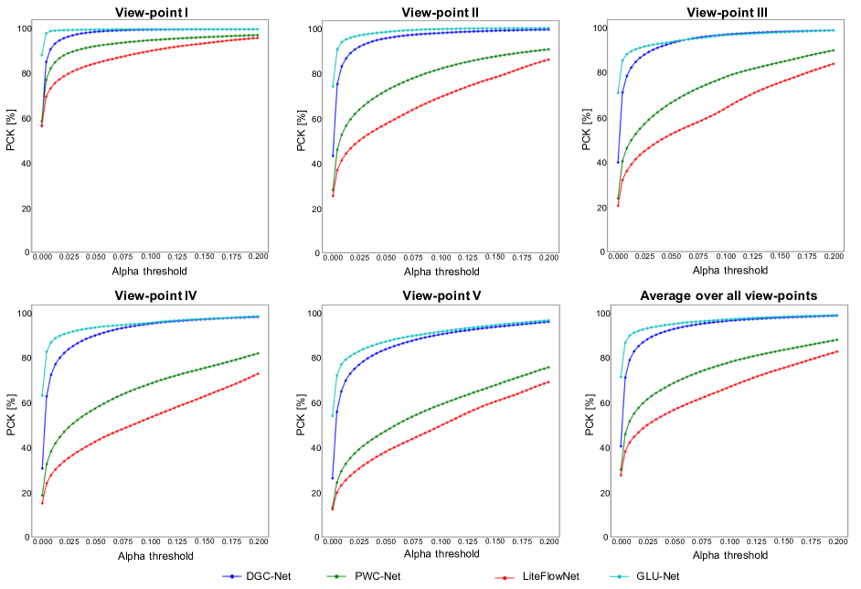
We additionally present the PCK curves computed over the different viewpoints of HP, as a function of the relative distance threshold. We do not set a pixel-level thresholds for the PCK curves since HP image pairs have different resolutions in general. GLU-Net achieves better accuracy (better PCK) for all thresholds compared to PWC-Net [57], LiteFLowNet [23] and DGC-Net [41]. Importantly, GLU-Net obtains significantly better PCK for low thresholds.

C.3.2 Results on ETH3D

In the main paper, Figure 5, we quantitatively evaluated our approach over pairs of ETH3D images sampled from consecutive frames at different intervals. In Table 9, we give the corresponding detailed evaluation metrics (AEPE and PCK) obtained by PWC-Net, LiteFlowNet, DGC-Net, DGC-Net^† and GLU-Net.

Note that the PCK and AEPE values computed per image are then averaged over all image pairs of each sequence. The final metrics presented are the averages over all sequences.

		LiteFlowNet	PWC-Net	DGC-Net	DGC-Net†	GLU-Net (Ours)
	AEPE	1.67	1.75	2.49	2.76	1.98
interval = 3	PCK-1px [%]	61.63	57.54	34.19	27.55	50.55
	PCK-5px [%]	92.79	92.62	88.50	86.65	91.22
	AEPE	2.58	2.10	3.28	3.61	2.54
interval = 5	PCK-1px [%]	56.55	50.41	27.22	21.23	43.08
	PCK-5px [%]	90.70	90.71	83.25	81.01	87.91
	AEPE	6.05	3.21	4.18	4.67	3.48
interval = 7	PCK-1px [%]	49.83	42.95	22.45	16.91	36.98
	PCK-5px [%]	86.29	87.04	78.32	75.50	84.23
	AEPE	12.95	5.59	5.35	5.61	4.23
interval = 9	PCK-1px [%]	42.00	35.23	18.82	13.91	32.45
	PCK-5px [%]	78.50	81.17	73.74	70.54	80.74
	AEPE	29.67	14.35	6.78	7.13	5.59
interval = 11	PCK-1px [%]	33.14	28.14	15.82	11.67	28.45
	PCK-5px [%]	66.07	71.91	69.23	65.48	76.84
	AEPE	52.41	27.49	9.02	8.89	7.54
interval = 13	PCK-1px [%]	26.46	22.91	13.49	9.82	25.06
	PCK-5px [%]	55.05	63.19	64.28	60.42	72.35
	AEPE	74.96	43.41	12.25	12.45	10.75
interval = 15	PCK-1px [%]	21.22	18.34	11.25	8.14	21.89
	PCK-5px [%]	46.29	54.39	58.66	54.69	67.77

Table 9: Metrics evaluated over scenes of ETH3D with different intervals between consecutive pairs of images (taken by the same camera). Note that those results are the average over the different sequences of the ETH3D dataset. Small AEPE and high PCK are better.

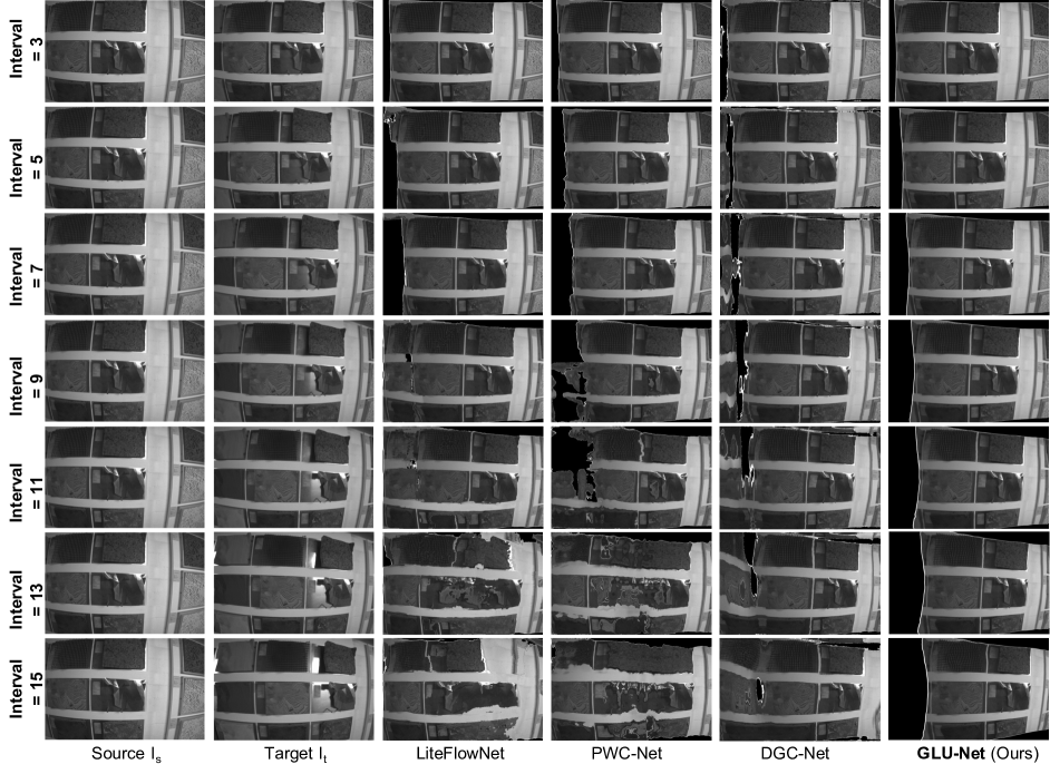
Here, we additionally provide qualitative examples of the different networks and GLU-Net applied to pairs of images at different intervals in Figure 13. It is visible that while optical flow methods achieve good results for low intervals, the warped source images according to their outputted flows get worst when increasing the intervals between image pairs. On the other hand, our model produces flow fields of constant quality.

Figure 10: Qualitative examples of state-of-the-art methods applied to very high-resolution images of different scenes of ETH3D. The presented image pairs show substantial view-point changes, and thus very large motions.

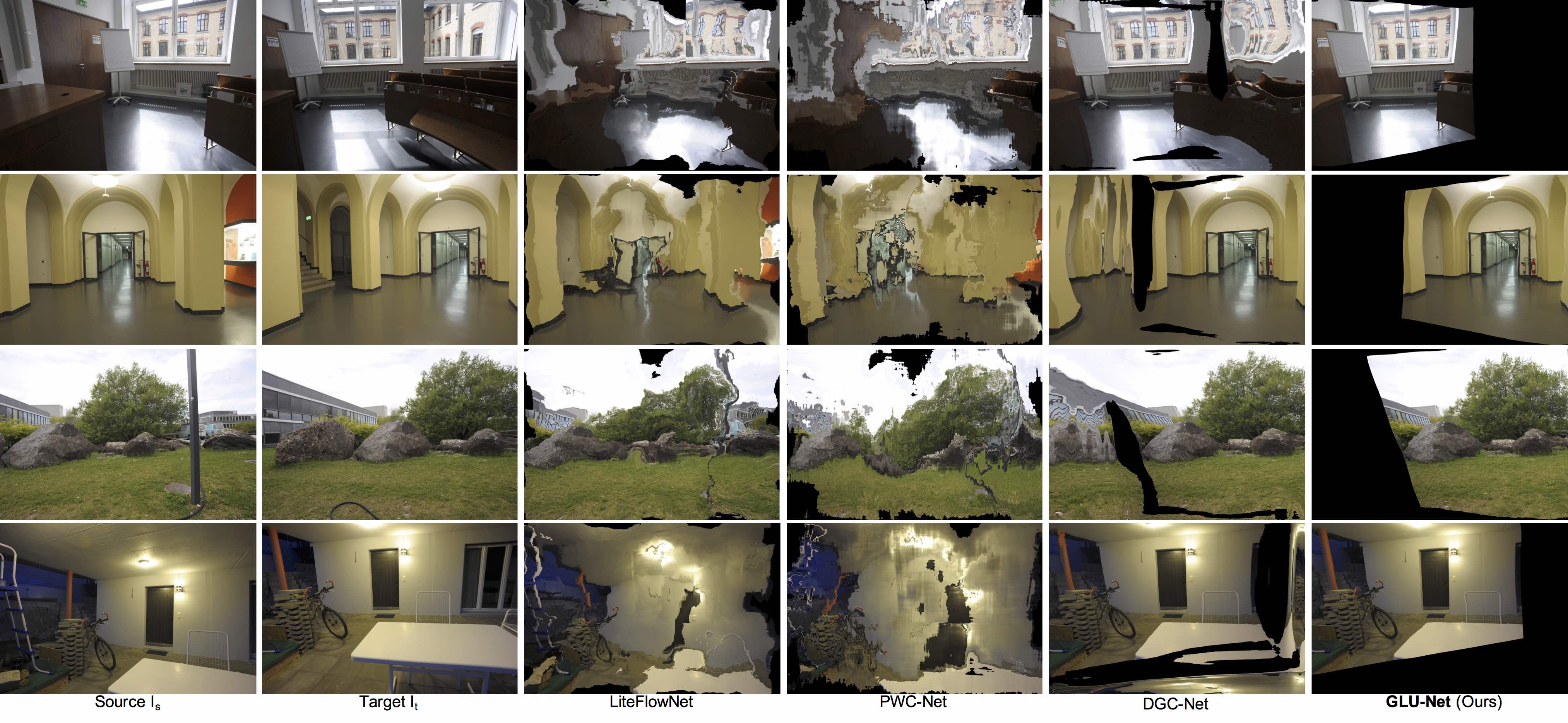
Qualitative results: We additionally use ETH3D images to demonstrate the superiority of our approach to deal with extreme viewpoint changes on the one hand, and radical illumination and appearance variations on the other hand.

In addition to the medium resolution images evaluated previously, ETH3D [53] also provides several additional scenes taken with high-resolution cameras, acquiring images at 24 Megapixel ($6048\times 4032$). Since the images of a sequence are taken by a unique camera, consecutive pairs of images show only little lightning variations, however they are related by very wide view-point changes. As there are no ground-truth correspondences provided along with the images, we only evaluate qualitatively on consecutive pairs of images. The original images of $6048\times 4032$ are down-samled by a factor of $2$ for practical purposes. We show quantitative results over a few of those images in Figure 10. GLU-Net is capable of handling very large motions, where the other methods partly (DGC-Net) or completely fail (PWC-Net and LiteFlowNet).

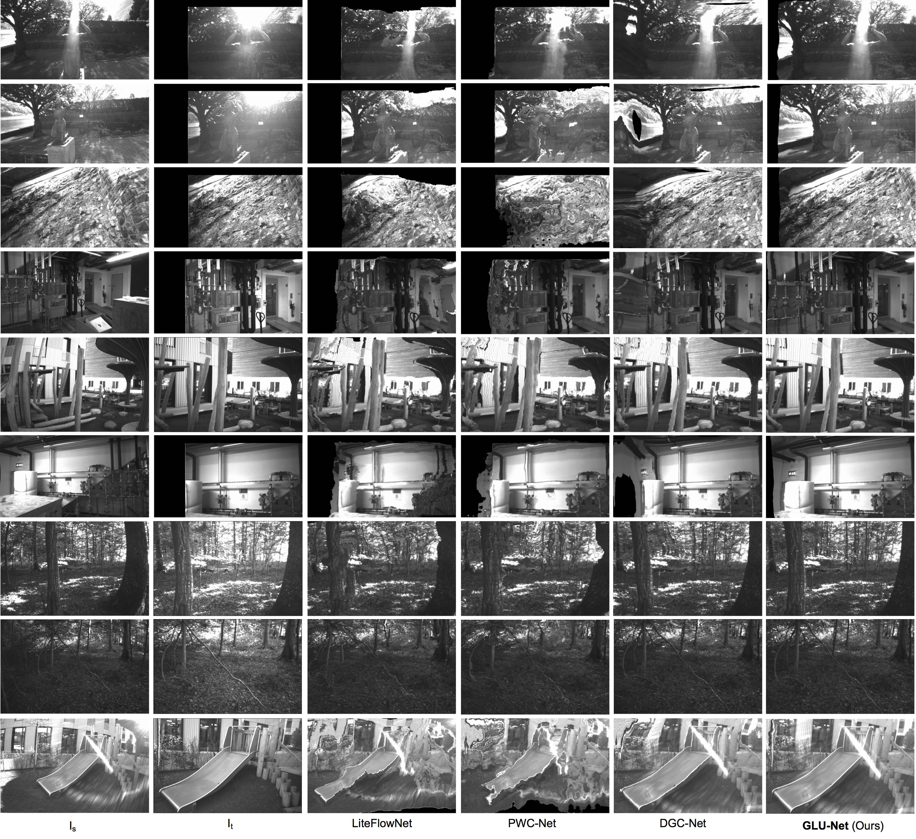
On the other hand, our network can also handle large appearances changes due to variation in illumination or due to the use of different optics. For this purpose, we utilize additional examples of pairs of images from ETH3D taken by two different cameras simultaneously. The camera of the first images has a field-of-view of 54 degrees while the other camera has a field of view of 83 degrees. They capture images at a resolution of $480\times 752$ or $514\times 955$ depending on the scenes and on the camera. The exposure settings of the cameras are set to automatic for all datasets, allowing the device to adapt to illumination changes. Qualitative examples of state-of-the-art methods and GLU-Net applied to such pairs of images are presented in Figure 12. GLU-Net is robust to changes in lightning conditions as well as to artifacts. While DGC-Net [41] obtains satisfactory results, the warped image according to its outputted flow is often blurry whereas we always obtain sharp, almost perfect warped source images.

Figure 11: Qualitative examples of different state-of-the-art algorithms and our GLU-Net applied to HP images. The source images are warped according to the flow fields outputted by the different networks. The warped source images should resemble the target images. Our method GLU-Net is robust to drastic view-point changes.

Figure 12: Qualitative examples of ETH3D pairs of images taken simultaneously by two different cameras. The two cameras have different field-of-views and sometimes different resolutions. Pairs of images experience drastic differences in lightning conditions. The source images are warped according to the flow fields outputted by different state-of-the-art networks and by our GLU-Net. The warped source images should resemble the target images.

Figure 13: Qualitative examples of multiple networks and our GLU-Net applied to pairs of ETH3D dataset taken at different intervals by the same camera. The source images are warped according to the flow fields outputted by the different networks. The warped source images should resemble the target images. Optical flow methods obtain good qualitative results for low intervals (3 and 5) but largely degrade on bigger intervals. On the contrary, GLU-Net has a steady performance over all intervals.

(A) Metrics with respect to rotation

(B) Metrics with respect to scaling

Figure 14: Quantitative results (AEPE, PCK-1px and PCK-5px) over the first viewpoint of HP, for different rotation and scaling factors applied to the target images and ground-truth flow fields. The training datasets are indicated in parenthesis for each model.

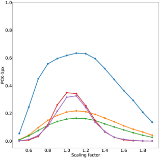
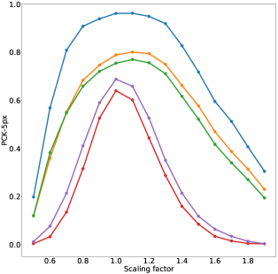
C.3.3 Rotation and scaling

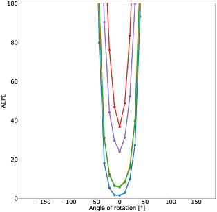
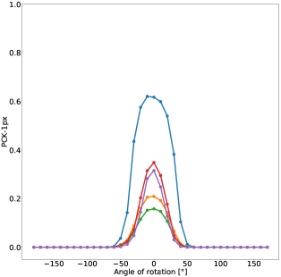
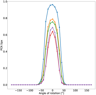
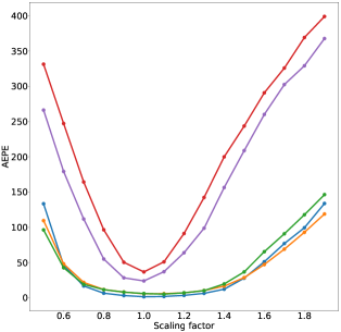
We additionally measured the performance of our GLU-Net compared to state-of-the-art networks with respect to increasing rotation and scaling factors. To do so, we used the 59 pairs of the ViewPoint I of the HP [5] dataset as base images and applied increasingly high rotation and scaling factors to the target and ground-truth flow fields. In Figure 14, we plot the metrics (AEPE, PCK-1px and PCK-5px) obtained by GLU-Net, DGC-Net, DGC-Net^†, PWC-Net and LiteFlowNet with respect to increasing applied rotation or scaling factors. For both rotation and scaling, while GLU-Net obtains similar AEPE than DGC-Net, its accuracy (PCK-1px and PCK-5px) is significantly above that of DGC-Net.

It must also be noted that GLU-Net is particularly robust and accurate for rotations up to +/- 50 degrees and scaling factors comprised between 0.8 and 1.4. This corresponds to the extent of geometric transformations present in the training dataset. Therefore, for improved robustness to larger rotations or scaling, image pairs experiencing such transformations should be additionally included in the training set.

C.4 Semantic correspondences

In Figure 17, we present additional qualitative results on the TSS [60] dataset of our universal network (GLU-Net) and its modified version (Semantic-GLU-Net), which includes NC-Net [49] and feature concatenation [30].

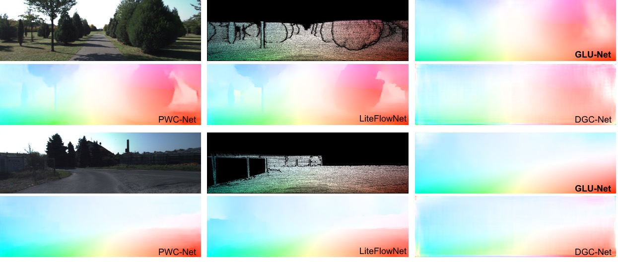
(A) KITTI-2012 dataset

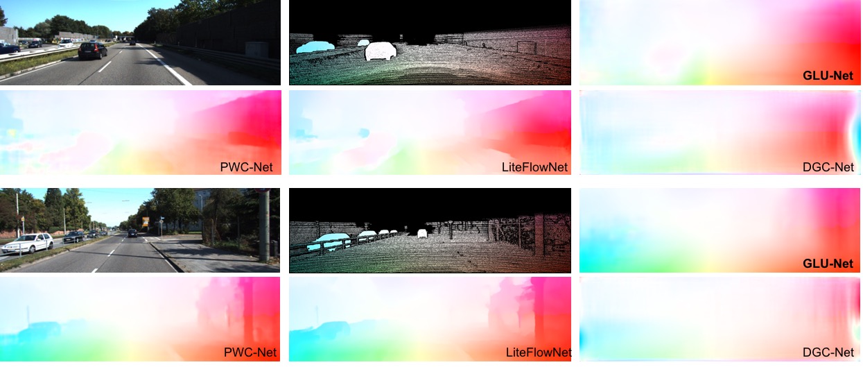
(B) KITTI-2015 dataset

Figure 15: Representation of the flow fields estimated by state-of-the-art methods and GLU-Net applied to images of : (A) KITTI 2012 dataset, that is restricted to static scenes; (B) KITTI 2015 dataset, which comprises dynamic scenes.

C.5 Optical flow

Additional qualitative results: In Figure 15, we present additional qualitative examples of the estimated flow fields obtained by our method and competitors on the KITTI datasets. While our approach GLU-Net lacks accuracy at the object boundaries compared to the optical flow methods, our results are substantially better than those of DGC-Net, which is trained on the same kind of synthetic geometric transformations. As already stated, improved results, particularly at the object boundaries, could be obtained by including optical flow data with independently moving objects in the training set.

Supplementary analysis of the optical flow results: According to Table 3 and Figure 5 of the main paper, our GLU-Net obtains better AEPE than the optical flow methods PWC-Net and LiteFlowNet on the KITTI datasets (Table 3), but worst AEPE on the first intervals of ETH3D (Figure  5). The reasons for this behavior are explained below. As observed in Figure 16, while KITTI and ETH3D pairs for small intervals show similar average displacement, the KITTI datasets have a much wider distribution of displacements due to moving objects and the fast camera forward motion. Besides, our GLU-Net performs substantially better on the large-displacement pixels of KITTI compared to

Figure 16: Ground-truth flow distribution (in log scale) for the ETH3D dataset sampled at small intervals and for the KITTI datasets.

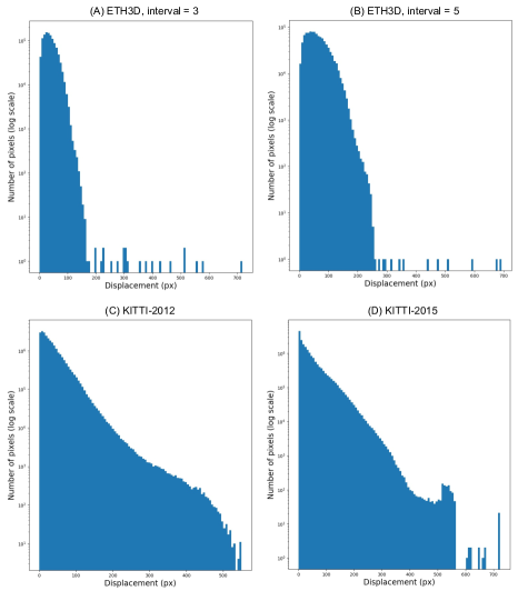
PWC-Net and LiteFlowNet, as evidenced in Table 10. This explains the on-average advantage of our approach (better AEPE), despite being slightly weaker for small displacements.

	KITTI-2012			KITTI-2015
	Small	Medium	Large	Small	Medium	Large
PWC-Net	0.63	1.58	10.36	0.94	2.89	28.65
LiteFlowNet	0.46	1.24	10.83	0.68	2.32	29.93
DGC-Net	1.53	3.10	21.90	3.44	6.48	36.07
GLU-Net	0.83	1.63	7.68	2.25	4.87	23.01

Table 10: AEPE for different ground truth pixel-displacement categories on the KITTI datasets. Small is defined as $\left\|\mathbf{w}_{GT}\right\|_{2}<10$, Medium as $10\leq\left\|\mathbf{w}_{GT}\right\|_{2}<40$ and Large as $40\leq\left\|\mathbf{w}_{GT}\right\|_{2}$. The EPE is averaged over all pixels of the dataset.

C.6 Detailed ablative analysis

In this section, we provide additional ablation experiments. All networks are trained on CityScape-DPED-ADE dataset.

Coarse-to-fine-approach: We first defend the use of a coarse-to-fine approach with a feature pyramid. We report AEPE and PCK metrics for the flow estimates obtained at different levels of the feature pyramid of GLU-Net model in Table 11. On the flow field estimated at each level, we apply bilinear interpolation to the original image resolution and multiply the estimated flow with the corresponding scale factor for the levels of L-Net. The end-point error decreases from the coarsest level to the highest level of the pyramid while the accuracy (PCK) increases. This supports the use of a pyramidal model.

Scale pyramid level of the adaptive resolution: In Table 12, we present the influence of the pyramid level at which the adaptive resolution module is integrated in the four-level pyramid network. Having a single level in L-Net (corresponding to the global correlation layer) and three pyramid levels in H-Net (referred to as 3L) lead to poor results on all datasets, even compared to GLOCAL-Net. On the other hand, both other alternatives (1 or 2 levels in H-Net) bring about major improvements of robustness (AEPE) and accuracy (PCK) on HPatches dataset, particularly on the high-resolution images HP. However, having only one level in H-Net (1L) degrades the performances obtained on the semantic dataset TSS. H-Net and L-Net both comprised of 2 pyramid levels (2L) appears as the best option to achieve competitive results on geometric matching, optical flow as well as semantic matching.

	AEPE	PCK-1px [%]	PCK-5px [%]
Level 1 [$16\times 16$]	45.49	0.70	13.53
Level 2 [$32\times 32$]	30.00	6.27	50.29
Level 3 [$H/8\times W/8$]	26.43	30.47	74.44
Level 4 [$H/4\times W/4$]	25.05	39.55	78.54

Table 11: Effect of coarse-to-fine approach for our GLU-Net: Metrics calculated over HP images. The flow estimated at each pyramid level is up-sampled to original image resolution and the metrics are calculated at this resolution.

		GLOCAL-Net	1L = 1 H-Net level	2L = 2 H-Net levels	3L = 3 H-Net levels
HP-240	AEPE	8.77	7.47	7.69	8.93
	PCK-1px [%]	48.53	62.85	53.83	35.81
	PCK-5px [%]	78.12	85.32	83.17	75.97
	AEPE	31.64	24.75	25.55	32.03
HP	PCK-1px [%]	10.23	33.92	35.26	28.76
	PCK-5px [%]	56.73	76.99	75.79	69.78
TSS	PCK [%]	77.29	62.98	78.97	69.78

Table 12: Effect of adaptive resolution and its position. All networks are without iterative refinement and without cyclic consistency. 2 H-Net levels (2L) is the only alternative for a universal network applicable to geometric matching, semantic correspondence and optical flow.

Figure 17: Qualitative examples of our universal network GLU-Net as well as GLU-Net with specific architectural details from the semantic correspondence literature applied to TSS images. The additional architectural modules are the Neighborhood Consensus Network NC-Net [49] and concatenating features within the L-Net [30]. Adopting those two modules leads to Semantic-GLU-Net. The source images are warped according to the flow fields outputted by the different networks. The warped source images should resemble the target images and the ground-truths.

References

- [1] Sameer Agarwal, Yasutaka Furukawa, Noah Snavely, Ian Simon, Brian Curless, Steven M. Seitz, and Richard Szeliski. Building rome in a day. Commun. ACM, 54(10):105–112, 2011.
- [2] Alexandre Alahi, Raphael Ortiz, and Pierre Vandergheynst. Freak: Fast retina keypoint. In CVPR, pages 510–517. IEEE Computer Society, 2012.
- [3] Pablo Fernández Alcantarilla, Adrien Bartoli, and Andrew J. Davison. Kaze features. In Andrew W. Fitzgibbon, Svetlana Lazebnik, Pietro Perona, Yoichi Sato, and Cordelia Schmid, editors, ECCV (6), volume 7577 of Lecture Notes in Computer Science, pages 214–227. Springer, 2012.
- [4] Simon Baker, Daniel Scharstein, J. P. Lewis, Stefan Roth, Michael J. Black, and Richard Szeliski. A database and evaluation methodology for optical flow. International Journal of Computer Vision, 92(1):1–31, 2011.
- [5] Vassileios Balntas, Karel Lenc, Andrea Vedaldi, and Krystian Mikolajczyk. Hpatches: A benchmark and evaluation of handcrafted and learned local descriptors. In 2017 IEEE Conference on Computer Vision and Pattern Recognition, CVPR 2017, Honolulu, HI, USA, July 21-26, 2017, pages 3852–3861, 2017.
- [6] Herbert Bay, Tinne Tuytelaars, and Luc Van Gool. SURF: speeded up robust features. In Computer Vision - ECCV 2006, 9th European Conference on Computer Vision, Graz, Austria, May 7-13, 2006, Proceedings, Part I, pages 404–417, 2006.
- [7] Daniel J. Butler, Jonas Wulff, Garrett B. Stanley, and Michael J. Black. A naturalistic open source movie for optical flow evaluation. In Computer Vision - ECCV 2012 - 12th European Conference on Computer Vision, Florence, Italy, October 7-13, 2012, Proceedings, Part VI, pages 611–625, 2012.
- [8] K. Chatfield, K. Simonyan, A. Vedaldi, and A. Zisserman. Return of the devil in the details: Delving deep into convolutional nets. In BMVC, 2014.
- [9] Liang-Chieh Chen, George Papandreou, Florian Schroff, and Hartwig Adam. Rethinking atrous convolution for semantic image segmentation. CoRR, abs/1706.05587, 2017.
- [10] Christopher Bongsoo Choy, JunYoung Gwak, Silvio Savarese, and Manmohan Krishna Chandraker. Universal correspondence network. In Advances in Neural Information Processing Systems 29: Annual Conference on Neural Information Processing Systems 2016, December 5-10, 2016, Barcelona, Spain, pages 2406–2414, 2016.
- [11] Marius Cordts, Mohamed Omran, Sebastian Ramos, Timo Rehfeld, Markus Enzweiler, Rodrigo Benenson, Uwe Franke, Stefan Roth, and Bernt Schiele. The cityscapes dataset for semantic urban scene understanding. In Proc. of the IEEE Conference on Computer Vision and Pattern Recognition (CVPR), 2016.
- [12] Daniel DeTone, Tomasz Malisiewicz, and Andrew Rabinovich. Superpoint: Self-supervised interest point detection and description. In 2018 IEEE Conference on Computer Vision and Pattern Recognition Workshops, CVPR Workshops 2018, Salt Lake City, UT, USA, June 18-22, 2018, pages 224–236, 2018.
- [13] Alexey Dosovitskiy, Philipp Fischer, Eddy Ilg, Philip Häusser, Caner Hazirbas, Vladimir Golkov, Patrick van der Smagt, Daniel Cremers, and Thomas Brox. Flownet: Learning optical flow with convolutional networks. In 2015 IEEE International Conference on Computer Vision, ICCV 2015, Santiago, Chile, December 7-13, 2015, pages 2758–2766, 2015.
- [14] David A. Forsyth and Jean Ponce. Computer Vision - A Modern Approach, Second Edition. Pitman, 2012.
- [15] Andreas Geiger, Philip Lenz, Christoph Stiller, and Raquel Urtasun. Vision meets robotics: The kitti dataset. I. J. Robotic Res., 32(11):1231–1237, 2013.
- [16] Yoav HaCohen, Eli Shechtman, Dan B. Goldman, and Dani Lischinski. Non-rigid dense correspondence with applications for image enhancement. ACM Trans. Graph., 30(4):70, 2011.
- [17] Bumsub Ham, Minsu Cho, Cordelia Schmid, and Jean Ponce. Proposal flow: Semantic correspondences from object proposals. IEEE Trans. Pattern Anal. Mach. Intell., 40(7):1711–1725, 2018.
- [18] Andrew Harltey and Andrew Zisserman. Multiple view geometry in computer vision (2. ed.). Cambridge University Press, 2006.
- [19] Christopher G. Harris and Mike Stephens. A combined corner and edge detector. In Proceedings of the Alvey Vision Conference, AVC 1988, Manchester, UK, September, 1988, pages 1–6, 1988.
- [20] Berthold K. P. Horn and Brian G. Schunck. ”determining optical flow”: A retrospective. Artif. Intell., 59(1-2):81–87, 1993.
- [21] Gao Huang, Zhuang Liu, Laurens van der Maaten, and Kilian Q. Weinberger. Densely connected convolutional networks. In 2017 IEEE Conference on Computer Vision and Pattern Recognition, CVPR 2017, Honolulu, HI, USA, July 21-26, 2017, pages 2261–2269. IEEE Computer Society, 2017.
- [22] Shuaiyi Huang, Qiuyue Wang, Songyang Zhang, Shipeng Yan, and Xuming He. Dynamic context correspondence network for semantic alignment. In 2019 IEEE/CVF International Conference on Computer Vision, ICCV 2019, Seoul, Korea (South), October 27 - November 2, 2019, pages 2010–2019. IEEE, 2019.
- [23] Tak-Wai Hui, Xiaoou Tang, and Chen Change Loy. Liteflownet: A lightweight convolutional neural network for optical flow estimation. In 2018 IEEE Conference on Computer Vision and Pattern Recognition, CVPR 2018, Salt Lake City, UT, USA, June 18-22, 2018, pages 8981–8989, 2018.
- [24] Tak-Wai Hui, Xiaoou Tang, and Chen Change Loy. A Lightweight Optical Flow CNN - Revisiting Data Fidelity and Regularization. 2020.
- [25] Andrey Ignatov, Nikolay Kobyshev, Radu Timofte, Kenneth Vanhoey, and Luc Van Gool. Dslr-quality photos on mobile devices with deep convolutional networks. In IEEE International Conference on Computer Vision, ICCV 2017, Venice, Italy, October 22-29, 2017, pages 3297–3305, 2017.
- [26] Eddy Ilg, Nikolaus Mayer, Tonmoy Saikia, Margret Keuper, Alexey Dosovitskiy, and Thomas Brox. Flownet 2.0: Evolution of optical flow estimation with deep networks. In 2017 IEEE Conference on Computer Vision and Pattern Recognition, CVPR 2017, Honolulu, HI, USA, July 21-26, 2017, pages 1647–1655. IEEE Computer Society, 2017.
- [27] Sergey Ioffe and Christian Szegedy. Batch normalization: Accelerating deep network training by reducing internal covariate shift. In Proceedings of the 32nd International Conference on Machine Learning, ICML 2015, Lille, France, 6-11 July 2015, pages 448–456, 2015.
- [28] Max Jaderberg, Karen Simonyan, Andrew Zisserman, and Koray Kavukcuoglu. Spatial transformer networks. In Advances in Neural Information Processing Systems 28: Annual Conference on Neural Information Processing Systems 2015, December 7-12, 2015, Montreal, Quebec, Canada, pages 2017–2025, 2015.
- [29] Joel Janai, Fatma Güney, Aseem Behl, and Andreas Geiger. Computer vision for autonomous vehicles: Problems, datasets and state-of-the-art. CoRR, abs/1704.05519, 2017.
- [30] Sangryul Jeon, Seungryong Kim, Dongbo Min, and Kwanghoon Sohn. PARN: pyramidal affine regression networks for dense semantic correspondence. In Computer Vision - ECCV 2018 - 15th European Conference, Munich, Germany, September 8-14, 2018, Proceedings, Part VI, pages 355–371, 2018.
- [31] Seungryong Kim, Stephen Lin, Sangryul Jeon, Dongbo Min, and Kwanghoon Sohn. Recurrent transformer networks for semantic correspondence. In Advances in Neural Information Processing Systems 31: Annual Conference on Neural Information Processing Systems 2018, NeurIPS 2018, 3-8 December 2018, Montréal, Canada., pages 6129–6139, 2018.
- [32] Seungryong Kim, Dongbo Min, Bumsub Ham, Stephen Lin, and Kwanghoon Sohn. FCSS: fully convolutional self-similarity for dense semantic correspondence. IEEE Trans. Pattern Anal. Mach. Intell., 41(3):581–595, 2019.
- [33] Seungryong Kim, Dongbo Min, Somi Jeong, Sunok Kim, Sangryul Jeon, and Kwanghoon Sohn. Semantic attribute matching networks. In IEEE Conference on Computer Vision and Pattern Recognition, CVPR 2019, Long Beach, CA, USA, June 16-20, 2019, pages 12339–12348, 2019.
- [34] Diederik P. Kingma and Jimmy Ba. Adam: A method for stochastic optimization. In 3rd International Conference on Learning Representations, ICLR 2015, San Diego, CA, USA, May 7-9, 2015, Conference Track Proceedings, 2015.
- [35] Alex Krizhevsky, Ilya Sutskever, and Geoffrey E. Hinton. Imagenet classification with deep convolutional neural networks. In Advances in Neural Information Processing Systems 25: 26th Annual Conference on Neural Information Processing Systems 2012. Proceedings of a meeting held December 3-6, 2012, Lake Tahoe, Nevada, United States., pages 1106–1114, 2012.
- [36] Zakaria Laskar, Iaroslav Melekhov, Hamed R. Tavakoli, Juha Ylioinas, and Juho Kannala. Geometric image correspondence verification by dense pixel matching. CoRR, abs/1904.06882, 2019.
- [37] Stefan Leutenegger, Margarita Chli, and Roland Siegwart. BRISK: binary robust invariant scalable keypoints. In IEEE International Conference on Computer Vision, ICCV 2011, Barcelona, Spain, November 6-13, 2011, pages 2548–2555, 2011.
- [38] Ce Liu, Jenny Yuen, and Antonio Torralba. SIFT flow: Dense correspondence across scenes and its applications. IEEE Trans. Pattern Anal. Mach. Intell., 33(5):978–994, 2011.
- [39] David G. Lowe. Distinctive image features from scale-invariant keypoints. International Journal of Computer Vision, 60(2):91–110, 2004.
- [40] Nikolaus Mayer, Eddy Ilg, Philipp Fischer, Caner Hazirbas, Daniel Cremers, Alexey Dosovitskiy, and Thomas Brox. What makes good synthetic training data for learning disparity and optical flow estimation? International Journal of Computer Vision, 126(9):942–960, 2018.
- [41] Iaroslav Melekhov, Aleksei Tiulpin, Torsten Sattler, Marc Pollefeys, Esa Rahtu, and Juho Kannala. DGC-Net: Dense geometric correspondence network. In Proceedings of the IEEE Winter Conference on Applications of Computer Vision (WACV), 2019.
- [42] Vinod Nair and Geoffrey E. Hinton. Rectified linear units improve restricted boltzmann machines. In Proceedings of the 27th International Conference on Machine Learning (ICML-10), June 21-24, 2010, Haifa, Israel, pages 807–814, 2010.
- [43] Simon Niklaus. A reimplementation of LiteFlowNet using PyTorch. https://github.com/sniklaus/pytorch-liteflownet, 2019.
- [44] Yuki Ono, Eduard Trulls, Pascal Fua, and Kwang Moo Yi. Lf-net: Learning local features from images. In Advances in Neural Information Processing Systems 31: Annual Conference on Neural Information Processing Systems 2018, NeurIPS 2018, 3-8 December 2018, Montréal, Canada, pages 6237–6247, 2018.
- [45] Adam Paszke, Sam Gross, Soumith Chintala, Gregory Chanan, Edward Yang, Zachary DeVito, Zeming Lin, Alban Desmaison, Luca Antiga, and Adam Lerer. Automatic differentiation in PyTorch. In NIPS Autodiff Workshop, 2017.
- [46] Anurag Ranjan and Michael J. Black. Optical flow estimation using a spatial pyramid network. In 2017 IEEE Conference on Computer Vision and Pattern Recognition, CVPR 2017, Honolulu, HI, USA, July 21-26, 2017, pages 2720–2729, 2017.
- [47] Ignacio Rocco, Relja Arandjelovic, and Josef Sivic. Convolutional neural network architecture for geometric matching. In 2017 IEEE Conference on Computer Vision and Pattern Recognition, CVPR 2017, Honolulu, HI, USA, July 21-26, 2017, pages 39–48, 2017.
- [48] Ignacio Rocco, Relja Arandjelovic, and Josef Sivic. End-to-end weakly-supervised semantic alignment. In 2018 IEEE Conference on Computer Vision and Pattern Recognition, CVPR 2018, Salt Lake City, UT, USA, June 18-22, 2018, pages 6917–6925, 2018.
- [49] Ignacio Rocco, Mircea Cimpoi, Relja Arandjelovic, Akihiko Torii, Tomás Pajdla, and Josef Sivic. Neighbourhood consensus networks. In Advances in Neural Information Processing Systems 31: Annual Conference on Neural Information Processing Systems 2018, NeurIPS 2018, 3-8 December 2018, Montréal, Canada., pages 1658–1669, 2018.
- [50] Ethan Rublee, Vincent Rabaud, Kurt Konolige, and Gary R. Bradski. ORB: an efficient alternative to SIFT or SURF. In IEEE International Conference on Computer Vision, ICCV 2011, Barcelona, Spain, November 6-13, 2011, pages 2564–2571, 2011.
- [51] Johannes L. Schönberger and Jan-Michael Frahm. Structure-from-motion revisited. In 2016 IEEE Conference on Computer Vision and Pattern Recognition, CVPR 2016, Las Vegas, NV, USA, June 27-30, 2016, pages 4104–4113, 2016.
- [52] Johannes L. Schönberger, Marc Pollefeys, Andreas Geiger, and Torsten Sattler. Semantic visual localization. In 2018 IEEE Conference on Computer Vision and Pattern Recognition, CVPR 2018, Salt Lake City, UT, USA, June 18-22, 2018, pages 6896–6906. IEEE Computer Society, 2018.
- [53] Thomas Schöps, Johannes L. Schönberger, Silvano Galliani, Torsten Sattler, Konrad Schindler, Marc Pollefeys, and Andreas Geiger. A multi-view stereo benchmark with high-resolution images and multi-camera videos. In 2017 IEEE Conference on Computer Vision and Pattern Recognition, CVPR 2017, Honolulu, HI, USA, July 21-26, 2017, pages 2538–2547, 2017.
- [54] René Schuster, Oliver Wasenmüller, Christian Unger, and Didier Stricker. An empirical evaluation study on the training of SDC features for dense pixel matching. In IEEE Conference on Computer Vision and Pattern Recognition Workshops, CVPR Workshops 2019, Long Beach, CA, USA, June 16-20, 2019, page 0, 2019.
- [55] Karen Simonyan and Andrew Zisserman. Two-stream convolutional networks for action recognition in videos. CoRR, abs/1406.2199, 2014.
- [56] Rainer Sprengel, Karl Rohr, and H. Siegfried Stiehl. Thin-plate spline approximation for image registration. In Annual International Conference of the IEEE Engineering in Medicine and Biology - Proceedings, 1996.
- [57] Deqing Sun, Xiaodong Yang, Ming-Yu Liu, and Jan Kautz. Pwc-net: Cnns for optical flow using pyramid, warping, and cost volume. In 2018 IEEE Conference on Computer Vision and Pattern Recognition, CVPR 2018, Salt Lake City, UT, USA, June 18-22, 2018, pages 8934–8943, 2018.
- [58] Deqing Sun, Xiaodong Yang, Ming-Yu Liu, and Jan Kautz. Models matter, so does training: An empirical study of cnns for optical flow estimation. IEEE transactions on pattern analysis and machine intelligence, 2019.
- [59] Hajime Taira, Masatoshi Okutomi, Torsten Sattler, Mircea Cimpoi, Marc Pollefeys, Josef Sivic, Tomás Pajdla, and Akihiko Torii. Inloc: Indoor visual localization with dense matching and view synthesis. In 2018 IEEE Conference on Computer Vision and Pattern Recognition, CVPR 2018, Salt Lake City, UT, USA, June 18-22, 2018, pages 7199–7209. IEEE Computer Society, 2018.
- [60] Tatsunori Taniai, Sudipta N. Sinha, and Yoichi Sato. Joint recovery of dense correspondence and cosegmentation in two images. In 2016 IEEE Conference on Computer Vision and Pattern Recognition, CVPR 2016, Las Vegas, NV, USA, June 27-30, 2016, pages 4246–4255, 2016.
- [61] Prune Truong. GLU-Net: Github project page. https://github.com/PruneTruong/GLU-Net, 2020.
- [62] Prune Truong, Stefanos Apostolopoulos, Agata Mosinska, Samuel Stucky, Carlos Ciller, and Sandro De Zanet. Glampoints: Greedily learned accurate match points. 2019 IEEE/CVF International Conference on Computer Vision (ICCV), pages 10731–10740, 2019.
- [63] Pascal Vincent, Hugo Larochelle, Yoshua Bengio, and Pierre-Antoine Manzagol. Extracting and composing robust features with denoising autoencoders. In Machine Learning, Proceedings of the Twenty-Fifth International Conference (ICML 2008), Helsinki, Finland, June 5-9, 2008, pages 1096–1103, 2008.
- [64] Bolei Zhou, Hang Zhao, Xavier Puig, Tete Xiao, Sanja Fidler, Adela Barriuso, and Antonio Torralba. Semantic understanding of scenes through the ADE20K dataset. Int. J. Comput. Vis., 127(3):302–321, 2019.