The Wasserstein-Fourier Distance
for Stationary Time Series

Abstract

We propose the Wasserstein-Fourier (WF) distance to measure the (dis)similarity between time series by quantifying the displacement of their energy across frequencies. The WF distance operates by calculating the Wasserstein distance between the (normalised) power spectral densities (NPSD) of time series. Yet this rationale has been considered in the past, we fill a gap in the open literature providing a formal introduction of this distance, together with its main properties from the joint perspective of Fourier analysis and optimal transport. As the main aim of this work is to validate WF as a general-purpose metric for time series, we illustrate its applicability on three broad contexts. First, we rely on WF to implement a PCA-like dimensionality reduction for NPSDs which allows for meaningful visualisation and pattern recognition applications. Second, we show that the geometry induced by WF on the space of NPSDs admits a geodesic interpolant between time series, thus enabling data augmentation on the spectral domain, by averaging the dynamic content of two signals. Third, we implement WF for time series classification using parametric/non-parametric classifiers and compare it to other classical metrics. Supported on theoretical results, as well as synthetic illustrations and experiments on real-world data, this work establishes WF as a meaningful and capable resource pertinent to general distance-based applications of time series.

1 Introduction

Time series analysis is ubiquitous in a number of applications: from seismology to audio enhancement, from astronomy to fault detection, and from underwater navigation to source separation. Time series analysis occurs naturally in the spectral domain, where signals are represented in terms of how their energy is spread across frequencies. The spectral content of a signal is given by its—e.g., Fourier—power spectral density (PSD), which can be computed via the Periodogram [44] or parametric approaches such as the autoregressive and Yule-Walker methods [59, 54]. Comparing time series through their respective PSDs has been considered since the late 1960’s, e.g., using the Itakura-Saito (IS) distance [29] given by the Bregman divergence associated to the logarithm function between PSDs. Today, comparing time series in the spectral domain is still relevant mainly due to the recent advances on spectral estimation that are robust to noise, missing values, and general acquisition artefacts [49, 19, 55, 6, 46]. However, the IS divergence (as well as most distances between functions) is of no use when the spectral supports of the functions differ. Therefore, developing sound metrics for comparing general PSDs remains essential.

Beyond the realm of spectral analysis, the de facto tool for comparing general densities are Bregman divergences [2, 8]. The most popular one being the Kullback-Leibler (KL) divergence, which requires that one distribution dominates the other. To a lesser extent, the Euclidean distance has also been used for general-purpose comparison of distributions. In this article, we claim that the KL, IS and Euclidean distances have a fundamental drawback when comparing distributions of power, and thus they impose stringent requirements on the densities under study. In particular, these distances are only meaningful when the densities share a common support. In a nutshell, our point of view follows from the fact that the KL, IS and Euclidean distances are vertical divergences, meaning that they compare the (point-wise) values of two distributions for a given location in the $x$-axis (frequency). We, however, focus on how spectral energy is distributed across different values of the $x$-axis, thus requiring a horizontal distance. Fig. 1 illustrates the differences between a vertical and a horizontal distance using two Gaussians: observe that when these Gaussians become farther apart, the vertical distance becomes insensitive, whereas the horizontal one faithfully represents the displacement regardless of how far apart the densities are.

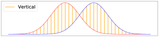
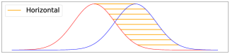
Figure 1: Vertical (top) and horizontal (bottom) displacements of two Gaussian distributions.

With the objective of building a meaningful, horizontal, spectral distance between time series, we rely on optimal transport (OT) and in particular on the Wasserstein distance [53], which is given by the cost of the optimal transportation (OT) between two probability distributions. This distance has already proven successful in a number of unsupervised learning applications such as clustering (of distributions) [58], generative adversarial networks [5] and Bayesian model selection [7]. Using probability distances for PSDs is also supported by the work of Basseville in [9], who in the late 1980’s had already categorised the distances for PSDs as probability based or frequency based. In the same line, the use of the Wasserstein distance on the space of PSDs is not new, related works include those of Flamary et al. in [25], which built a dictionary of fundamental and harmonic frequencies thus emphasising the importance of moving mass along the frequency dimension, and also [41], that followed the same rationale for supervised speech blind source separation. However, besides specific-purpose previous works, the open literature is still lacking a systematic study of the properties of this distance and its competence in general-purpose time series applications.

Contributions. Our hypothesis is that a rigorous framework for applying the Wasserstein distance to Fourier (power) representations, as well as understanding its geometric and statistical properties, would lay the foundations for developing novel tools for time series analysis. In that sense, the main contribution of this article is to propose an alternative, largely unexplored so far, general-purpose distance between time series based on OT. Additionally, specific contributions that are, to the best of our knowledge, novel in the literature include:

• The formal definition of the Wasserstein-Fourier (WF) distance and presentation of properties derived from a joint OT and spectral analysis standpoint (Sec. 3.1)

• The convergence behaviour of the WF distance and how it relates to the convergence of autocorrelation functions (Sec. 3.2, Prop. 1)

• A geodesic, i.e., minimum-cost, interpolant between time series based on the WF distance. This interpolation reveals the dynamic evolution between signals, and can be used for data augmentation (Sec. 4)

• A PCA-like dimensionality reduction technique based on the WF distance, specially suited for spectral representations, that allows for visualisation and pattern recognition (Sec. 5)

• A set of classifiers for time series by equipping standard parametric/non-parametric classifiers with the WF distance (Sec. 6)

• All the above conceptual packages are equipped with practical validation on illustrative synthetic examples and real-world data throughout the paper. The code to reproduce the experiments is available in Python at https://github.com/GAMES-UChile/Wasserstein-Fourier.

Organisation. The rest of this article is organised as follows. Section 2 presents the technical background for Fourier analysis and OT required to present our contribution. Then, Section 3 presents the proposed Wasserstein-Fourier distance and analyses its properties from OT and Signal Processing perspectives. Sections 4, 5 and 6 are devoted to the validation of the proposed distance through the three distance-based sets of experiments using synthetic and real-world datasets: interpolation paths between time series (and Gaussian processes), spectral dimensionality reduction and parametric/non-parametric regression. The paper then concludes with an assessment of our findings and a proposal for future research activities.

2 Background, assumptions and desiderata

2.1 An equivalence class for time series

We consider Fourier PSDs [30], based on the Fourier transform given by $\hat{x}(\xi)=\int_{-\infty}^{\infty}x(t)e^{-j2\pi\xi t}{\text{d}t}$ (we denote by $j$ the imaginary unit). The Fourier PSD for the continuous-time, stationary, stochastic time series $x(t)$ considered in this work is then given by

$$S(\xi)=\lim_{T\rightarrow\infty}\mathbb{E}\left[\frac{1}{2T}\left|\int_{-T}^{T}x(t)e^{-j2\pi t\xi}{\text{d}}t\right|^{2}\right].$$ (1)

Remark 1.

Though our work is presented for in the continuous-time, univariate, Fourier setting, the proposed WF distance can be applied to multivariate input, discrete time and arbitrary spectral domains. Critically, the WF distance is able to compare discrete-time signals against continuous-time ones. The only requirement of our method is that the spectral energy exists and it is finite, for instance, in the discrete-time case this translates to absolute summability and stationarity. Furthermore, the scope of our work is on wide-sense stationary signals, henceforth referred to as stationary.

We consider a unit-norm version of the Fourier PSD termed normalised power spectral density (NPSD) given by

$$s(\xi)=\frac{S(\xi)}{\int S(\xi^{\prime}){\text{d}}\xi^{\prime}}.$$ (2)

The justification for this choice is twofold. First, representing time series by a NPSD allows us to exploit the vast literature on divergences for probability distributions. Second, to compare the dynamic content of time series, i.e., how they evolve in time, the magnitude of the time series is irrelevant and so is the magnitude of its PSD (due to the linearity of the Fourier transform).

Choosing NPSDs and neglecting both the signal’s power and phase makes our representation blind to time-shifts (phase) and scaling. For stochastic processes, this representation has an interesting interpretation: as the PSD of a stationary stochastic process is uniquely linked to its covariance kernel (via Bochner’s theorem [13]), all processes with proportional kernels will have the same NPSD representation. This is particularly useful for Gaussian process (GPs, [39]), as it allows us to define a proper distance between GPs—see Sec. 4.5.

The NPSD representation thus induces an equivalence class for time series, denoted by $[x]=\{x^{\prime}|s_{x^{\prime}}=s_{x}\}$, where $s_{x}$ denotes the NPSD of $x$. The NPSD is then a non-injective embedding (or projection) from the space of time series onto the space of probability distributions due to the unit-norm choice. Time series belonging to the same equivalence class are thus understood to have the same dynamic content. As a consequence, we can define a distance between two (equivalence) classes of time series as the distance between their corresponding NPSDs, where the latter can be chosen as a divergence for probability distributions such as the Euclidean, Kullback-Leibler or Itakura-Saito divergences. In this work, we consider the Wasserstein distance instead.

2.2 Optimal transport

Optimal transport (OT, [53]) compares two probability distributions paying special attention to the geometry of their domain. This comparison is achieved by finding the lowest cost to transfer the mass from one probability distribution onto the other. Specifically, the optimal transport between two measures $\mu$ and $\nu$ defined on ${\mathbb{R}}^{d}$ is given by

$$\underset{\pi\in\Pi(\mu,\nu)}{\min}\int_{{\mathbb{R}}^{d}\times{\mathbb{R}}^{d}}c(x,y){\text{d}}\pi(x,y),$$ (3)

where $\pi$ is a joint distribution for $x$ and $y$, referred to as the transport plan, belonging to the space $\Pi(\mu,\nu)$ of the product measures on ${\mathbb{R}}^{d}\times{\mathbb{R}}^{d}$ with marginals $\mu$ and $\nu$; and $c:{\mathbb{R}}^{d}\times{\mathbb{R}}^{d}\mapsto{\mathbb{R}}$ is a cost function. In this manuscript, we focus on the Wasserstein distance, or Earth Mover’s distance [42], which is obtained by setting $c(x,y)=\|x-y\|^{p}$, $p\geq 1$, in eq. (3). This distance, denoted by

$$W_{p}(\mu,\nu)=\left(\underset{\pi\in\Pi(\mu,\nu)}{\min}\int_{{\mathbb{R}}^{d}\times{\mathbb{R}}^{d}}\|x-y\|^{p}{\text{d}}\pi(x,y)\right)^{1/p},$$ (4)

metrises the space $\mathcal{P}_{p}({\mathbb{R}}^{d})$ of measures admitting moments of order $p\geq 1$. Remarkably, OT immediately addresses the key challenge highlighted in Sec. 1, as it allows us to compare meaningfully continuous and discrete densities of different supports unlike the Euclidean distance and KL and IS divergences.

Additionally, notice that for one-dimensional probability measures—such as the NPSDs of a one dimensional signal, the optimisation (4) is closed-form and boils down to

$$W_{p}(\mu,\nu)=\left(\int_{0}^{1}|F^{-}_{\mu}(t)-F^{-}_{\nu}(t)|^{p}{\text{d}}t\right)^{1/p},$$ (5)

where $F^{-}_{\mu}$ represents the inverse cumulative function of $\mu\in\mathcal{P}_{p}({\mathbb{R}})$; this means that the calculation of the 1D Wasserstein distance is computationally inexpensive. We refer the reader to [53] for a theoretical presentation of OT and to [37] for recent computational aspects.

3 A Wasserstein-based distance between
Fourier power spectra

Let us consider the stationary signals $x$ and $y$ belonging to two classes of time series denoted by $[x]$ and $[y]$ respectively.

Definition 1.

The Wasserstein-Fourier (WF) distance between two equivalence classes of time series $[x]$ and $[y]$ is given by

$$\operatorname{WF}\left(\left[x\right],\left[y\right]\right)=W_{2}(s_{x},s_{y}),$$ (6)

where $s_{x}$ and $s_{y}$ denote the NPSDs associated to $[x]$ and $[y]$ respectively, as defined in eq. (2).

Note that by a slight abuse of notation, $s_{x}$ denotes both the probability density (or mass) function and the measure itself.

Remark 2.

The proposed WF distance holds for multi-dimensional signals, as long as their NPSDs exist. The contributions of this paper can then be straightforwardly applied to multi-dimensional signals, by considering NPSDs that are distributions supported on ${\mathbb{R}}^{d},d>1$, and for which the Wasserstein distance can be computed. However, in most time series applications presented here, such as the experiments in Sec. 4, 5 and 6, it is only needed to compute PSDs of uni-dimensional data. In such cases, the computational cost of the proposed WF distance is only of linear order.

Since the function $\operatorname{WF}(\cdot,\cdot)$ inherits the properties of the Wasserstein distance, we directly obtain the following result.

Theorem 1.

$\operatorname{WF}(\cdot,\cdot)$ is a distance over the space of equivalence classes of time series.

Proof.

The proof follows from the properties of the $W_{2}$ distance. For three arbitrary time series $x\in[x]$, $y\in[y]$ and $z\in[z]$, WF verifies:
(i) non-negativity: $\operatorname{WF}\left(\left[x\right],\left[y\right]\right)\geq 0$ is direct by the non-negativity of $W_{2}$,
(ii) identity of indiscernible: $\operatorname{WF}\left(\left[x\right],\left[y\right]\right)=W_{2}(s_{x},s_{y})=0$ is equivalent to $s_{x}=s_{y}$, and by definition of the equivalence class, to $[x]=[y]$,
(iii) symmetry: $\operatorname{WF}\left(\left[x\right],\left[y\right]\right)=W_{2}(s_{x},s_{y})=W_{2}(s_{y},s_{x})=\operatorname{WF}\left(\left[y\right],\left[x\right]\right)$,
(iv) triangle inequality: $\operatorname{WF}\left(\left[x\right],\left[y\right]\right)=W_{2}(s_{x},s_{y})\leq W_{2}(s_{x},s_{z})+W_{2}(s_{z},s_{y})=\operatorname{WF}\left(\left[x\right],\left[z\right]\right)+\operatorname{WF}\left(\left[z\right],\left[y\right]\right)$, which concludes the proof. ∎

3.1 Properties of the WF distance

We next state key features of the proposed WF distance, which follow naturally from the properties of the Wasserstein distance and the Fourier transform and, therefore, are of general interest for the interface between signal processing and OT. In what follows, we consider two arbitrary (possibly complex-valued) time series denoted $x(t)$ and $y(t)$, also, we denote the PSD of $x$ as $S_{x}$ and its NPSD as $s_{x}$.

Time shift. If $y(t)$ is a time-shifted version of $x(t)=y(t-t_{0})$, their Fourier transforms are linked by $\hat{x}(\xi)=e^{2j\pi t_{0}\xi}\hat{y}(\xi)$ and since $|\hat{x}(\xi)|=|e^{2j\pi t_{0}\xi}|\times|\hat{y}(\xi)|=|\hat{y}(\xi)|$, their PSDs are equal $S_{x}=S_{y}$. Therefore,

$$\operatorname{WF}\left(\left[x\right],\left[y\right]\right)=0,$$ (7)

which is in line with our aim (Sec.2.1) of constructing a distance that is invariant under time shifts.

Time scaling. If $x(t)=y(at),a>0$, we obtain $\hat{x}(\xi)=\frac{1}{a}\hat{y}(\frac{\xi}{a})$. The PSD is therefore given by $S_{x}(\xi)=\frac{1}{a^{2}}S_{y}(\frac{\xi}{a})$ and $\int S_{x}(u){\text{d}}u=\frac{1}{a}\int S_{y}(u){\text{d}}u$, leading to an NPSD $s_{x}(\xi)=\frac{1}{a}s_{y}\left(\frac{\xi}{a}\right)$. In this case, the WF distance translates the scaling effect of magnitude $a$, since the cumulative distribution functions write $F_{x}(\xi)=F_{y}(\frac{\xi}{a})$, and therefore the inverse cumulative functions obey $F^{-}_{x}(t):=\inf\{\xi\in{\mathbb{R}}\ :\ F_{y}(\frac{\xi}{a})\geq t\}=aF^{-}_{y}(t)$. Thus,

$$\operatorname{WF}\left(\left[x\right],\left[y\right]\right) =\left(\int_{0}^{1}|aF^{-}_{y}(t)-F^{-}_{y}(t)|^{2}{\text{d}}t\right)^{1/2}$$

$$=|a-1|\left(\int_{0}^{1}|F^{-}_{y}(t)|^{2}{\text{d}}t\right)^{1/2}$$

$$=|a-1|\left(\int|u|^{2}{\text{d}}s_{y}(u)\right)^{1/2},$$ (8)

where we applied the change of variable $u=F^{-}_{y}(t)$.

Frequency shift. If $x(t)=e^{2j\pi\xi_{0}t}y(t)$ is a frequency-modulated version of the signal $y$, their NPSDs then verify $s_{x}(\xi)=s_{y}(\xi-\xi_{0})$, which corresponds to a translation of the densities. Therefore, their cumulative distribution functions read $F^{-}_{x}(t)=F^{-}_{y}(t)+\xi_{0}$, and Definition (5) leads to

$$\operatorname{WF}\left(\left[x\right],\left[y\right]\right)=|\xi_{0}|.$$ (9)

Non-convexity. Observe that convexity (in each variable) of $W_{p}$ does not imply convexity of the WF distance as shown in the following counter-example. Let us consider the signals:

$$x(t) =\cos(\omega t)$$ (10)

$$y^{\pm}(t) =\pm x(t)+\frac{1}{r}\cos(\alpha t),$$ (11)

with $r>0$. Then for $r$ large enough we have

$$\operatorname{WF}\left(\left[\frac{y^{+}+y^{-}}{2}\right],\left[x\right]\right) =|\omega-\alpha|$$ (12)

$$>|\omega-\alpha|/(2\pi\sqrt{r^{2}+1})$$

$$=\frac{\operatorname{WF}\left(\left[y^{+}\right],\left[x\right]\right)+\operatorname{WF}\left(\left[y^{-}\right],\left[x\right]\right)}{2}.$$

We explain the last equality in detail in Appendix 8.1. In particular, the convexity of $W_{p}$ is not preserved by WF due to the normalisation of the PSDs.

3.2 Convergence properties in connection to the time domain

In order to validate the WF distance as a sound metric for statistical time-series, we now analyse the convergence of the empirical NPSD (to the true NPSD) in Wasserstein distance, in relationship to the pointwise convergence of the empirical autocovariance function of a stationary time series.

The autocovariance function (at lag $h$) of a stationary zero-mean time series $y\in[y]$ is defined by

$$c(h)=\mathbb{E}\left[y(t)y^{\ast}(t+h)\right],$$ (13)

and its normalised version referred to as autocorrelation function (ACF) is given by

$$r(h)=c(h)/c(0).$$ (14)

Furthermore, by Bochner theorem [13] we have that

$$S(\xi)=\int_{{\mathbb{R}}}c(h)e^{-j2\pi h\xi}{\text{d}}h,$$ (15)

where $S$ denotes the PSD of $y$. Applying the inverse Fourier transform (given by $x(t)=\int\hat{x}(\xi)e^{2\pi jt\xi}{\text{d}}\xi$) to the above equation leads to $c(0)=\int S(\xi){\text{d}}\xi$, meaning that the normalising constant of the ACF in eq. (14) is the one required to compute the NPSD proposed in eq. (2). As a consequence, we can interpret a normalised version of Bochner theorem that associates the NPSD with the ACF by

$$s(\xi)=\int_{{\mathbb{R}}}r(h)e^{-j2\pi h\xi}{\text{d}}h,$$ (16)

rather than the PSD with the covariance as the original theorem.

Leaning on this relationship, the following convergence result ties the sample ACF to the sample time series. For the sake of simplicity, we consider a zero-mean discrete-time series (i.e., a vector of infinitely-countable, absolutely summable, entries).

Proposition 1.

Let $y$ be a discrete-time zero-mean series and $\boldsymbol{y}_{\boldsymbol{n}}=[y_{1},\ldots,y_{n}]$ be a sample of $y$, with $r$ and $\boldsymbol{r}_{\boldsymbol{n}}$ their true and empirical ACFs respectively. Then, if $y$ is band limited and stationary, we have

$$\underset{n\to\infty}{\lim}\boldsymbol{r}_{\boldsymbol{n}}(h)=r(h)\Leftrightarrow\underset{n\to\infty}{\lim}\operatorname{WF}\left(\left[\boldsymbol{y}_{\boldsymbol{n}}\right],\left[y\right]\right)=0.$$ (17)

The proof can be found in the Appendix 8.2. Note that the band-limited assumption is actually not needed for the left implication $[\Leftarrow]$.

4 A geodesic path between two times series

We propose an interpolation framework for time series in the sense of travelling from one time series, through the space of time series, to another time series. We clarify that by interpolation we are not referring to data imputation of missing observations. Though interpolation is common in machine learning applications, to the best of our knowledge interpolation of time series is largely unexplored despite its possible impact on the development of novel regularisation techniques for signal processing, as audio smoothing for instance.

4.1 The need for spectral interpolation

Our proposed interpolation is based on the geodesic structure of the Wasserstein space [3, Chap. 7], which allows us to construct a geodesic trajectory, i.e., the shortest path, between two time series—notice that the notion of “shortest” relies on the distance considered. Recall that for the usual Euclidean (${\mathbb{L}}_{2}$) distance on the space of time series (functions of time with compact support), the trajectory between signals $x_{1}$ and $x_{2}$ consists in a ${\mathbb{L}}_{2}$ path that starts at $x_{1}$ and ends at $x_{2}$ by point-wise interpolation, that is, a superposition of signals of the form

$$x_{\gamma}(t)=\gamma x_{1}(t)+(1-\gamma)x_{2}(t),\qquad\gamma\in[0,1].$$ (18)

This interpolation corresponds to a spatial superposition of two signals from different sources (e.g., seismic waves), and is meaningful in settings such as source separation in Signal Processing, also referred to as the cocktail party [17]. More generally, in general physical models that consider white noise, there is an implicit assumption of additivity, where the spectral densities are linear combinations in the ${\mathbb{L}}_{2}$ (vertical) sense.

In other applications, however, such as audio (classification), body motions sensors, and other intrinsically-oscillatory processes, the superposition of time series fails to provide insight and understanding of the data. For instance, the ${\mathbb{L}}_{2}$ average of hand gestures from different experiments would probably convey little information about the true gesture and it is likely to quickly vanish due to the random phases (or temporal offsets). These applications, where spectral content is key, would benefit from a spectral interpolation rather than a temporal superposition. The need for a spectral-based interpolation method can be illustrated considering two sinusoidal time series of frequencies $\omega_{1}\geq\omega_{2}$, where the intuitive interpolation would be a sinusoidal series of a single frequency $w_{\gamma}$ such that $\omega_{1}\geq w_{\gamma}\geq\omega_{2}$. We will see that, while the ${\mathbb{L}}_{2}$ interpolation is unable to obtain such results, the proposed WF-based interpolation successfully does so.

4.2 Definition of the interpolant

Using the proposed WF distance and an extension of the McCann’s interpolant, namely a constant-speed Wasserstein geodesic [3, Theorem 7.2.2.], we construct the WF-interpolant between time series $x_{1}$ to $x_{2}$ as follows:

1. embed signals $x_{1}$ and $x_{2}$ into the frequency domain by computing their NPSDs $s_{1}$ and $s_{2}$ according to eq. (2),

2. compute a constant-speed geodesic $(g_{\gamma})_{{\gamma}\in[0,1]}$ between $s_{1}$ and $s_{2}$ as

   $$g_{\gamma}=p_{\gamma}\#\pi^{\ast},$$ (19)

   where for $u,v\in{\mathbb{R}},\ p_{\gamma}(u,v)=(1-\gamma)u+\gamma v\in{\mathbb{R}}$; $\pi^{\ast}$ is an optimal transport plan in eq. (4) between $s_{1}$ and $s_{2}$; and $\#$ is the pushforward operator. In other words, for any continuous function $h:{\mathbb{R}}\to{\mathbb{R}}$,

   $$\int_{{\mathbb{R}}}h(u){\text{d}}g_{\gamma}(u)=\iint_{{\mathbb{R}}^{2}}h((1-\gamma)u+\gamma v){\text{d}}\pi^{\ast}(u,v),$$

   and for each $\gamma\in[0,1],g_{\gamma}$ is a valid NPSD,

3. map $(g_{\gamma})_{\gamma\in[0,1]}$ back into the time domain to obtain the time-series interpolants $(x_{\gamma})_{\gamma\in[0,1]}$ between $x_{1}$ and $x_{2}$.

Recall that the WF distance is a non-invertible embedding of time-series due to both the normalisation and the neglected phase. However, as we are interested in the harmonic content of the interpolant, we can equip the above procedure with a unit magnitude and either a fixed, random or zero phase depending on the application. In the case of audio signals, [27] has proposed an interpolation path using the same rationale as described above and implemented it to create a portamento-like transition between the audio signals, where phase accumulation techniques are used to handle temporal incoherence.

In view of the proposed interpolation path, one can rightfully think of Dynamic Time Warping (DTW), a widespread distance for time series [10], which consists in warping the trajectories in a non-linear form to match a target time series. As for the relationship between WF and DTW, observe that (i) the WF distance is rooted in frequency, whereas DTW is rooted in time, and (ii) though DTW does not lean on the Wasserstein distance, the authors of [20] proposed a Soft-DTW, using OT as a cost function, but again, purely in the time domain.

4.3 Example: trajectories between parametric signals

For illustration, we consider parametric (and deterministic) time series for which the proposed geodesic WF interpolants can be calculated analytically; this is due to their NPSDs and optimal transport plans being either known or straightforward to compute. For completeness, we focus on two complex-valued examples, yet they can be turned into real-valued ones with the appropriate choice of parameters.

Sinusoids. Let us consider signals (of time) of the form

$$x_{a,b}(t)=e^{jat}+e^{jbt},$$ (20)

with NPSD $s_{a,b}(\xi)=\tfrac{1}{2}(\delta(\xi-\frac{a}{2\pi})+\delta(\xi-\frac{b}{2\pi}))$. For two signals $x_{a_{1},b_{1}}$ and $x_{a_{2},b_{2}}$ such that $a_{1}\leq a_{2}<b_{1}\leq b_{2}$, we have $\operatorname{WF}\left(\left[x_{a_{1},b_{1}}\right],\left[x_{a_{2},b_{2}}\right]\right)=\sqrt{(a_{1}-a_{2})^{2}+(b_{1}-b_{2})^{2}}/(2\sqrt{2}\pi)$. Moreover, the interpolant between $x_{a_{1},b_{1}}$ and $x_{a_{2},b_{2}}$ for $\gamma\in[0,1]$ is given by

$$x_{\gamma}(t) =e^{j(\gamma a_{1}+(1-\gamma)a_{2})t}+e^{j(\gamma b_{1}+(1-\gamma)b_{2})t}$$

$$=x_{\gamma a_{1}+(1-\gamma)a_{2},\gamma b_{1}+(1-\gamma)b_{2}}.$$

This example reveals a key feature of the WF distance: the WF interpolator moves the energy across frequencies, whereas vertical distances perform a weighted average of the energy distribution, in the sense that computing the distance involves the integral of vertical displacements between the graphs of energy distribution. As a consequence, the WF interpolator is sparse in frequency: the WF-interpolator between two line spectrum signals is also line spectrum.

Exponentials. Let us consider the following time series and its normalised power spectrum (which is Gaussian) respectively:

$$x(t) =e^{-\alpha t^{2}}e^{j2\pi t\mu}$$ (21)

$$S(\xi) =\mathcal{N}(\mu,\alpha/4\pi^{2}),$$ (22)

where $(\mu,\alpha)\in{\mathbb{R}}\times{\mathbb{R}}_{+}^{\ast}$ are parameters. The Wasserstein distance and the geodesic between two Gaussians are known, in fact, the interpolant in this case is also a Gaussian [45]. Therefore, the WF distance and interpolant between two complex exponentials $x_{1}$ and $x_{2}$ with parameters $(\mu_{1},\alpha_{1})$ and $(\mu_{2},\alpha_{2})$ are respectively given by:

$$\operatorname{WF}\left(\left[x_{1}\right],\left[x_{2}\right]\right) =\sqrt{(\mu_{1}-\mu_{2})^{2}+(\sqrt{\alpha_{1}}-\sqrt{\alpha_{2}})^{2}/4\pi^{2}},$$

$$x_{\gamma}(t) =e^{-[\gamma\sqrt{\alpha_{1}}+(1-\gamma)\sqrt{\alpha_{2}}\ ]^{2}t^{2}}e^{j2\pi t(\gamma\mu_{1}+(1-\gamma)\mu_{2})}.$$

Again, we see that the proposed interpolant preserves the nature of the signals: the WF-interpolation between complex exponentials of the form in eq. (21) is also a complex exponential. Fig. 2 shows the interpolation between two complex exponentials via 6 evenly-spaced (according to WF) time series along the geodesic path; only the real part is shown for clarity.

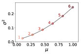
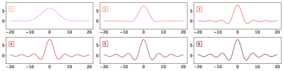
Figure 2: Top: The geodesic path between Gaussian NPSDs in the parameter space where $\sigma^{2}=\frac{\alpha}{4\pi^{2}}$ is the variance and $\mu$ is the mean. The initial NPSD has parameters $\sigma^{2}_{1}=0.025$ and $\mu_{1}=0.1$ and the final NPSD has parameters $\sigma^{2}_{2}=0.25$ and $\mu_{2}=1$. Bottom: Time-domain signals (real part) corresponding to each of the 6 PSDs in the geodesic path.

4.4 Example: data augmentation for the C. elegans dataset

The proposed interpolation method can be used for data augmentation by computing synthetic time series along the WF-interpolation path between two (real-world) signals. We next illustrate this property with the worm dataset [22], also referred to as C. elegans behavioural database [11]. Since the movements of C. elegans can be represented by combinations of four base shapes (or eigenworms) [14], a worm movement of the present dataset can be decomposed into these bases. We will only consider the class of wildtype worms on the first base shape, for which the one-dimensional time series are 900-sample long. Our aim is to construct a WF-interpolation path between the movements of two worms belonging to the same class to synthetically generate more signals having the same spectral properties.

Recall that to compute the time series from the interpolated NPSDs we need the phase, for this experiment we will interpolate the phases too in an Euclidean way: for two phases $\phi_{1}$ and $\phi_{2}$ we choose the interpolator $\phi_{\gamma}:=\gamma(\phi_{1}\operatorname{mod}2\pi)+(1-\gamma)(\phi_{2}\operatorname{mod}2\pi)$. Furthermore, we will consider an evenly-spaced frequency grid of $1001$ points between $-40$ and $40$. Fig. 3 shows a 10-step interpolation path between two C. elegans series, using the WF (top) and the Euclidean (bottom) distances.

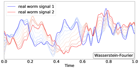
Figure 3: 10-step interpolation $(x_{\gamma})_{\gamma\in[0,1]}$ between two signals from the C. elegans database using the proposed WF distance (top) and the Euclidean distance (bottom): the true signals are shown in solid blue and red, while the interpolations are colour-coded with respect to $\gamma$.

Remark 3.

Observe that the WF interpolation is not constrained to remain in the element-wise convex hull spanned by the two series. On the contrary, under the Euclidean distance if the two series coincide in time and value, then all the interpolations are constrained to pass through that value, e.g., in Fig. 3 (bottom) for $t=0.2$ and many other time stamps.

Additionally, to assess how representative our interpolation is in the class of wildtype worms, let us refer to the distance between a NPSD $s$ and a class $C$ as

$$d(s,C)=\min_{s^{\prime}\in C}d(s,s^{\prime}),$$ (23)

and verify that the Wasserstein interpolant is closer to the wildtype class NPSDs than its Euclidean counterpart. Indeed, Fig. 4 shows our WF-interpolant (for $\gamma=0.55$) and the signal $s^{\prime}$ minimising the above distance (23) for comparison. Besides the visual similarity, notice from Table 1 that the WF interpolant is much closer to the wildtype class (using both the WF and Euclidean distances) than the Euclidean interpolant. This notion of class proximity for time series based on NPSDs opens new avenues for time series classification as we will see in Sec. 6.

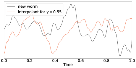
Figure 4: WF interpolant and minimiser of eq. (23): A wildtype worm signal unseen before the interpolation (black) and the proposed WF interpolant for $\gamma=0.55$ (light red).

Table 1: Class distances (in frequency domain) as defined in eq. (23) for the WF-interpolant (left) and the Euclidean interpolant (right).

	WF interpolant	Euclidean interpolant
${\mathbb{L}}_{2}$	3.9587.1e-4	$3.9905.1e-4$
$W_{2}$	0.1135	$0.2431$

4.5 Special case of Gaussian processes

The Gaussian process (GP) prior is a non-parametric generative model for continuous-time signals [39], which is defined in terms of its covariance or, via Bochner theorem (15), by its PSD. Following from the arguments in Sec. 2.1, we can identify an equivalence class of all the GPs that share the same covariance function (and hence PSD) up to a scaling constant. Identifying this equivalence class is key to extend the WF distance to GPs, which is in line with the state of the art on GPs regarding spectral covariances [57, 35, 50, 48, 51, 28, 31, 47].

The proposed interpolation is in fact a geodesic in the GP space (w.r.t. to the WF distance), where every point in the trajectory is a valid GP. The interpolation can be implemented in the space of covariance kernels simply by applying the inverse Fourier transform to the proposed WF interpolator on NPSDs, where the phase is no longer needed since covariances are even functions. In this way, as the properties of a GP are determined by its kernel (e.g., periodicity, differentiability, long-term correlations, and band-limitedness), the WF interpolant is a transition in the space of GPs with these properties. Fig. 5 illustrates this interpolation for four different covariance kernels, notice how the interpolation results on smooth incorporation of frequency components.

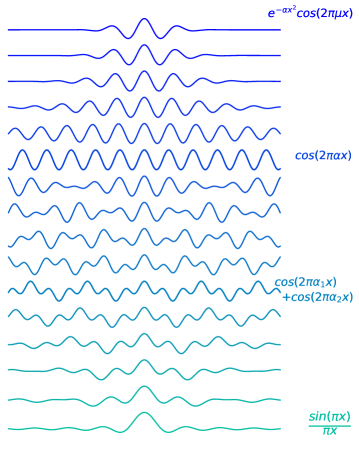
Figure 5: Interpolation of four covariance kernels colour coded: spectral mixture (blue, [57]), cosine (violet), cosine mixture (turquoise), and sinc (green). Between two given kernels, we display $4$ interpolants for $\gamma\in\{0.2,0.4,0.6,0.8\}$. Optimal transport plans $\pi^{\ast}$ were computed using POT library [24].

5 Principal geodesic analysis in WF

In order to detect spectral patterns across multiple time series, we can apply dimensionality reduction techniques to their respective NPSDs. Dimensionality reduction allows for analysing the main modes of variability of a dataset by basically finding a sequence of subspaces minimising the sum—over the data—of the norms of projection residuals. Though the de facto method for dimensionality reduction applied to functions is Functional Principal Component Analysis (FPCA) [23], applying it to NPSDs provides limited interpretation. This is because using the Euclidean distance (assumed by FPCA) directly on the NPSDs might result on principal components (PC) with negative values, which are not distributions and thus hinder interpretablity. To circumvent this challenge, the Wasserstein distance can be used to extend the classical FPCA, which takes place in the Hilbert space ${\mathbb{L}}_{2}({\mathbb{R}})$, to a Principal Geodesic Analysis (PGA), which takes place in the space of densities. In our particular setting, this will allow us to perform PGA for NPSDs in the Wasserstein space.

In a nutshell, performing PGA for probability distributions in the Wasserstein space corresponds to considering a linear space tangent to the Wasserstein one, and carrying out a standard PCA in this linear space. Then, the principal components are projected back to the Wasserstein space. This procedure is referred as Principal Geodesic Analysis (PGA). For the reader’s convenience, a review of this approach is presented in Appendix 8.3.

5.1 Implementation on NPSDs: synthetic and real-world data

The PGA procedure can be applied to the space of NPSD in order to yield a meaningful decomposition of the signals’ main oscillatory modes and to summarise the information of the series into geodesic components. The algorithm to compute PGA in the Wasserstein-Fourier space is presented in Appendix 8.4. We illustrate this application via a toy example using a dataset composed of:

• Group 1: $25$ cosine signals with random frequency $f_{i}\sim\operatorname{unif}(1,5)$ and white Gaussian noise.

• Group 2: $25$ sinc signals with random parameter $a_{i}\sim\operatorname{unif}(1,5)$ and white Gaussian noise.

Fig. 6 shows $3$ signals from each group. The cosines are colour-coded in red, while the sincs are shown in yellow. Then, Fig. 7 shows the projection locations $t_{1,n}\in[-1.52,2.51]$ of all $n=50$ NPSDs along the first geodesic component $g_{1}$. In particular, the locations of the projections $t_{1,n}$ allow for a linear separation of the groups 1 and 2 since they are respectively in the ranges $t_{1,n}\in[-0.36,2.51]$ (red-coded, cosines), and $t_{1,n}\in[-1.52,-0.75]$ (yellow-coded, sinc), meaning that the group of a new sample can be identified by assessing if its first component projection is greater or less than, say, $\bar{t}=-0.5$.

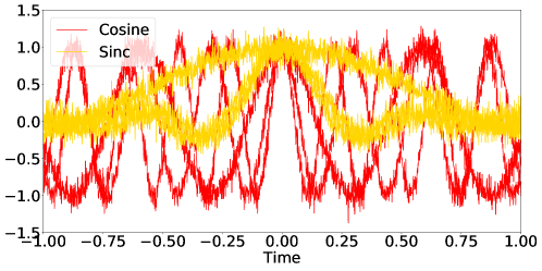
Figure 6: Subsamples of $3$ out of $25$ noisy cosine signals (red) (resp. noisy sinc signals (yellow)).

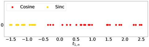
Figure 7: Values of the projection locations $(t_{1,n})_{n=1,\ldots,50}$ of the NPSDs onto the first geodesic component $g_{1}$ for the cosine (red) and sinc (yellow) signals. The groups can be linearly separated only looking at this projection.

To validate the usefulness of the proposed procedure, we also applied FPCA (i) directly on the signals, and (ii) on the NPSDs. In neither of these cases it was possible to discriminate between the sinc or cosine groups.

Lastly, we applied this decomposition procedure on the real-world fungi dataset composed of one-dimensional melt curves of the rDNA internal transcribed spacer (ITS) region of $51$ strains of $18$ fungal species ([32, 22]). Each fungi species contains between $7$ and $19$ signals, for a total of $189$ time series of length $201$. The dataset is displayed in Fig. 8, where the $18$ species are colour coded.

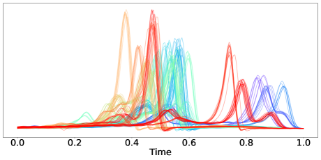
Figure 8: Melt curves for $18$ colour-coded species of fungies.

Fig. 9 shows the locations of projections $\{t_{1,n},t_{2,n}\}_{n=1}^{189}$ for the first and second components plotted against one another using the same colour-codes are the species in Fig. 8. Notice that some regions contain only projections of a single species while some species overlap (at least for the first two components), therefore, the proposed PGA might suggest that some groups have unique features isolated in different clusters while others share common properties.

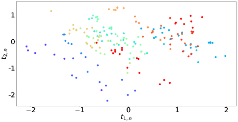
Figure 9: Values of the projection locations $(t_{1,n},t_{2,n})_{n=1,\ldots,189}$. The colours encode each fungies species, where it can be seen that some of them overlap and some do not.

6 Classification of time series using divergences

This last section is dedicated to evaluating the proposed WF distance, as well as other divergences on PSDs, as a metric for classifying time series. Note that a similar idea for a regression model has been developed in the special case of biological data in [33]. We start with a toy example motivating the use of the WF distance in the classification task, to then propose classifiers using four NPSD distances (WF, KL, IS and Euclidean) combined with the logistic function (parametric) and the $k$-nearest neighbours concept (non-parametric). Then, these classifiers are validated on binary classification using two real-world datasets.

6.1 Motivation for spectrum-based classification

Let us consider two classes of synthetic NPSDs given by

• Left-Asymetric Gaussian Mixture (L-AGM): given by a sum of two Gaussians with random means and variances, where the left Gaussian has a variance four times that of the right one.

• Right-Asymmetric Gaussian Mixture (R-AGM): constructed in the same manner but the role of the variances is reversed.

In both classes the distance between the means remains constant. Using both the Wasserstein and Euclidean metrics Fig. 10 shows samples of each class, their means or barycenters, and the distances between the samples and the means.

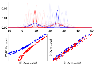
Figure 10: Illustration of the linear separability of distributions using $W_{2}$. Top: $100$ samples from each class L-AGM (light blue) and R-AGM (light red), with their Euclidean (dashed line) and Wasserstein barycenters (solid line). Bottom: Distance to the barycenter of R-AGM plotted against distance to the barycenter of L-AGM (left: Wasserstein, right: Euclidean), colour-coded by class.

Remark 4.

Only by measuring the Wasserstein distance between a sample and the class barycenters, the sample can be appropriately assigned to the corresponding class. Using the Euclidean distance, on the contrary, does not provide the required separability.

6.2 Definition of spectral classifiers for time series

We propose classifiers based on the logistic function and a $k$-nearest neighbours (KNN) classifier, both using different divergences for NPSDs as initially addressed by [38].

Table 2: Logistic Classification: Accuracy and standard error for gun shot against the 9 remaining classes of Urbansound8k. For each class, the best and second best performances are shown in boldface black and blue respectively for all KNN and logistic regression models. The last column shows the performance of $\mathcal{L}_{ALL}$ (a logistic regressor that combines ${\mathbb{L}}_{2},\operatorname{KL}$ and $W_{2}$ features) which is highlighted in red when it outperformed all 4 other single-distance logistic regressors.

	$\operatorname{KNN}_{W_{2}}$	$\operatorname{KNN}_{{\mathbb{L}}_{2}}$	$\operatorname{KNN}_{\operatorname{KL}}$	$\operatorname{KNN}_{IS}$	$\mathcal{L}_{W_{2}}$	$\mathcal{L}_{{\mathbb{L}}_{2}}$	$\mathcal{L}_{\operatorname{KL}}$	$\mathcal{L}_{IS}$	$\mathcal{L}_{ALL}$
AC	$0.734(\pm 0.065)$	$0.634(\pm 0.087)$	$0.611(\pm 0.087)$	${\color[rgb]{0,0,1}\textbf{0.769}}(\pm 0.03)$	$0.732(\pm 0.072)$	$0.718(\pm 0.047)$	$0.650(\pm 0.090)$	$\textbf{0.795}(\pm 0.036)$	$0.672(\pm 0.088)$
horn	$0.755(\pm 0.046)$	$0.783(\pm 0.037)$	$\textbf{0.809}(\pm 0.019)$	$0.681(\pm 0.042)$	$0.588(\pm 0.077)$	$0.743(\pm 0.043)$	${\color[rgb]{0,0,1}\textbf{0.790}}(\pm 0.037)$	$0.632(\pm 0.073)$	${\color[rgb]{1,0,0}\textbf{0.829}}(\pm 0.031)$
children	$0.747(\pm 0.023)$	$0.6(\pm 0.028)$	$0.672(\pm 0.014)$	$0.708(\pm 0.015)$	${\color[rgb]{0,0,1}\textbf{0.751}}(\pm 0.027)$	$0.685(\pm 0.031)$	$0.736(\pm 0.023)$	$\textbf{0.756}(\pm 0.028)$	${\color[rgb]{1,0,0}\textbf{0.769}}(\pm 0.031)$
dog bark	$0.721(\pm 0.033)$	$0.693(\pm 0.026)$	$0.658(\pm 0.028)$	$\textbf{0.746}(\pm 0.03)$	${\color[rgb]{0,0,1}\textbf{0.743}}(\pm 0.040)$	$0.720(\pm 0.033)$	$0.728(\pm 0.040)$	$0.738(\pm 0.044)$	$0.724(\pm 0.038)$
drilling	$0.82(\pm 0.019)$	$0.76(\pm 0.029)$	$0.747(\pm 0.022)$	$0.756(\pm 0.02)$	${\color[rgb]{0,0,1}\textbf{0.827}}(\pm 0.027)$	$0.826(\pm 0.026)$	$0.817(\pm 0.026)$	$\textbf{0.844}(\pm 0.023)$	$0.836(\pm 0.020)$
EI	$\textbf{0.816}(\pm 0.029)$	$0.774(\pm 0.035)$	$0.794(\pm 0.032)$	$0.791(\pm 0.038)$	$0.767(\pm 0.041)$	$0.733(\pm 0.051)$	${\color[rgb]{0,0,1}\textbf{0.791}}(\pm 0.042)$	$0.732(\pm 0.05)$	$0.791(\pm 0.045)$
J	$\textbf{0.791}(\pm 0.044)$	$0.617(\pm 0.049)$	${\color[rgb]{0,0,1}\textbf{0.737}}(\pm 0.049)$	$0.687(\pm 0.045)$	$0.645(\pm 0.087)$	$0.585(\pm 0.095)$	$0.669(\pm 0.059)$	$0.388(\pm 0.099)$	${\color[rgb]{1,0,0}\textbf{0.709}}(\pm 0.06)$
siren	$\textbf{0.924}(\pm 0.025)$	$0.868(\pm 0.038)$	$0.883(\pm 0.038)$	$0.78(\pm 0.054)$	$0.803(\pm 0.062)$	$0.878(\pm 0.034)$	${\color[rgb]{0,0,1}\textbf{0.897}}(\pm 0.034)$	$0.454(\pm 0.078)$	${\color[rgb]{1,0,0}\textbf{0.913}}(\pm 0.027)$
music	$\textbf{0.819}(\pm 0.021)$	$0.769(\pm 0.017)$	$0.763(\pm 0.023)$	${\color[rgb]{0,0,1}\textbf{0.814}}(\pm 0.028)$	$0.792(\pm 0.030)$	$0.782(\pm 0.025)$	$0.812(\pm 0.029)$	$0.284(\pm 0.67)$	${\color[rgb]{1,0,0}\textbf{0.845}}(\pm 0.028)$

Logistic classification for NPSDs. In binary classification (i.e., classes $C_{0}$ and $C_{1}$), we can parametrise the conditional probability that the sample $s$ is class $C_{1}$ using the logistic function:

$$p(C_{0}|s)=\frac{1}{1+e^{-\alpha+\beta d(s,\bar{s}_{0})-\gamma d(s,\bar{s}_{1})}},$$ (24)

where the function $d(\cdot,\cdot)$ is a divergence and $\bar{s}_{0}$ (resp. $\bar{s}_{1}$) is known as the prototype of the class $C_{0}$ (resp. $C_{1}$). For a set of sample-label observation pairs $\{(s_{i},C_{i})\}_{i=1}^{N}$, the set of parameters $[\alpha,\beta,\gamma]$ can be obtained via, e.g., maximum likelihood. Notice that, in connection with the standard (linear) logistic regression, the argument in the exponential in eq. (24) is a linear combination of the distances to class prototypes; therefore, relative proximity (on distance $d$) to the prototypes determines the class probabilities in a linear fashion.

As the sample $s$ in our setting is an NPSD, we consider four alternatives for $d$ and $\{\bar{s}_{k}\}_{k=0,1}$ in eq. (24), thus yielding four different classifiers:

1. Model $\mathcal{L}_{{\mathbb{L}}_{2}}$ : $d:={\mathbb{L}}_{2}$ the Euclidean distance, and $\bar{s}_{k}:=\frac{1}{\#C_{k}}\sum_{i\in C_{k}}x_{i}$, for $k\in\{0,1\}$, is given as the Euclidean mean of class $k$,

2. Model $\mathcal{L}_{\operatorname{KL}}$ : $d:=\operatorname{KL}$ the Kullback-Leibler distance, and $\bar{s}_{k}$ is also given as the Euclidean mean of class $k$,

3. Model $\mathcal{L}_{\operatorname{IS}}$ : $d:=\operatorname{IS}$ the Itakura-Saito distance, and $\bar{s}_{k}$ is also given as the Euclidean mean of class $k$,

4. Model $\mathcal{L}_{W_{2}}$ : $d:=W_{2}$ the Wasserstein distance, and $\bar{s}_{k}$ is given as the Wasserstein mean (26) of class $k$.

Also, as the KL and IS divergences are not symmetric, we clarify its use within models $\mathcal{L}_{\operatorname{KL}}$ and $\mathcal{L}_{\operatorname{IS}}$ via the following remark.

Remark 5.

The support of the Euclidean barycenter $\bar{s}$ of a family of distributions $\{s_{i}\}_{i}$ contains the support of each member $s_{i}$. Therefore, the KL (resp. IS) divergence computed in the following direction $\operatorname{KL}(s\|\bar{s})$ (resp. $\operatorname{IS}(s\|\bar{s})$) where $s$ is any NPSD, is always finite and thus to be considered within model $\mathcal{L}_{\operatorname{KL}}$ (resp. $\mathcal{L}_{\operatorname{IS}}$).

KNN classification for NPSDs. We also consider a variant of the KNN classifier, using the aforementioned distances on NPSDs. Recall that the KNN algorithm is a non-parametric classifier [56, 4], where sample $s$ is assigned to the class most common across its $k$ nearest neighbours. This strategy heavily relies on the distance (or divergence) used, where the predicted class follows directly from the distances among samples. Therefore, we implement the KNN concept to NPSDs using the above metrics thus yielding the classifiers $\operatorname{KNN}_{W_{2}}$, $\operatorname{KNN}_{\operatorname{KL}}$, $\operatorname{KNN}_{\operatorname{IS}}$ and $\operatorname{KNN}_{W_{2}}$. We cross-validate (on 10 folds) $k\in\{2,\cdots,10\}$ for each task and model. Results reported were obtained with the best performing $k$ for each classifier.

6.3 Binary classification of two real-world datasets

We now perform binary classification using the logistic and KNN models with the four distances (8 models in total) applied to two real-world datasets: Urbansound8k and GunPoint.

Urban audio. Urbansound8k [43] comprises 4-second recordings of the classes: air conditioner (AC), car horn, children playing, dog bark, drilling, engine idling (EI), gunshot, jackhammer (J), siren, and street music (see Table 3 in Appendix 8.5 for number of samples). We considered foreground-target recordings at 44100 Hz, that is, a dataset of 3487 one-dimensional labelled NPSDs. We focused on binary classification related to discriminating class gun shot from the remaining classes, thus having 9 different tasks.

We trained $\mathcal{L}_{W}$, $\mathcal{L}_{{\mathbb{L}}_{2}}$, $\mathcal{L}_{\operatorname{IS}}$ and $\mathcal{L}_{\operatorname{KL}}$ via maximum likelihood and cross-validated using the 10-fold as recommended by the dataset. Table 2 shows the mean accuracy of all 8 models and tasks with their 10-fold standard error, with the best and second-to-best performing methods shown in boldface black and blue respectively. Out of the nine tasks, WF is the top performer metric (through KNN) four times, and second-best performer metric (through logistic reg.) three times. Furthermore, in the three tasks where WF performed second best, its performance is well within the error bars of the top performer. Another conclusion that can be drawn is that WF seems to performs better on KNN, while IS performed better on the logistic reg. We completed our analysis with a logistic regressor that combines the features of ${\mathbb{L}}_{2},\operatorname{KL}$ and $W_{2}$ by considering a linear combination of all three distances, referred to as $\mathcal{L}_{ALL}$. This aggregated model outperformed other logistic regressors in 5 out of 9 tasks, providing an accuracy improvement of up to 0.04. This supports the idea that different features conveyed by the considered metrics can be successfully combined.

Body-motion signals. The Gunpoint dataset [40] contains hand trajectories of length $150$ from young and old actors drawing a gun or just pointing at a target with his finger. Therefore, the dataset naturally comprises two pairs of non-overlapping classes: young VS old, and drawing VS pointing. See Table 4 in Appendix 8.5 for number of samples.

For each pair of classes we performed binary classification using $10$ random splits of the dataset, using $80\%$ as training data and $20\%$ as test data. Figure 11 shows the performance in the form of box plots. Notice, for both tasks, that the top performing methods are $\operatorname{KNN}_{\operatorname{KL}}$ and $\operatorname{KNN}_{W_{2}}$ with tight error bars. For the particular case of the logistic reg. methods, $\mathcal{L}_{W_{2}}$ appears to be the best (draw VS point) and second best (young VS old) performing option. Regarding computation time, we emphasise that all distances considered belong to the same complexity class (up to a constant factor). This constant factor is relatively small (on the draw VS point task) in the logistic regression framework: $\mathcal{L}_{W_{2}}$ took 0.23 seconds to complete training in average while competing methods took 0.09 seconds. The impact of the constant factor is more visible in the $\operatorname{KNN}$ framework where WF took in average 3.7 seconds while other methods around 0.1 seconds, for the average training time.

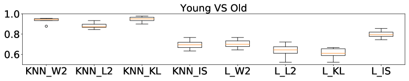
Figure 11: Classification of Gunpoint pairs: young vs old (top) and draw vs point (bottom). Accuracy and standard error using 10 different train-test ($80-20$) splits.

7 Concluding remarks

We have proposed the Wasserstein-Fourier based distance (WF) to study stationary time series. The WF distance has been presented in (i) theoretical terms, (ii) connection with consistency of the empirical autocorrelation function, (iii) data interpolation and augmentation, (iv) dimensionality reduction, and (v) time series classification. These results establish WF as a sound and intuitive metric for modern time series analysis, and thus working towards bridging the gap between the computational optimal transport and signal processing communities. The proposed WF distance is, to the best of our understanding, unique within the literature in the following aspects:

• It provides a horizontal assessment of spectral content, thus allowing to explicitly quantify the displacement of the power spectrum (frequency shift or warping). For instance, the WF distance between cosines of frequencies $\omega_{1}$ and $\omega_{2}$ is simply $|\omega_{1}-\omega_{2}|$.

• It is able to compare PSDs of different support, critically, it can compare continuous PSDs against discrete ones. For instance, it can measure the distance between a sinc function and a sum of cosines.

• It is a proper distance (unlike KL or IS) fulfilling the three axioms of a distance, and it is also meaningful from a spectral analysis perspective (unlike the Euclidean distance). This allows us translate existing distance-based methods directly to the space of time series such as dimensionality reduction, regression, classification, clustering, synthesis, or data augmentation.

In terms of computational overhead, though all distances considered are in the same order of complexity, we acknowledge that WF exhibited computation times larger than its competitors. This, however, is not detrimental for the implementation of the proposed distance, since i) WF has unique properties such as those mentioned above and therefore greater computational complexity is expected, and ii) operation on real-world examples with hundreds of time series still remained in the orders of second, both for training and prediction. Lastly, the computation of the WF distance can still be accelerated based on current developments for fast computations of the Wasserstein distance (e.g. [21]).

Future research includes exploiting the property of geodesic path between GPs, briefly illustrated in this paper, build new training procedures for Gaussian processes, as well as using optimal transport for unbalanced distributions [18], and therefore directly on the space of PSDs without the need for normalisation.

8 Appendix

8.1 Non-convexity example of the WF distance

The last equality of eq. (12) in Sec. 3.1, which serves as a counterexample for the convexity of the proposed WF distance, follows from

$$\hat{x}(\xi)=\delta(\xi-\frac{\omega}{2\pi})+\delta(\xi+\frac{\omega}{2\pi})$$

$$\widehat{y^{+}}(\xi)=\hat{x}(\xi)+\frac{1}{r}(\delta(\xi-\frac{\alpha}{2\pi})+\delta(\xi+\frac{\alpha}{2\pi}))$$

leading to

$$S_{x}(\xi)=\delta(\xi-\frac{\omega}{2\pi})+\delta(\xi+\frac{\omega}{2\pi})$$

$$S_{y^{+}}(\xi)=S_{x}(\xi)+\frac{1}{r^{2}}(\delta(\xi-\frac{\alpha}{2\pi})+\delta(\xi+\frac{\alpha}{2\pi}))$$

Normalising the PSDs, we get

$$s_{x}(\xi)=\frac{1}{2}(\delta(\xi-\frac{\omega}{2\pi})+\delta(\xi+\frac{\omega}{2\pi}))$$

$$s_{y^{+}}(\xi)=\left(\frac{r^{2}}{r^{2}+1}\right)s_{x}(\xi)+\left(\frac{1}{2(r^{2}+1)}\right)(\delta(\xi-\frac{\alpha}{2\pi})$$

$$\hskip 113.81102pt+\delta(\xi+\frac{\alpha}{2\pi})).$$

Therefore, moving the mass of $s_{y^{+}}$ onto $s_{x}$ boils down to moving the mass located in the Dirac $-\frac{\alpha}{2\pi}$ and $\frac{\alpha}{2\pi}$ onto respectively the Dirac $-\frac{\omega}{2\pi}$ and $\frac{\omega}{2\pi}$, which is twice the same cost. Therefore, we obtain

$$\operatorname{WF}\left(\left[y^{+}\right],\left[x\right]\right) =\left(\frac{2}{2(r^{2}+1)}|\frac{\omega}{2\pi}-\frac{\alpha}{2\pi}|^{2}\right)^{1/2}$$ (25)

$$=|\omega-\alpha|/(2\pi\sqrt{r^{2}+1}).$$

The derivation of $\operatorname{WF}\left(\left[y^{-}\right],\left[x\right]\right)$ works similarly.

8.2 Proof of Proposition 1

Proof.

By the normalised version of the Bochner theorem in eq. (16), and since the Fourier transform and its inverse are continuous, when $n$ tends to infinity one has that $\boldsymbol{r}_{\boldsymbol{n}}(h)\to r(h)$ is equivalent to $\boldsymbol{s}_{\boldsymbol{n}}(\xi)\to s(\xi)$, the NPSDs associated to $\boldsymbol{y}_{\boldsymbol{n}}$ and $y$. We next prove the right and left implications respectively. Note that the convergence in the Wasserstein metric is equivalent to the weak convergence and the convergence of the moments of order $p$ at the same time (see e.g. [52]).

[$\Rightarrow$] Let us assume that $\boldsymbol{s}_{\boldsymbol{n}}(\xi)\to s(\xi)$. By Scheffé’s lemma, $\boldsymbol{s}_{\boldsymbol{n}}$ weakly converges to $s$. Moreover, since $\boldsymbol{s}_{\boldsymbol{n}}$ is supported on a compact (as $y$ is band-limited), the dominated convergence theorem guarantees that $\lim_{n\to\infty}\int|\xi|^{2}{\text{d}}\boldsymbol{s}_{\boldsymbol{n}}(\xi)=\int|\xi|^{2}{\text{d}}s(\xi)$. This implies that $\lim_{n\to\infty}W_{2}(\boldsymbol{s}_{\boldsymbol{n}},s)=0$ (see e.g. Theorem 7.12 in [52]) and thus $\lim_{n\to\infty}\operatorname{WF}\left(\left[\boldsymbol{y}_{\boldsymbol{n}}\right],\left[y\right]\right)=0$.

[$\Leftarrow$] Conversely, if $W_{2}(\hat{s}_{n},s)\to 0$ when $n\to\infty$, then $\boldsymbol{s}_{\boldsymbol{n}}$ weakly converges to $s$, and by the Lévy’s continuity theorem, we have that $\lim_{n\to\infty}\int e^{jh\xi}{\text{d}}\boldsymbol{s}_{\boldsymbol{n}}(\xi)=\int e^{jh\xi}{\text{d}}s(\xi)$, which directly implies that $\lim_{n\to\infty}\boldsymbol{r}_{\boldsymbol{n}}(h)=r(h)$ for all $h$. ∎

8.3 Principal geodesic analysis: a brief review

We rely on the method proposed by [26, 36], which is next adapted to our one-dimensional setting in a simplified manner, after defining the Wasserstein mean of distributions. Let $\{s_{n}\}_{n=1}^{N}$ be a set of $N$ distributions in $\mathcal{P}_{2}({\mathbb{R}}^{d})$. A Wasserstein barycenter $\bar{s}$—or mean—of this family, is defined as the Fréchet mean with respect to the Wasserstein distance, as introduced by [1]. In other words, the Wasserstein barycenter is a solution of the following minimisation problem:

$$\bar{s}\in\operatorname*{arg\,min}_{s\in\mathcal{P}_{2}({\mathbb{R}}^{d})}\ \frac{1}{N}\sum_{n=1}^{N}W_{2}^{2}(s_{n},s).$$ (26)

The PGA procedure is then as follows:

1. For each distribution $s_{n}$, compute the projection $\ell_{n}$ onto the tangent space at the barycenter $\bar{s}$ using the logarithmic-map according to

   $$\ell_{n}=\log_{\bar{s}}(s_{n}):=F^{-}_{s_{n}}\circ F_{\bar{s}}-\operatorname{id},$$ (27)

   where recall that $F_{\bar{s}}$ denotes the cumulative function of $\bar{s}$ and $F^{-}_{s_{n}}$ the inverse cumulative function of $s_{n}$.

2. Perform FPCA on the log-map projections $\{\ell_{n}\}_{n=1}^{N}$ in the Hilbert space ${\mathbb{L}}_{2}$ weighted by the barycenter $\bar{s}$ (namely ${\mathbb{L}}_{2,\bar{s}}$), using $K$ components. Therefore, we can denote the projection of $\ell_{n}$ onto the $k\textsuperscript{th}$ component as

   $$p_{k,n}:=\hat{\ell}+t_{k,n}v_{k},$$ (28)

   where $v_{k}$ is the $k\textsuperscript{th}$ eigenvector of the log-map’s covariance matrix, $t_{k,n}$ is the location of the projection of $\ell_{n}$ onto $v_{k}$, and $\hat{\ell}$ is the Euclidean mean of $\{\ell_{n}\}_{n=1}^{N}$.

3. Map each $\{p_{k,n}\}_{k=1,n=1}^{K,N}$ back to the original distribution space using the exponential map

   $$g_{k,n}=\exp_{\bar{s}}(p_{k,n}):=(\operatorname{id}+p_{k,n})\#\bar{s},$$ (29)

   where the pusforward operator $\#$ reads for a function $T$ as $(T\#\bar{s})(A)=\bar{s}\{x\in{\mathbb{R}}^{d}|T(x)\in A\}$, for any $A\subset{\mathbb{R}}^{d}$.

Figure 12: PGA of NPSDs in the frequency domain where $\tilde{\ell}_{n}$ is the Euclidean mean of $(\ell_{n})_{n}$, $(v_{k})_{k}$ are the eigenvectors of the covariance matrix of the $\log$-maps $(\ell_{n})_{n}$ and $(t_{k,n})$ is the inner product of the $n\textsuperscript{th}\ \log$-map with the $k\textsuperscript{th}$ eigenvectors.

As a result, observe that for every pair $(k,n)$, $g_{k,n}$ is a valid distribution that corresponds to the projection of the $n\textsuperscript{th}$ original distribution $s_{n}$, onto the $k\textsuperscript{th}$ geodesic component $g_{k}$ defined by $g_{k}(t):=\exp_{\bar{s}}(\hat{\ell}+tv_{k})$, which is a distribution for each $t\in{\mathbb{R}}$. This is illustrated in Fig. 12.

Although computationally fast, the above procedure might not provide exact PGA, since a geodesic in the Wasserstein space is not exactly the image under the exponential map of straight lines in ${\mathbb{L}}_{2,\bar{s}}$ (see [12] for more details). Alternative methods are those proposed by [15] based on [12], and [34] which performs PCA on Gaussian processes by applying standard PCA on the space of covariance kernel matrices (linked to the PSDs through Bochner’s theorem).

8.4 Algorithm for PGA in Wasserstein-Fourier

The following Algorithm 1 is developed in https://github.com/GAMES-UChile/Wasserstein-Fourier.

Input: $N$ time series $(x_{n})_{i=n,\ldots,N}$
1: Compute the corresponding NPSDs $(s_{n})_{n=1,\ldots,N}$
2: Compute the quantile functions $(F^{-}_{s_{n}})_{n=1,\ldots,N}$
3: Compute the quantile of the Wasserstein barycenter $F^{-}_{\bar{s}}=\frac{1}{N}\sum_{n=1}^{N}F^{-}_{s_{n}}$ and then its cumulative function $F_{\bar{s}}$
4: For each $n=1,\ldots,N$, compute the projection $\ell_{n}=F^{-}_{s_{n}}\circ F_{\bar{s}}-\operatorname{id}$, and their Euclidean mean $\bar{\ell}=\frac{1}{N}\sum_{n=1}^{N}\ell_{n}$
5: Compute the empirical covariance operator $C\ell=\frac{1}{N}\sum_{n=1}^{N}\langle\ell_{n}-\bar{\ell},\ell\rangle_{\bar{s}}\ (\ell_{n}-\bar{\ell})$
7: Compute $(v_{k})_{1\leq k\leq K}$, the eigenvectors associated to the $K$ largest eigenvalues of $C$, and the location of the projection of $\ell_{n}$ onto $v_{k}$, namely $t_{k,n}=<\ell_{n}-\hat{\ell},v_{k}>_{\bar{s}}$
8: Construct the projections $p_{k,n}:=\hat{\ell}+t_{k,n}v_{k}$
9: Compute the geodesic principal component back into the Wasserstein space $g_{k,n}=(\operatorname{id}+p_{k,n})\#\bar{s}$

Algorithm 1 PGA in Wasserstein-Fourier

8.5 Number of samples for datasets of Section 6

class name	$\#$ samples
air conditioner	442
car horn	88
children playing	324
dog barking	367
drilling	646
engine idling	455
gun shot	132
jackhammer	408
siren	189
street music	436

Table 3: Urban sound dataset

class name	$\#$ samples
draw	100
point	100
old	215
young	236

Table 4: Body-motion dataset

References

- [1] M. Agueh and G. Carlier. Barycenters in the Wasserstein space. SIAM Journal on Mathematical Analysis, 43(2):904–924, 2011.
- [2] Shun-ichi Amari and Hiroshi Nagaoka. Methods of information geometry, volume 191. American Mathematical Soc., 2007.
- [3] L. Ambrosio, N. Gigli, and G. Savaré. Gradient flows: in metric spaces and in the space of probability measures. Springer Science & Business Media, 2008.
- [4] A. Andoni, P. Indyk, and I. Razenshteyn. Approximate nearest neighbor search in high dimensions. arXiv preprint arXiv:1806.09823, 2018.
- [5] M. Arjovsky, S. Chintala, and L. Bottou. Wasserstein generative adversarial networks. In International Conference on Machine Learning, pages 214–223, 2017.
- [6] P. Babu and P. Stoica. Spectral analysis of nonuniformly sampled data – a review. Digital Signal Processing, 20(2):359 – 378, 2010.
- [7] J. Backhoff-Veraguas, J. Fontbona, G. Rios, and F. Tobar. Bayesian learning with Wasserstein barycenters. arXiv preprint arXiv:1805.10833, 2018.
- [8] Arindam Banerjee, Srujana Merugu, Inderjit S Dhillon, and Joydeep Ghosh. Clustering with bregman divergences. Journal of machine learning research, 6(Oct):1705–1749, 2005.
- [9] Michele Basseville. Distance measures for signal processing and pattern recognition. Signal processing, 18(4):349–369, 1989.
- [10] Richard E Bellman. Adaptive control processes: a guided tour, volume 2045. Princeton university press, 2015.
- [11] Nikhil Bhatla et al. Wormweb. C. elegans, 2009.
- [12] J. Bigot, R. Gouet, T. Klein, A. López, et al. Geodesic PCA in the Wasserstein space by convex PCA. In Annales de l’Institut Henri Poincaré, Probabilités et Statistiques, volume 53, pages 1–26. Institut Henri Poincaré, 2017.
- [13] S. Bochner, M. Tenenbaum, and H. Pollard. Lectures on Fourier Integrals. Princeton University Press, 1959.
- [14] A.E. Brown, E.I. Yemini, L.J. Grundy, T. Jucikas, and W.R. Schafer. A dictionary of behavioral motifs reveals clusters of genes affecting caenorhabditis elegans locomotion. Proceedings of the National Academy of Sciences, 110(2):791–796, 2013.
- [15] E. Cazelles, V. Seguy, J. Bigot, M. Cuturi, and N. Papadakis. Geodesic PCA versus log-PCA of histograms in the Wasserstein space. SIAM Journal on Scientific Computing, 40(2):B429–B456, 2018.
- [16] C. Chatfield. The Analysis of Time Series: An Introduction. Chapman and Hall/CRC, 2016.
- [17] C. Cherry. Some experiments on the recognition of speech, with one and with two ears. The Journal of the Acoustical Society of America, 25(5):975–979, 1953.
- [18] L. Chizat, G. Peyré, B. Schmitzer, and F.X. Vialard. An interpolating distance between optimal transport and Fisher–Rao metrics. Foundations of Computational Mathematics, 18(1):1–44, 2018.
- [19] N. Choudhuri, S. Ghosal, and A. Roy. Bayesian estimation of the spectral density of a time series. Journal of the American Statistical Association, 99(468):1050–1059, 2004.
- [20] M. Cuturi and M. Blondel. Soft-DTW: a differentiable loss function for time-series. In Proceedings of the 34th International Conference on Machine Learning-Volume 70, pages 894–903. JMLR. org, 2017.
- [21] Marco Cuturi. Sinkhorn distances: Lightspeed computation of optimal transport. In C. J. C. Burges, L. Bottou, M. Welling, Z. Ghahramani, and K. Q. Weinberger, editors, Advances in Neural Information Processing Systems 26, pages 2292–2300. Curran Associates, Inc., 2013.
- [22] H.A. Dau, E. Keogh, K. Kamgar, C.M. Yeh, Y. Zhu, S. Gharghabi, C.A. Ratanamahatana, Y. Chen, B. Hu, N. Begum, A. Bagnall, A. Mueen, and G. Batista. The UCR time series classification archive. 2018.
- [23] J. Dauxois, A. Pousse, and Y. Romain. Asymptotic theory for the principal component analysis of a vector random function: some applications to statistical inference. Journal of multivariate analysis, 12(1):136–154, 1982.
- [24] R. Flamary and N. Courty. POT Python Optimal Transport library, 2017.
- [25] R. Flamary, C. Févotte, N. Courty, and V. Emiya. Optimal spectral transportation with application to music transcription. In Advances in Neural Information Processing Systems, pages 703–711, 2016.
- [26] P.T. Fletcher, C. Lu, S.M Pizer, and S. Joshi. Principal geodesic analysis for the study of nonlinear statistics of shape. IEEE transactions on medical imaging, 23(8):995–1005, 2004.
- [27] T. Henderson and J. Solomon. Audio transport: A generalized portamento via optimal transport. International Conference on Digital Audio Effects 2019 (DAFx-19), 2019.
- [28] J. Hensman, N. Durrande, and A. Solin. Variational fourier features for Gaussian processes. Journal of Machine Learning Research, 18(151):1–52, 2018.
- [29] F. Itakura. Analysis synthesis telephony based on the maximum likelihood method. In The 6th International Congress on Acoustics, pages 280–292, 1968.
- [30] S. Kay. Modern Spectral Estimation: Theory and Application. Prentice Hall, 1988.
- [31] M. Lázaro-Gredilla, J. Quiñonero Candela, C. E. Rasmussen, and A. R. Figueiras-Vidal. Sparse spectrum Gaussian process regression. Journal of Machine Learning Research, 11(Jun):1865–1881, 2010.
- [32] S. Lu, G. Mirchevska, S.S. Phatak, D. Li, J. Luka, R.A. Calderone, and W.A. Fonzi. Dynamic time warping assessment of high-resolution melt curves provides a robust metric for fungal identification. PloS one, 12(3):e0173320, 2017.
- [33] Manuel Martinez, Makarand Tapaswi, and Rainer Stiefelhagen. A closed-form gradient for the 1d earth mover’s distance for spectral deep learning on biological data. In ICML 2016 Workshop on Computational Biology (CompBio@ ICML16), 2016.
- [34] V. Masarotto, V.M. Panaretos, and Y. Zemel. Procrustes metrics on covariance operators and optimal transportation of Gaussian processes. Sankhya A, 81(1):172–213, 2019.
- [35] G. Parra and F. Tobar. Spectral mixture kernels for multi-output Gaussian processes. In Advances in Neural Information Processing Systems 30, pages 6681–6690. Curran Associates, Inc., 2017.
- [36] A. Petersen, H.G. Müller, et al. Functional data analysis for density functions by transformation to a Hilbert space. The Annals of Statistics, 44(1):183–218, 2016.
- [37] G. Peyré and M. Cuturi. Computational Optimal Transport. 2018.
- [38] A. Rakotomamonjy, A. Traore, M. Berar, R. Flamary, and N. Courty. Distance measure machines. arXiv preprint arXiv:1803.00250, 2018.
- [39] C. Rasmussen and C. Williams. Gaussian Processes for Machine Learning. The MIT Press, 2006.
- [40] C.A. Ratanamahatana and E. Keogh. Everything you know about dynamic time warping is wrong. In Third workshop on mining temporal and sequential data, volume 32. Citeseer, 2004.
- [41] A. Rolet, V. Seguy, M. Blondel, and H. Sawada. Blind source separation with optimal transport non-negative matrix factorization. EURASIP Journal on Advances in Signal Processing, 2018(1):53, 2018.
- [42] Y. Rubner, C. Tomasi, and L.J. Guibas. The earth mover’s distance as a metric for image retrieval. International Journal of Computer Vision, 40(2):99–121, 2000.
- [43] J. Salamon, C. Jacoby, and J. P. Bello. A dataset and taxonomy for urban sound research. In Proceedings of the 22nd ACM international conference on Multimedia, pages 1041–1044. ACM, 2014.
- [44] A. Schuster. On the investigation of hidden periodicities with application to a supposed 26 day period of meteorological phenomena. Terrestrial Magnetism, 3(1):13–41, 1898.
- [45] A. Takatsu. Wasserstein geometry of Gaussian measures. Osaka Journal of Mathematics, 48(4):1005–1026, 2011.
- [46] F. Tobar. Bayesian nonparametric spectral estimation. In Advances in Neural Information Processing Systems 31, pages 10148–10158, 2018.
- [47] F. Tobar. Band-limited Gaussian processes: The sinc kernel. In Advances in Neural Information Processing Systems 32, 2019.
- [48] F. Tobar, T. Bui, and R. Turner. Learning stationary time series using Gaussian processes with nonparametric kernels. In Advances in Neural Information Processing Systems 28, pages 3501–3509. Curran Associates, Inc., 2015.
- [49] R. Turner and M. Sahani. Time-frequency analysis as probabilistic inference. IEEE Transactions on Signal Processing, 62(23):6171–6183, 2014.
- [50] K. R. Ulrich, D. E. Carlson, K. Dzirasa, and L. Carin. GP kernels for cross-spectrum analysis. In Advances in Neural Information Processing Systems 28, pages 1999–2007. Curran Associates, Inc., 2015.
- [51] C. Valenzuela and F. Tobar. Low-pass filtering as Bayesian inference. In Proc. of IEEE ICASSP, pages 3367–3371, 2019.
- [52] C. Villani. Topics in Optimal Transportation. Number 58. American Mathematical Soc., 2003.
- [53] C. Villani. Optimal Transport: Old and New. Grundlehren der mathematischen Wissenschaften. Springer Berlin Heidelberg, 2008.
- [54] G. Walker. On periodicity in series of related terms. Proc. of the Royal Society of London A: Mathematical, Physical and Engineering Sciences, 131(818):518–532, 1931.
- [55] Y. Wang, R. Khardon, and P. Protopapas. Nonparametric Bayesian estimation of periodic light curves. The Astrophysical Journal, 756(1):67, 2012.
- [56] Kilian Q Weinberger and Lawrence K Saul. Distance metric learning for large margin nearest neighbor classification. Journal of Machine Learning Research, 10(Feb):207–244, 2009.
- [57] A. G. Wilson and R. P. Adams. Gaussian process kernels for pattern discovery and extrapolation. In Proc. of ICML, pages 1067–1075, 2013.
- [58] J. Ye, P. Wu, J. Z. Wang, and J. Li. Fast discrete distribution clustering using Wasserstein barycenter with sparse support. IEEE Transactions on Signal Processing, 65(9):2317–2332, 2017.
- [59] G. Udny Yule. On a method of investigating periodicities in disturbed series, with special reference to Wolfer’s sunspot numbers. Philosophical Transactions of the Royal Society of London A: Mathematical, Physical and Engineering Sciences, 226(636-646):267–298, 1927.