Zero-shot generalization using cascaded system-representations

Abstract

Behavior decompositions into primitives have been widely studied in hierarchical reinforcement learning and are known to improve generalization to changes in the environment. Conversely, does morphological decompositions into modular representations of agents lead to better generalization to changes in agent’s morphology in the same environment? In this regard, we propose a novel approach based on recurrent neural networks which learns modular representations of robots in tandem with a higher level meta-policy. We demonstrate the effectiveness of our approach by learning common control policies for a variety of analogous robots with varied kinematics and dynamics. Our emphirical results show that the policies learned using our approach can achieve performance equivalent to expert policies (policies which are trained independently for each separate robot) on previously unseen analogous robots - even with different state and action dimensionalities.

1 Introduction

(a) 2-D Reachers

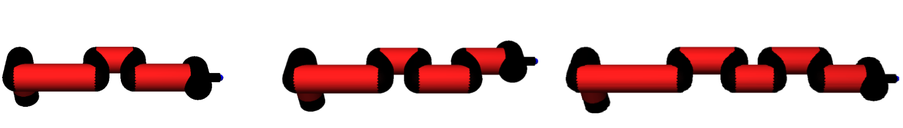
(b) Manipulators

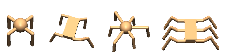
(c) Crawling robots

Figure 1: Examples of various domains of control problems for which we aim to develop a universal policy.

Deep reinforcement learning (DRL), has recently gained unprecedented success in sensorimotor control, finance, health-care, etc. However, widespread real-world adaptation of deep reinforcement learning still presents a few challenges. One of these challenges is lack of generalizability/transferability of learned policies. The performance of learned policies diminishes when properties of the agent, environment or tasks changes to regimes not encountered during training. Real world designs often do not follow a standard which raises the need to learn policies that are invariant to design choices and perform well across different operating environments. In robotics this problem manifests itself in form of morphologically different robots with vastly dissimilar hardware specifications and operational characteristics being used for similar operations (Eg. Rethink robotic’s Sawyer, Universal robotic’s UR16, etc). Currently, this necessitates the need for developing and maintaining separate hardware and morphology dependent controllers. Efforts have been made to mitigate this dependence using methods such as dynamics randomization (Peng et al., 2018) forming kernal mismatch models Rai et al. (2019) and learning variational policy embeddings Atnekvist et al. (2019) etc.. Nonetheless, learning invariant policies for different robots still remains challenging.

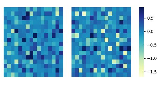
Figure 2: Abstract representations formed by the penultimate layer of networks used for training inverted pendulum agent with different seeds. Both used the same learning algorithm, hyperparameters and achieved equivalent performance.

We begin with a hypothesis that the abstract-representations learned by a neural network using conventional DRL are one of the many possible representations which could lead to similar policy performance (see fig. 2). Each of these representations entangle explanatory features required for learning optimal policy differently. The exact representations learned depend upon the network’s architecture, its initialization (Frankle & Carbin, 2018) and the learning process. Among these representations, some better capture the morphological and hardware features of robots and are thus better suited for generalizablity. Our proposed approach enforces learning of such representations. They are learned in tandem with the meta policy to ensure they are effective for the task. Better representations improves policy’s generalizability which in-turn improves quality of representations for learning policy.

Our work advances the idea proposed by Chen et al. (2018) to learn invariant policies by conditioning them on varying morphologies and hardwares. But unlike their approach which uses simple feed-forward networks, we propose a new recurrent neural architecture which we name Cascaded model network (CASNET). Our CASNET architecture is uses recurrent neural networks (RNNs) to better capture the structural features of different robots in their learned representations. The architecture is composed of 3 identifiable modules. First consists of a sequence of recurrent cells to generate morphologically dependent vector-representations. Second is a ordinary feed-forward network to learn the meta-policy and third consist of another sequence of recurrent cells to decode output of the meta-policy into actions corresponding to the robot’s morphology. CASNET is compatible with any reinforcement learning algorithm that uses temporal difference updates for state or action value functions.CASNET also provide other important advantages over Chen et al. (2018) method which we discuss ahead in the paper. Our experimental results show that universal policies which generalize over a variety of robot morphologies and hardwares can be learned using CASNET. These policies also achieve zero-shot transfer to previously unseen robots.

2 Formalization

Let $\mathbb{S}:=\{(\mathbf{s_{t}^{a}},\mathbf{s_{t}^{e}})\}$ be the joint state of the agent and its operating environment at any arbitrary time-step $t$. Agent’s observation, actions and rewards at time $t$ are $\mathbf{o}_{t}\in\mathbb{O}$, $\mathbf{a}_{t}\in\mathbb{A}$ and $r_{t}\in\mathbb{R}$, respectively. We define a degree of variation $v$ as an independent variable which is represented by an arbitrary element of $\mathbf{s_{t}^{a}}\in\mathbb{S}$, i.e., $v_{i}:=\mathbf{s_{t}^{a}}[i]$. Finally, we assume access to a set of $N$ different training environments $\bm{\varepsilon}_{\text{tr}}:=\{e^{\mathbb{D}}_{i}\}^{N}_{i=1}$ drawn from a predetermined domain $\mathbb{D}$ during training. The domain $\mathbb{D}$ is determined as:

$$\mathbb{O}^{e\sim\mathbb{D}}\subseteq\mathbb{S}\quad\big{|}\quad(\mathbf{s_{t}^{a}})_{i}\in[\min(v_{i}),\max(v_{i})]$$ (1)

Therefore, $\mathbb{D}$ is a set of all possible environments for which values of $v$ lies between specified bounds. Let $\{(\mathbf{o_{t}}^{e},\mathbf{a_{t}}^{e},r_{t}^{e})_{t=0}^{N}\}_{e\sim\bm{\varepsilon}_{\text{tr}}}$ be the data collected during training. Our goal is to use this data to formulate a predictor $P:\mathbb{O}\rightarrow\mathbb{A}$ that performs well across all $e\sim\mathbb{D}$. Emulating Ahuja et al. (2020), we achieve this objective by learning a data-representation $\Psi:\mathbb{O}\rightarrow\Upsilon\subseteq\mathbb{R}$ that elicits an invariant predictor $w\circ\Psi:\Upsilon\rightarrow\mathbb{A}$, which simultaneously maximize returns across all environments. This can be phrased as the following constraint optimization problem:

$$\underset{\Psi\in\mathbb{H}_{\Psi},w\in\mathbb{H}_{w}}{\max}\sum_{e\sim\bm{\varepsilon}_{\text{tr}}}\mathbb{E}\big{[}G^{e}(w\circ\Psi)\big{]}$$ (2)

subject to: $$w\in\text{arg }\underset{w^{\prime}\in\mathbb{H}_{w}}{\max}\mathbb{E}\big{[}G^{e}(w^{\prime}\circ\Psi)\big{]},\forall e\in\bm{\varepsilon}_{\text{tr}}$$

Here, $\mathbb{H}_{\Psi}$ and $\mathbb{H}_{w}$ are the set of all mappings $\Psi$ and predictors $w$ respectively. $G^{e}=\sum_{t=0}^{n}\gamma^{t}r_{t}$ are the returns (discounted or otherwise over finite or infinite horizon) recieved from the environment $e$. As pointed by Ahuja et al. (2020), the optimization problem 2 is difficult to solve directly and an alternate game theory based characterization can be used instead. Assume each environment has its own predictor $w^{e}\in\mathbb{H}_{w}$ and their ensemble constructs an overall predictor $\bar{w}:\Upsilon\rightarrow\mathbb{A}:=\frac{1}{|\bm{\varepsilon}_{\text{tr}}|}\sum_{j=1}^{|\bm{\varepsilon}_{\text{tr}}|}w^{j}(\psi)$, where $\psi\in\Psi$ . The new optimization problem then is:

$$\underset{\Psi\in\mathbb{H}_{\Psi},\bar{w}\in\mathbb{H}_{w}}{\max}\sum_{e\sim\bm{\varepsilon}_{\text{tr}}}\mathbb{E}\big{[}G^{e}(\bar{w}\circ\Psi)\big{]}$$ (3)

subject to: $$w^{e}\in\text{arg }\underset{w^{\prime e}\in\mathbb{H}_{w}}{\max}\mathbb{E}\Big{[}G^{e}\Big{(}(w^{\prime e}+\sum_{j\neq e}w^{j})\circ\Psi\Big{)}\Big{]},\forall e\in\bm{\varepsilon}_{\text{tr}}$$

The above constraints can be equivalently stated as a pure Nash equlibria of a game as:

$$\underset{\Psi\in\mathbb{H}_{\Psi},\bar{w}}{\max}\sum_{e\sim\bm{\varepsilon}_{\text{tr}}}\mathbb{E}\big{[}G^{e}(\bar{w}\circ\Psi)\big{]}$$ (4)

subject to: $$\mathbb{E}\Big{[}G^{e}\Big{(}\frac{1}{|\bm{\varepsilon}_{\text{tr}}|}\big{[}w^{e}+\sum_{j\neq e}w^{j}\big{]}\circ\Psi\Big{)}\Big{]}$$

$$\geq\mathbb{E}\Big{[}G^{e}\Big{(}\frac{1}{|\bm{\varepsilon}_{\text{tr}}|}\big{[}w^{\prime e}+\sum_{j\neq e}w^{j}\big{]}\circ\Psi\Big{)}\Big{]},\forall w^{\prime e}\in\mathbb{H}_{w},\forall e\in\bm{\varepsilon}_{\text{tr}}$$

This is a non-zero sum continuous game that is played between $|\bm{\varepsilon}_{\text{tr}}|$ players. Each player corresponds to $e\in\bm{\varepsilon}_{\text{tr}}$ and their set of actions are choosing $w^{e}\in\mathbb{H}_{w}$. Each player is trying to maximize its own utility function $\mathbb{E}\big{(}R^{e}(\bar{w}\circ\Psi)\big{)}$, given a representation $\Psi$. Finding Nash equilibrium for continuous games is a challenging task for which several heuristic schemes have been proposed. Yet none of them are guaranteed to compute pure or mixed equilibrium for non-zero sum games apart from some special cases. Moreover, learning a separate $w^{e}$ for each environment is in-efficient, so, we instead learn $\bar{w}$ directly. Let $\bar{w}$ be modeled with parameters $\bm{\theta}_{\bar{w}}$. During training, each player competes to move $\bar{w}$ towards $w^{e}$ (this can be understood as a modified Best response dynamics strategy Barron et al. (2010) for finding Nash equilibrium). This characterization changes 4 to:

$$\underset{\Psi\in\mathbb{H}_{\Psi},\bar{w}}{\max}\sum_{e\sim\bm{\varepsilon}_{\text{tr}}}\mathbb{E}\big{[}G^{e}(\bar{w}\circ\Psi)\big{]}$$ (5)

subject to : $$\mathbb{E}\Big{[}G^{e}\big{(}\bar{w}\circ\Psi\big{)}\Big{]}\geq\mathbb{E}\Big{[}G^{e}\big{(}\bar{w^{\prime}}\circ\Psi\big{)}\Big{]},\forall\bar{w^{\prime}}\in\mathbb{H}_{w},\forall e\in\bm{\varepsilon}_{\text{tr}}$$

Characterization 5 is mathematically and computationally more tractable compared to 4. It additionally allows us to train $\bm{\theta}_{\bar{w}}$ using heterogeneous data batches which consist of data samples generated by different environments. To satisfy the constraint in 5, the learned representation $\Psi$ should not include any features which may lead to spurious correlations to successful or unsuccessful actions for any subsets of environments. Thus, the representation learner will learn to ignore distractors in the input data when trained in tandem with the invariant predictor. Intuitively, the resulting invariant policy finds causes of successful actions across environments and thus improves generalizability.

3 Cascaded model network

Figure 3: The CASNET architecture. Here E and D stands for recurrent neural network based encoder and decoder modules respectively. The cascade of lower to higher level representations leads to learning causality.

The proposed neural architecture is shown in fig. 3. It is composed of a sequence (cascade) of encoders which are recurrent cells, a feed-forward network that acts as meta-policy and finally another sequence of recurrent cells acting as decoders. The idea behind CASNET architecture is the hypothesis that the world is inherently compositional. It can be expressed as compositions of small sets of primitive mechanisms and structures Parascandolo et al. (2018). Complexity in the real world emerges through combinations of these primitives. By extension, analogous systems are composed of analogous subsystems assembled in different configurations. These sub-systems and their specific configurations determines a system’s distinctiveness and thus its behavior. As it is evident that humans can combine simple skills to perform highly complicated tasks, it might be a useful inductive bias for the learning models to generate complex representations of higher order systems by combining representations of lower order simpler systems. A representative example of complex higher order systems being made up of simpler systems is rotary wing UAVs. They are made up of made up of various number of propellers attached at different locations w.r.t. the center of mass on the body. These propellers can have similar or different aerodynamic properties. Another example can be crawling robots which are made up of various number of legs (first order sub-system). These legs are themselves made up of different number of actuator link pairs (second order sub-system).

Input to the CASNET architecture are agent’s observations decomposed into sets of lowest order subsystem’s observations. The first RNN cell uses this input to form sets of representations of higher-order sub-systems which are then passed as input to the next RNN cell. This sequence is followed until representation of the entire agent is achieved (Representation learner in fig. 3). This representation is then augmented with any external observation such as goal or environment’s observation and passed to meta-policy’s network. Output of the meta-policy is decoded in inverse order as that of encoders using another sequence of RNNs cells to finally output action values. Input to a decoder is output of the previous decoder (or meta-policy) combined with the hidden-states of the corresponding encoder. These hidden states enhance the input to the decoder by infusing additional sub-system specific morphological information. Such decomposition along with the use of RNN cells makes CASNET’s design modular that can work with arbitrary number of subsystems and action dimensions. The CASNET architecture forces the learner to discover high-level representations that better capture the composition (structural or causal) of the agents and thus leads to better generalization results. Because of this modular design, CASNET does not assume identical dimensionality of action or observation spaces for environments sampled from the same domain. On the other hand, the dimensionality of the most primitive subsystem’s observations and actions are assumed constant across the entire domain. However, this assumption is much less restrictive than the previous one.

Objective function design. The objective function design for each environment should be normalized to be independent of the number of subsystems of any order. This normalization prevents overfitting by ensuring that the learning process is not dominated by some sub-set of training environments which have higher or lower number of subsystems than the average. Let $L^{e}$ be the normalized objective function for any $e\sim\mathbb{D}$. Then objective for training CASNET is:

$$L_{\text{casnet}}\propto\sum_{e\sim\bm{\epsilon}_{\text{tr}}}L^{e}$$ (6)

Sequence of observations and learned representations. Subsystems can have serial (actuator-link pairs in manipulators) or parallel (legs in crawling robots) configurations. Output of the RNN cells is sensitive to the sequence of the input data. Therefore, a sequencing rule should be established for parallel configurations and should be followed for the entire domain. Representations / observations of these parallel sub-systems should be augmented with configuration information (encoder specific information in fig. 3) so that the policy is aware of the exact morphology/design of the agent.

4 Experiments

We used 3 separate domains of robotics to investigate the generalization ability of our CASNET architecture: Planer reachers, crawling robots, and 3-D manipulators. Our experiments were conducted using OpenAI gym (Brockman et al., 2016) and Mujoco physics engine (Todorov et al., 2012). Overview of these domains are given ahead are discussed in details in the Appendix. DOVs and their limits for each domain is mentioned in table 1.

Table 1: DOVs for domains used in our experiments. Values are in SI units wherever applicable.

DOV	Limits
Reacher domain
DOF	[1,5]
Link-lengths	[0.07,0.17]
Crawler domain
DOF per leg	2 or 3
Num. legs	4 or 6
Legs symmetry	Bilateral/Radial/Irregular
Joint angle limits	[0.7-1.6]
Link-lengths	[0.07,0.17]
Manipulator domain
DOF	[5, 6, 7]
Link-lengths	3 $\pm$ 25$\%$
Joint damping	30 $\pm$ 25$\%$
Joint friction	10 $\pm$ 25$\%$
Actuator torque	80 $\pm$ 25$\%$

Reachers: 15 unique simulation environments were created with the goal of reaching a randomly located (but reachable) goal. There were 3 environments per DOF of which 1 was used for training and other 2 for testing.

Crawling robots: 56 unique simulation environments were created with goal to walk in the forward direction (+y axis). 46 of these 56 environments have robot designs with variations along a single DOV (apart from total number of legs) while 10 have variations along multiple DOVs. 37 environments (including all 10 with variations along multiple DOVs) were used for testing and the rest for training.

Manipulators: 270 environments were created by randomly sampling DOV values between specified limits (90 environments per DOF). 10 environments per DOF were used for testing. Each environment followed a sparse reward setting of +1 reward for reaching the goal and 0 otherwise.

We compare our proposed CASNET architecture to the following baselines:

• Expert policies: Expert policies refer to policies learned for a single environment using an appropriately sized feed forward network.

• Implicitly encoded hardware conditioned policies (HCP-I): Chen et al. (2018) showed that HCP-I can achieve state of the art performance in generalizing over a variety of robots.

4.1 Generalization experiments

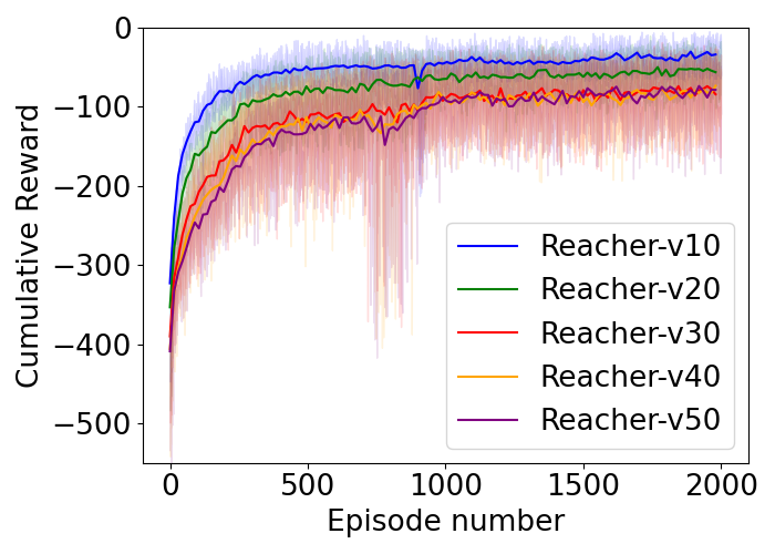
(a) CASNET Policy

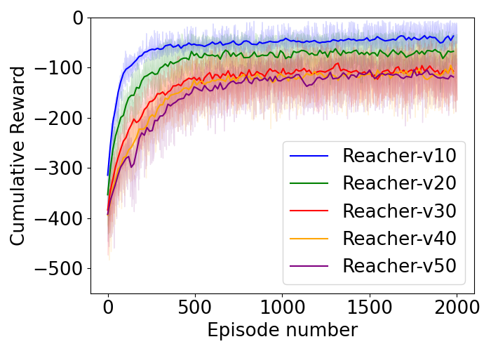
(b) Expert Policies

Figure 4: CASNET and expert policies learned for planer manipulators. Note that the expert policies are trained independently but are shown together in fig. 4(b) for facilitating comparison with the CASNET policy shown in fig. 4(a).

In this section we compare the generalization performance of out CASNET approach with baselines. Every experiment is conducted with 3 random seed value (1,2 and 3) until convergence. Hyperparameter values used are given in Appendix.

Reacher domain: Proximal policy optimization (PPO) algorithm (Schulman et al., 2017) with generalized advantage estimates (GAE) (Schulman et al., 2015) was used to train policies for Reacher domain. The CASNET agent used a single pair of encoder-decoder pair. The learning performance of CASNET policy is compared to expert policies in fig 4. Table 4 compares the final performance of CASNET policy with baselines on test environments.

Crawler robots domain: Soft actor critic (SAC) algorithm (Haarnoja et al., 2018) was used to train policies for Crawling robots. The CASNET agent used 2 encoder-decoder pairs, one for encodings and decoding leg states and other for the whole robots. Performance comparison of CASNET and baselines on test environments is summarized in table 4.

Manipulator domain: Deep deterministic policy gradient (DDPG) (Silver et al., 2014) with Hindsight experience replay (HER) (Andrychowicz et al., 2017) for training policies for manipulator domain. The CASNET architecture used is similar to the one used for Reacher domain. Table 2 compares the performance of the CASNET policy against the baselines. Nomenclature Manipulator_Yx means testing environments with Y DOFs.

Table 2: Performance comparison: Manipulator domain

Name	Success-ratio $\pm$ Standard dev.
	Expert			CASNET			HCP-I
Manipulator-v5x	0.91	$\pm$	0.14	0.84	$\pm$	0.22	0.76	$\pm$	0.20
Manipulator-v6x	0.79	$\pm$	0.17	0.83	$\pm$	0.18	0.73	$\pm$	0.20
Manipulator-v7x	0.76	$\pm$	0.18	0.67	$\pm$	0.34	0.59	$\pm$	0.25
Cumulative	0.82	$\pm$	0.18	0.78	$\pm$	0.27	0.70	$\pm$	0.23

For our selected domains, we see that CASNET regularly performs considerably better than HCP-I. It even performs better than expert policies in significant number of cases. This signifies that CASNET architecture can learn the underlying causal structures and morphological features which help in learning robust policies. The learned policies consistently perform well across the selected domain.

Table 3: Performance comparison: Reacher domain

Name	Avg. rewards $\pm$ Standard dev.
	Expert			CASNET			HCP-I
Reacher-v11	-68.1	$\pm$	3.2	-48.6	$\pm$	5.5	-62.1	$\pm$	5.5
Reacher-v12	-42.7	$\pm$	4.0	-33.5	$\pm$	2.3	-42.0	$\pm$	1.9
Reacher-v21	-72.4	$\pm$	1.5	-58.3	$\pm$	2.7	-65.1	$\pm$	3.6
Reacher-v22	-80.8	$\pm$	2.2	-65.7	$\pm$	3.3	-72.7	$\pm$	4.6
Reacher-v31	-85.0	$\pm$	3.1	-65.1	$\pm$	1.7	-77.7	$\pm$	5.4
Reacher-v32	-99.1	$\pm$	2.4	-78.6	$\pm$	4.7	-91.4	$\pm$	5.2
Reacher-v41	-102.3	$\pm$	3.0	-74.6	$\pm$	2.3	-90.5	$\pm$	4.1
Reacher-v42	-106.0	$\pm$	3.9	-75.4	$\pm$	4.0	-102.2	$\pm$	8.7
Reacher-v51	-135.8	$\pm$	4.3	-95.4	$\pm$	0.6	-116.5	$\pm$	2.6
Reacher-v52	-130.2	$\pm$	1.3	-95.1	$\pm$	2.3	-116.3	$\pm$	5.3
Cumulative	-92.2	$\pm$	27.2	-69.0	$\pm$	18.6	-83.6	$\pm$	23.5

Table 4: Performance comparison: Crawler-robots domain

Robot-type	Avg. rewards $\pm$ Standard dev.
	Expert			CASNET			HCP-I
Hexapod-v1x	961.2	$\pm$	66.1	1003.9	$\pm$	6.5	977.4	$\pm$	46.9
Hexapod-v2x	648.7	$\pm$	435.3	694.8	$\pm$	298.8	543.3	$\pm$	428.7
Hexapod-v3x	976.6	$\pm$	34.3	1006.9	$\pm$	6.5	1006.4	$\pm$	5.6
Hexapod-v4x	132.3	$\pm$	199.1	992.3	$\pm$	19.2	458.9	$\pm$	483.5
Hexapod-v5x	877.4	$\pm$	178.1	804.9	$\pm$	256.7	650.9	$\pm$	437.3
Quadruped-v1x	983.0	$\pm$	110.2	997.4	$\pm$	4.4	1002.8	$\pm$	7.7
Quadruped-v2x	417.8	$\pm$	495.5	660.3	$\pm$	247.1	599.4	$\pm$	447.9
Quadruped-v3x	287.6	$\pm$	371.2	723.2	$\pm$	420.7	693.4	$\pm$	418.6.1
Quadruped-v4x	990.2	$\pm$	34.9	1000.4	$\pm$	3.7	1007.0	$\pm$	16.5
Quadruped-v5x	807.7	$\pm$	281.9	843.2	$\pm$	203.0	879.6	$\pm$	293.4
Cumulative	720.1	$\pm$	399.0	860.5	$\pm$	250.8	774.0	$\pm$	388.8

4.2 Learned data-representations

The performance of the learned invariant policy is dependent on the quality of learned representations and how well the capture and differentiate features of different morphologies. The verify the characteristics of representations learned by CASNET’s policy, we plot them (via-dimensionality reduction) in figure 5.

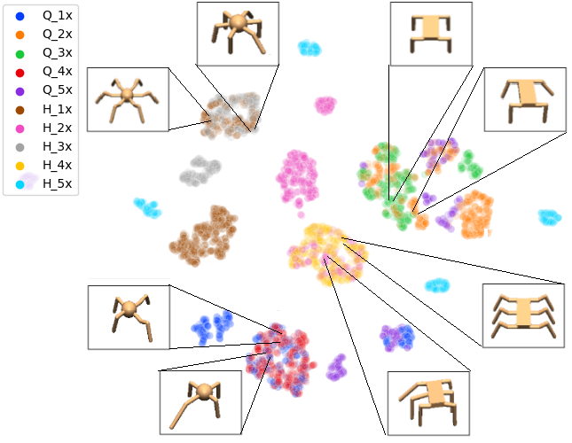
(a) Learned crawler robots representations

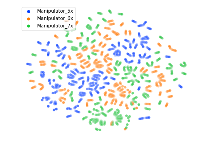
(b) Learned manipulator representations

Figure 5: t-SNE (Maaten & Hinton, 2008) visualizations of learned representations

We observe that representations form distinct clusters based upon DOVs. Representations of crawling robots with multiple DOVs are spread among representations of robots with single DOVs. Also representations of similar morphologies (ex. H_1x and H_3x) often overlap. This indicates that CASNET can also captures similarities between different morphologies which is essential for better generalization.

4.3 Out of distribution generalization and retraining

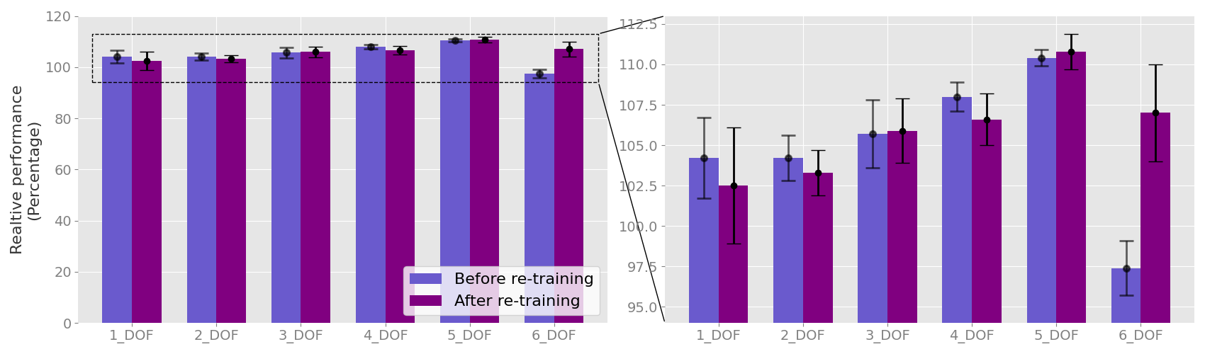
Figure 6: CASNET’s performance before and after re-training for 6-DOF reachers. Here 100 percent corresponds to average performance of expert policies while 0 percent signifies performance of random actions.

Modular structures that capture the dynamics across environments have been shown to lead to better generalization and robustness to changes Goyal et al. (2019). In this sub-section,we determine how well the CASNET agents can capture the underlying causal mechanism across environments drawn from distribution outside the training domain. Additionally, as RNNs can take inputs of arbitrary size, a trained CASNET agent should be able to scale to new input and output sizes. For robotics, these mean that a learned CASNET policy, in theory, should be extendable to new environments with relatively relaxed DOV limits than the ones used to train the agent (including environments with different actions or state dimensionalities) with no or minimal retraining. Re-training, if required, can even be performed with only new morphologies thereby alleviating the need to store the training data and/or morphologies.

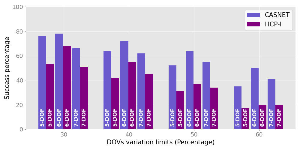
Figure 7: Performance on robots drawn from outside the training domain.

3 new Reacher environments were created with 6-DOFs each while keeping other DOV limits the same to test how well the trained CASNET agent can perform with new state and action dimensionalities. The new environments had the same observation and action space composition as the previous environments (except for the addition of a new link). The performance of the CASNET policy on these new environment before and after retraining is shown in fig. 6. The average retraining loss is 1.27% across previous environments. Re-training the agent was done using a single 6-DOF Reacher and only used 1.5% of the training data compared to training of the initial CASNET policy. The Hardware conditioned policies method cannot offer such flexibility due to its use of simple multi-layered perceptron and would thus require re-training from scratch.

To test how well the CASNET agent perform on environments drawn from out of training distribution domain DOV limits were gradually increased from 25% (limit used for training). The generalization results are shown in fig. 7. For each new DOV limit instance, 30 new environments were created and result are average of 100 episodes per DOF. The CASNET agents consistently performs considerably better than HCP-I agent with generalization performance difference increasing with increasing limits.

5 Conclusion and future works

In summary, we introduced a new neural architecture named CASNET which can learn policies that generalize to analogous environments/systems. CASNET is compatible with any temporal difference based reinforcement learning method. We tested CASNET for learning control policies for 3 different and popular domains of robotics: Planer reachers, crawling robots and 3D Manipulators using state of the art on and off-policy learning algorithms. The on-par performance of the general policies learned using CASNET with expert policies trained individually for separate robot models demonstrate that the final performance of the CASNET policies are bound by the learning algorithm instead of the proposed framework. We also tested CASNET agent’s ability to generalize to out-of-distribution data and established that the trained agent can capture the underlying causal mechanisms across different environments/robots.

6 Related Works

Transfer learning has been a major focus of the reinforcement learning and robotics community. Extensive studies have been conducted in transferring policies from simulations to the real world (Peng et al., 2018; Tobin et al., 2017; Barrett et al., 2010; Zhang et al., 2016; 2017; van Baar et al., 2019), across tasks (Fu et al., 2016; Pinto & Gupta, 2017) and dynamics (Rajeswaran et al., 2016; Mandlekar et al., 2017). However, this current work is more closely related to transferring skills amongst multiple agents. Notable works in this direction include Devin et al. (2017); Hu & Montana (2019); Gupta et al. (2017); Helwa & Schoellig (2017); Bocsi et al. (2013); Chen et al. (2018).

Bocsi et al. (2013) used transfer learning to learn dynamics models for manipulators. They used the data generated from different experiments and robot models to obtain low dimensional manifolds.Subsequently, they used their proposed algorithm to find an isomorphism between these manifolds to transfer tasks across them. Helwa & Schoellig (2017) through the study of single-input single-output systems showed that these isomorphisms are dynamic in nature. They provided an algorithm to reduce transfer learning error by determining the order and regressors of these transfer learning maps.In Gupta et al. (2017) trained invariant feature spaces using shared skills of morphologically different agents (simulated manipulators with various DOFs). These spaces were then used to share learned skill structure from one agent to others which accelerates the learning process of this skill in the latter. However, instead of facilitating the learning process across agents, our work aims to achieve zero-shot(no learning required) generalization of the learned skills. Working on a similar domain, recent work by Hu & Montana (2019) transferred acquired skills amongst morphologically different agents (MDAs). Compared to the work by Gupta et al. (2017), their experimental agents included considerably different morphologies (bipeds,single-legged hoppers, crawlers,etc.). They proposed a novel paired variational encoder-decoder to model morphology-invariant and morphology-dependent factors to expedite transfer learning. Devin et al. (2017) decomposed the policies into task and robot-specific modules. These modules were trained in a mix and match fashion for both visual and non-visual tasks. Their method achieved zero-shot generalization to novel task and robot modules combinations which were not used during the training phase. This method however required the robot and task modules to be predetermined before training the entire ensemble of modules, which prevents this method from scaling to new robot modules without significant re-training.

Among the plethora of works, CASNET is arguably most closely related to HCP-I introduced by Chen et al. (2018). They proposed Hardware conditioned policies that use hardware information to generalize the policy network over robots with different kinematics and dynamics. Robot states were augmented with either explicit or implicit encodings of robot hardware and used as input to the policy network. However, they used zero-padding to generate fixed-length state-vectors for robots with different DOFs, which restricts the learned policy’s applicability to a predetermined limit of DOFs that cannot be extended without retraining the policy from scratch. In contrast, CASNET uses RNN based encoders and decoders to generate fixed-sized representation vectors from arbitrary sized state vectors and arbitrary sized action/output vectors from fixed-sized policy output.

With CASNET, our aim is to take a meaningful step towards universal controllers which can optimally operate a plethora of different systems. Such steps have been taken for UAVs (Bulka & Nahon, 2018) and gait generation of crawling robots (Malik, 2019). However, with CASNET, we aim at providing a neural architecture for generating such controllers.

Appendix A Environment details

A.1 Planer reachers

Table 5: Reacher environments

Environment Details
Sr. No.	Name	DOFs	Link lengths
1	Reacher_10*	1	[10]
2	Reacher_11	1	[15]
3	Reacher_12	1	[09]
4	Reacher_20*	2	[12, 12]
5	Reacher_21	2	[09, 14]
6	Reacher_22	2	[13, 15]
7	Reacher_30*	3	[15, 17, 09]
8	Reacher_31	3	[08, 11, 12]
9	Reacher_32	3	[10, 10, 15]
10	Reacher_40*	4	[10, 16, 13, 09]
11	Reacher_41	4	[13, 14, 07, 07]
12	Reacher_42	4	[08, 15, 09, 11]
13	Reacher_50*	5	[10, 10, 10, 10, 10]
14	Reacher_51	5	[15, 08, 09, 11, 13]
15	Reacher_52	5	[10, 09, 12, 10, 14]
16	Reacher_60*	6	[10, 08, 15, 15, 10, 09]
17	Reacher_61	6	[08, 09, 07, 13, 14, 07]
18	Reacher_62	6	[10, 12, 08, 13, 07, 14]

Details of the 18 planer reacher environments used in experiments are shown in table 5. The environments used for training are marked with *. There are 3 environments with 1 to 6-DOFs with varying link lengths. Every actuator has the same torque limits and control range of -1 to +1 inclusive, which avoids the need to normalize actuator torque values for each environment. The state-space for each environment comprise of joint position, joint angular velocity and link-length for each actuator-link pair. The action space consist of the control values for the actuators. The objective for each environment is to reach a goal position randomly located with the robot’s reach. The reward signal at every time-step is the negative sum of the distance between the robot’s finger and the goal and squared average torque per actuator. Both these reward components are independent of the number of actuator-link pairs in reacher design. Each episode starts with reacher in fixed starting position (joint position corresponding to 0). An episode consist of 300 time-steps.

A.2 Crawling robots

Details about the crawling robot environments used in experiments are given in table 6 and table 7. The control range for each actuator is -1 to +1 inclusive. The state-space for each actuator-link pair consist of link-length, joint-range, actuator’s axis or rotation and joint-position. Coxa’s base location with respect to the center of mass (COM) of the robot is provided for each leg as encoded-specific input to the second encoder in the representation learner. Action-space consist of actuator control values. The objective for each environment is to walk in the forward direction (+y axis).The leg numbers are sequenced in clockwise fashion with respect to the z-axis (perpendicular to the surface pointing upwards). Each episode lasts 512 time-steps. At each time-step, reward is sum of movement reward, survival reward and torque-penalty. Movement rewards is propotional to COM’s speed in forward direction and survival reward is +1 for each time-step the COM is not too close or far from the surface and 0 otherwise. Torque penalty is proportional to negative root mean square value of actuator torques per number of actuators.

Table 6: Crawling robot environments. Note that L, C, F and T stand for Leg, Coxa, Femur and Tibia respectively. For example, C1 refers to the Coxa of Leg1.

Environment Details
Sr. No.	Type	Suffix	Leg symmetry	DOFs per leg	Design modifications
1	Quadruped	10*	Radial	2	None
2	Quadruped	11*	Radial	2	3-DOF in L1
3	Quadruped	12	Radial	2	3-DOF in L1, L2
4	Quadruped	13	Radial	3	2-DOF in L4
5	Quadruped	14	Radial	3	None
6	Quadruped	20	Bilateral	2	None
7	Quadruped	21*	Bilateral	2	3-DOF in L1
8	Quadruped	22*	Bilateral	2	3-DOF in L2
9	Quadruped	23	Bilateral	2	3-DOF in L3
10	Quadruped	24	Bilateral	2	3-DOF in L4
11	Quadruped	25	Bilateral	3	2-DOF in L2, L4
12	Quadruped	26*	Bilateral	3	None
13	Quadruped	31	Bilateral	2	Modified C1,T1,T4 ranges
14	Quadruped	32*	Bilateral	2	Modified C3,C4,T2 ranges
15	Quadruped	33*	Bilateral	2	Modified C1,C2,C3 ranges
16	Quadruped	34	Bilateral	2	Modified C3,C4,T4 ranges
17	Quadruped	35	Bilateral	2	Modified C2,T1,T2 ranges
18	Quadruped	41	Radial	2	Modified C1,T3,T4 lengths
19	Quadruped	42	Radial	2	Modified C2,C3,T3 lengths
20	Quadruped	43*	Radial	2	Modified C1,C2,T4 lengths
21	Quadruped	44*	Radial	2	Modified C1,T2,T4 lengths
22	Quadruped	45	Radial	2	Modified C2,C3,T1 lengths
23	Hexapod	10*	Radial	2	None
24	Hexapod	11*	Radial	2	3-DOF in L2
25	Hexapod	12	Radial	2	3-DOF in L2, L6
26	Hexapod	13	Radial	2	3-DOF in L2, L4, L6
27	Hexapod	14	Radial	3	2-DOF in L3, L5
28	Hexapod	15	Radial	3	2-DOF in L5
29	Hexapod	16*	Radial	3	None
30	Hexapod	20	Bilateral	2	None
31	Hexapod	21*	Bilateral	2	3-DOF in L1
32	Hexapod	22*	Bilateral	2	3-DOF in L1, L3
33	Hexapod	23	Bilateral	3	2-DOF in L2, L4, L6
34	Hexapod	24	Bilateral	3	2-DOF in L4, L6
35	Hexapod	25*	Bilateral	3	2-DOF in L6
36	Hexapod	26	Bilateral	3	None
37	Hexapod	31	Radial	2	Modified C1,C6,T2 ranges
38	Hexapod	32*	Radial	2	Modified C3,T3,T4 ranges
39	Hexapod	33*	Radial	2	Modified T1,T3,T5 ranges
40	Hexapod	34	Radial	2	Modified C2,C5,T6 ranges
41	Hexapod	35	Radial	2	Modified C2,T3,T4 ranges
42	Hexapod	41	Bilateral	2	Modified C1,C2,C6 lengths
43	Hexapod	42	Bilateral	2	Modified C6,T3,T5 lengths
44	Hexapod	43*	Bilateral	2	Modified C3,C4,T4 lengths
45	Hexapod	44*	Bilateral	2	Modified C5,T1,T6 lengths
46	Hexapod	45	Bilateral	2	Modified C1,T2,T5 lengths

Table 7: Crawling robot environments with multiple DOVs.

Environment Details
Sr. No.	Type	Suffix	Leg symmetry	DOFs per leg	Design modifications
1	Quadruped	51	Radial	2	- L1 base location - T1 length - C3, T4 ranges
2	Quadruped	52	Bilateral	2	- 3 DOF L3 - F3 length - C2, T1 ranges
3	Quadruped	53	Radial	3	- 2 DOF L4 - F3 length - L3, L4 base location - F1 range
4	Quadruped	54	Radial	3	- L3 base location - F1 length - T2 range
5	Quadruped	55	Radial	3	- 2 DOF L1,L3 - F4 length - C2, T1, F4 ranges
6	Hexapod	51	Radial	2	- 3 DOF L2, L6 - T2, C4 lengths - C1, F6 ranges
7	Hexapod	52	Radial	2	- 3 DOF L2 - F2 length - T5 range
8	Hexapod	53	Radial	2	- L5 base location - F2 length - C1, T1 range
9	Hexapod	54	Bilateral	3	- L4 base location - 2 DOF L2,L4,L6 - F3 length - C3, T3 range
10	Hexapod	55	Bilateral	3	- L6 base location - C3, T3 range - F2 range

Appendix B Hyperparameters

Table 8: Planer reachers

Learning algorithm	Proximal Policy Optimization
Learning rate	0.0003
Total episodes	2000
Batch size	4
Clip-range	0.2
Gamma	0.99
Lambda	0.95

Table 9: Crawling robots

Learning algorithm	Soft Actor Critic
Learning rate	0.0003
Total num-steps	200000
Batch size	256
Polyak	0.05
Gamma	0.99
Alpha	0.2

Table 10: Manipulators

Learning algorithm	Deep Deterministic Policy Gradient
Learning rate	0.0001
Total num-steps	625000
Update per episode	40
Num-steps per episode	50
Batch size	64
Polyak	0.95
Gamma	0.98
Replay_K	4

References

- Ahuja et al. (2020) Kartik Ahuja, Karthikeyan Shanmugam, Kush Varshney, and Amit Dhurandhar. Invariant risk minimization games. arXiv preprint arXiv:2002.04692, 2020.
- Andrychowicz et al. (2017) Marcin Andrychowicz, Filip Wolski, Alex Ray, Jonas Schneider, Rachel Fong, Peter Welinder, Bob McGrew, Josh Tobin, OpenAI Pieter Abbeel, and Wojciech Zaremba. Hindsight experience replay. In Advances in neural information processing systems, pp. 5048–5058, 2017.
- Atnekvist et al. (2019) Isac Atnekvist, Danica Kragic, and Johannes A Stork. Vpe: Variational policy embedding for transfer reinforcement learning. In 2019 International Conference on Robotics and Automation (ICRA), pp. 36–42. IEEE, 2019.
- Barrett et al. (2010) Samuel Barrett, Matthew E Taylor, and Peter Stone. Transfer learning for reinforcement learning on a physical robot. In Ninth International Conference on Autonomous Agents and Multiagent Systems-Adaptive Learning Agents Workshop (AAMAS-ALA), volume 1, 2010.
- Barron et al. (2010) E Barron, Rafal Goebel, and R Jensen. Best response dynamics for continuous games. Proceedings of the American Mathematical Society, 138(3):1069–1083, 2010.
- Bocsi et al. (2013) Botond Bocsi, Lehel Csató, and Jan Peters. Alignment-based transfer learning for robot models. In The 2013 international joint conference on neural networks (IJCNN), pp. 1–7. IEEE, 2013.
- Brockman et al. (2016) Greg Brockman, Vicki Cheung, Ludwig Pettersson, Jonas Schneider, John Schulman, Jie Tang, and Wojciech Zaremba. Openai gym. arXiv preprint arXiv:1606.01540, 2016.
- Bulka & Nahon (2018) Eitan Bulka and Meyer Nahon. A universal controller for unmanned aerial vehicles. In 2018 IEEE/RSJ International Conference on Intelligent Robots and Systems (IROS), pp. 4171–4176. IEEE, 2018.
- Chen et al. (2018) Tao Chen, Adithyavairavan Murali, and Abhinav Gupta. Hardware conditioned policies for multi-robot transfer learning. In Advances in Neural Information Processing Systems, pp. 9333–9344, 2018.
- Devin et al. (2017) Coline Devin, Abhishek Gupta, Trevor Darrell, Pieter Abbeel, and Sergey Levine. Learning modular neural network policies for multi-task and multi-robot transfer. In 2017 IEEE International Conference on Robotics and Automation (ICRA), pp. 2169–2176. IEEE, 2017.
- Frankle & Carbin (2018) Jonathan Frankle and Michael Carbin. The lottery ticket hypothesis: Finding sparse, trainable neural networks. arXiv preprint arXiv:1803.03635, 2018.
- Fu et al. (2016) Justin Fu, Sergey Levine, and Pieter Abbeel. One-shot learning of manipulation skills with online dynamics adaptation and neural network priors. In 2016 IEEE/RSJ International Conference on Intelligent Robots and Systems (IROS), pp. 4019–4026. IEEE, 2016.
- Goyal et al. (2019) Anirudh Goyal, Alex Lamb, Jordan Hoffmann, Shagun Sodhani, Sergey Levine, Yoshua Bengio, and Bernhard Schölkopf. Recurrent independent mechanisms. arXiv preprint arXiv:1909.10893, 2019.
- Gupta et al. (2017) Abhishek Gupta, Coline Devin, YuXuan Liu, Pieter Abbeel, and Sergey Levine. Learning invariant feature spaces to transfer skills with reinforcement learning. arXiv preprint arXiv:1703.02949, 2017.
- Haarnoja et al. (2018) Tuomas Haarnoja, Aurick Zhou, Pieter Abbeel, and Sergey Levine. Soft actor-critic: Off-policy maximum entropy deep reinforcement learning with a stochastic actor. arXiv preprint arXiv:1801.01290, 2018.
- Helwa & Schoellig (2017) Mohamed K Helwa and Angela P Schoellig. Multi-robot transfer learning: A dynamical system perspective. In 2017 IEEE/RSJ International Conference on Intelligent Robots and Systems (IROS), pp. 4702–4708. IEEE, 2017.
- Hu & Montana (2019) Yang Hu and Giovanni Montana. Skill transfer in deep reinforcement learning under morphological heterogeneity. arXiv preprint arXiv:1908.05265, 2019.
- Maaten & Hinton (2008) Laurens van der Maaten and Geoffrey Hinton. Visualizing data using t-sne. Journal of machine learning research, 9(Nov):2579–2605, 2008.
- Malik (2019) Ashish Malik. A generic decentralized gait generator architecture for statically stable motion of crawling robots. In 2019 Third IEEE International Conference on Robotic Computing (IRC), pp. 612–617. IEEE, 2019.
- Mandlekar et al. (2017) Ajay Mandlekar, Yuke Zhu, Animesh Garg, Li Fei-Fei, and Silvio Savarese. Adversarially robust policy learning: Active construction of physically-plausible perturbations. In 2017 IEEE/RSJ International Conference on Intelligent Robots and Systems (IROS), pp. 3932–3939. IEEE, 2017.
- Parascandolo et al. (2018) Giambattista Parascandolo, Niki Kilbertus, Mateo Rojas-Carulla, and Bernhard Schölkopf. Learning independent causal mechanisms. In International Conference on Machine Learning, pp. 4036–4044. PMLR, 2018.
- Peng et al. (2018) Xue Bin Peng, Marcin Andrychowicz, Wojciech Zaremba, and Pieter Abbeel. Sim-to-real transfer of robotic control with dynamics randomization. In 2018 IEEE international conference on robotics and automation (ICRA), pp. 1–8. IEEE, 2018.
- Pinto & Gupta (2017) Lerrel Pinto and Abhinav Gupta. Learning to push by grasping: Using multiple tasks for effective learning. In 2017 IEEE International Conference on Robotics and Automation (ICRA), pp. 2161–2168. IEEE, 2017.
- Rai et al. (2019) Akshara Rai, Rika Antonova, Franziska Meier, and Christopher G Atkeson. Using simulation to improve sample-efficiency of bayesian optimization for bipedal robots. J. Mach. Learn. Res., 20:49–1, 2019.
- Rajeswaran et al. (2016) Aravind Rajeswaran, Sarvjeet Ghotra, Balaraman Ravindran, and Sergey Levine. Epopt: Learning robust neural network policies using model ensembles. arXiv preprint arXiv:1610.01283, 2016.
- Schulman et al. (2015) John Schulman, Philipp Moritz, Sergey Levine, Michael Jordan, and Pieter Abbeel. High-dimensional continuous control using generalized advantage estimation. arXiv preprint arXiv:1506.02438, 2015.
- Schulman et al. (2017) John Schulman, Filip Wolski, Prafulla Dhariwal, Alec Radford, and Oleg Klimov. Proximal policy optimization algorithms. arXiv preprint arXiv:1707.06347, 2017.
- Silver et al. (2014) David Silver, Guy Lever, Nicolas Heess, Thomas Degris, Daan Wierstra, and Martin Riedmiller. Deterministic policy gradient algorithms. 2014.
- Tobin et al. (2017) Josh Tobin, Rachel Fong, Alex Ray, Jonas Schneider, Wojciech Zaremba, and Pieter Abbeel. Domain randomization for transferring deep neural networks from simulation to the real world. In 2017 IEEE/RSJ International Conference on Intelligent Robots and Systems (IROS), pp. 23–30. IEEE, 2017.
- Todorov et al. (2012) Emanuel Todorov, Tom Erez, and Yuval Tassa. Mujoco: A physics engine for model-based control. In 2012 IEEE/RSJ International Conference on Intelligent Robots and Systems, pp. 5026–5033. IEEE, 2012.
- van Baar et al. (2019) Jeroen van Baar, Alan Sullivan, Radu Cordorel, Devesh Jha, Diego Romeres, and Daniel Nikovski. Sim-to-real transfer learning using robustified controllers in robotic tasks involving complex dynamics. In 2019 International Conference on Robotics and Automation (ICRA), pp. 6001–6007. IEEE, 2019.
- Zhang et al. (2016) Fangyi Zhang, Jürgen Leitner, Michael Milford, and Peter Corke. Modular deep q networks for sim-to-real transfer of visuo-motor policies. arXiv preprint arXiv:1610.06781, 2016.
- Zhang et al. (2017) Fangyi Zhang, Jürgen Leitner, Michael Milford, and Peter Corke. Sim-to-real transfer of visuo-motor policies for reaching in clutter: Domain randomization and adaptation with modular networks. world, 7(8), 2017.