Non-Hermitian bulk-boundary correspondence and auxiliary generalized Brillouin zone theory
Abstract
We provide a systematic and self-consistent method to calculate the generalized Brillouin Zone (GBZ) analytically in one dimensional non-Hermitian systems, which helps us to understand the non-Hermitian bulk-boundary correspondence. In general, a -band non-Hermitian Hamiltonian is constituted by distinct sub-GBZs, each of which is a piecewise analytic closed loop. Based on the concept of resultant, we can show that all the analytic properties of the GBZ can be characterized by an algebraic equation, the solution of which in the complex plane is dubbed as auxiliary GBZ (aGBZ). We also provide a systematic method to obtain the GBZ from aGBZ. Two physical applications are also discussed. Our method provides an analytic approach to the spectral problem of open boundary non-Hermitian systems in the thermodynamic limit.
Introduction.—Bulk-boundary correspondence (BBC) has played a fundamental role in the development of topological band theory Hasan and Kane (2010); Qi and Zhang (2011); BERNEVIG and Hughes (2013). For example, the chiral edge state can be faithfully predicted by the Chern number. A hidden assumption of the celebrated BBC is that the bulk properties of the open boundary condition (OBC) Hamiltonian can be well approximated by the Bloch Hamiltonian with periodic boundary condition (PBC) Alase et al. (2016). However, this hidden assumption is challenged in some non-Hermitian systems recently Yao and Wang (2018); Yao et al. (2018); Song et al. (2019a, b); Kunst et al. (2018); Yokomizo and Murakami (2019); Zhang et al. ; Okuma et al. (2020); Xiong (2018); Martinez Alvarez et al. (2018); Lee and Thomale (2019); Longhi (2019a); Herviou et al. (2019); Zirnstein et al. ; Jiang et al. (2019); Longhi (2019b); Imura and Takane (2019); Helbig et al. (2019); Xiao et al. (2020); Hofmann et al. (2019); Zhang and Gong (2020); Li et al. (2019a); Torres (2019); Borgnia et al. (2020); Brzezicki and Hyart (2019); Deng and Yi (2019); Edvardsson et al. (2019); Ezawa (2019); Kunst and Dwivedi (2019); Wang et al. (2019); Kawabata et al. (2019a); Gong et al. (2018); Li et al. (2019b); Shen et al. (2018); Okuma and Sato (2019a); Jin and Song (2019); Takata and Notomi (2018); Longhi (2020); Ghatak and Das (2019a); Martinez Alvarez et al. (2018); Zeuner et al. (2015); Rudner and Levitov (2009); Lieu (2018); Brody (2014); Yi and Yang (2020). To be more precise, when the OBC Hamiltonian has non-Hermitian skin effect Yao and Wang (2018); Yao et al. (2018); Song et al. (2019a, b); Kunst et al. (2018); Yokomizo and Murakami (2019); Zhang et al. ; Okuma et al. (2020); Xiong (2018); Martinez Alvarez et al. (2018); Lee and Thomale (2019); Longhi (2019a); Herviou et al. (2019); Zirnstein et al. ; Jiang et al. (2019); Longhi (2019b); Imura and Takane (2019); Helbig et al. (2019); Xiao et al. (2020); Hofmann et al. (2019); Zhang and Gong (2020); Li et al. (2019a), the spectrum between OBC and PBC can be totally distinct Yao and Wang (2018); Yao et al. (2018); Song et al. (2019a, b); Kunst et al. (2018); Yokomizo and Murakami (2019); Zhang et al. ; Okuma et al. (2020); Xiong (2018). It has been revealed that much important information of the OBC Hamiltonian can be encoded from the generalized Brillouin zone (GBZ) Yao and Wang (2018); Yao et al. (2018); Yokomizo and Murakami (2019); Zhang et al. , which is a generalization of Brillouin Zone (BZ) under the OBC in both Hermitian and non-Hermitian systems. Although the OBC breaks the translational symmetry and the generalization of BZ seems odd, the basic idea of GBZ is to find a suitable generalized Bloch Hamiltonian (GBZ Hamiltonian) such that the boundary scattering can be regarded as a perturbation. Thus the calculation of GBZ becomes important and has drawn extensive attentions recently Lee (2016); Leykam et al. (2017); Xiong (2018); Martinez Alvarez et al. (2018); Yao and Wang (2018); Yao et al. (2018); Kunst et al. (2018); Martinez Alvarez et al. (2018); Lee and Thomale (2019); Yokomizo and Murakami (2019); Herviou et al. (2019); Zirnstein et al. ; Jiang et al. (2019); Song et al. (2019a, b); Longhi (2019b, a); Okuma et al. (2020); Zhang et al. ; Borgnia et al. (2020); Brzezicki and Hyart (2019); Deng and Yi (2019); Edvardsson et al. (2019); Ezawa (2019); Ghatak and Das (2019b); Kunst and Dwivedi (2019); Wang et al. (2019). Unfortunately, up to now, there is no universal analytical method to calculate the GBZ, and the numerical method is not only time-consuming but also unreliable due to the existence numerical errors that are extremely sensitive to the lattice size and calculation precision SM (2); Colbrook et al. (2019); Böttcher and Grudsky (2005); Reichel and Trefethen (1992). In this paper, we solve this challenging problem analytically based on the concept of auxiliary GBZ (aGBZ). We show that the GBZ of a -band Hamiltonian has distinct sub-GBZs, corresponding to the distinct bands. Each sub-GBZ is a piecewise analytic closed loop, and can be described by a common algebraic equation, namely, the aGBZ equation, which can be calculated based on the concept of resultant of polynomials Res (2019); Woody (2016); Janson (2010); SM (2). We also provide a systematic method to pick up the GBZ from aGBZ. As applications of our method, we discuss the perturbation-failure effect and the BBC in the case where each band has its respective, distinct sub-GBZ.
BBC and GBZ.—We start from the following one-dimensional (1D) Bloch Hamiltonian
| (1) |
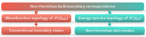
where . When , becomes Hermitian. As a result, the following discussion is also applicable for the Hermitian case. In general, Eq. 1 with OBC has two different types of nontrivial boundary states, the conventional one that has a Hermitian counterpart, and the non-Hermitian skin modes without Hermitian counterpart. Therefore, non-Hermitian Hamiltonians have two different types of BBC as shown in Fig. 1. One relates the conventional boundary state to the wavefunction topology of the GBZ Hamiltonian Yao and Wang (2018). Another relates the non-Hermitian skin modes to the (energy) spectra topology of the Bloch Hamiltonian Zhang et al. ; Okuma et al. (2020). When the spectra topology is trivial, skin modes do not exist, and GBZ coincides with BZ. As a result, the conventional boundary state can be faithfully predicted by the wavefunction topology of the Bloch Hamiltonian. Actually, the Hermitian Hamiltonian belongs to this case. However, in general, GBZ and BZ are not identical. In this case, if we want to study the boundary states protected by the wavefunction topology, the information of GBZ is necessary.
GBZ and aGBZ.—In order to characterize the non-Hermitian skin modes, we first extend the crystal momentum from real number to the entire complex plane. Since , a natural extension of Eq. 1 is
| (2) |
The eigenvalues of are determined by the following characteristic equation
| (3) |
where is the order of the pole of . For example, in the Hatano-Nelson model Hatano and Nelson (1996), it is obvious that and . Geometrically, the characteristic equation Eq. 3 defines a 2D (Riemann) surface in the 4D space . According to , each energy band (or root) corresponds to a branch of the multivalued function. When the boundary condition is fixed to PBC or OBC, the corresponding Bloch band () or GBZ band () become a set of closed loops on the Riemann surface. As shown in Fig. 2 (a) and Fig. 3 (a), the GBZ is the projection of the GBZ band on the complex -plane.
The aGBZ is defined by the projection of the following two equations on the complex -plane,
| (4) |
The mathematical meaning of aGBZ is that for a given point on it with , there must exist a conjugate point on it satisfying FN (1). Therefore, one can define the root ordering of via the following procedure: (i) solve ; (ii) order the roots by the absolute value; (iii) identify the ordering of two roots that have the same absolute value as . For example, if , then, is the root ordering of . This root ordering will be used to pick GBZ from the aGBZ. Since there exist five variables and four constraint equations , where , the solution of Eq. 4 is 1D curve in the 5D space. When the additional degrees, and , are eliminated, it can be shown that the constraint equation of the aGBZ is an algebraic equation of and ,
| (5) |
In the Supplemental Material (SM), we show how to prove Eq. 5 and calculate the coefficients by using the concept of resultant Res (2019); Woody (2016); Janson (2010); SM (2). The solid lines in Fig. 2 (b) with different colors show an example of aGBZ of the following model . Obviously, the aGBZ is constituted by a set of analytic arcs joined by the self-intersection points.
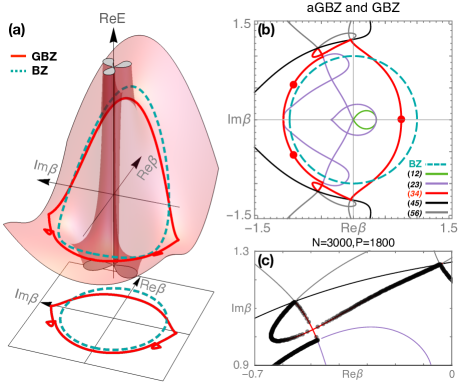
Now we show how to obtain the GBZ from aGBZ. Notice that any analytic arc on the aGBZ can be labeled by a common root ordering, as shown in Fig. 2 (b) with different colors FN (2). For the single-band models, the GBZ is constituted by all the arcs labeled by Zhang et al. ; Okuma et al. (2020), e.g., in our example. As shown in Fig. 2 (c) and SM, our analytical result is consistent with the numerical results with (lattice size) and (digit precision). However, according to the numerical result, we do not know whether there exist self-intersection points on the GBZ FN (3). We note that under the current and , the calculation time is 11 days. If we continue to improve the lattice size and numerical accuracy, the calculation time will become unacceptable. We further note that if the calculation precision is not so high (), the numerical result for may become incorrect SM (2). This is the central difficulty of the numerical calculation: the numerical diagonalization error of non-Hermitian Hamiltonians is highly sensitive to the matrix size and sometimes may lead to incorrect simulations SM (2); Colbrook et al. (2019); Böttcher and Grudsky (2005); Reichel and Trefethen (1992). Our analytical method overcomes this difficulty and can be further used to verify the accuracy of numerical calculations. On the GBZ, there exists a set of self-conjugate points satisfying , as shown in Fig. 2 (b) with red points. A statement about the self-conjugate points is that any analytic arc containing them must form the GBZ. In summary, the aGBZ is a minimal analytic element containing all the information of GBZ and the GBZ is in general a subset of aGBZ.
Generalizing the discussion to the multi-band system, we will show that the sub-GBZs for each band can be distinct. Consider the following two-band example,
| (6) |
with . The eigenvalues of the Hamiltonian are
| (7) |
where , , . As shown in Fig. 3 (a), the red and blue surfaces show the real parts of and , respectively. When the OBC is chosen, (red/blue solid lines) define two closed loop on the branches , respectively. As shown in Fig. 3 (a), their projections on the complex plane are the multi-band GBZ, which is constituted by two distinct sub-GBZs, and .
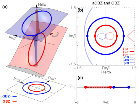
If the multi-band Hamiltonian is not block diagonal and has no additional symmetry, the GBZ is also constituted by all the arcs labeled by Yao and Wang (2018); Yokomizo and Murakami (2019); Zhang et al. ; Yi and Yang (2020), e.g., in our example with . However, if the Hamiltonian is block diagonal, e.g., in Eq. 6, then, the GBZ is the union of the ones belonging to each non-block diagonal part, namely, for in Eq. 6 FN (4). We now extract the band information from aGBZ. From the aGBZ (dashed and solid lines) shown in Fig. 3 (b), for any point on the analytic arc, Eq. 7 maps to and . By solving and ordering the roots by the absolute values, one can check which one satisfies the aGBZ condition, that is, there exist two roots having the same absolute values as . Therefore, all the analytic arcs can be further labeled by the band index. For example, the blue/red lines in Fig. 3 (b) belong to band, respectively. In our example, only the arcs with labeling constitute the GBZ. Using Eq. 7 to map to , one can obtain the GBZ spectra shown in Fig. 3 (c) with blue and red lines, which matches the numerical results (black dots) FN (5). The self-conjugate points (red and blue points) in Fig. 3 (b) and (c) correspond to the end points of the energy spectra. We finally note that each band, , can only map its own sub-GBZ, . This fact has a geometrical interpretation: each band dispersion is only defined on each branch of Eq 3.
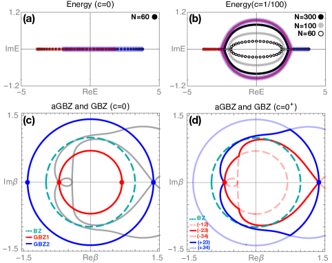
Application I: perturbation-failure.—We now show some applications of the aGBZ theory. The first one is the perturbation-failure (or critical skin) effect in non-Hermitian band theory Okuma and Sato (2019b); Li et al. (2020). As shown in Fig. 4 (a) and (b), when we choose in Eq. 6, the OBC spectrum (dots) of and exhibits a non-perturbative behavior FN (6). With the increasing of lattice size , the non-perturbative effect becomes stronger. The aGBZ theory not only provides an analytical method to understand this phenomenon, but also can strictly prove the discontinuity of the energy spectrum evolution at under the thermodynamic limit FN (7). As shown in Fig. 4 (c) and (d), when and (right-hand limit), the aGBZ of Eq. 6 are the same, namely, . However, when changes from zero to nonzero, the GBZ condition is changed. To be more precise, when , Eq. 6 is diagonal and the characteristic equation is reducible. The asymptotic solutions are determined by the two separated irreducible polynomials and , which result two independent sub-GBZs, and , as shown in Fig. 4 (c). However, when , these two bands will couple together and the GBZ is determined by the irreducible polynomial . As a result, only the arcs on the aGBZ constitute the GBZ, as shown in Fig. 4 (d). Comparing (c) and (d), it is obvious , which implies as shown by the solid lines in Fig. 4 (a) and (b), respectively.
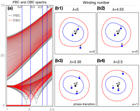
Application II: wavefunction winding number.—The second application of the aGBZ theory is the BBC in the case where each band has its respective, distinct sub-GBZ. Consider the following four-band model preserving sub-lattice symmetry Kawabata et al. (2019b),
| (8) |
where and . Since the Hamiltonian has sub-lattice symmetry, the eigenvalues come in pairs, e.g., . As a result, the sub-GBZs of and must be degenerate FN (8). Fig. 5 (a) shows the differences between OBC/PBC spectrum () as evolves. In order to characterize the emergence of topological zero modes in (a), we need to define the (wavefunction) winding number of the GBZ Hamiltonian . However, due to the existence of multiple sub-GBZs shown in Fig. 5 (b), the definition based on the matrix Yao and Wang (2018); Yokomizo and Murakami (2019) can not be extended directly FN (9). We note that once the root of passes through the GBZ, it may correspond to a topological phase transition. Therefore, it can be regarded as a topological charge. According to , the zeros can be labeled by index , which determine the sign of the charge, and band index , which is related to the sub-GBZs. When the zeros belonging to the first band () cross the sub-GBZ of second band (), as shown in Fig. 5 (b2) where the colors represent the band index, there is no gap closing and phase transition. This inspires us to write down the following conjectured formula SM (2)
| (9) |
where are the number of zeros not only satisfying but also being inside the sub-GBZ , and are the orders of the pole of . As shown in Fig. 5 (b), we plot the GBZ and the topological charges for different values of , where the black dots represent the charge of pole, namely, and ; the blue dots with charge represent the zeros belonging to the blue sub-GBZ band and satisfying . Since there are no zeros belonging to the red sub-GBZ band under the parameters shown in (b), the total winding number equals one half of the charge summation of the black dot and the blue dots inside the blue sub-GBZ. This result is consistent with Fig. 5 (a).
Discussions and conclusions.—In summary, we have provided an analytical method to calculate the GBZ, which acts as the role of the exact solution of non-Hermitian OBC Hamiltonians in the thermodynamic limit. Compared with the previous numerical methods, our work reduces the problem to the task of calculating the resultant and solving algebraic equations, the process of which is faster and error-free.
Acknowledgements.
The work is supported by the Ministry of Science and Technology of China 973 program (No. 2017YFA0303100), National Science Foundation of China (Grant No. NSFC-11888101, 1190020, 11534014, 11334012), and the Strategic Priority Research Program of CAS (Grant No.XDB07000000).References
- Hasan and Kane (2010) M. Z. Hasan and C. L. Kane, Rev. Mod. Phys. 82, 3045 (2010).
- Qi and Zhang (2011) X.-L. Qi and S.-C. Zhang, Rev. Mod. Phys. 83, 1057 (2011).
- BERNEVIG and Hughes (2013) B. A. BERNEVIG and T. L. Hughes, Topological Insulators and Topological Superconductors, stu - student edition ed. (Princeton University Press, 2013).
- Alase et al. (2016) A. Alase, E. Cobanera, G. Ortiz, and L. Viola, Phys. Rev. Lett. 117, 076804 (2016).
- Yao and Wang (2018) S. Yao and Z. Wang, Phys. Rev. Lett. 121, 086803 (2018).
- Yao et al. (2018) S. Yao, F. Song, and Z. Wang, Phys. Rev. Lett. 121, 136802 (2018).
- Song et al. (2019a) F. Song, S. Yao, and Z. Wang, Phys. Rev. Lett. 123, 170401 (2019a).
- Song et al. (2019b) F. Song, S. Yao, and Z. Wang, Phys. Rev. Lett. 123, 246801 (2019b).
- Kunst et al. (2018) F. K. Kunst, E. Edvardsson, J. C. Budich, and E. J. Bergholtz, Phys. Rev. Lett. 121, 026808 (2018).
- Yokomizo and Murakami (2019) K. Yokomizo and S. Murakami, Phys. Rev. Lett. 123, 066404 (2019).
- (11) K. Zhang, Z. Yang, and C. Fang, arXiv:1910.01131 .
- Okuma et al. (2020) N. Okuma, K. Kawabata, K. Shiozaki, and M. Sato, Phys. Rev. Lett. 124, 086801 (2020).
- Xiong (2018) Y. Xiong, J. Phys. Commun. 2, 035043 (2018).
- Martinez Alvarez et al. (2018) V. M. Martinez Alvarez, J. E. Barrios Vargas, and L. E. F. Foa Torres, Phys. Rev. B 97, 121401 (2018).
- Lee and Thomale (2019) C. H. Lee and R. Thomale, Phys. Rev. B 99, 201103 (2019).
- Longhi (2019a) S. Longhi, Opt. Lett. 44, 5804 (2019a).
- Herviou et al. (2019) L. Herviou, J. H. Bardarson, and N. Regnault, Phys. Rev. A 99, 052118 (2019).
- (18) H.-G. Zirnstein, G. Refael, and B. Rosenow, arXiv:1901.11241 .
- Jiang et al. (2019) H. Jiang, L.-J. Lang, C. Yang, S.-L. Zhu, and S. Chen, Phys. Rev. B 100, 054301 (2019).
- Longhi (2019b) S. Longhi, Phys. Rev. Research 1, 023013 (2019b).
- Imura and Takane (2019) K.-I. Imura and Y. Takane, Phys. Rev. B 100, 165430 (2019).
- Helbig et al. (2019) T. Helbig, T. Hofmann, S. Imhof, M. Abdelghany, T. Kiessling, L. W. Molenkamp, C. H. Lee, A. Szameit, M. Greiter, and R. Thomale, “Observation of bulk boundary correspondence breakdown in topolectrical circuits,” (2019), arXiv:1907.11562 .
- Xiao et al. (2020) L. Xiao, T. Deng, K. Wang, G. Zhu, Z. Wang, W. Yi, and P. Xue, Nature Physics (2020).
- Hofmann et al. (2019) T. Hofmann, T. Helbig, F. Schindler, N. Salgo, M. Brzezińska, M. Greiter, T. Kiessling, D. Wolf, A. Vollhardt, A. Kabaši, C. H. Lee, A. Bilušić, R. Thomale, and T. Neupert, (2019), arXiv:1908.02759 .
- Zhang and Gong (2020) X. Zhang and J. Gong, Phys. Rev. B 101, 045415 (2020).
- Li et al. (2019a) L. Li, C. H. Lee, and J. Gong, (2019a), arXiv:1910.03229 .
- Torres (2019) L. E. F. F. Torres, Journal of Physics: Materials 3, 014002 (2019).
- Borgnia et al. (2020) D. S. Borgnia, A. J. Kruchkov, and R.-J. Slager, Phys. Rev. Lett. 124, 056802 (2020).
- Brzezicki and Hyart (2019) W. Brzezicki and T. Hyart, Phys. Rev. B 100, 161105 (2019).
- Deng and Yi (2019) T.-S. Deng and W. Yi, Phys. Rev. B 100, 035102 (2019).
- Edvardsson et al. (2019) E. Edvardsson, F. K. Kunst, and E. J. Bergholtz, Phys. Rev. B 99, 081302 (2019).
- Ezawa (2019) M. Ezawa, Phys. Rev. B 99, 121411 (2019).
- Kunst and Dwivedi (2019) F. K. Kunst and V. Dwivedi, Phys. Rev. B 99, 245116 (2019).
- Wang et al. (2019) H. Wang, J. Ruan, and H. Zhang, Phys. Rev. B 99, 075130 (2019).
- Kawabata et al. (2019a) K. Kawabata, K. Shiozaki, M. Ueda, and M. Sato, Phys. Rev. X 9, 041015 (2019a).
- Gong et al. (2018) Z. Gong, Y. Ashida, K. Kawabata, K. Takasan, S. Higashikawa, and M. Ueda, Phys. Rev. X 8, 031079 (2018).
- Li et al. (2019b) L. Li, C. H. Lee, and J. Gong, Phys. Rev. B 100, 075403 (2019b).
- Shen et al. (2018) H. Shen, B. Zhen, and L. Fu, Phys. Rev. Lett. 120, 146402 (2018).
- Okuma and Sato (2019a) N. Okuma and M. Sato, Phys. Rev. Lett. 123, 097701 (2019a).
- Jin and Song (2019) L. Jin and Z. Song, Phys. Rev. B 99, 081103 (2019).
- Takata and Notomi (2018) K. Takata and M. Notomi, Phys. Rev. Lett. 121, 213902 (2018).
- Longhi (2020) S. Longhi, Phys. Rev. Lett. 124, 066602 (2020).
- Ghatak and Das (2019a) A. Ghatak and T. Das, Journal of Physics Condensed Matter 31 (2019a), 10.1088/1361-648X/ab11b3, arXiv:1902.07972 .
- Martinez Alvarez et al. (2018) V. M. Martinez Alvarez, J. E. Barrios Vargas, M. Berdakin, and L. E. F. Foa Torres, The European Physical Journal Special Topics 227, 1295 (2018), arXiv:1805.08200 .
- Zeuner et al. (2015) J. M. Zeuner, M. C. Rechtsman, Y. Plotnik, Y. Lumer, S. Nolte, M. S. Rudner, M. Segev, and A. Szameit, Phys. Rev. Lett. 115, 040402 (2015).
- Rudner and Levitov (2009) M. S. Rudner and L. S. Levitov, Phys. Rev. Lett. 102, 065703 (2009).
- Lieu (2018) S. Lieu, Phys. Rev. B 97, 045106 (2018).
- Brody (2014) D. C. Brody, Journal of Physics A: Mathematical and Theoretical 47 (2014), 10.1088/1751-8113/47/3/035305, arXiv:1308.2609 .
- Yi and Yang (2020) Y. Yi and Z. Yang, arXiv e-prints , arXiv:2003.02219 (2020), arXiv:2003.02219 [cond-mat.mes-hall] .
- Lee (2016) T. E. Lee, Phys. Rev. Lett. 116, 133903 (2016).
- Leykam et al. (2017) D. Leykam, K. Y. Bliokh, C. Huang, Y. D. Chong, and F. Nori, Phys. Rev. Lett. 118, 040401 (2017).
- Martinez Alvarez et al. (2018) V. M. Martinez Alvarez, J. E. Barrios Vargas, M. Berdakin, and L. E. F. Foa Torres, Eur. Phys. J. Spec. Top. 227, 1295 (2018).
- Ghatak and Das (2019b) A. Ghatak and T. Das, J. Phys.: Condens. Matter 31, 263001 (2019b).
- SM (2) See Supplemental Material for details .
- Colbrook et al. (2019) M. J. Colbrook, B. Roman, and A. C. Hansen, Phys. Rev. Lett. 122, 250201 (2019).
- Böttcher and Grudsky (2005) A. Böttcher and S. M. Grudsky, Spectral properties of banded Toeplitz matrices, Vol. 96 (Siam, 2005).
- Reichel and Trefethen (1992) L. Reichel and L. N. Trefethen, Linear Algebra and its Applications 162-164, 153 (1992).
- Res (2019) Wikipedia (2019), page Version ID: 905762282.
- Woody (2016) H. Woody, Polynomial Resultants , 10 (2016).
- Janson (2010) S. Janson, RESULTANT AND DISCRIMINANT OF POLYNOMIALS , 18 (2010).
- Hatano and Nelson (1996) N. Hatano and D. R. Nelson, Phys. Rev. Lett. 77, 570 (1996).
- FN (1) In general, and are different points on the aGBZ .
- FN (2) The reason is that for any point on the analytic arcs, the root ordering can only be changed at the self-intersection points .
- FN (3) We note that this kind of self-intersection point is a new type of singularity point, which has no counterpart in Hermitian systems and is unique to non-Hermitian systems. The details have been discussed in the SM .
- FN (4) It can be shown that and for the parameters we chosen, i.e., . .
- FN (5) We note that can only be mapped by and the corresponding GBZ spectra for band becomes . While the GBZ spectra for band becomes .
- Okuma and Sato (2019b) N. Okuma and M. Sato, Phys. Rev. Lett. 123, 097701 (2019b).
- Li et al. (2020) L. Li, C. H. Lee, S. Mu, and J. Gong, (2020), arXiv:2003.03039 .
- FN (6) This means the spectra change is lager than the perturbation strength .
- FN (7) We note that the GBZ and the corresponding GBZ spectra are defined in the thermodynamic limit .
- Kawabata et al. (2019b) K. Kawabata, K. Shiozaki, M. Ueda, and M. Sato, Phys. Rev. X 9, 041015 (2019b).
- FN (8) This is because the characteristic equation of the non-Bloch Hamiltonian preserving sub-lattice symmetry satisfies Yi and Yang (2020) .
- FN (9) The reason is that the Q matrix is defined on all occupied bands, it is not clear which sub-GBZs should be chosen as the integration path. In the SM, we provide a detailed discussion .
See pages 1 of SM.pdf See pages 2 of SM.pdf See pages 3 of SM.pdf See pages 4 of SM.pdf See pages 5 of SM.pdf See pages 6 of SM.pdf See pages 7 of SM.pdf See pages 8 of SM.pdf See pages 9 of SM.pdf See pages 10 of SM.pdf See pages 11 of SM.pdf See pages 12 of SM.pdf See pages 13 of SM.pdf See pages 14 of SM.pdf See pages 15 of SM.pdf See pages 16 of SM.pdf