Chemical properties of two dense cores in a Planck Galactic Cold Clump G168.72-15.48

Abstract

To deepen our understanding of the chemical properties of the Planck Galactic Cold Clump (PGCC) G168.72-15.48, we performed observations of nine molecular species, namely, c-C3H, H2CO, HC5N, HC7N, SO, CCH, N2H+, CH3OH, and CH3CCH, toward two dense cores in PGCC G168.72-15.48 using the Tianma Radio Telescope and Purple Mountain Observatory Telescope. We detected c-C3H, H2CO, HC5N, N2H+, CCH, and CH3OH in both G168-H1 and G168-H2 cores, whereas HC7N and CH3CCH were detected only in G168-H1 and SO was detected only in G168-H2. Mapping observations reveal that the CCH, N2H+, CH3OH, and CH3CCH emissions are well coupled with the dust emission in G168-H1. Additionally, N2H+ exhibits an exceptionally weak emission in the denser and more evolved G168-H2 core, which may be attributed to the N2H+ depletion. We suggest that the N2H+ depletion in G168-H2 is dominated by N2 depletion, rather than the destruction by CO. The local thermodynamic equilibrium calculations indicate that the carbon-chain molecules of CCH, HC5N, HC7N, and CH3CCH are more abundant in the younger G168-H1 core. We found that starless core G168-H1 may have the properties of cold dark clouds based on its abundances of carbon-chain molecules. While, the prestellar core G168-H2 exhibits lower carbon-chain molecular abundances than the general cold dark clouds. With our gas-grain astrochemical model calculations, we attribute the observed chemical differences between G168-H1 and G168-H2 to their different gas densities and different evolutionary stages.

=200

1 Introduction

Planck Galactic Cold Clumps (PGCCs) have been considered as good targets for investigating the early stage of star formation. Many observations have been conducted to understand the properties of PGCCs (Liu, Wu & Zhang, 2012; Meng, Wu & Liu, 2013; Zhang et al., 2016; Wu et al., 2012; Liu et al., 2014, 2018). For example, L1495, a filamentary cloud harboring active low-mass star forming regions, contains 16 PGCCs (Planck Collaboration et al., 2016). Recent observations of 16 PGCCs by Tang et al. (2018) identified 30 dense cores in L1495, and classified these dense cores into three groups: starless, prestellar, and protostellar cores. G168.72-15.48 (hereafter denoted as G168) is one of the 16 PGCCs detected in L1495. Figure 1 presents the spatial distributions of the dust temperature and H2 column density derived from the Herschel continuum imaging data of G168. As seen from Figure 1, there are two dense cores, G168-H1 and G168-H2. A protostellar core IRAS 04155+2812 (marked with a white cross in Figure 1) located south of G168-H2 is believed to be heating G168-H2 (Ward-Thompson et al., 2016). Dapp & Basu (2009) proposed an H2 density profile to model spherical and flattened clouds, which is characterized by a flat region ($a_{d}$), central column density ($N_{\rm c}$), central volume density ($n_{\rm c}$), and truncated radius ($R_{\rm d}$). The fitting H2 density profiles to the 30 dense cores are summarized in Table 1. As shown in Table 1, the density profile parameters ($a_{\rm d}$, $N_{\rm c}$, $n_{\rm c}$) of G168-H1 and G168-H2 correspond to the statistical results of starless core and prestellar core, respectively. Therefore, Tang et al. (2018) classified G168-H1 as a starless core and G168-H2 as a prestellar core. Starless cores will become prestellar cores when they are dense enough to be gravitationally bound. Then, the prestellar cores can collapse to form protostars (Ward-Thompson et al., 1994; Caselli, 2011). Under this sketch, G168-H2 is more evolved than G168-H1 during the earliest stage of star formation.

Considering their different evolutionary stages, G168-H1 and G168-H2 are good targets for studying properties of starless and prestellar cores. Previous observations toward G168 by Tang et al. (2018) mainly focused on the physical properties, demonstrating that G168-H1 and G168-H2 have source sizes of $394^{\prime\prime}\times 158^{\prime\prime}$ (P.A.=$-6^{\circ}$) and $251^{\prime\prime}\times 169^{\prime\prime}$ (P.A.=$-85^{\circ}$) on the angular scale, corresponding to geometric mean core radii of 0.17($\pm$0.03) and 0.14($\pm$0.02) pc at a distance of 140 pc, respectively. Volume densities of 1.89($\pm$0.21)$\times 10^{4}$ and 4.78($\pm$0.71)$\times 10^{4}$ cm^-3, dust temperatures of 11.90($\pm$0.31) and 13.25($\pm$1.02) K, and core masses of 26.47($\pm$3.04) and 37.79($\pm$5.51) M_☉ were also reported for G168-H1 and G168-H2, respectively (see Table 1). However, the chemical properties of these dense cores in G168 have not been well investigated. In this study, we investigated these two cores to deepen our understanding of the chemical properties of starless and prestellar cores in G168.

In cold dark clouds, carbon-chain and nitrogen-bearing molecules can be easily detected and are generally used for probing the properties of cold dark clouds (Benson & Myers, 1983; Benson, Caselli & Myers, 1998; Suzuki et al., 1992; Scappini & Codella, 1996; Tafalla et al., 1998; Aikawa et al., 2001; Hirota & Maezawa, 2014; Sakai et al., 2008, 2010; Suzuki, Ohishi & Hirota, 2014; Taniguchi et al., 2018). PGCCs are mainly embedded in dense regions within cold dark clouds (Planck Collaboration et al., 2016). Therefore, nitrogen-bearing and carbon-chain molecules are effective for revealing the chemical properties of PGCCs. In this paper, we present the observations of nine molecular species, namely, HC5N, HC7N, c-C3H, H2CO, SO, CCH, N2H+, CH3CCH, and CH3OH, to investigate the chemical properties of two dense cores in G168, through the observations by use of the Purple Mountain Observatory (PMO) 13.7 m telescope and TianMa 65 m Radio Telescope (TMRT).

Table 1: Parameters of G168-H1 and G168-H2

Source	Angle size	Radius	$N_{\rm H2}$	$T_{\rm d}$	$n_{\rm H2}$	Mass	$X_{\rm C^{18}O}$	$a_{\rm d}$(a)	$N_{\rm c}$(a)	$n_{\rm c}$(a)
	($\prime\prime\times\prime\prime$)	(pc)	(1022 cm-2)	(K)	(104 cm-3)	(M☉)	(10-7)	(pc)	(1022 cm-2)	(104 cm-3)
G168-H1	394$\times$158	0.17($\pm$0.03)	1.40($\pm$0.21)	11.90($\pm$0.31)	1.89($\pm$0.21)	26.47($\pm$3.04)	1.26($\pm$0.21)	0.047($\pm$0.017)	2.10($\pm$0.01)	4.65($\pm$1.75)
G168-H2	251$\times$169	0.14($\pm$0.02)	2.46($\pm$0.62)	13.25($\pm$1.02)	4.78($\pm$0.71)	37.79($\pm$5.51)	0.91($\pm$0.29)	0.025($\pm$0.001)	4.50($\pm$0.01)	17.74($\pm$1.3)
Starless
Mean	…	0.15($\pm$0.06)	0.86($\pm$0.27)	12.11($\pm$0.41)	1.47($\pm$0.53)	15.90($\pm$15.21)	1.57($\pm$0.65)	0.048($\pm$0.006)	1.27($\pm$0.11)	3.50($\pm$0.55)
Median	…	0.12($\pm$0.04)	0.86($\pm$0.26)	11.13($\pm$0.41)	1.57($\pm$0.47)	7.73($\pm$1.40)	1.61($\pm$0.34)	0.047($\pm$0.004)	1.2($\pm$0.08)	3.11($\pm$0.35)
Prestellar
Mean	…	0.10($\pm$0.03)	1.47($\pm$0.46)	11.62($\pm$0.81)	3.96($\pm$1.05)	12.9($\pm$11.40)	0.81($\pm$0.13)	0.026($\pm$0.001)	2.49($\pm$0.02)	10.33($\pm$0.68)
Median	…	0.10($\pm$0.02)	1.29($\pm$0.25)	12.13($\pm$0.33)	4.43($\pm$0.94)	8.63($\pm$1.30)	0.84($\pm$0.11)	0.025($\pm$0.001)	2.10($\pm$0.01)	9.76($\pm$0.58)

Note. — (a): $a_{\rm d}$, $N_{\rm c}$, and $n_{\rm c}$ are flat region, central column density, and central volume density respectively. They were derived from the column density profile fitting toward the dense cores of L1495 dark cloud by Tang et al. (2018).

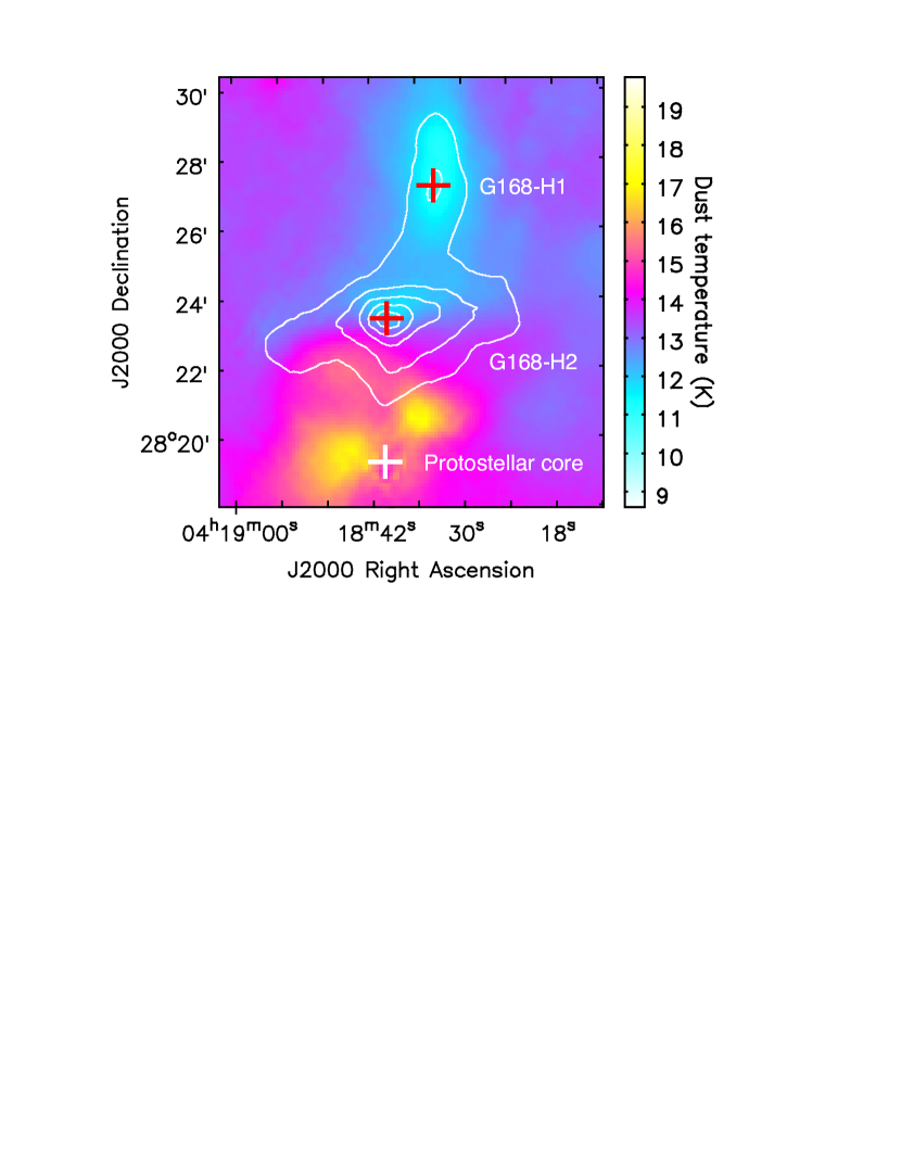
Figure 1: Herschel H2 column density map (white contours) overlaid on the Herschel dust temperature map (color). White contours range from 30% to 90%, with a step of 15% of peak value ($4.48\times 10^{22}$ cm^-2). Red crosses represent the peak positions of the G168-H1 and G168-H2 cores. White cross denotes a point source IRAS 04155+2812 (Ward-Thompson et al., 2016).

2 Observations

2.1 TMRT Observations

We performed single-pointing observations toward the G168-H1 and G168-H2 cores in the Ku band (11.5–18.5 GHz) in August 2018 with the Tianma 65 m Radio Telescope (TMRT) of Shanghai Astronomical Observatory. The observations were conducted in the position-switching mode. The digital backend system (DIBAS) of TMRT supports several observing modes (Bussa & VEGAS devolepment team, 2012). We adopted mode 20 for Ku band observations, which has a 187.5 MHz bandwidth with 32,768 channels, providing a spectral resolution of 5.722 KHz (corresponding to a velocity resolution of 0.12 km s^-1) at the Ku band. DIBAS supports two banks (A and B) for observing different frequency ranges simultaneously. In our observations, the frequency ranges of bank A and B were set at 13–14 GHz and 14–15 GHz, respectively. The transitions of HC5N(5-4), HC7N(11-10), HC7N(12-11), and SO(1₂-1₁) were tuned in bank A, and the transitions of c-C3H(J=$\frac{1}{2}$-$\frac{3}{2}$), c-C3H(J=$\frac{3}{2}$-$\frac{3}{2}$), H2CO(2_1,1-2_1,2), and HC7N(13-12) were tuned in bank B. An integrated time of 100 minutes on-source yielded a root-mean-square (rms) noise level of 20 mK for bank A. However, bank B was not stable enough during our observations, resulting in a higher rms noise level of 80 mK. The beam size of TMRT ranges from 73^′′ to 54^′′ at the frequency range of 13–18 GHz. The average beam size is 69^′′, corresponding to a linear scale of $\sim$0.05 pc at a distance of 140 pc. The main beam efficiency is 60% at the Ku band (Li et al., 2016). The observations pointed at the peak positions of G168-H1 and G168-H2 at R.A.(J2000) = 4^h18^m33^s.568, Decl.(J2000) = +28^∘26^′56^′′805 and at R.A.(J2000) = 4^h18^m38^s.298, Decl.(J2000) = +28^∘23^′22^′′.959, respectively (corresponding to the red crosses in Figure 1). The pointing accuracy was better than 12^′′. The observed molecular line data were processed using the GILDAS software package (Guilloteau & Lucas, 2000).

2.2 PMO Observations

Mapping observations of the CCH, N2H+, CH3OH, and CH3CCH lines toward G168 were performed with the PMO 13.7 m telescope in April 2018. The nine-beam array receiver system, which operates at 85–115 GHz in double-sideband mode, was used as the frontend. The fast Fourier transform spectrometer (FFTS) backend has 16,384 channels with a bandwidth of 1.0 GHz for each sideband. The beam size of the telescope is approximately 53^′′, corresponding to a linear scale of $\sim$0.04 pc at a distance of 140 pc. The main beam efficiency is 50%. We conducted on-the-fly mapping observations centered at R.A.(J2000)=04^h18^m34.58^s, Decl.(J2000)=+28^∘26^′34.64^′′. A mapping region of 18^′$\times$18^′ in size was continuously scanned with a scan speed of 20$\arcsec$ s^-1. The pointing accuracy was better than 5^′′. The OTF data were processed by the GILDAS software package (Guilloteau & Lucas, 2000), and all data were converted to 3D cubes with a grid-spacing of 30^′′. The resulting spectral rms noise was approximately 80 mK. The MIRIAD and CASA software packages were employed for further imaging and analysis (Sault, Teuben & Wright, 1995; McMullin et al., 2007). In this work, we only focused on the central 10^′ $\times$10^′ area, as the map edges have higher rms noise.

3 Results

3.1 TMRT results

In total, two transitions of c-C3H, one H2CO absorption line, three hyperfine components of HC5N, three transitions of HC7N, and one SO line were observed by the TMRT observations. The detailed information of these transitions is listed in Table 2. Figure 2 depicts the molecular spectra observed by TMRT. The black step lines in the upper and bottom panels represent the spectra detected in the G168-H1 core and G168-H2 core, respectively. As can be seen from panels (a) - (d) of Figure 2, c-C3H, H2CO, and HC5N were detected in both G168-H1 and G168-H2, and the line intensities of c-C3H and H2CO in the G168-H1 and G168-H2 cores are comparable. From panel (d) of Figure 2, three hyperfine structure (HFS) lines of HC5N(5-4) were resolved with its mean peak intensities of 0.47($\pm$0.05) K and 0.20($\pm$0.15) K in the G168-H1 and G168-H2 cores, respectively. Whereas three transitions of HC7N were detected only in G168-H1, the SO line was detected only in G168-H2. Gaussian fitting was performed for extracting the line parameters, and the fitting results are presented in Table 2. Note that the linewidth of each species is different, and then we chose a different velocity range for each species to perform Gaussian fitting. The Gaussian fitting results of G168-H1 and G168-H2 are indicated by the green and red lines in Figure 2, respectively.

Figure 2: Black step lines in the upper and bottom panels represent spectra observed by TMRT at the G168-H1 and G168-H2 peak positions, respectively. The green and red solid lines are the Gaussian fitting results of G168-H1 and G168-H2, respectively. The hyperfine structures are indicated by vertical dashed lines, and the red vertical dashed line denotes the velocity component corresponding to the systemic velocity.

3.2 PMO results

In total, our PMO observations have detected three CCH transitions, seven N2H+ transitions, two CH3OH transitions, and two CH3CCH transitions. The detailed information of the observed transitions is listed in Table 2.

In Figure 3, we present the observed spectra averaged over the core regions of G168-H1 and G168-H2. The line emissions of CCH and N2H+ are stronger in G168-H1 than in G168-H2. To the contrary, CH3OH emission show weaker line intensity in G168-H1 than in G168-H2. CH3CCH was detected only in G168-H1 but not in G168-H2. Gaussian fitting was performed to derive the line parameters of each transition, and the fitting results are summarized in Table 2. The hyperfine components of $F_{1}$=1-1 and $F_{1}$=2-1 of N2H+ are blended with each other, thus, the N2H+ line parameters of T_peak, FWHM, and integrated intensity cannot be obtained accurately and exhibit larger errors, as shown in Table 2. For blended hyperfine components of N2H+, the rest frequency of the main component was used to determine their velocities with respect to the main component, then we used the relative velocity to estimate the velocity ranges of the blended transitions for Gaussian fitting. From Table 2, we found that the linewidths of all species are comparable in both G168-H1 and G168-H2 around 0.6 km s^-1. Such small linewidths may suggest that the G168-H1 and G168-H2 cores are quiescent and have not been affected by energetic gas dynamics.

Figure 4 depicts the integrated intensity map of CCH, N2H+, CH3OH, and CH3CCH overlaid on Herschel column density color maps (Tang et al., 2018). Note that all hyperfine components of the N2H+ $J$=1-0 transition are adopted for deriving the integrated intensity map. In Figure 4, the gas distributions of all molecular species show north-south elongated source structures in the G168-H1 core. Toward the G168-H2 core, the distribution of CCH is completely different from the Herschel H₂ column density distribution. The distribution of N2H+ in G168-H2 is concentrated only toward the central region of the Herschel H₂ column density map. The CH3OH emission appears well coupled to the Herschel H2 column density map in both G168-H1 and G168-H2 but shows stronger emission in G168-H2 than in G168-H1. CH3CCH gas appears more compact than the other species in G168-H1. There is, however, no CH3CCH emission detected in the G168-H2 core.

Table 2: PMO and TMRT Observed Lines

Observation	Molecule	Transition	Frequency	$S_{\rm ij}\mu^{2}$	$E_{\rm u}$	$V_{\rm lsr}$			Tpeak			FWHM			Integrated Intensity		Remark
			(MHz)		(K)	(km s-1)			(K)			(km s-1)			(K km s-1)
						H1	H2		H1	H2		H1	H2		H1	H2
TMRT	H2CO	2(1,1)-2(1,2),$F$=3-3	14488.480	13.58	22.62	7.35($\pm$0.01)	7.32($\pm$0.01)		-0.61($\pm$0.05)	-0.50($\pm$0.04)		0.68($\pm$0.03)	0.61($\pm$0.04)		0.44($\pm$0.02)	0.32($\pm$0.01)	$\dagger$
	c-C3H	1(1,0)-1(1,1),$J$=$\frac{1}{2}$-$\frac{3}{2}$,F=1-2	14767.700	2.83	0.71	7.74($\pm$0.05)	7.75($\pm$0.03)		0.14($\pm$0.13)	0.15($\pm$0.07)		0.47($\pm$0.33)	0.21($\pm$0.06)		0.07($\pm$0.03)	0.03($\pm$0.01)	$\dagger$
		1(1,0)-1(1,1),$J$=$\frac{3}{2}$-$\frac{3}{2}$,F=2-2	14893.050	11.12	0.71	7.34($\pm$0.02)	7.27($\pm$0.01)		0.28($\pm$0.05)	0.33($\pm$0.03)		0.42($\pm$0.05)	0.32($\pm$0.01)		0.13($\pm$0.01)	0.11($\pm$0.01)	$\dagger$ $\ast$
	HC5N	$J$=5-4,F=4-3	13313.261	24.30	1.92	8.95($\pm$0.01)	8.99($\pm$0.03)		0.33($\pm$0.03)	0.12($\pm$0.05)		0.41($\pm$0.02)	0.28($\pm$0.06)		0.15($\pm$0.01)	0.03($\pm$0.01)	$\ast$
		$J$=5-4,$F$=5-4	13313.312	30.00	1.92	7.71($\pm$0.02)	7.79($\pm$0.01)		0.41($\pm$0.04)	0.16($\pm$0.37)		0.54($\pm$0.04)	0.13($\pm$0.33)		0.24($\pm$0.01)	0.02($\pm$0.01)
		$J$=5-4$,F$=6-5	13313.334	36.93	1.92	7.29($\pm$0.01)	7.29($\pm$0.01)		0.47($\pm$0.05)	0.20($\pm$0.15)		0.29($\pm$0.02)	0.16($\pm$0.11)		0.15($\pm$0.01)	0.03($\pm$0.01)	$\dagger$
	HC7N	$J$=11-10	12408.003	255.56	3.57	7.28($\pm$0.02)	…		0.13($\pm$0.09)	…		0.51($\pm$0.04)	…		0.07($\pm$0.05)	…	$\dagger$
		$J$=12-11	13535.998	278.82	4.22	7.29($\pm$0.01)	…		0.34($\pm$0.04)	…		0.46($\pm$0.03)	…		0.17($\pm$0.01)	…	$\dagger$ $\ast$
		$J$=13-12	14663.993	302.05	4.93	7.27($\pm$0.02)	…		0.38($\pm$0.07)	…		0.42($\pm$0.04)	…		0.17($\pm$0.02)	…	$\dagger$
	SO	1(2)-1(1)	13043.346	3.45	15.81	…	7.41($\pm$0.02)		…	0.19($\pm$0.05)		…	0.35($\pm$0.06)		…	0.07($\pm$0.01)	$\dagger$ $\ast$
PMO	CCH	$N$=1-0,$J$=$\frac{3}{2}$-$\frac{1}{2}$,F=1-1	87284.156	0.15	4.19	119.10($\pm$0.01)	119.16($\pm$0.04)		0.51($\pm$0.06)	0.31($\pm$0.06)		0.60($\pm$0.04)	0.54($\pm$0.07)		0.33($\pm$0.02)	0.18($\pm$0.02)
		$N$=1-0,$J$=$\frac{3}{2}$-$\frac{1}{2}$,F=2-1	87316.925	1.43	4.19	7.35($\pm$0.01)	7.35($\pm$0.02)		1.02($\pm$0.05)	0.60($\pm$0.07)		0.64($\pm$0.02)	0.71($\pm$0.05)		0.69($\pm$0.02)	0.45($\pm$0.03)	$\dagger$ $\ast$
		$N$=1-0,$J$=$\frac{3}{2}$-$\frac{1}{2}$,F=1-0	87328.624	0.91	4.19	-33.18($\pm$0.01)	-33.17($\pm$0.03)		0.72($\pm$0.06)	0.44($\pm$0.07)		0.61($\pm$0.03)	0.60($\pm$0.07)		0.47($\pm$0.02)	0.28($\pm$0.02)
	N2H+	$J$=1-0,$F_{1}$=1-1,F=0-1	93171.621	37.25	4.47	14.26($\pm$0.17)	14.28($\pm$0.13)		0.22($\pm$0.31)	0.17($\pm$0.19)		0.48($\pm$0.43)	0.43($\pm$0.28)		0.11($\pm$0.09)	0.08($\pm$0.05)
		$J$=1-0,$F_{1}$=1-1,$F$=2-2	93171.917	…	…	13.31($\pm$0.53)	13.33($\pm$0.47)		0.61($\pm$1.38)	0.32($\pm$0.21)		0.63($\pm$0.67)	0.66($\pm$0.29)		0.41($\pm$0.65)	0.23($\pm$0.07)
		$J$=1-0,$F_{1}$=1-1,$F$=1-0	93172.053	…	…	12.85($\pm$0.52)	12.87($\pm$0.29)		0.37($\pm$0.92)	0.22($\pm$0.18)		0.48($\pm$0.61)	0.44($\pm$0.26)		0.19($\pm$0.31)	0.10($\pm$0.04)
		$J$=1-0,$F_{1}$=2-1,$F$=2-1	93173.480	62.09	4.47	8.325($\pm$0.06)	8.31($\pm$0.06)		0.58($\pm$0.24)	0.33($\pm$0.17)		0.68($\pm$0.18)	0.62($\pm$0.18)		0.42($\pm$0.09)	0.21($\pm$0.07)
		$J$=1-0,$F_{1}$=2-1,$F$=3-2	93173.777	…	…	7.38($\pm$0.10)	7.38($\pm$0.08)		0.81($\pm$0.66)	0.47($\pm$0.33)		0.54($\pm$0.21)	0.47($\pm$0.19)		0.46($\pm$0.27)	0.23($\pm$0.10)	$\dagger$
		$J$=1-0,$F_{1}$=2-1,$F$=1-1	93173.967	…	…	6.81($\pm$0.29)	6.80($\pm$0.15)		0.37($\pm$0.59)	0.25($\pm$0.45)		0.68($\pm$0.56)	0.53($\pm$0.41)		0.28($\pm$0.27)	0.14($\pm$0.19)
		$J$=1-0,$F_{1}$=0-1,$F$=1-2	93176.265	12.42	4.47	-0.66($\pm$0.06)	-0.68($\pm$0.05)		0.45($\pm$0.30)	0.31($\pm$0.18)		0.58($\pm$0.25)	0.46($\pm$0.15)		0.28($\pm$0.10)	0.16($\pm$0.05)	$\ast$
	CH3OH	2(-1,2)-1(-1,1)	96739.362	1.21	12.54	13.53($\pm$0.02)	13.44($\pm$0.01)		0.43($\pm$0.06)	0.68($\pm$0.06)		0.54($\pm$0.05)	0.54($\pm$0.03)		0.25($\pm$0.02)	0.39($\pm$0.02)
		2(0,2)-1(0,1)++	96741.375	1.62	6.97	7.26($\pm$0.02)	7.20($\pm$0.01)		0.53($\pm$0.06)	0.85($\pm$0.06)		0.53($\pm$0.04)	0.48($\pm$0.02)		0.30($\pm$0.02)	0.44($\pm$0.02)	$\dagger$ $\ast$
	CH3CCH	6(1)-5(1)	102546.024	2.18	24.45	13.18($\pm$0.03)	…		0.34($\pm$0.12)	…		0.68($\pm$0.09)	…		0.25($\pm$0.07)	…
		6(0)-5(0)	102547.984	2.25	17.23	7.46($\pm$0.03)	…		0.36($\pm$0.06)	…		0.59($\pm$0.06)	…		0.23($\pm$0.02)	…	$\dagger$ $\ast$

Note. — ($\dagger$):The velocity components consistent with their systemic velocities are marked with “$\dagger$”. ($\ast$):The transitions marked with “$\ast$”, given their high signal-to-noise ratios, were adopted for calculating the molecular column densities and abundances.

Figure 3: PMO observed transitions. These spectra were obtained by averaging over the core regions of G168-H1 and G168-H2. The black step lines in the upper and bottom panels represent the spectra of G168-H1 and G168-H2, respectively. The green and red solid lines are the Gaussian fitting results of G168-H1 and G168-H2, respectively. The hyperfine structures are indicated by vertical dashed lines, and the red vertical dashed line denotes the velocity component corresponding to the systemic velocity.

Figure 4: Integrated intensity maps of CCH(1-0), N2H+(1-0), CH3OH(2-1), and CH3CCH(6-5) are shown in black contours in panels (a)–(d), respectively. The line name is shown in the upper left corner of each panel. The contour levels are from 30% to 90%, with steps of 15% of peak integrated intensities. The maximum values of integrated intensities of CCH, N2H+, CH3OH, and CH3CCH are 1.0, 1.8, 0.7, and 0.3 K km s^-1, respectively. The color scale in each panel represents the Herschel H2 column density distributions from Tang et al. (2018). The red crosses denote the peak positions of the dense cores of G168-H1 and G168-H2. The beam size of the PMO observations is shown in the bottom-right corner of each panel.

3.3 Column density and abundance

Under the assumption of local thermodynamic equilibrium (LTE) , the molecular column density can be calculated using the following equation (Mangum & Shirley, 2015):

$$\it{N=\frac{3h}{8\pi^{3}S\mu^{2}}\frac{Q(T_{\rm ex})}{g_{u}}\frac{e^{\left(\frac{E_{\rm u}}{kT_{\rm ex}}\right)}}{e^{(\frac{h\nu}{kT_{\rm ex}})}-1}\int\tau dV},$$ (1)

where $\nu$ is the rest frequency of the specific transition, $T_{\rm ex}$ is the excitation temperature, $g_{\rm u}$ is the level degeneracy, $h$ is the Planck constant, $S\mu^{2}$ is the product of the total torsion rotational line strength and the square of the electric dipole moment, $Q(T_{\rm ex})$ is the partition function at a temperature of $T_{\rm ex}$, and $E_{\rm u}$ is the upper level energy. The numerical values of these parameters are taken from Splatalogue. The GILDAS package provides HFS fitting to derive the optical depth ($\tau$) of the molecules with hyperfine components. The derived optical depths of N2H+($J=1-0,F_{1}=0-1,F=1-2$) are 0.67($\pm$0.14) and 2.20($\pm$0.35) for G168-H1 and G168-H2, respectively. The relationship between brightness temperature ($T_{\rm b}$), optical depth ($\tau$), and excitation temperature ($T_{\rm ex}$) is as follows:

$$\it{T_{\rm b}=f\left[J(T_{\rm ex})-J(T_{\rm bg})\right]\times(1-e^{-\tau})},$$ (2)

$$\it{J(T_{\rm ex})=\frac{\frac{h\nu}{k}}{e^{(h\nu/kT_{\rm ex})}-1}},$$ (3)

where $T_{\rm bg}$ = 2.73 K is the background temperature. $f$ = $\frac{\Omega_{\rm source}}{\Omega_{\rm source}+\Omega_{\rm beam}}$ = 0.8 is filling factor, and $\Omega_{\rm source}$ and $\Omega_{\rm beam}$ are the solid angles of source and beam, respectively. The brightness temperature ($T_{\rm b}$) of N2H+ is obtained from the Gaussian fitting as listed in Table 2 . Thus, the excitation temperatures of N2H+ in G168-H1 and G168-H2 are estimated to be 3.92($\pm$0.77) K and 3.20($\pm$0.26) K, respectively. We have also estimated the excitation temperature of N2H+ by using the non-LTE calculation tool of Radex (Van der Tak et al., 2007), which gives $T_{\rm ex}$ of 3.9 and 3.4 K for G168-H1 and G168-H2, respectively. Similar excitation temperatures derived from the two methods suggest that the estimated excitation temperatures are reliable. Therefore, we adopted the excitation temperatures of N2H+ derived from the hyperfine components to estimate the molecular column densities for all the observed species. Note that not all molecules have the same excitation temperature, we use $T_{\rm ex}$ of N2H+ to estimate the column densities because of the lack of sufficient transitions to derive temperatures for the other species. The column densities of the detected species are listed in Table 3. The uncertainties of the derived molecular column densities mainly result from the following: (1) 20% and 7% uncertainties from TMRT’s injecting periodic noise amplitude calibration (Li et al., 2017) and PMO’s chopper-wheel method amplitude calibration (Ulich & Haas, 1976), respectively; (2) the uncertainty from Gaussian fitting toward the spectrum; and (3) the uncertainty from excitation temperature ($T_{\rm ex}$), which contributes 1% – 10% uncertainties to molecular column densities of different species. The uncertainty of the derived column density ranges from 13% to 40%. H2CO is seen in absorption, which is only a “foreground” absorption layer of H2CO and has been excluded from further analyses.

Tang et al. (2018) have derived H2 column densities of 1.40($\pm$0.21)$\times$10²² and 2.6($\pm$0.62)$\times$10²² cm^-2 for G168-H1 and G168-H2, respectively. Taking these H2 column densities into consideration, molecular fractional abundances (X = N_x/N${}_{\rm H_{2}}$) of the observed molecules can be obtained. We list the abundances of all molecules in Table 3. The upper limits of the column density and fractional abundance for the nondetected lines were also estimated by using three times rms noise (3$\sigma$) and the mean FWHM of the spectra.

Table 3: Derived Parameters

Observation	Molecule	$Q(T_{\rm ex})^{\ast}$			Column Density ($N$)			Abundance ($X$)
					(cm-2)
		H1	H2		H1	H2		H1	H2
TMRT	c-C3H	38.08	36.38		2.14($\pm$1.13)$\times$1013	1.72($\pm$0.68)$\times$1013		1.53($\pm$0.84)$\times$10-9	6.98($\pm$3.25)$\times$10-10
	HC5N	107.09	97.65		4.16($\pm$1.31)$\times$1012	1.73($\pm$0.69)$\times$1012		2.97($\pm$1.03)$\times$10-10	7.03($\pm$3.28)$\times$10-11
	HC7N	420.27	328.11		1.25($\pm$0.39)$\times$1012	$\textless$4.75$\times$1011		8.95($\pm$3.09)$\times$10-11	$\textless$1.93$\times$10-11
	SO	3.344	1.63		$\textless$2.32$\times$1013	1.37($\pm$0.35)$\times$1014		$\textless$1.66$\times$10-9	5.58($\pm$1.98)$\times$10-9
PMO	CCH	9.48	8.05		1.19($\pm$0.29)$\times$1013	1.56($\pm$0.20)$\times$1013		8.52($\pm$2.43)$\times$10-10	6.34($\pm$1.74)$\times$10-10
	N2H+	77.62	76.67		7.47($\pm$3.23)$\times$1012	1.01($\pm$0.33)$\times$1013		5.34($\pm$2.43)$\times$10-10	4.08($\pm$1.68)$\times$10-10
	CH3OH	11.21	9.91		9.55($\pm$2.42)$\times$1012	3.40($\pm$0.40)$\times$1013		6.82($\pm$1.99)$\times$10-10	1.38($\pm$0.37)$\times$10-9
	CH3CCH	17.61	15.15		4.03($\pm$1.05)$\times$1013	$\textless$3.48$\times$1013		2.88($\pm$0.85)$\times$10-9	$\textless$1.42$\times$10-9

Note. — $Q(T_{\rm ex})$ is the partition function corresponding to excitation temperatures of 3.92 K and 3.20 K for the G168-H1 and G168-H2 cores, respectively. For the nondetected lines, we derived their upper limits based on three times rms noise (3$\sigma$) and marked them with “$\textless$”.

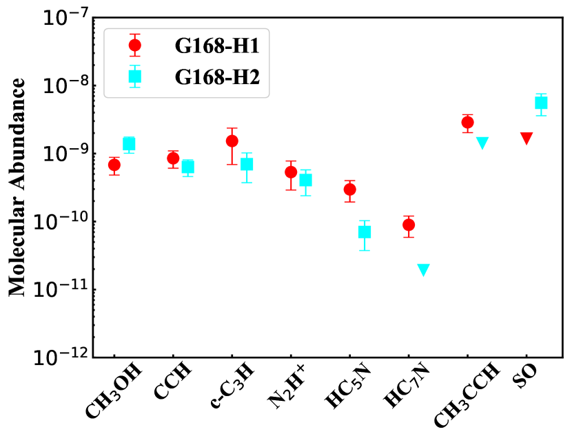
Figure 5: Molecular abundances of observed species (points with error bars) in G168-H1 (red) and G168-H2 (cyan). CH3CCH and HC7N were detected only in the G168-H1 core, and SO was detected only in the G168-H2 core. The down-pointing triangles indicate the upper limits derived from observations.

4 Discussion

4.1 Observed chemical differences between G168-H1 and G168-H2

Figure 5 shows the molecular abundances of all observed species. According to Figure 5, most molecular abundances are lower in G168-H2 than those in G168-H1. It is clear that the carbon-chain molecules (especially for HC5N, HC7N, and CH3CCH) are more abundant in G168-H1 than in G168-H2. Meanwhile, the SO line exhibits an opposite trend compared with other species, showing high abundance in the G168-H2 core and nondetection in the G168-H1 core. G168-H1 and G168-H2 present disparate features in their molecular spectra, gas distributions, and molecular abundances, strongly implying that the two cores likely have different chemical properties.

The carbon-chain molecules CCH and HC5N show stronger line emissions in G168-H1 than those in G168-H2, although the G168-H2 continuum emission is stronger than that of G168-H1. In particular, the HC7N and CH3CCH lines were totally absent in the G168-H2 core. Mapping observations with the PMO also confirm the trend that the carbon-chain molecules are denser in the G168-H1 core than those in the G168-H2 core. From Table 3, one can see that carbon-chain molecules have higher abundances in G168-H1 than those in G168-H2. Carbon-chain molecules may trace the early stages of dense cores, and they have been found to be deficient in the evolved central parts of dense cores (Ohashi et al., 1999; Tafalla et al., 1998; Aikawa et al., 2001). As we mentioned before, G168-H2 seems to be more evolved than G168-H1. The observed differences in the carbon-chain molecular abundances between G168-H1 and G168-H2 are probably due to the fact that they are at different evolutionary stages.

As shown in panel (h) of Figure 2, the SO line emission was detected only in the G168-H2 core. Sulfur-bearing molecules have been found to be depleted in starless and prestellar cores (Tafalla et al., 2006; Agúndez, & Wakelam, 2013; Vastel et al., 2018). Studies of sulfur-bearing molecules suggested that sulfur is initially in the form of S+, which can efficiently produce a S atom by electronic recombination mechanism. Thus, the main reservoirs of sulfur could be a S atom in the gas phase during $10^{3}\sim 10^{5}$ yr in the cold dark clouds. (Bockelée-Morvan et al., 2000; Vidal et al., 2017; Lass & Caselli, 2019). Later, the S atom is consumed by the gas-phase reaction with H3+, CH3, OH, and O2 to efficiently produce SO (Vidal et al., 2017). As G168-H2 is more evolved and denser than G168-H1, there may be sufficient time to produce abundant SO in G168-H2. A possible reason for the nondetection of SO in G168-H1 is that G168-H1 is less evolved; thus, SO may not reach detectable abundance in G168-H1 in a short time.

Figure 3 shows stronger CH3OH line emission in G168-H2 than that in G168-H1. Figure 4 also shows denser gas distribution in G168-H2 than that in G168-H1. CH3OH has been observed in cold dark clouds of TMC-1 CP, L1498, L1517B, and L1544, suggesting that CH3OH is produced on dust grain and then liberated into the gas phase through nonthermal desorption processes in cold dark clouds (Pratap et al., 1997; Takakuwa et al., 2000; Tafalla et al., 2006; Vastel et al., 2014). As shown in panel (c) of Figure 4, the CH3OH gas distribution is well coupled with dust in both G168-H1 and G168-H2. This may indicate that CH3OH originates from grain-surface chemistry (Taquet, Ceccarelli & Kahane, 2012).

Previous observations suggested that N2H+ is mainly concentrated in the center of the core and is more abundant in more evolved dense cores (Tafalla et al., 1998; Crapsi et al., 2005; Sakai et al., 2008). Therefore, N2H+ has been generally used as an evolutionary tracer of dense cores. As stated before, G168-H2 is more evolved than G168-H1. Thus, we would expect that the abundance of N2H+ in G168-H2 is higher than that in G168-H1. However, the G168-H1 and G168-H2 cores have similar N2H+ abundances, which conflicts with the previous studies with higher N2H+ abundances in the evolved cores. Additionally, from panel (b) of Figure 4, one can see that distribution of N2H+ completely covers the dust emission in G168-H1, whereas N2H+ emission is concentrated only in a very small region around the peak of the dust in G168-H2. Lippok et al. (2013) studied seven isolated starless cores by observations and simulations, suggesting that N2H+ is depleted in the center of the cores with hydrogen volume density $\gtrsim$10⁵ cm^-3 and column density $\textgreater$10²² cm^-2. As listed in Table 1, the central H2 volume density and column density of G168-H2 is 1.77($\pm$0.13)$\times$10⁵ cm^-3 and 4.50($\pm$0.01)$\times$10²² cm^-2, respectively. Thus, we speculate that the exceptionally weak emission of N2H+ in G168-H2 may be caused by N2H+ depletion. N2H+ is produced by N2 and destroyed by CO in cold dark clouds by the gas reactions of N2 + H3+ $\rightarrow$ N2H+ + H2 and N2H+ + CO $\rightarrow$ HCO+ + N2, respectively (Aikawa et al., 2001; Bergin et al., 2002). When compared with other prestellar cores and evolved cloud cores, the lower abundance of N2H+ in prestellar core G168-H2 is probably caused by an increase in CO or N2 depletion. Lippok et al. (2013) studied the correlation between C¹⁸O and N2H+ that the N2H+ and C¹⁸O abundances are anticorrelated when the C¹⁸O abundance exceeds 10^-8. As shown in Table 1, the C¹⁸O abundances of G168-H1 and G168-H2 are 1.21($\pm$0.29)$\times$10^-7 and 0.91($\pm$0.29)$\times$10^-7, respectively. Therefore, although destruction by CO is not negligible, we suggest that the N2H+ depletion in the G168-H2 core is dominated by N2 depletion rather than destruction by CO.

4.2 Comparison with other objects

The fractional abundances of carbon-chain molecules in cold dark clouds are approximately $(0.1\sim 4.9)\times 10^{-9}$ for HC5N, $(0.2\sim 7.4)\times 10^{-10}$ for HC7N, and $(0.1\sim 8.1)\times 10^{-9}$ for CH3CCH (Benson & Myers, 1983; Sakai et al., 2008, 2009, 2010; Friesen et al., 2013; Vasyunina et al., 2014; Burkhardt et al., 2018; Mendoza et al., 2018; Seo et al., 2019; Wu et al., 2019). Our observations gave abundances of HC5N, HC7N, and CH3CCH of 2.97($\pm$1.03)$\times$10^-10, 8.95($\pm$3.09)$\times$10^-11, and 2.88($\pm$0.85)$\times$10^-9 in G168-H1, respectively. These values, though at the lower end, are comparable to those of cold dark clouds. However, HC7N and CH3CCH were not detected in G168-H2. Our observations measured an HC5N abundance of only 7.03($\pm$3.28)$\times$10^-11 in G168-H2, which is one order of magnitude lower than those of cold dark clouds. Our results suggest that the starless core G168-H1 may exhibit properties of cold dark clouds, whereas the prestellar core G168-H2 has lower carbon-chain molecular abundances than general cold dark clouds do.

Past studies reported an N2H+ abundance of $(0.7\sim 9)\times 10^{-10}$ in cold dark clouds (Benson, Caselli & Myers, 1998; Bergin et al., 2002; Caselli et al., 2002; Friesen et al., 2010; Taniguchi et al., 2019). The derived N2H+ abundances of G168-H1 and G168-H2 are 5.34($\pm$2.43)$\times$10^-10 and 4.08($\pm$1.68)$\times$10^-10, respectively, which are comparable with previous measurements toward cold dark clouds.

Previous observations reported a CH3OH abundance of $(0.52\sim 47)\times 10^{-9}$ in cold dark clouds (Gómez et al., 2011; Pratap et al., 1997; Requena-Torres et al., 2007; Soma et al., 2015; Tafalla et al., 2006; Vasyunina et al., 2014; Vastel et al., 2014). The estimated abundances of CH3OH are 6.82($\pm$1.99)$\times$10^-10 and 1.38($\pm$0.37)$\times$10^-9 in G168-H1 and G168-H2, respectively, which coincide with those in cold dark clouds. Unlike the abundance differences for the other molecules, the CH3OH abundances are lower in G168-H1 than in G168-H2, indicating that CH3OH shows different chemical properties from carbon-chain and nitrogen-bearing molecules—its abundance increases with core evolution and does not exhibit depletion in PGCC G168.

4.3 Chemical model

To verify the chemical property of the observed molecules in G168-H1 and G168-H2, gas-grain chemical model calculations are highlighted in this section.

We adopt the gas-grain chemical reaction network from Semenov et al. (2010). The gas phase and solid phase are linked through accretion and desorption, which includes both thermal and cosmic-ray-induced desorption processes. In comparison with previous gas-grain models with single-size dust grains (e.g. 0.1 $\mu$m in models of Semenov et al., 2010), the MRN dust size distribution for silicate grains (Mathis, Rumpl & Nordsieck, 1977) is adopted to sample dust grains in the range of 0.005–0.25 $\mu$m in our model. Thus, the size-dependent cosmic-ray desorption proposed by Iqbal & Wakelam (2018) is used as an effective nonthermal mechanism (see more details in Appendix A), which alters the thermal diffusion of species on dust surface and the desorption. Thus, diffusion energy $E_{\rm diff}$ of species controlling the surface reactions becomes more important, which is usually estimated through binding energy $E_{\rm bind}$ with a given diffusion-to-binding energy ratio ($R_{\rm db}$) in the range of 0.3–0.77 (e.g. Semenov et al., 2010). The smaller the $R_{\rm db}$ value is, the faster the thermal diffusion of species is on the dust grain surface. Therefore, $R_{\rm db}$ is also varied to be 0.3, 0.5, and 0.77 to explore the effects of chemistry, particularly for CH3OH, which is mainly formed on dust grains and then can be released by effective desorption. The physical parameters used for G168-H1 and G168-H2 in this study are listed in Table 4, and the determinations of them are presented in Appendix A.

Table 4: Physical Parameters Used for Chemical Models.

Core	$n_{\rm H}$	$T_{\rm gas}$	$T_{\rm dust}$	$A_{\rm V}$	$R_{\rm db}^{a}$
	(cm-3)	(K)	(K)	(mag)
G168-H1	$2\times 10^{4}$	10.0	11.9	10.0	0.3, 0.5, 0.77
G168-H2	$1\times 10^{5}$	10.0	13.2	10.0	0.3, 0.5, 0.77

a: $R_{\rm db}$ is the diffusion-to-binding energy ratio.

For the initial abundances, the low-metal set is used (as listed in Table 5), which has been widely used for dark cloud models (Acharyya & Herbst, 2017; Wakelam, & Herbst, 2008). In addition, the GGCHEM Fortran code was used, which has been successfully benchmarked with various models in Semenov et al. (2010), and has been used to study a number of astrochemical subjects such as the effects of turbulent dust motion on interstellar chemistry (Ge, He & Yan, 2016a) and the chemical differentiation across dust grain sizes (Ge, He & Li, 2016b).

Table 5: Initial Abundances.

Species	$n_{i}/n_{\rm H}$	Species	$n_{i}/n_{\rm H}$
H2	0.5	S+	$8.00\times 10^{-8}$
He	$9.00\times 10^{-2}$	Fe+	$3.00\times 10^{-9}$
C+	$1.20\times 10^{-4}$	Na+	$2.00\times 10^{-9}$
N	$7.60\times 10^{-5}$	Mg+	$7.00\times 10^{-9}$
O	$2.56\times 10^{-4}$	Cl+	$1.00\times 10^{-9}$
Si+	$8.00\times 10^{-9}$	P+	$2.00\times 10^{-10}$

To compare models with observations, we use the chi-squared method to obtain the optimal chemical age for each model by searching for the minimum chi-squared ($\chi^{2}$) using the eight observed molecular abundances listed in Table 3 (see Appendix B). Because of the limited observational data (some species only have upper limits), the optimal chemical age is difficult to be determined precisely by the chi-square method. Therefore, we prefer to use the optimal chemical age range, suggested by the chi-square method, as (2$\sim$3)$\times 10^{5}$ yr and (1$\sim$2)$\times 10^{5}$ yr for G168-H1 and G168-H2, respectively, for further discussion. Because our physical model does not evolve with time, the optimal chemical age is the time scale required for the certain species to reach particular abundances in agreement with the observed abundances, rather than an estimate of the physical age of the real source starts from the diffuse state to the current dense core. Therefore, the chemical age depends on the physical condition of the core and initial chemical abundances and does not reflect the physical age of the core (Maret et al., 2013; Bergin et al., 2006).

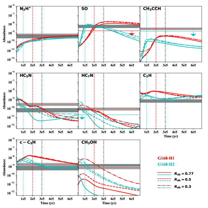
Figure 6: Modeled abundance evolution tracks of molecules (marked by the black label in each panel) in G168-H1 (red) and G168H2 (cyan) with different diffusion-to-binding energy ratios ($R_{\rm db}$) of 0.3 (dashed-dotted line), 0.5 (dashed line), and 0.77 (solid line). The horizontal lines (dotted) with gray regions show the observed values and errors. The horizontal lines (dotted) with arrows show the upper limits derived from observations. The vertical dotted lines indicate the optimal chemical age ranges: (2$\sim$3)$\times 10^{5}$ and (1$\sim$2)$\times 10^{5}$ yr for G168-H1 and G168-H2, respectively. The middle vertical lines (cyan and red) overlap with each other.

Figure 6 shows the modeled abundance evolution tracks of molecules for G168-H1 and G168-H2, together with the observed abundances. From this figure, we see that all of the observed molecular abundances can be well reproduced by our models within one order of magnitude at the abovementioned chemical age ranges (vertical dotted lines).

N2H+ is generally used as a chemical clock because its abundance increases with chemical age monotonously (see Figure 6). However, neither the modeled nor observed abundances of N2H+ in G168-H1 and G168-H2 can be used to constrain their chemical ages owing to the small differences between the two cores. However, the nondetection of SO provides a possible constraint on the chemical age of G168-H1. Compared to SO in G168-H2, which is roughly on the verge of depletion at the median chemical age of $\sim 1.5\times 10^{5}$ yr, SO is less evolved in G168-H1, making it less likely to exhibit a detectable abundance if G168-H1 has a chemical age of $\sim 2\times 10^{5}$ yr. This trend of SO in the G168-H1 model is consistent with that found in other dark cloud models with densities of $\sim 2\times 10^{4}$ cm^-3 (e.g. Agúndez, & Wakelam, 2013; Vidal et al., 2017; Lass & Caselli, 2019). This implies that the nondetection of SO in G168-H1 is due to the less-evolved state of G168-H1. By changing the chemical age of G168-H1 to $\sim$2$\times$10⁵ yr, their observed abundances can also be better reproduced by our models. All these suggest that G168-H1 is less evolved compared with G168-H2 from the viewpoint of chemistry, which is consistent with their physical states indicated by their densities (see Table 4).

According to our models with different diffusion-to-binding ratios ($R_{\rm db}$) of 0.3, 0.5, and 0.77 (see Figure 6), CH3OH is more sensitive to the ratios. This demonstrates that it is mainly formed on dust grains then released by cosmic-ray-induced desorption from small dust grains. The observations exhibit better agreement with models with fast surface reactions ($R_{\rm db}=0.3$ or 0.5), producing comparable abundances of CH3OH within the reasonable chemical age ranges of G168-H1 and G168-H2. Although HC5N and HC7N are also sensitive to the diffusion-to-binding ratios, they are mainly formed in gas-phase at low temperature via dissociative recombination reactions between molecular ions (C2H5N+ and C2H7N+) and electrons (Loison et al., 2014). The dependence of HC5N and HC7N chemistry on diffusion-to-binding energy ratios may mean that HC5N and HC7N formed in the gas phase are absorbed onto dust grains and sublimate into the gas phase by cosmic-ray-induced desorption mechanism. For other carbon-chain molecules, our models also show higher abundances in G168-H1 than those in G168-H2, consistent with the observed trends.

All the modeled features of the observed molecules support the discussion of their chemistry in section 4.1. The chemical difference between the two cores may be due to their different gas densities. As we mentioned in section 1, the G168-H2 core is more evolved and denser than G168-H1. Together with the results of observations and chemical models, we suggest that the chemical difference between the two cores may be due to their different gas densities and different evolutionary stages.

5 Summary

We carried out both observations and model calculations to investigate the chemical properties of the G168-H1 and G168-H2 cores in PGCC G168. The main findings of this work are summarized as follows:

1. Through the single-position observations with the Tianma 65 m telescope, molecular lines of c-C3H, H2CO, and HC5N were detected in both G168-H1 and G168-H2. Whereas HC7N was detected only in G168-H1, and SO was detected only in G168-H2.

2. Mapping observations with the PMO 13.7 m telescope have detected CCH, N2H+, and CH3OH in both G168-H1 and G168-H2 but CH3CCH only in G168-H1. CCH, N2H+, and CH3CCH have stronger emissions in the G168-H1 core than in the G168-H2 core, whereas CH3OH, opposite the distribution of the other three species, presents stronger emission in G168-H2.

3. Carbon-chain species, such as CCH, CH3CCH, HC5N, and HC7N, are less abundant in G168-H2 than in G168-H1. This is consistent with previous studies that carbon-chain molecules are deficient in more evolved prestellar cores.

4. When compared with other prestellar cores, lower N2H+ abundances in the prestellar G168-H2 core can be attributed to N2H+ depletion in the G168-H2 core. We suggest that the N2H+ depletion in G168-H2 is dominated by N2 depletion rather than destruction by CO.

5. By comparison with previous observations of carbon-chain molecules toward various objects, we suggest that the starless core G168-H1 may exhibit the properties of cold dark clouds, but the prestellar core G168-H2 may have an even lower abundance of carbon-chain molecules than general cold dark clouds do.

6. Chemical models have been conducted to explain the observed features in G168. Chemical modeling suggests that the chemical differences between G168-H1 and G168-H2 may be due to their different gas densities and different evolutionary stages.

Appendix A Physical Parameters

Our gas-grain chemical model is a single-point model with fixed physical parameters. The single-point models are set for the core centers of G168-H1 and G168-H2. For the volume densities, we use the typical models of $n_{\rm H}=2\times 10^{4}$ and $n_{\rm H}=1\times 10^{5}$ cm^-3 for G168-H1 and G168-H2 respectively. These values are in accordance with the reported results by Tang et al. (2018), which gives $(1.9\sim 4.6)\times 10^{4}$ and $(0.49\sim 1.8)\times 10^{5}$ cm^-3 for G168-H1 and G168-H2, respectively, from calculations and fitting to column density maps derived from SPIRE continuum data by Marsh et al. (2017). The gas temperature is fixed as 10 K according to the gas kinetic temperatures of 9.66 and 10.25 K for G168-H1 (R.A.=$4^{\rm h}18^{\rm m}33.1^{\rm s}$, Decl.=$28^{\circ}27^{\prime}11^{\prime\prime}$) and G168-H2 (R.A.=$4^{\rm h}18^{\rm m}39.1^{\rm s}$, Decl.=$28^{\circ}23^{\prime}29^{\prime\prime}$) respectively, deduced from NH₃ (1,1) and (2,2) by Seo et al. (2015). We adopted the gas temperatures from NH3(1,1) and (2,2) because they are excellent indicators of temperature (Ho & Townes, 1983; Ungerechts, Walmsley & Winnewisser, 1986; Danby et al., 1988). We tested the effect of temperature on our model and found that the effects of temperature changes between 3 and 10 K were negligible.

Considering the dust component, the dust temperatures are set to 11.9 K and 13.2 K for G168-H1 and G168-H2, respectively (Tang et al., 2018). We have tested models with well-coupled gas and dust temperatures in range of 10–20 K which show that the effects of temperature on chemistry is negligible. Thus, the adopted dust temperatures from the literature is reasonable for our chemical models. Using the relation between extinction and H2 column density proposed by Güver, & Özel (2009), $A_{\rm V}=N(\ce{H2})/2.21\times 10^{21}$ mag, the extinctions are estimated as 6.3 and 11.7 mag for G168-H1 and G168-H2, respectively. Therefore, the visual extinction is fixed as a typical value of 10 mag for both cores. Meanwhile, we used the classical MRN dust size distribution (Mathis, Rumpl & Nordsieck, 1977), which can be expressed as

$$\frac{1}{n_{\rm H}}\frac{dn_{d}}{dr_{d}}=Cr_{d}^{-3.5}dr_{d},\,0.005\leq r_{d}\leq 0.25\,\mu{\rm m},$$ (A1)

where $n_{\rm H}$ is the total number density of H atom, and $r_{d}$ is the dust radius. The grain constant C equals 10^-25.11cm^2.5, as is given by Weingartner & Draine (2001) for silicate grains. Iqbal & Wakelam (2018) had shown that negligible chemical differences resulted from models with dust grains of different bin numbers of 10, 30, and 60. Therefore, we use 10 bins in log-space to represent the dust size distribution to save computation cost. Corresponding to the dust size distribution, size-dependent cosmic-ray-induced desorption is considered in the same way as Iqbal & Wakelam (2018). Namely, the smallest dust grains heat to a peak temperature of $\sim$ 300 K (Herbst & Cuppen, 2006) via collision with a cosmic-ray particle, rather than the 70 K used in the model with single-size dust grains of $r_{d}$=0.1$\micron$ (Hasegawa & Herbst, 1993). The radiation field is fixed as one in units of the FUV interstellar radiation field $\chi_{0}$ from Draine (1978). The cosmic ionization rate is fixed as 3$\times$10^-17 s^-1.

Appendix B Best chemical age

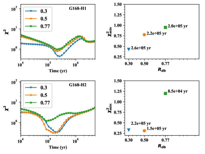
Figure 7: Left panel: $\chi^{2}$ as function of time with varied values of $R_{\rm db}$ as 0.3 (triangle), 0.5 (circle) and 0.77 (square). Right panel: The minimum $\chi^{2}_{\rm min}$ as function of $R_{\rm db}$ showing with the same symbols as that in left panels. The labels show the corresponding best chemical ages. The upper and right panels are for G168-H1 and G168-H2, respectively.

To determine the best chemical ages for G168-H1 and G168-H2, we use the chi-square method, which is expressed as

$$\chi^{2}(t)=\sum_{i=1}^{N}\left[\log(X_{{\rm obs},i})-\log(X_{{\rm mod},i}(t))\right]^{2},$$ (B1)

where $N$ = 8 is the number of observed species including the species only with upper limits determined. $X_{\rm obs}$ and $X_{\rm mod}$ are the observed and modeled abundances of species $i$, respectively. Chi-square ($\chi^{2}$) as a function of chemical age with values of diffusion-to-binding energy ratio ($R_{\rm db}$) of 0.3, 0.5, and 0.77 is shown in the left panels of Figure 7. The right panels show the minimum $\chi^{2}_{\rm min}$ as function of $R_{\rm db}$, with labels indicating the corresponding optimal chemical ages. From this figure, we can see that models with different values of $R_{\rm db}$ have different optimal chemical ages. Because of the limited observed data, the dust properties cannot be constrained. Therefore, we use chemical age ranges to discuss the observed chemical features in this study. The chemical age ranges are (2$\sim$3)$\times 10^{5}$ yr and (1$\sim$2)$\times 10^{5}$ yr for G168-H1 and G168-H2, respectively.

References

- Acharyya & Herbst (2017) Acharyya, K., & Herbst, E. 2017, ApJ, 850, 105
- Agúndez, & Wakelam (2013) Agúndez, M., & Wakelam, V. 2013, Chemical Reviews, 113, 8710
- Aikawa et al. (2001) Aikawa, Y., Ohashi, N., Inutsuka, S., Herbst, E., & Takakuwa, S. 2001, ApJ, 552, 639
- Benson & Myers (1983) Benson, P. J. & Myers, P. C. 1983, ApJ, 270, 589
- Benson, Caselli & Myers (1998) Benson, P. J., Caselli, P., & Myers, P. C. 1998, ApJ, 506, 743
- Bergin et al. (2002) Bergin, E. A., Alves, J., Huard, T. L., & Lada, C. J. 2002, ApJ, 570, 101
- Bergin et al. (2006) Bergin, E. A., Maret, S., van der Tak, F. F. S., et al. 2006, ApJ, 645, 369
- Bockelée-Morvan et al. (2000) Bockelée-Morvan, D., Lis, D. C., Wink, J. E., et al. 2000, A&A, 353, 1101
- Burkhardt et al. (2018) Burkhardt, A. M., Herbst, E., Kalenskii, S., et al. 2018, MNRAS, 474, 5068
- Bussa & VEGAS devolepment team (2012) Bussa, S., & VEGAS Development Team. 2012, in American Astronomical Society Meeting Abstracts, Vol. 219, AAS Meeting, 446.10
- Caselli et al. (2002) Caselli, P., Benson, P. J., Myers, P. C., & Tafalla, M. 2002, ApJ, 572, 238.
- Caselli (2011) Caselli, P. 2011, in IAU Symp. 280, The Molecular Universe, ed. J. Cernicharo & R. Bachiller (Cambridge: Cambridge Univ. Press), 19
- Crapsi et al. (2005) Crapsi, A., Caselli, P., Walmsley, C. M., et al. 2005, ApJ, 619, 379
- Dapp & Basu (2009) Dapp, W. B., & Basu S., 2009, MNRAS, 395, 1092
- Danby et al. (1988) Danby, G., Flower, D. R., Valiron, P., Schilke, P., Walmsley, C. M. 1988, MNRAS, 235, 229
- Draine (1978) Draine, B. T. 1978, ApJS, 36, 595.
- Friesen et al. (2010) Friesen, R. K., Di Francesco, J., Shimajiri, Y., & Takakuwa, S. 2010, ApJ, 708, 1002
- Friesen et al. (2013) Friesen, R. K., Medeiros, L., Schnee, S., et al. 2013, MNRAS, 436, 1513
- Ge, He & Yan (2016a) Ge, J. X., He, J. H., & Yan, H. R. 2016a, MNRAS, 455, 3570
- Ge, He & Li (2016b) Ge, J. X., He, J. H., & Li, A. 2016b, MNRAS, 460, L50
- Gómez et al. (2011) Gómez, L., Wyrowski, F., Pillai, T., Leurini, S., & Menten, K. M. 2011, A&A, 529, 161
- Guilloteau & Lucas (2000) Guilloteau, S., & Lucas, R. 2000, in ASP Conf. Ser. 217, Imaging at Radio through Submillimeter Wavelengths, ed. J. G. Mangum & S. J. E. Radford (San Francisco, CA: ASP), 299
- Güver, & Özel (2009) Güver, T., & Özel, F. 2009, MNRAS, 400, 2050
- Hasegawa & Herbst (1993) Hasegawa, T. I., & Herbst, E. 1993, MNRAS, 261, 83
- Herbst & Cuppen (2006) Herbst, E., & Cuppen, H. M. 2006, Proceedings of the National Academy of Science, 103, 12257
- Hirota & Maezawa (2014) Hirota, T., & Maezawa, H. 2004, ApJ, 617, 399
- Ho & Townes (1983) Ho, P. T. P. & Townes, C. H. 1983, ARA&A, 21, 239H
- Iqbal & Wakelam (2018) Iqbal, W., & Wakelam, V., 2018, A&A, 615, A20
- Lass & Caselli (2019) Laas, Jacob, C. & Caselli, P, 2019, A&A, 624, A108
- Li et al. (2016) Li, J., Shen, Z. -Q., Wang, J., et al. 2016, ApJ, 824, 136
- Li et al. (2017) Li, J., Shen, Z. -Q., Wang, J., et al. 2017, ApJ, 849, 115
- Lippok et al. (2013) Lippok, N., Launhardt, R., Semenov, D., et al. 2013, A&A, 560, A41
- Liu, Wu & Zhang (2012) Liu, T., Wu, Y., & Zhang, H. 2012, ApJS, 202, 4
- Liu et al. (2014) Liu, T., Wu, Y., Mardones, D., et al. 2014, PKAS, 30, 79L
- Liu et al. (2018) Liu, Tie., Kim, Kee-Tae., Juvela, Mika. et al. 2018, ApJS, 234, 28
- Loison et al. (2014) Loison, J. -C., Wakelam, V., Hickson, K. M., Bergeat, A., & Mereau, R. 2014, MNRAS, 437, 930
- Mangum & Shirley (2015) Mangum, J. G. & Shirley, Y. L. 2015, PASP, 127, 266
- Maret et al. (2013) Maret, S., Bergin, E. A., & Tafalla, M. 2013, A&A, 559, A53
- Marsh et al. (2017) Marsh, K. A., Whitworth, A. P., Lomax, O., et al. 2017, MNRAS, 471, 2730
- Mathis, Rumpl & Nordsieck (1977) Mathis, J. S., Rumpl, W., & Nordsieck, K. H., 1977, ApJ, 217, 425
- Mendoza et al. (2018) Mendoza, E., Lefloch, B., Ceccarelli, C. et al. 2018, MNRAS, 475, 5501
- Meng, Wu & Liu (2013) Meng, F., Wu, Y., & Liu, T. 2013, ApJS, 209, 37
- McMullin et al. (2007) McMullin, J. P., Waters, B., Schiebel, D., Young, W., & Golap, K. 2007, Astronomical Data Analysis Software and Systems XVI (ASP Conf. Ser. 376), ed. R. A. Shaw, F. Hill, & D. J. Bell (San Francisco, CA: ASP), 127
- Ohashi et al. (1999) Ohashi, N., Lee, S. W., Wilner, D. J., & Hayashi, M. 1999, ApJL, 518, L41
- Planck Collaboration et al. (2016) Planck Collaboration, Ade, P. A. R., Aghanim, N., et al. 2016, A&A, 594, A28
- Pratap et al. (1997) Pratap, P., Dickens, J. E., Snell, R. L., et al. 1997, ApJ, 486, 862
- Requena-Torres et al. (2007) Requena-Torres, M. A., Marcelino, N., Jiménez-Serra, I., et al. 2007, ApJ, 655, 37
- Sakai et al. (2008) Sakai, N., Sakai, T., Hirota, T., & Yamamoto, S. 2008a, ApJ, 672, 371
- Sakai et al. (2008) Sakai, T., Sakai, N., Kamegai, K., et al. 2008, ApJ, 678, 1049
- Sakai et al. (2009) Sakai, N., Sakai, T., Hirota, T., Burton, M., & Yamamoto, S. 2009, ApJ, 697, 769
- Sakai et al. (2010) Sakai, N., Shiino, T., Hirota, T., Sakai, T., & Yamamoto, S. 2010, ApJL, 718, 49
- Sault, Teuben & Wright (1995) Sault, R. J., Teuben, P. J., & Wright, M. C. H. 1995, in ASP Conf. Ser. 77, Astronomical Data Analysis Software and Systems IV, ed. R. A. Shaw, H. E. Payne, & J. J. E. Hayes (San Francisco, CA: ASP), 433
- Semenov et al. (2010) Semenov, D., Hersant, F., Wakelam, V., et al. 2010, A&A, 522, A42
- Seo et al. (2015) Seo, Y. M., Shirley, Y. L., Goldsmith, P., et al. 2015, ApJ, 805, 185
- Seo et al. (2019) Seo, Y. M., Majumdar, L., Goldsmith, P. F., et al. 2019, ApJ, 871, 134
- Scappini & Codella (1996) Scappini, F., & Codella, C. 1996, MNRAS, 282, 587
- Soma et al. (2015) Soma, T., Sakai, N., Watanabe, Y., & Yamamoto, S. 2015, ApJ, 802, 74
- Suzuki et al. (1992) Suzuki, H., Ymamoto, S., Ohishi, M., et al. 1992, ApJ, 392, 551
- Suzuki, Ohishi & Hirota (2014) Suzuki, T., Ohishi, M., & Hirota, T. 2014, ApJ, 788, 108
- Tafalla et al. (1998) Tafalla,M., Mardones, D., Myers, P. C., et al. 1998, ApJ, 504, 900
- Tafalla et al. (2006) Tafalla, M., Santiago-García, J., Myers, P. C., et al. 2006, A&A, 455, 577
- Tang et al. (2018) Tang, M. Liu, T., Qin, S. -L., et al. 2018, ApJ, 856, 141
- Taniguchi et al. (2018) Taniguchi, K., Saito, M., Sridharan, T. K., & Minamidani, T. 2018, ApJ, 854, 133
- Taniguchi et al. (2019) Taniguchi, K., Saito, M., Sridharan, T. K., & Minamidani, T. 2019, ApJ, 872, 154
- Takakuwa et al. (2000) Takakuwa, S., Mikami, H., Saito, M., et al. 2000, ApJ, 542, 367
- Taquet, Ceccarelli & Kahane (2012) Taquet, V., Ceccarelli, C., & Kahane, C. 2012, A&A, 538, A42
- Ulich & Haas (1976) Ulich & Haas 1976,ApJS, 30, 247
- Ungerechts, Walmsley & Winnewisser (1986) Ungerechts, H., Walmsley, C. M., & Winnewisser, G. 1986, A&A, 157, 207U
- Van der Tak et al. (2007) Van der Tak, F. F. S., Black, J. H., Schöier, F. L., Jansen, D. J., & van Dishoeck, E. F. 2007, A&A, 468, 627
- Vastel et al. (2014) Vastel, C., Ceccarelli, C., Lefloch, B., & Bachiller, R. 2014, ApJL, 795, LL2
- Vastel et al. (2018) Vastel, C., Quénard, D., Le Gal, R., et al. 2018, MNRAS, 478, 5514
- Vasyunina et al. (2014) Vasyunina, T., Vasyunina, A. I., Herbst, E., et al. 2014, APJ, 780, 85
- Vidal et al. (2017) Vidal, Thomas H. G., Loison, Jean-Christophe., Jaziri, A. Y., et al. 2017, MNAS, 469, 435
- Wakelam, & Herbst (2008) Wakelam, V., & Herbst, E. 2008, ApJ, 680, 371
- Wakelam et al. (2010) Wakelam, V., Smith, I. W. M., Herbst, E., et al. 2010, Space Sci. Rev., 156, 13.
- Ward-Thompson et al. (1994) Ward-Thompson, D., Scott, P. F., Hills, R. E., & André, P. 1994, MNRAS, 268, 276
- Ward-Thompson et al. (2016) Ward-Thompson, D., Pattle, K., Kirk, J. M., et al. 2016, MNRAS, 463, 1008
- Weingartner & Draine (2001) Weingartner, J. C., & Draine, B. T., 2001, ApJ, 548, 296
- Wu et al. (2012) Wu, Y., Liu, T., Meng, F., et al. 2012, ApJ, 756, 76
- Wu et al. (2019) Wu, Y,. Lin, L,. Liu, X., et al. 2019, A&A, 627A, 162W
- Zhang et al. (2016) Zhang, T., Wu, Y., Liu, T., et al. 2016, ApJS, 224, 43