Refinement strategies for polygonal meshes applied to adaptive VEM discretization.

Abstract

In the discretization of differential problems on complex geometrical domains, discretization methods based on polygonal and polyhedral elements are powerful tools. Adaptive mesh refinement for such kind of problems is very useful as well and states new issues, here tackled, concerning good quality mesh elements and reliability of the simulations. In this paper we numerically investigate optimality with respect to the number of degrees of freedom of the numerical solutions obtained by the different refinement strategies proposed. A geometrically complex geophysical problem is used as test problem for several general purpose and problem dependent refinement strategies.

1 Introduction

In last years, a growing interest has arised for the development of numerical methods for the solution of partial differential equations using general polygonal meshes. These methods are well suited for handling domains featuring geometrical complexities that can yield situations where the generation of good quality conforming meshes can be particularly expensive or even unfeasible. On the other hand, the use of polygonal and polyhedral elements in conjunction with adaptive mesh refinement states new problems. In this paper we investigate several refinement strategies for polygonal meshes.

As model problem to test the different refinement strategies we consider the simulation of flow in a fractured medium. Flow simulation in underground fractured media is a key aspect in many applications such as aquifers monitoring, nuclear waste disposal, $CO_{2}$ geological storage or control of contaminant dispersion in the subsoil.

In those situations where the rock matrix can be considered perfectly impervious, the Discrete Fracture Network (DFN) model is often used, representing fractures as planar polygons randomly intersected in the 3D space [28, 31, 26, 38]. These kind of domains usually present many geometrical challenges, in particular when a conforming mesh is required, for example in order to apply standard finite element approaches. To circumvent these difficulties, many approaches have been devised, relying on domain decomposition techniques [45, 46], or devising particular meshing strategies [41, 39, 34, 43, 44], or using extensions of the finite element method [12, 36, 33, 37, 6, 35, 42, 29, 4, 32, 25, 40, 3]. In [22, 21, 23], a PDE-constrained optimization approach was devised, enabling for the use of completely non-conforming meshes, where finite element, extended finite element [20] or virtual element spaces [10] can be used. A scalable parallel implementation of such approach is discussed in [24] and a GPU accelerated version in [19]. In [15] and [16], a residual a posteriori error estimate is devised and applied to large scale DFNs. Here we follow the approach based on the Virtual Element Method (VEM) [7, 2, 8, 27] first introduced for DFN flow simulations in [10] and extended in [9, 11, 14].

The huge cost of large scale simulations on the scale of a geological basin raises the issue of efficiency. Moreover, due to the large uncertainty in geometrical configurations and hydrogeological parameters a stochastic approach is advisable yielding to the need of many simulations. Beside efficiency, reliability of these simulations is of crucial importance being connected with risk analysis of human activities. Efficiency and reliability strongly affect the application of uncertainty quantification techniques for the estimation of relevant quantities of interest [17, 18]. For these reasons adaptivity plays a key role both on the side of reliability and efficiency.

Although we focus on the simulation of flow in DFN using VEM, the refinement strategies explored here are suitable for any kind of method relying on polygonal meshes, except for the so-called “Trace Direction” refinement, that is particularly suited for DFN problems taking into account the behaviour of the solution approaching the traces. The approach here followed is based on isotropic “a posteriori” error estimates and aims at generating good quality isotropic polygonal elements. Anisotropic estimates and mesh refinement strategies are currently under investigation in [5].

In Section 2 we introduce the DFN model used to test the refinement strategies and define some useful notations. In Section 3 we introduce its Virtual Element discretization, we define the error estimators and state the “a posteriori” error estimate. In Sections 4 and 5 we describe the initial mesh generation, the adaptive algorithm, and the polygonal refinement strategies. In Section 6 we validate their application to some test cases with known solution, and, in Section 7, we analyse some results on a more realistic DFN.

2 Discrete Fracture Networks

Let us consider a set of open convex planar polygonal fractures $F_{i}\subset\mathbb{R}^{3}$ with $i=1,...,N$, with boundary $\partial F$. A DFN is $\Omega=\bigcup_{i}F_{i}$, with boundary $\partial\Omega$. Even though the fractures are planar, their orientations in space are arbitrary, such that $\Omega$ is a 3D set. The set $\Gamma_{D}\subset\partial\Omega$ is where Dirichlet boundary conditions are imposed, and we assume $\Gamma_{D}\neq\emptyset$, whereas $\Gamma_{N}=\partial\Omega\setminus\Gamma_{D}$, is the portion of the boundary with Neumann boundary conditions. Dirichlet and Neumann boundary conditions are prescribed by the functions $h^{D}\in\mathrm{H}^{\frac{1}{2}}\!\left(\Gamma_{D}\right)$ and $g^{N}\in\mathrm{H}^{-\frac{1}{2}}\!\left(\Gamma_{N}\right)$ on the Dirichlet and Neumann part of the boundary, respectively. We further set $\Gamma_{iD}=\Gamma_{D}\cap\partial F_{i}$, $\Gamma_{iN}=\Gamma_{N}\cap\partial F_{i}$, and $h_{i}^{D}={h^{D}}_{|\Gamma_{iD}}$ and $g_{i}^{N}={g^{N}}_{|\Gamma_{iN}}$. The set $\mathcal{S}$ collects all the traces, i.e. the intersections between fractures, and each trace $S\in\mathcal{S}$ is given by the intersection of exactly two fractures, $S=\bar{F}_{i}\cap\bar{F}_{j}$, such that there is a one to one relationship between a trace $S$ and a couple of fracture indices $\{i,j\}=\mathcal{I}(S)$. We will also denote by $\mathcal{S}_{i}$ the set of traces belonging to fracture $F_{i}$.

Subsurface flow is governed by the gradient of the hydraulic head $H=\mathcal{P}+\zeta$, where $\mathcal{P}=p/(\varrho g)$ is the pressure head, $p$ is the fluid pressure, $g$ is the gravitational acceleration constant, $\varrho$ is the fluid density and $\zeta$ is the elevation.

We define the following functional spaces:

$$V_{i} =\mathrm{H}^{1}_{\rm 0}\left(F_{i}\right)=\left\{v\in\mathrm{H}^{1}\!\left(F_{i}\right):v_{|_{\Gamma_{iD}}}=0\right\},$$

$$V_{i}^{D} =\mathrm{H}^{1}_{\rm D}\left(F_{i}\right)=\left\{v\in\mathrm{H}^{1}\!\left(F_{i}\right):v_{|_{\Gamma_{iD}}}=h_{i}^{D}\right\},$$

and

$$V=\left\{v\colon{v}_{|F_{i}}\in V_{i},\ \forall i\!=\!1,\ldots,N,\gamma_{S}(v_{|F_{i}})\!=\!\gamma_{S}(v_{|F_{j}}),\;\forall S\!\in\!\mathcal{S}_{i},\ \{i,j\}\!=\!\mathcal{I}(S)\right\}\,,$$

$$V^{D}=\left\{v\colon{v}_{|F_{i}}\in V_{i}^{D}\!\!,\ \forall i\!=\!1,\ldots,N,\gamma_{S}(v_{|F_{i}})\!=\!\gamma_{S}(v_{|F_{j}}),\;\forall S\!\in\!\mathcal{S}_{i},\ \{i,j\}\!=\!\mathcal{I}(S)\right\}\,,$$

where $\gamma_{S}$ is the trace operator onto $S$. In order to formulate the DFN flow problem, let us define ${a}_{i}\colon V_{i}^{D}\times V_{i}\to\mathbb{R}$ be defined as

$${a}_{i}\left(w,v\right)=\left(\mathcal{K}_{i}\nabla\left({w}_{|F_{i}}\right),\nabla\left({v}_{|F_{i}}\right)\right)_{F_{i}}\quad\forall w\in V^{D},\ v\in V\,,$$

where $\mathcal{K}_{i}$ is the fracture transmissivity tensor, that we assume to be constant on each fracture. Let us denote by $H\in V^{D}$ the hydraulic head on the DFN and by $H_{i}\in V_{i}^{D}$ its restriction to the fracture $F_{i}$ and by $v\in V$ the test functions. Assuming the hydraulic head modelled by the Darcy law, the whole problem on the DFN is: find $H\in V^{D}$ such that $\forall v\in V$

$$\sum_{i=1}^{N}{a}_{i}\left(H_{i},v\right)=\sum_{i=1}^{N}\left(f_{i},v\right)_{F_{i}}+g_{i}^{N}{}{\mathrm{H}^{-\frac{1}{2}}\!\left(\Gamma_{N_{i}}\right),\mathrm{H}^{\frac{1}{2}}\!\left(\Gamma_{N_{i}}\right)}.$$ (1)

3 Virtual Element discretization

In this section we describe the Virtual Element discretization of equation (1) assuming a globally conforming polygonal mesh is given on the DFN. A globally conforming mesh ia a polygonal mesh on each fractures such that polygon edges match exactly at traces. In Section 4 we devise a way to obtain a mesh of this type and Section 5 describes some refinement strategies that preserve the global conformity of the mesh.

Let $\mathcal{T}_{\delta}$ be a globally conforming polygonal mesh of $\Omega$ fulfilling the regularity requirements needed by the Virtual Element method [8], $E\in\mathcal{T}_{\delta}$ be any polygon of this tessellation. Let $\mathbb{P}_{k}\!\left(E\right)$ be the space of polynomials of degree $\leq k$ defined on $E$. To define the discrete functional space on $E$, we introduce the $\mathrm{H}^{1}$-orthogonal projector $\Pi^{\nabla}_{k,E}\colon\mathrm{H}^{1}\!\left(E\right)\to\mathbb{P}_{k}\!\left(E\right)$ such that

$$\left(\nabla\left(v-\Pi^{\nabla}_{k,E}v\right),\nabla p\right)_{E}=0\,,\forall p\in\mathbb{P}_{k}\!\left(E\right)$$

and

$$\begin{cases}\left(\Pi^{\nabla}_{k,E}v,1\right)_{\partial E}=\left(v,1\right)_{\partial E}&\text{if $k=1$}\,,\\ \left(\Pi^{\nabla}_{k,E}v,1\right)_{E}=\left(v,1\right)_{E}&\text{if $k\geq 1$}\,.\end{cases}$$

The Virtual Element space of order $k\in\mathbb{N}$ on $E$ is defined as

$$V_{\delta}^{E}=\left\{v\in\mathrm{H}^{1}\!\left(E\right)\colon\Delta v\in\mathbb{P}_{k}\!\left(E\right),\,v\in\mathbb{P}_{k}\!\left(e\right)\,\forall e\subset\partial E,\gamma^{\partial E}\!\left(v\right)\in C^{0}\!\left(\partial E\right)\,,\right.\\ \quad\left.\left(v,p\right)_{E}=\left(\Pi^{\nabla}_{k,E}v,p\right)_{E}\,\forall p\in\mathbb{P}_{k}\!\left(E\right)/\mathbb{P}_{k-2}\!\left(E\right)\right\}\,,$$

where $\mathbb{P}_{k}\!\left(E\right)/\mathbb{P}_{k-2}\!\left(E\right)$ denotes the subspace of $\mathbb{P}_{k}\!\left(E\right)$ containing polynomials that are $\mathrm{L}^{2}\!\left(E\right)$-orthogonal to $\mathbb{P}_{k-2}\!\left(E\right)$. Furthermore, let us denote by $\mathcal{T}_{\delta,i}$ the restriction of $\mathcal{T}_{\delta}$ to fracture $F_{i}$. The Virtual Element space on $\mathcal{T}_{\delta,i}$ is

$$V_{\delta,i}=\left\{v\in C^{0}\!\left(F_{i}\right)\colon v\in V_{\delta}^{E}\;\forall E\in\mathcal{T}_{\delta,i}\right\}\,.$$

Since $\mathcal{T}_{\delta}$ is globally conforming, we can define the global discrete spaces as

$$V_{\delta} =\left\{v\in V\colon v_{|F_{i}}\in V_{\delta,i}\right\}\,, V_{\delta}^{D} =\left\{v\in V^{D}\colon v_{|F_{i}}\in V_{\delta,i}\right\}\,.$$

A function in the above space is uniquely identified by the following set of degrees of freedom:

1. the values at the vertices of the polygons;

2. if $k\geq 2$, for each edge $e$ of the mesh, the value of $v$ at $k-1$ internal points of $e$;

3. if $k\geq 2$, for each $E\in\mathcal{T}_{\delta}$, the scaled moments $\frac{1}{\left\lvert{E}\right\rvert}\left(v,m_{\boldsymbol{\alpha}}\right)_{E}$ for all the scaled monomials $m_{\boldsymbol{\alpha}}$, with $\boldsymbol{\alpha}=\left(\alpha_{1},\alpha_{2}\right)$, $\left\lvert{\boldsymbol{\alpha}}\right\rvert=\alpha_{1}+\alpha_{2}\leq k-2$, such that

   $$\forall(x,y)\in E,\quad m_{\boldsymbol{\alpha}}(x,y):=\frac{(x-x_{E})^{\alpha_{1}}(y-y_{E})^{\alpha_{2}}}{h_{E}^{\alpha_{1}+\alpha_{2}}}\,,$$

   being $(x_{E},y_{E})$ the centroid of the cell and $h_{E}$ its diameter.

For any element $E\in\mathcal{T}_{\delta}$, given a function $v_{\delta}\in V_{\delta}^{E}$, it can be seen [7, 47] that the values of its degrees of freedom are uniquely defined by its $\mathrm{L}^{2}\!\left(E\right)$-orthogonal projection on $\mathbb{P}_{k-1}\!\left(E\right)$, denoted by $\Pi^{0}_{k-1,E}v_{\delta}$, and the orthogonal projection of its gradient on $\mathbb{P}_{k-1}\!\left(E\right)\times\mathbb{P}_{k-1}\!\left(E\right)$, denoted by $\Pi^{0}_{k-1,E}\nabla v_{\delta}$. A basis of the local VEM space is defined implicitly as the set of functions that are Lagrangian with respect to the degrees of freedom.

To discretize (1) by the Virtual Element method we suppose to know, for each $E\in\mathcal{T}_{\delta,i}$, $i=1,\ldots,N$, a bilinear form $S\colon V_{\delta}^{E}\times V_{\delta}^{E}\to\mathbb{R}$ such that, $\forall v_{\delta}\in V_{\delta}^{E}\cap\ker\Pi^{\nabla}_{k,E}$,

$$\exists c_{\ast}\,,c^{\ast}>0\colon c_{\ast}\left(\mathcal{K}_{i}\nabla v_{\delta},\nabla v_{\delta}\right)_{E}\leq S^{E}\left(v_{\delta},v_{\delta}\right)\leq c^{\ast}\left(\mathcal{K}_{i}\nabla v_{\delta},\nabla v_{\delta}\right)_{E}\,.$$

With the above assumption, we define, for each $E\in\mathcal{T}_{\delta,i}$, $i=1,\ldots,N$, the bilinear form ${a}^{E}_{\delta}\colon V_{\delta}^{E}\times V_{\delta}^{E}\to\mathbb{R}$ such that, $\forall u_{\delta},v_{\delta}\in V_{\delta}$,

$${a}^{E}_{\delta}\left(u_{\delta},v_{\delta}\right)=\left(\mathcal{K}_{i}\Pi_{k-1}^{0}\nabla u_{\delta},\Pi^{0}_{k-1}\nabla v_{\delta}\right)_{E}+\mathcal{K}_{i}S^{E}\left(\left(I-\Pi^{\nabla}_{k}\right)u_{\delta},\left(I-\Pi^{\nabla}_{k}\right)v_{\delta}\right)\,,$$

and the global bilinear form ${a}_{\delta}\colon V_{\delta}^{D}\times V_{\delta}\to\mathbb{R}$ such that

$${a}_{\delta}\left(u_{\delta},v_{\delta}\right)=\sum_{i=1}^{N}\sum_{E\in\mathcal{T}_{\delta,i}}{a}^{E}_{\delta}\left({u_{\delta}}_{|F_{i}},{v_{\delta}}_{|F_{i}}\right).$$

Finally, the Virtual Element discretization of (1) is: find $H_{\delta}\in V_{\delta}^{D}$ such that, $\forall v_{\delta}\in V_{\delta}$

$${a}_{\delta}\left(H_{\delta},v_{\delta}\right)=\sum_{i=1}^{N}\left(\sum_{E\in\mathcal{T}_{\delta,i}}\left(f_{i},\Pi^{0}_{k-1,E}\!\left({v}_{|F_{i}}\right)\right)_{E}\right)\\ +g_{i}^{N}{}{\mathrm{H}^{-\frac{1}{2}}\!\left(\Gamma_{N_{i}}\right),\mathrm{H}^{\frac{1}{2}}\!\left(\Gamma_{N_{i}}\right)}\,.$$ (2)

We remark that the continuity conditions are automatically satisfied by the definition of the functional space and the degrees of freedom, viable because $\mathcal{T}_{\delta}$ is a globally conforming discretization.

In [14], a residual a posteriori estimate was derived for the Laplace problem proving the equivalence between the estimator and the error with respect to a suitable polynomial projection of the VEM solution. The extension of this estimate to the case of a globally conforming discretization of the Laplace problem on a DFN is quite straightforward. Let us define the following error measure:

$$\left\lvert\left\lvert\left\lvert v\right\rvert\right\rvert\right\rvert=\sup_{w\in V}\frac{\sum_{i=1}^{N}{a}_{i}\left(v_{i},w\right)}{\left(\sum_{i=1}^{N}\left\lVert{\sqrt{\mathcal{K}}\nabla w}\right\rVert_{F_{i}}^{2}\right)^{\frac{1}{2}}}\,,$$

then, we denote $H_{\delta}^{\pi}=\Pi^{\nabla}_{k}\!\left(H_{\delta}\right)$ and define

$$est_{\delta}^{2}=\sum_{i=1}^{N}\left(\sum_{E\in\mathcal{T}_{\delta,i}}\frac{h^{2}_{E}}{\mathcal{K}_{i}}\left\lVert{\Pi^{0}_{k-1}f+\mathcal{K}_{i}\Delta H_{\delta i}^{\pi}}\right\rVert_{E}^{2}+\sum_{e\in\mathcal{E}_{\delta,i}^{\textrm{int}}}\frac{h_{e}}{\mathcal{K}_{i}}\left\lVert{\left\llbracket{\mathcal{K}_{i}\frac{\partial H_{\delta i}^{\pi}}{\partial\mathbf{n}}}\right\rrbracket_{e}}\right\rVert_{e}^{2}+\right.\\ \left.+\sum_{e\in\mathcal{E}_{\delta,i}^{N}}\frac{h_{e}}{\mathcal{K}_{i}}\left\lVert{\left\llbracket{\mathcal{K}_{i}\frac{\partial H_{\delta i}^{\pi}}{\partial\mathbf{n}}}\right\rrbracket_{e}-g_{i}^{N}}\right\rVert_{e}^{2}+\sum_{E\in\mathcal{T}_{\delta}}\frac{h^{2}_{E}}{\mathcal{K}_{i}}\left\lVert{f-\Pi^{0}_{k-1}f}\right\rVert_{E}^{2}\right)\\ +\sum_{\begin{subarray}{c}S\in\mathcal{S}\colon\\ \mathcal{I}(S)=\{i,j\}\end{subarray}}\left(\sum_{e\in\mathcal{E}_{\delta,S}}\frac{h_{e}}{\min\{\mathcal{K}_{i},\mathcal{K}_{j}\}}\left\lVert{\left\llbracket{\mathcal{K}_{i}\frac{\partial H_{\delta i}^{\pi}}{\partial\mathbf{n}}}\right\rrbracket_{e}+\left\llbracket{\mathcal{K}_{j}\frac{\partial H_{\delta j}^{\pi}}{\partial\mathbf{n}}}\right\rrbracket_{e}}\right\rVert_{e}^{2}\right)\,,$$

where $\forall i=1,\ldots N$, $\mathcal{E}_{\delta,i}^{\textrm{int}}$ is the set of edges of $\mathcal{T}_{\delta,i}$ such that, $\forall e\in\mathcal{E}_{\delta,i}^{\textrm{int}}$, $e\cap S=\emptyset$ $\forall S\in\mathcal{S}_{i}$ and $e\cap\Gamma_{N_{i}}=\emptyset$, $\mathcal{E}_{\delta,i}^{N}$ is the set of edges $e$ of $\mathcal{T}_{\delta,i}$ such that $e\cap\Gamma^{N}_{i}\neq\emptyset$ and $\forall S\in\mathcal{S}$, $\mathcal{E}_{\delta,S}$ is the set of edges $e$ of $\mathcal{T}_{\delta}$ such that $e\cap S\neq\emptyset$. Then, there exist two constants $c,C>0$ independent of $\delta$ such that

$$c\cdot est_{\delta}\leq\left\lvert\left\lvert\left\lvert H-H_{\delta}^{\pi}\right\rvert\right\rvert\right\rvert\leq C\cdot est_{\delta}\,.$$ (3)

In view of an adaptive approach, we define, for each cell $E$, a local estimator $est_{\delta,E}$, such that the estimators defined on the edges are split among neighbouring cells according to their areas.

4 DFN Minimal mesh construction

In this section we introduce the strategy used for the construction of the initial coarse polygonal mesh on the DFNs. This mesh is obtained by the construction of convex polygons representing sub-fractures, i.e. portion of fractures not crossed by traces that can have traces or portion of traces or extension of traces only on the boundary. Given a fracture and the set of its traces there exist many partitions of the fracture in sub-fractures with a different number of sub-fractures and different quality of the element produced. The construction of the minimal mesh is a complex trade off between the number of the elements and the quality of the elements produced. In our approach we aim at limiting the number of elements. Improvement of the mesh quality is transferred to a following suitable refining strategy.

The approach we follow is an iterative splitting of the leaves of a tree structure. We start from the original fracture that is the root cell of the structure, then we select a trace and we split the given cell along the trace or an extension of the trace producing two children cells. Then we proceed iteratively choosing a new trace and cutting the leaves of the tree with the selected trace, exclusively in the case the trace is intersecting the internal part of the cell. At each iteration each cell can be split in two children cells or can be modified in a unique child cell that is the same polygon with one of the edges split in two aligned sub-edges in order to guarantee conformity of the global mesh. The algorithm is sketched in Algorithm 1.

In order to control the number of cells produced by the algorithm we cut the current cells with a suitable order of traces. We start considering the traces that cross the fracture intersecting two boundary edges of the fracture. Then we continue considering the remaining traces from the longest to the shortest. Considering the traces in this order usually yields to a smaller number of cells.

Algorithm 1 Minimal mesh

Given a fracture and the set of traces create a tree structure with the fracture as root cell

1:  for All the traces do

2:     for All the leaves cells of the tree do

3:        Compute the intersection of the trace with the cell

4:        if There is an intersection with the internal part of the cell then

5:           Split the cell in two children cells

6:        end if

7:        Update the neighbouring cell with the new edges

8:     end for

9:  end for

5 Refinement and Marking algorithms

In this section we briefly introduce the algorithms used for marking the cells with largest estimators to be refined in order to reduce the discretization error and the different algorithms tested for the refinement of polygonals cells. This refinement step is part of the usual refinement process SOLVE-ESTIMATE-MARK-REFINE [30].

5.1 Marking Strategy

The marking strategy (see Algorithm 2) of the cells to be refined is simply based on the selection of all the cells with the largest error estimators. We mark the cells starting from those with largest estimators $est_{\delta,E}^{2}$ up to when the cumulative error estimator $est_{\delta,\mathcal{T}_{\delta,mark}}^{2}$ of the marked cells is a given ratio $C$ of the total error estimator $est_{\delta,\mathcal{T}_{\delta}}^{2}=\sum_{E\in\mathcal{T}_{\delta}}est_{\delta,E}^{2}$. In this algorithm we accept the sorting cost for the estimators vector [30] in order to maximally contain the refinement iterations that, in practical applications to large scale DFN simulations, can be quite expensive in the last refinement steps.

Algorithm 2 Cells marking algorithm

Given a convex polygon

1:  Compute the cell error estimators $est_{\delta,E}^{2}$ and save them in a vector $Vest_{\delta}^{2}$.

2:  Compute the total error estimator $est_{\delta,\mathcal{T}_{\delta}}^{2}$

3:  Sort the cell estimators vector $Vest_{\delta}^{2}$

4:  Choose a constant $0<C<1$

5:  $i=0$

6:  $est_{\delta,\mathcal{T}_{\delta,mark}}^{2}=est_{\delta,\mathcal{T}_{\delta,mark}}^{2}+Vest_{\delta}^{2}(i)$

7:  repeat

8:     $i++$

9:     $est_{\delta,\mathcal{T}_{\delta,mark}}^{2}=est_{\delta,\mathcal{T}_{\delta,mark}}^{2}+Vest_{\delta}^{2}(i)$

10:  until $est_{\delta,\mathcal{T}_{\delta,mark}}^{2}\leq C*est_{\delta,\mathcal{T}_{\delta}}^{2}$

11:  Mark the cells corresponding to the first $i$ positions of $Vest_{\delta}^{2}$

5.2 Refinement algorithms

In this section we introduce four different refinement algorithms used for cutting marked convex cells in two convex sub-cells. All the algorithms are based on a similar approach and differ for the choice of the cutting direction. The common approach is described in the Algorithm 3 and the four different approaches differ for the Step 3 of Algorithm 3.

Algorithm 3 Refinement algorithm for convex polygons

Given a convex polygon

1:  Check aspect ratio (AR)

2:  Compute the centroid $\mathbf{X}_{c}$

3:  Choose the cutting direction

4:  Build a straight line passing from the centroid with the chosen direction

5:  Choose the collapsing tolerance CollapseToll

6:  for Each edges of the cell do

7:     if There is an intersection then

8:        if The intersection point is near to the begin/end point of the edge according to the chosen tolerance CollapseToll then

9:           Change the cutting direction and set the intersection point as the begin/end point of the edge

10:        else

11:           The intersection point will be a new point in the mesh

12:        end if

13:     end if

14:  end for

15:  Create the two children cells

16:  Update the neighbourhood

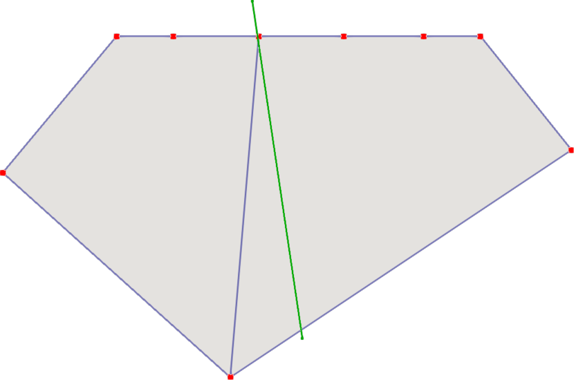
(a) Maximum Momentum

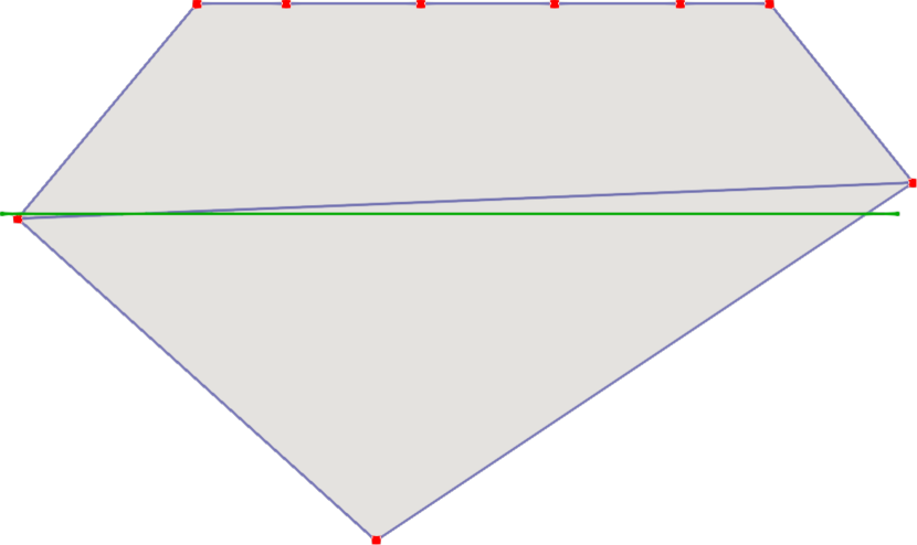
(b) Trace Direction

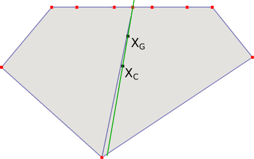
(c) Maximum Number of Points

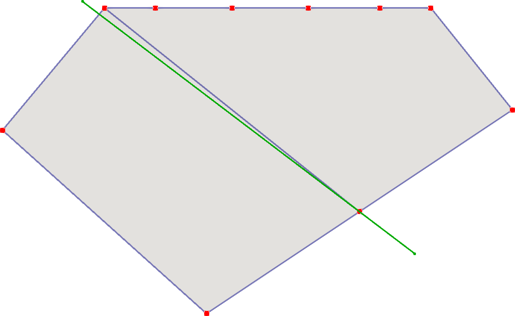
(d) Maximum Edge

Figure 1: Different strategies for the selection of the cutting direction.

In the following we compare four different refinement options for choosing the cutting direction denoted Maximun Momentum (MaxMom), Trace Direction (TrDir), Maximum Number of Points (MaxPnt) and Maximum Edge (MaxEdg). At the Step 8 of the Algorithm 3 we accept to slightly modify the chosen cutting direction in order to avoid the proliferation of edges and vertices of the new cells and consequently of VEM degrees of freedom that do not efficiently increase the quality of the solution and to avoid the generation of very small edges that could sometimes induce stability problems [27, 13].

We collapse the points given by the intersection of the cutting direction with an edge to existing vertices of the cell when the distance of the intersection from the closest vertex are smaller than the tolerance CollapseToll multiplied by the length of the edge intersected.

For some of the proposed cutting directions we switch from the selected refinement criterion to the Maximum Momentum criterion in order to avoid the generation of cells with a huge aspect ratio (AR) defined as the ratio between the longest distance between the centroid and the vertices and the smallest distance between the centroid and the edges. In order to avoid the generation of elements with a huge aspect ratio, we define a fixed value denoted by MaxAR and if the aspect ratio of the cell to cut is larger than MaxAR, the cutting criterion is always MaxMom.

5.2.1 Maximum Momentum (MaxMom)

This cutting strategy of marked cells is based on the choice of cutting direction that is orthogonal to the direction of eigenvector associated to the smallest eigenvalue of the inertia tensor of the cell (Figure 1(a)).

5.2.2 Trace Direction (TrDir)

This cutting strategy is based on the choice as cutting direction of the direction parallel to a trace (if any), see Figure 1(c), where we have assumed that the edge with several aligned points belongs to the trace. The rationale of this approach is related to the known property of the solution to the considered problem that displays strong gradient components in the direction orthogonal to the traces. If a cell intersects more than one trace we switch to MaxMom criterion.

5.2.3 Maximum Number of Points (MaxPnt)

This cutting strategy is based on the choice as cutting direction of the direction of the vector connecting the centroid of the cell $X_{C}$ to the center of mass of the vertices $X_{G}$, see Figure 1(c). This vector points towards the region of the marked cell with the highest density of vertices and should split the cell balancing the vertices of the two new subcells. In this strategy it is mandatory to define the option MaxNP, to set how many points the cells can have. This strategy switches to the MaxMom strategy in two cases: the first when the number of points of the cell to cut is less than MaxNP, the second when the centroid and the center of mass have a distance under a fixed tolerance. We remark that this refinement strategy can be considered as a simple improvement of the MaxMom strategy being the refinement strategy different only for the cells with a large number of cells and considering that when the number of vertices of the cell is larger than MaxNP this refinement strategy aims at dropping the number of vertices of the two produced cells under MaxNP.

5.2.4 Maximum Edge (MaxEdg)

This cutting strategy is based on the choice as cutting direction of the direction that cuts the longest edge of the cell in half, see Figure 1(d), where the longest edge is the right-bottom edge. If a cell displays aligned edges, these are considered as one unique edge.

6 Numerical Results: optimality and effectivity index

In order to validate our refinement algorithm we test it on two simple DFNs for which an exact solution is known. We consider two DFNs with two and three fractures, labelled as Problem 1 and Problem 2, respectively.

This first set of tests aims at validating the equivalence relation stated in (3) between the error and the error estimator. We have tested this equivalence relation on the meshes produced during the adaptive process although this property holds true on any sufficiently refined mesh. We apply our adaptive algorithm and compare at each refinement iteration the error and the error estimator computing the effectivity index

$$\varepsilon=\frac{err}{est_{\delta}}$$

in order to verify that it is independent of the mesh size obtained by adaptive refinements. See [14] for the same analysis performed on uniformly refined meshes.

As stopping criterion for the adaptive process, we require the following condition on the estimated relative error:

$$\frac{est_{\delta}}{\left(\sum_{i=1}^{N}\left\lVert{\sqrt{\mathcal{K}_{i}}\nabla\Pi^{\nabla}_{k}H_{\delta i}}\right\rVert_{F_{i}}^{2}\right)^{\frac{1}{2}}}\leq 0.05\,.$$ (4)

All the simulations here presented are performed with the following methods and parameters: VEM orders from $1$ to $4$, Preconditioned Conjugate Gradient as linear solver with relative stopping residual $1.0e-15$, the preconditioner being an incomplete Cholesky factorization implemented as described in [1], CollapseToll = 0.2, MaxAR = 10, MaxNP = 12 and C = 0.50.

6.1 Problem $1$

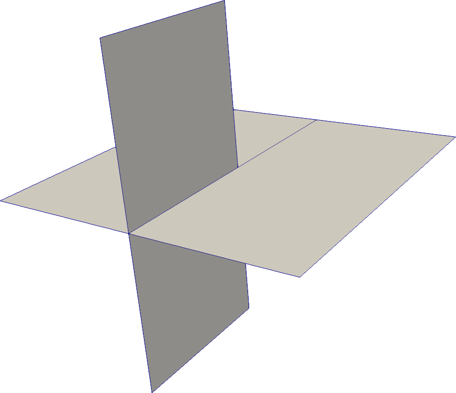
(a) Initial mesh

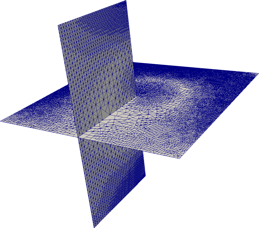
(b) Step 30 MaxMom

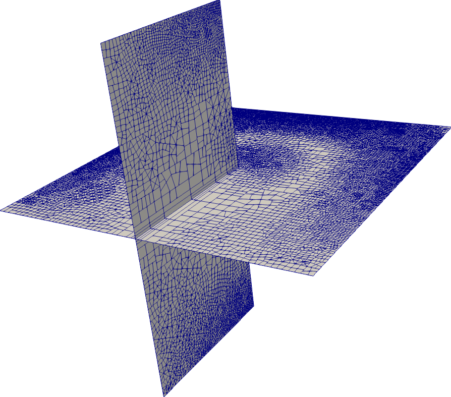
(c) Step 30 TrDir

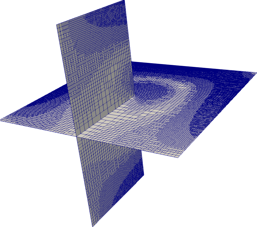
(d) Step 30 MaxEdg

Figure 2: Problem 1: DFN with meshes at refining step 30.

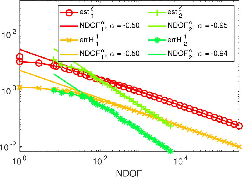
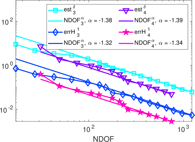
Figure 3: Problem 1: Rates of convergence ($\alpha$) for error and estimator with MaxMom refinement.

TypeRef	Order 1	Order 2	Order 3	Order 4
MaxMom	$\alpha=-0.50$	$\alpha=-0.95$	$\alpha=-1.38$	$\alpha=-1.39$
	$\alpha_{err}=-0.50$	$\alpha_{err}=-0.94$	$\alpha_{err}=-1.32$	$\alpha_{err}=-1.34$
TrDir	$\alpha=-0.49$	$\alpha=-0.93$	$\alpha=-1.67$	$\alpha=-1.56$
	$\alpha_{err}=-0.50$	$\alpha_{err}=-0.92$	$\alpha_{err}=-1.63$	$\alpha_{err}=-1.30$
MaxEdg	$\alpha=-0.50$	$\alpha=-0.93$	$\alpha=-1.37$	$\alpha=-1.55$
	$\alpha_{err}=-0.50$	$\alpha_{err}=-0.93$	$\alpha_{err}=-1.41$	$\alpha_{err}=-1.38$

Table 1: Problem 1: Rates of convergence for the estimator ($\alpha$) and the error ($\alpha_{err}$) with refinement criteria MaxMom, TrDir and MaxEdg.

Step	$\#$ Cells	NDOF	$\varepsilon$	PCG-It
1	4	1	0.0064	1
5	16	8	0.0221	5
10	58	44	0.0318	12
15	232	208	0.0326	23
20	958	910	0.0345	43
25	3997	3901	0.0343	88
30	16696	16214	0.0337	181
35	69827	67074	0.0334	370
39	219297	207112	0.0333	662
40	291581	274982	0.0332	777

Table 2: Problem 1: MaxMom refinement Order 1.

Step	$\#$ Cells	NDOF	$\varepsilon$	PCG-It
1	4	1	0.0064	1
5	14	5	0.0130	1
10	46	34	0.0441	12
15	167	147	0.0364	21
20	672	712	0.0356	46
25	2760	3232	0.0377	94
30	11528	13848	0.0357	188
35	48362	57738	0.0353	378
39	152185	178922	0.0349	695
40	202798	237727	0.0347	846

Table 3: Problem 1: TrDir refinement Order 1.

Step	$\#$ Cells	NDOF	$\varepsilon$	PCG-It
1	4	1	0.0064	1
5	16	7	0.0271	3
10	58	43	0.0347	12
15	239	223	0.0381	21
20	974	1007	0.0382	47
25	4101	4420	0.0382	100
30	17254	18980	0.0380	205
35	72401	80561	0.0386	414
37	128831	139214	0.0385	545

Table 4: Problem 1: MaxEdg refinement Order 1.

The geometry and the parameters of this test problem are described in detail in [21, Section 5.1]. The DFN is composed by two fractures that are planar rectangles defined as

$$F_{1}=(-1,1)\times(-1,1)\times\{0\}\,;\quad F_{2}=(-1,0)\times\{0\}\times(-1,1)\,.$$

Thus, the only trace of the DFN is $\Gamma_{1}=(-1,0)\times\{0\}\times\{0\}$. The differential model is set up by choosing the following exact solutions:

$$h_{1}(x,y,z) =\left(x^{2}-1\right)\left(y^{2}-1\right)\left(x^{2}+y^{2}\right)\cos\left(\frac{1}{2}\mathrm{arctan2}(x,y)\right)\,,$$

$$h_{2}(x,y,z) =-\left(z^{2}-1\right)\left(x^{2}-1\right)\left(x^{2}+z^{2}\right)\cos\left(\frac{1}{2}\mathrm{arctan2}(z,x)\right)\,,$$

where $\mathrm{arctan2}(x,y)$ is the four-quadrant inverse tangent, that is the $\mathrm{arctan}$ of $y/x$ in $[-\pi,\pi]$. The transmissivity of both fractures is set to $1$.

In Figure 2 we report some of the meshes generated during the refinement process. We remark that in this test problem the presence of a known forcing function on the fractures induces a refinement in the whole domain, this will not be the same for the flow simulations in which the rock matrix surrounding the DFNs is considered impervious (Section 7).

In Figure 3 we report the convergence behaviour of the error (errH¹) and of the error estimator (est_δ) and the final rates of convergence $\alpha$ with respect to the total number of degrees of freedom (NDOF): $est_{\delta}\sim\left(NDOF\right)^{\alpha}$, computed on the basis of the last five refinement iterations, considering the strategy MaxMom criterion. We can clearly appreciate a parallel behaviour of error and error estimator as well as the almost optimal asymptotic rate of convergence very close to $-0.5$ and $-1$ for the VEM orders 1 and 2, respectively. For higher VEM orders the sub-optimal rates of convergence are due to the bounded Besov regularity of the solution around the internal trace-tip. In Table 1 we report the rates of convergence for the estimator and for the error obtained by the refinement strategies MaxMom, TrDir and MaxEdg. For this problem we do not report results for the MaxPnt criterion that is always the MaxMom criterion being the number of vertices of the cells always smaller than MaxNP.

In Tables 2, 3 and 4 we report the most significant quantities to describe the refinement process for the MaxMom, TrDir and MaxEdge strategies: NCell is the total number of cells on the DFN, NDOF is the total numbers of degrees of freedom, $\varepsilon$ is the effectivity index, PCG-It is the number of conjugate gradient iterations performed. For all the strategies, we highlight the relatively small variations of $\varepsilon$ with respect to the large variations of number of cells and degrees of freedom, after the first iterations corresponding to very small number of NDOF. We also remark the weak growing of PCG-It with respect to the growing of NDOF.

6.2 Problem $2$

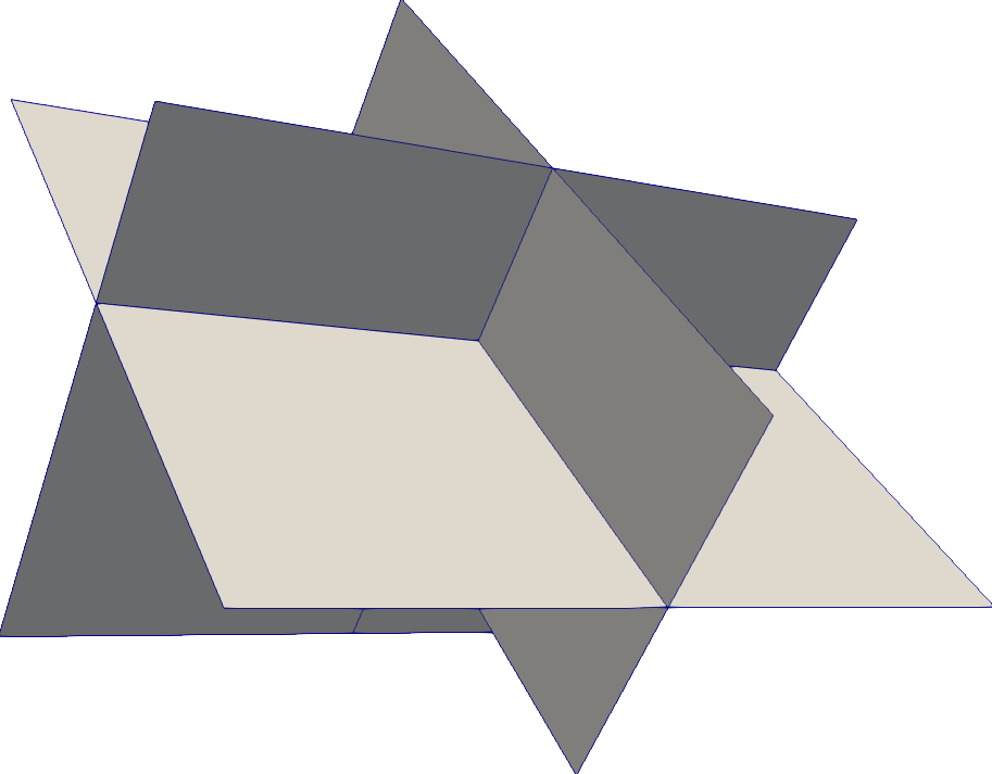
(a) Initial mesh

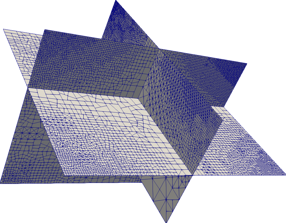
(b) Step 25 MaxMom refinement Order 1

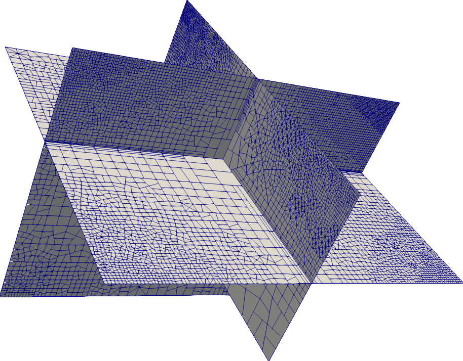
(c) Step 25 TrDir refinement Order 1

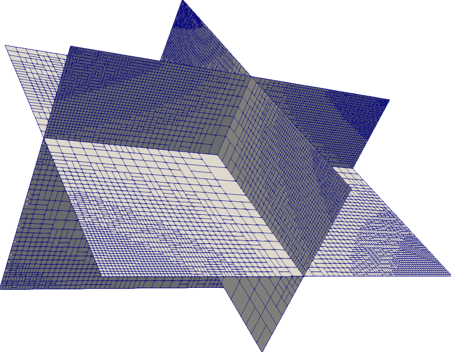
(d) Step 25 MaxEdg refinement Order 1

Figure 4: Problem 2: DFN with meshes at refining step 25

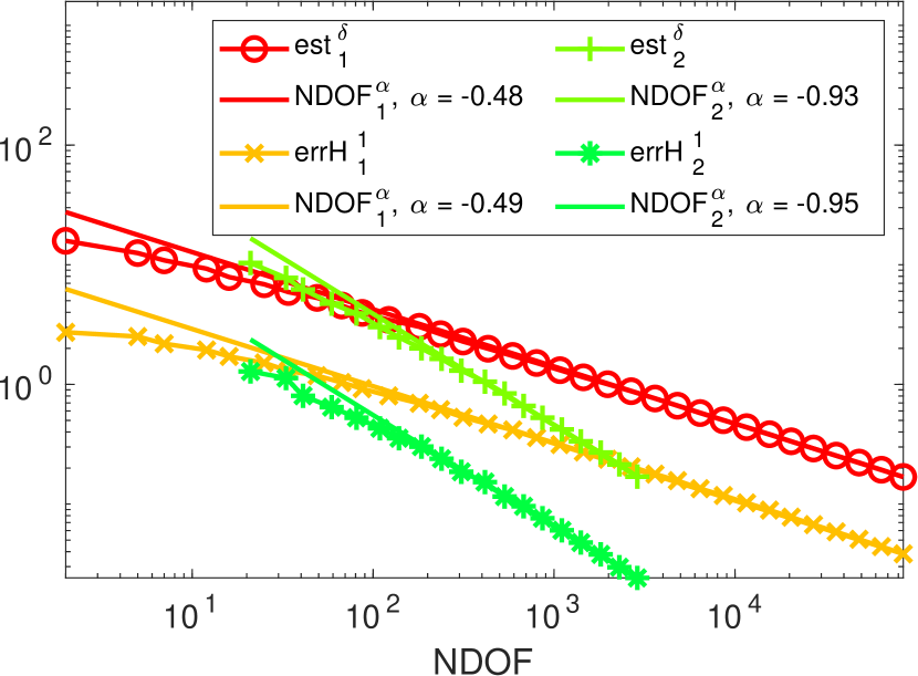
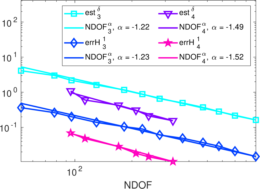
Figure 5: Problem 2: Rates of convergence ($\alpha$) for error and estimator with MaxMom refinement.

TypeRef	Order 1	Order 2	Order 3	Order 4
MaxMom	$\alpha=-0.48$	$\alpha=-0.93$	$\alpha=-1.22$	$\alpha=-1.49$
	$\alpha_{err}=-0.49$	$\alpha_{err}=-0.95$	$\alpha_{err}=-1.23$	$\alpha_{err}=-1.52$
TrDir	$\alpha=-0.49$	$\alpha=-0.95$	$\alpha=-1.14$	$\alpha=-1.49$
	$\alpha_{err}=-0.49$	$\alpha_{err}=-0.92$	$\alpha_{err}=-1.20$	$\alpha_{err}=-1.52$
MaxEdg	$\alpha=-0.49$	$\alpha=-0.92$	$\alpha=-1.32$	$\alpha=-1.47$
	$\alpha_{err}=-0.47$	$\alpha_{err}=-0.94$	$\alpha_{err}=-1.35$	$\alpha_{err}=-1.68$

Table 5: Problem 2: Rates of convergence for the estimator ($\alpha$) and the error ($\alpha_{err}$) with refinement criteria MaxMom, TrDir and MaxEdg.

Step	$\#$ Cells	NDOF	$\varepsilon$	PCG-It
1	12	2	0.0296	1
5	30	16	0.0472	6
10	114	87	0.0541	13
15	455	432	0.0552	25
20	1875	1979	0.0557	55
25	7752	8622	0.0552	114
30	32221	36261	0.0531	234
32	57076	64484	0.0520	309

Table 6: Problem 2: MaxMom refinement Order 1.

Step	$\#$ Cells	NDOF	$\varepsilon$	PCG-It
1	12	2	0.0296	1
5	30	16	0.0441	5
10	113	92	0.0500	13
15	433	428	0.0531	32
20	1741	1933	0.0596	77
25	7047	8221	0.0581	152
30	28933	34475	0.0574	411
33	67557	80552	0.0562	542

Table 7: Problem 2: TrDir refinement Order 1.

Step	$\#$ Cells	NDOF	$\varepsilon$	PCG-It
1	12	2	0.0296	1
5	30	16	0.0476	6
10	113	89	0.0555	12
15	450	418	0.0578	24
20	1847	1885	0.0614	55
25	7737	8203	0.0636	114
30	32385	34978	0.0679	243
31	43231	47014	0.0681	286

Table 8: Problem 2: MaxEdg refinement Order 1.

The geometry and the parameters of this test problem are described in detail in [9, Section 6.1]. The DFN is composed by three fractures and three traces, defined as

$\displaystyle F_{1}$ $\displaystyle=\left(-1,\frac{1}{2}\right)\!\times\!\left(-1,1\right)\!\times\!\{0\}\,,$ $\displaystyle F_{2}$ $\displaystyle=(-1,0)\!\times\!\{0\}\!\times\!(-1,1)\,,$ $\displaystyle F_{3}$ $\displaystyle=\left\{\frac{1}{2}\right\}\!\times\!(-1,1)\!\times\!(-1,1)\,,$

$\displaystyle\Gamma_{1}$ $\displaystyle=F_{1}\cap F_{2}=\left(-1,\frac{1}{2}\right)\!\times\!\{0\}\!\times\!\{0\}\,,$ $\displaystyle\Gamma_{2}$ $\displaystyle=F_{1}\cap F_{3}=\left(-1,0\right)\!\times\!\{0\}\!\times\!\left(-1,1\right)\,,$ $\displaystyle\Gamma_{3}$ $\displaystyle=F_{2}\cap F_{3}=\left\{-\frac{1}{2}\right\}\!\times\!\{0\}\!\times\!(-1,1)\,.$

The chosen exact solution is defined on each fracture as follows:

$$h_{1}(x,y,z) =-\frac{1}{10}\left(x+\frac{1}{2}\right)\left(8xy\left(x^{2}+y^{2}\right)\mathrm{arctan2}(y,x)+x^{3}\right)\,,$$

$$h_{2}(x,y,z) =-\frac{1}{10}\left(x+\frac{1}{2}\right)x^{3}\left(1-8\pi\left\lvert{z}\right\rvert\right)\,,$$

$$h_{3}(x,y,z) =y(y-1)(y+1)(z-1)z\,,$$

and all fractures have transmissivities set to $1$.

In Figure 4, we report some of the meshes generated by the refinement process. Similarly to the previous test, a refinement is induced also far from traces due to the presence of a non-null forcing term.

In Figure 5 we report the rates of convergence ($\alpha$) of the error and of the error estimator considering the strategy MaxMom. The rates of convergence for the strategies MaxMom, TrDir and MaxEdg are shown in the Table 5. The convergence rates are computed on the basis of the last five refinement iterations: again we can remark a very good agreement between the error and the estimator. The sub-optimal rates of convergence with higher VEM orders is still due to the bounded regularity of the solution.

In Tables 6-8 we report the same quantities reported in Tables 2-4 in order to describe the refinement process. We observe again that the effectivity index is almost independent of the meshsize since, as the mesh starts to have a sufficient number of DOFs, it displays small variations.

7 Numerical Results on a realistic DFN

In this section we discuss the results obtained by the four presented refinement strategies when applied to more realistic DFNs. The geometry of the considered DFNs is fixed and is composed by 86 fractures and 159 traces, with a maximum number of traces per fracture equal to 11 and a mean value of traces per fracture equal to 1.85, see Figure 6. We consider two test cases where the transmissivities of the fractures are sampled from two log-normal distributions having standard deviations equal to $10$ and $10^{4}$, respectively. These two problems are tagged with the labels DFN86E01 and DFN86E04.

The problems considered have no forcing terms, and the flux is driven by the presence of two Dirichlet boundary conditions (10 on the boundaries at $x=0$ and 0 at the boundaries at $x=1000$), whereas homogeneous Neumann boundary conditions are imposed on all the other boundaries.

In the following analysis we display the convergence rates of the error estimate with respect to the number of degrees of freedom and we assess how the refinement strategies impact on the aspect ratio of the cells of a selected fracture (Fracture $72$), and on the iterations of the preconditioned conjugate gradient method used to solve the linear system.

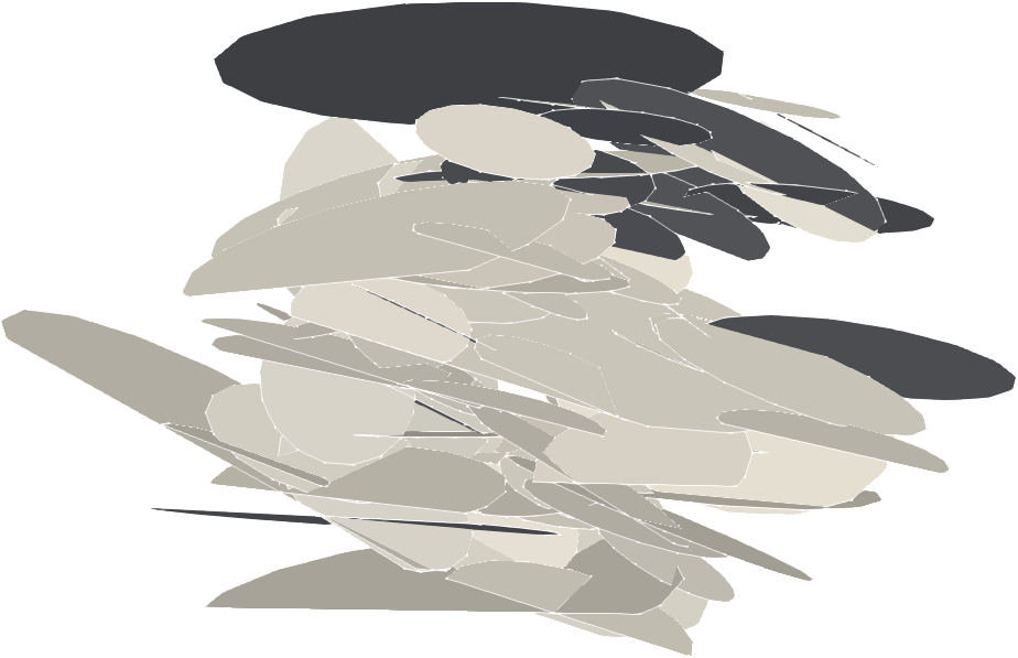
Figure 6: DFN with 86 fractures.

In Figures 7 and 8 we display the behaviour of the estimators with respect to the number of DOFs for the four refinement strategies considered and we report the slope of the estimator for each VEM order, for the two problems. We can observe that all the refinement strategies display an optimal asymptotic rate of convergence up to VEM order 2 ($-0.5$ for the VEM Order 1 and $-1.0$ for the VEM Order 2). For higher VEM orders the bounded regularity constraints the rates of convergence. The trend of the rate of convergence results similar even if the fluxes in the these two DFNs are completely different.

In Figure 9 we plot the behaviour of the ratio PCG-It/NDOF. After the initial noisy behaviour we can observe a decreasing asymptotical trend for all the considered refinement strategies. These plots highlight the advantages of a suitably refined mesh also on the performances of the linear solver.

In Figure 10 we report the minimal mesh on Fracture 72: this is the common initial mesh for all the refinement strategies and for both DFN86E01 and DFN86E04. In Figures 11 and 12 we display the meshes produced by all the considered refinement strategies. The TrDir strategy produces a stronger and sharper refinement along the traces. The switch from TrDir to MaxMom for elements with an aspect ratio over MaxAR prevents the generation of badly shaped elements parallel to the traces. The MaxPnt strategy produces a mesh quite similar to the mesh produced by MaxMom due to the fact that we fave few cells with a number of vertices larger than MaxNP during the refinement process. In Figures 13 and 14 we report the minimum, the mean and the maximum aspect ratios of the cells on Fracture 72 along the refinement process. We remark that in all the strategies we use MaxMom strategy to refine the elements with large aspect ratio. The MaxMom and the MaxEdg strategies produce a decreasing mean aspect ratio, whereas TrDir and MaxPnt have a different behaviour. A slight difference from the two figures can be seen in the TrDir plots. The average AR grows in the DFN86E04 test case because the MaxMom strategy is less used due to the weaker refinement around the traces due to the different transmissivities on the intersecting fractures that justify a smaller flux (notice the more coarse mesh for DFN86E04 comparing Figures 11 and 12).

(a) MaxMom refinement.

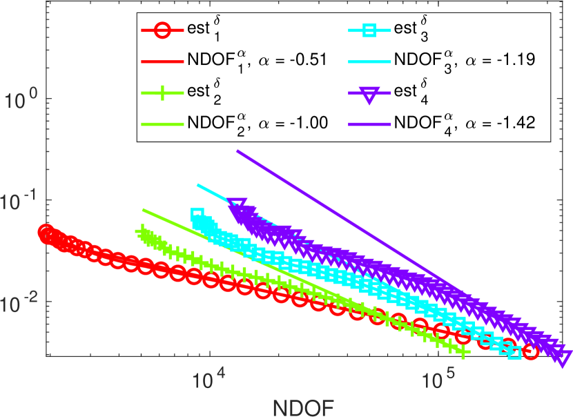
(b) TrDir refinement.

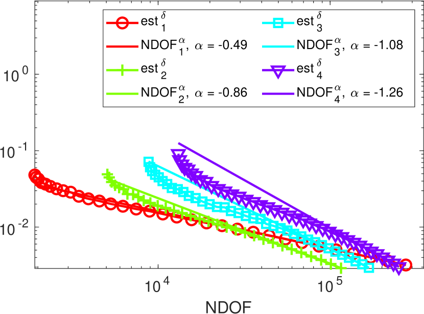
(c) MaxPnt refinement.

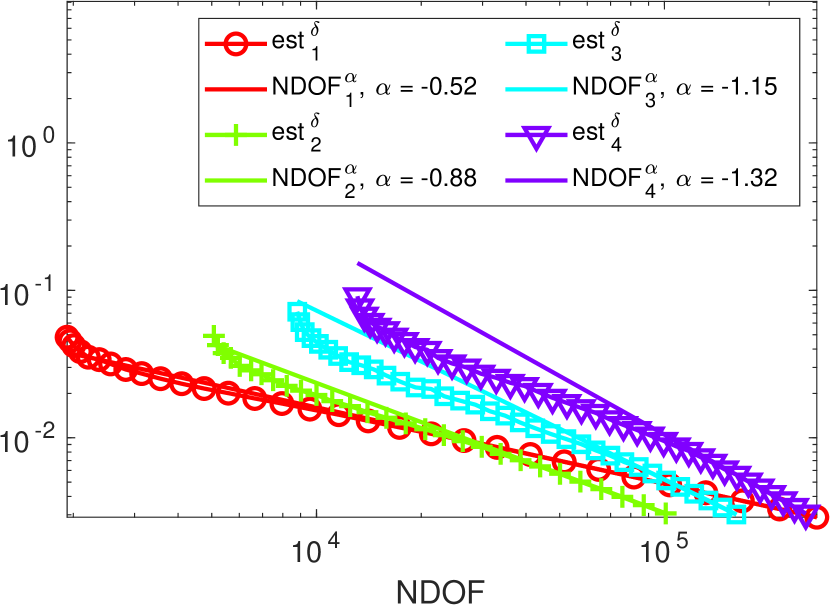
(d) MaxEdg refinement.

Figure 7: DFN86E01: Estimator vs. NDOF

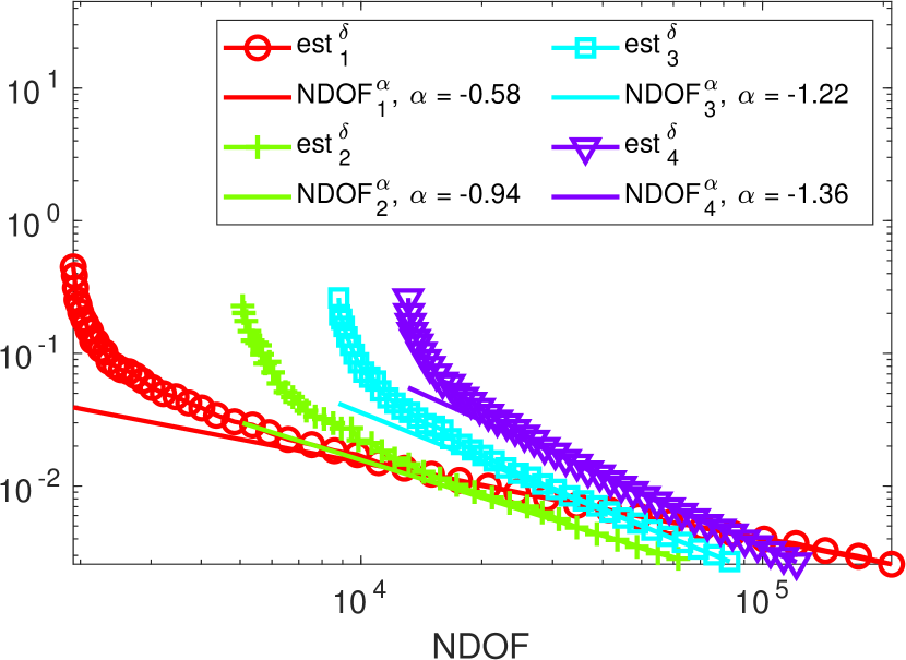
(a) MaxMom refinement.

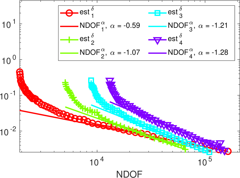
(b) TrDir refinement.

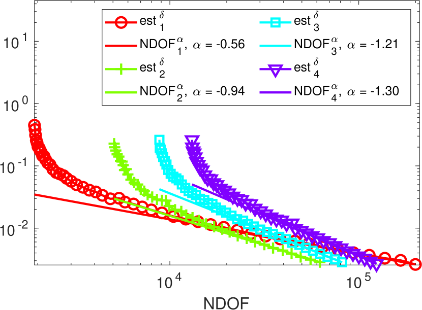
(c) MaxPnt refinement.

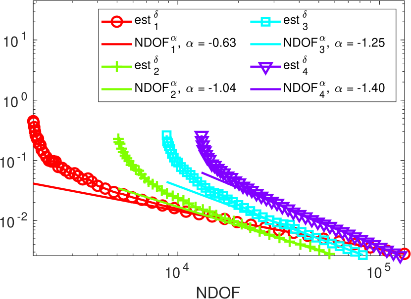
(d) MaxEdg refinement.

Figure 8: DFN86E04: Estimator vs. NDOF

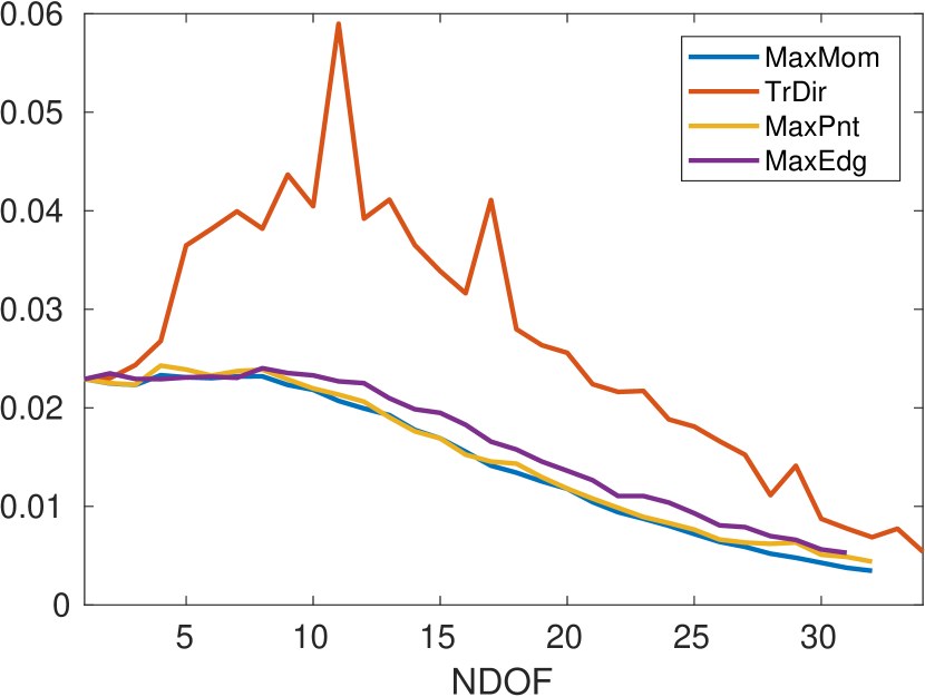
(a) DFN86E01

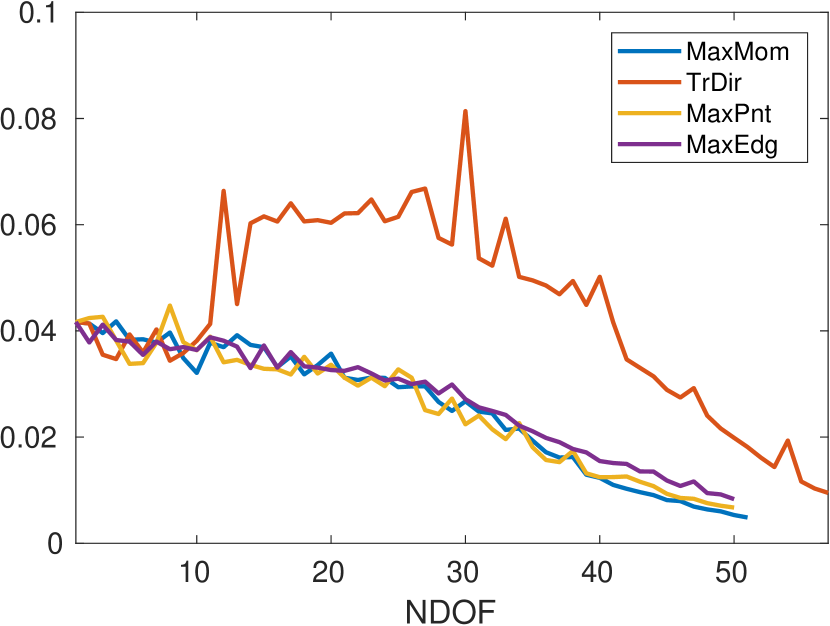
(b) DFN86E04

Figure 9: Ratio between PCG-It and NDOF

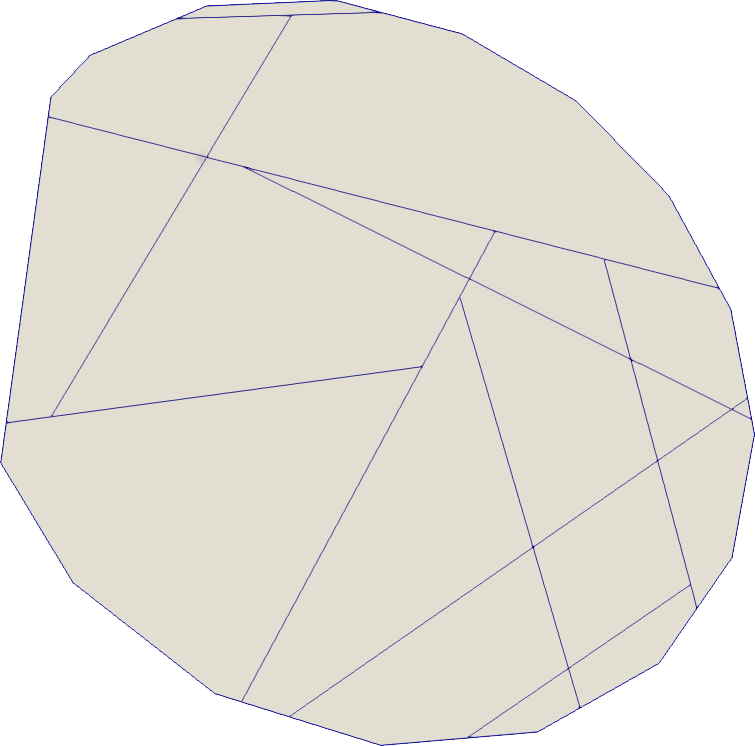
Figure 10: DFN86E01 - DFN86E04: initial mesh on Fracture 72.

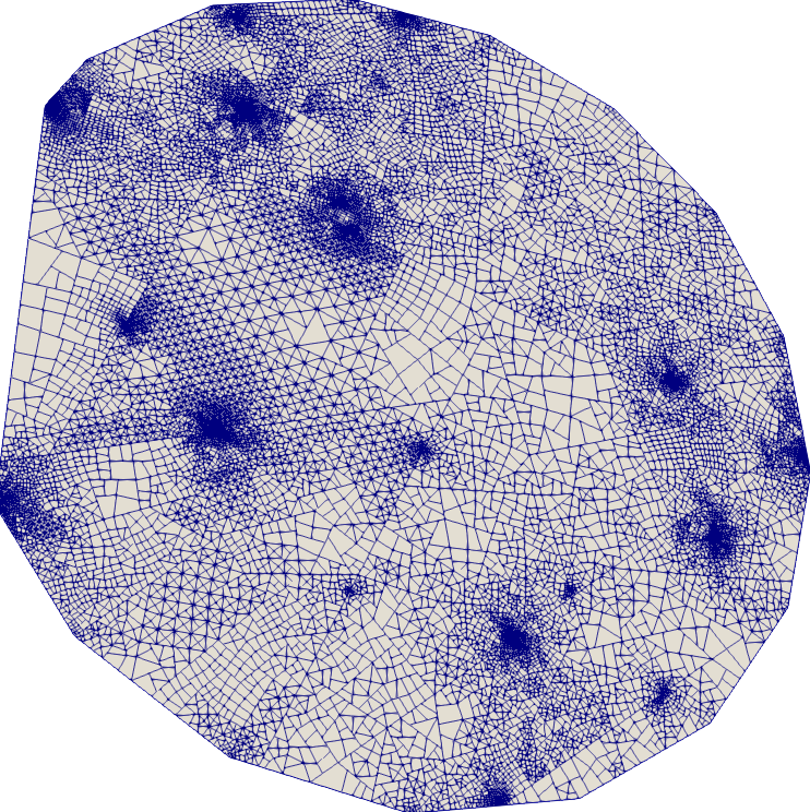
(a) MaxMom refinement.

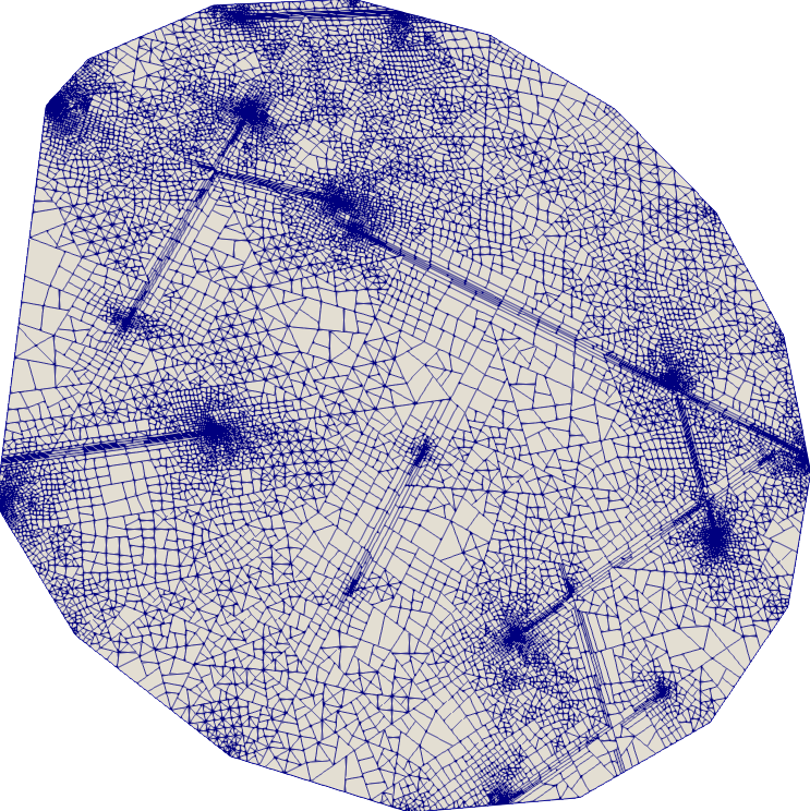
(b) TrDir refinement.

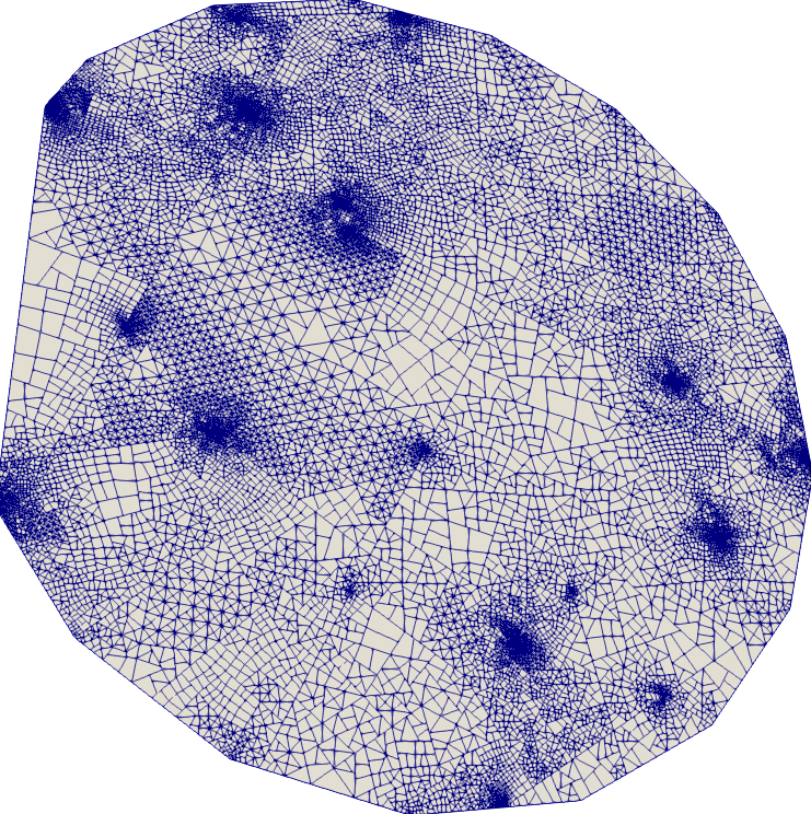
(c) MaxPnt refinement.

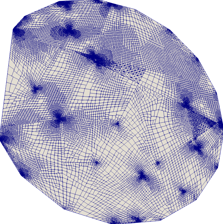
(d) MaxEdg refinement.

Figure 11: DFN86E01: final mesh on Fracture 72.

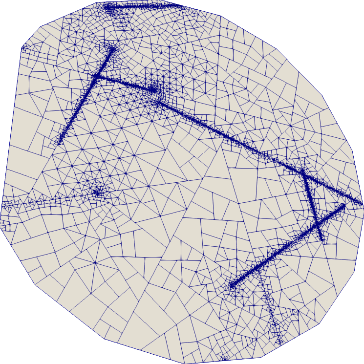
(a) MaxMom refinement.

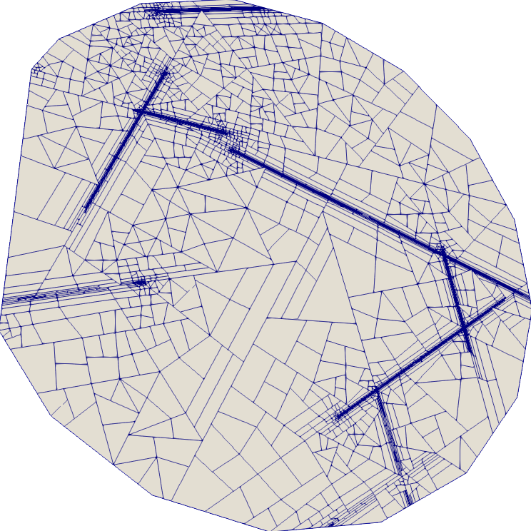
(b) TrDir refinement.

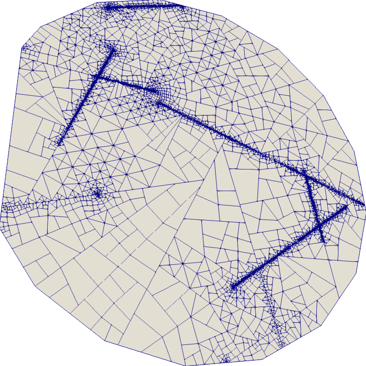
(c) MaxPnt refinement.

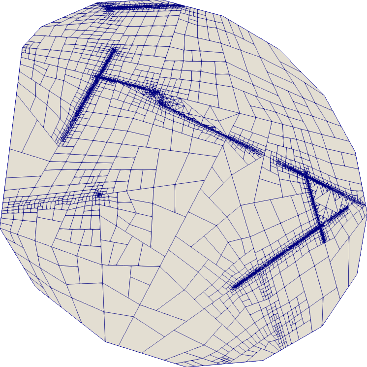
(d) MaxEdg refinement.

Figure 12: DFN86E04: final mesh on Fracture 72.

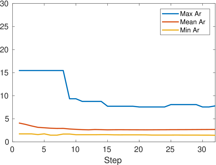
(a) MaxMom refinement.

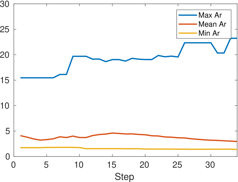
(b) TrDir refinement.

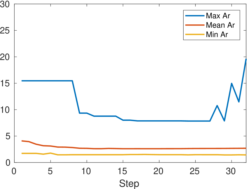
(c) MaxPnt refinement.

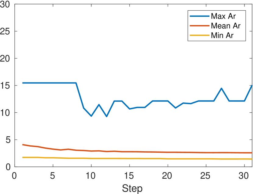
(d) MaxEdg refinement.

Figure 13: DFN86E01: aspect ratio statistics of the mesh on Fracture 72.

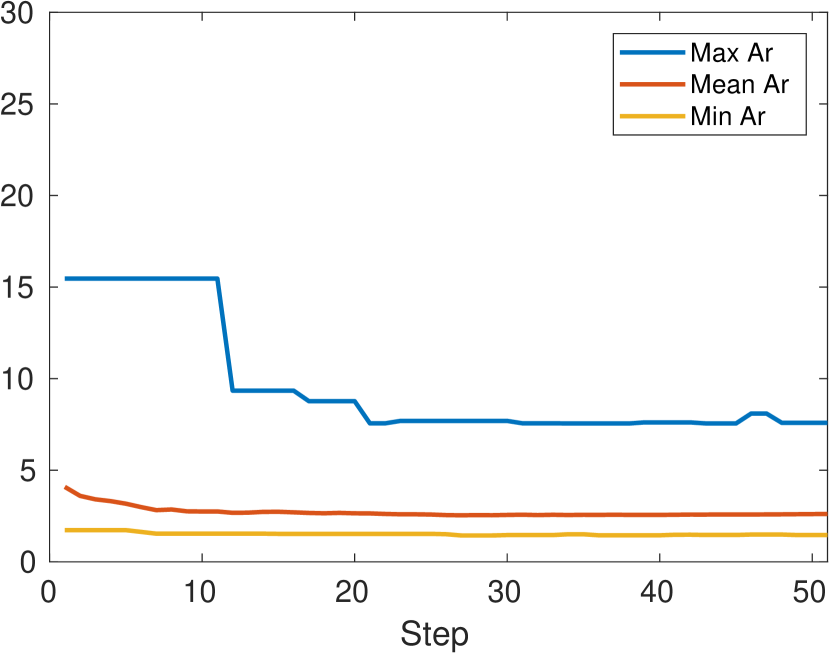
(a) MaxMom refinement.

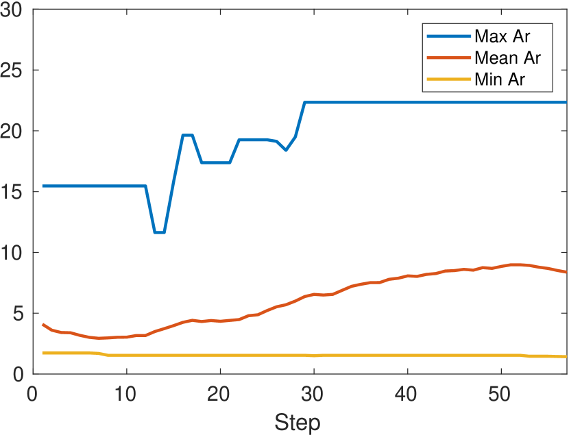
(b) TrDir refinement.

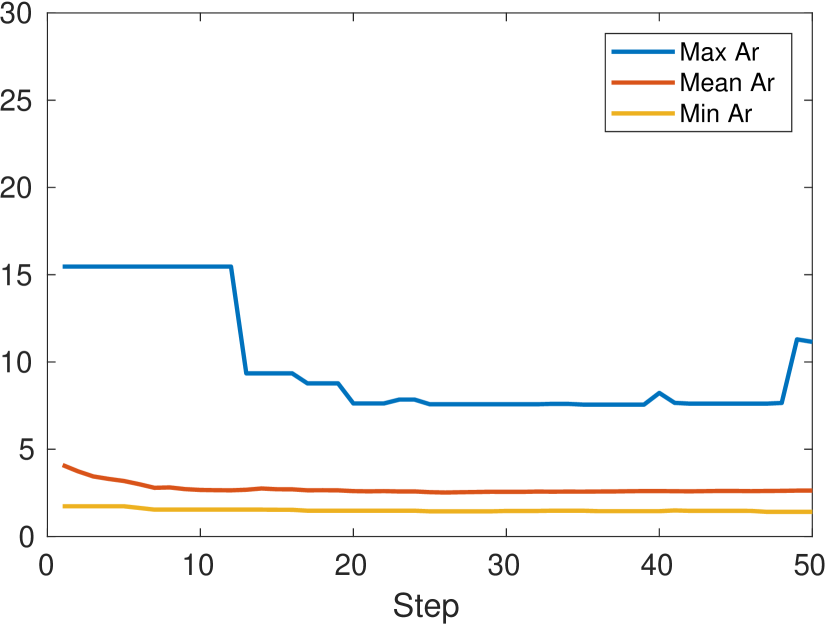
(c) MaxPnt refinement.

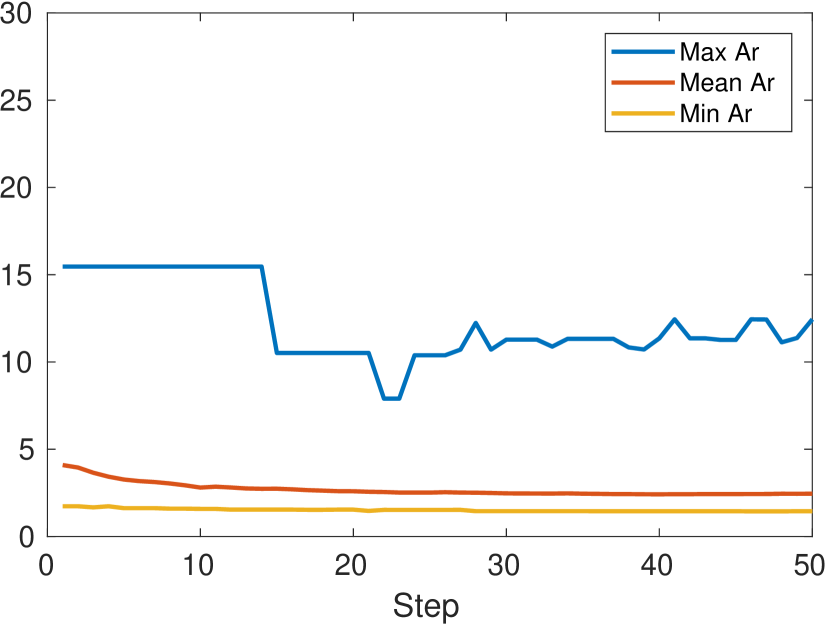
(d) MaxEdg refinement.

Figure 14: DFN86E04: aspect ratio statistics of the mesh on Fracture 72.

References

- [1] , . Eigen conjugate gradient. http://eigen.tuxfamily.org/dox/classEigen_1_1ConjugateGradient.html. Accessed: 12-09-2019.
- Ahmad et al. [2013] Ahmad, B., Alsaedi, A., Brezzi, F., Marini, L.D., Russo, A., 2013. Equivalent projectors for virtual element methods. Computers & Mathematics with Applications 66, 376–391.
- Ahmed et al. [2017] Ahmed, R., Edwards, M.G., Lamine, S., Huisman, B.A., Pal, M., 2017. CVD-MPFA full pressure support, coupled unstructured discrete fracture matrix darcy-flux approximations. Journal of Computational Physics 349, 265 – 299.
- Al-Hinai et al. [2017] Al-Hinai, O., Wheeler, M.F., Yotov, I., 2017. A generalized mimetic finite difference method and two-point flux schemes over voronoi diagrams. ESAIM: Mathematical Modelling and Numerical Analysis 51, 679–706.
- [5] Antonietti, P.F., Berrone, S., Borio, A., D’Auria, A., Verani, M., Weisser, S., . Anisotropic a posteriori error estimate for the virtual element method. In preparation.
- Antonietti et al. [2016] Antonietti, P.F., Formaggia, L., Scotti, A., Verani, M., Verzott, N., 2016. Mimetic finite difference approximation of flows in fractured porous media. ESAIM: M2AN 50, 809–832. doi:10.1051/m2an/2015087.
- Beirão da Veiga et al. [2013] Beirão da Veiga, L., Brezzi, F., Cangiani, A., Manzini, G., Marini, L.D., Russo, A., 2013. Basic principles of virtual element methods. Mathematical Models and Methods in Applied Sciences 23, 199–214. URL: http://www.worldscientific.com/doi/abs/10.1142/S0218202512500492, doi:10.1142/S0218202512500492.
- Beirão da Veiga et al. [2015] Beirão da Veiga, L., Brezzi, F., Marini, L.D., Russo, A., 2015. Virtual element methods for general second order elliptic problems on polygonal meshes. Mathematical Models and Methods in Applied Sciences 26, 729–750. doi:10.1142/S0218202516500160.
- Benedetto et al. [2016a] Benedetto, M., Berrone, S., Borio, A., Pieraccini, S., Scialò, S., 2016a. A hybrid mortar virtual element method for discrete fracture network simulations. J. Comput. Phys. 306, 148–166. doi:10.1016/j.jcp.2015.11.034.
- Benedetto et al. [2014] Benedetto, M., Berrone, S., Pieraccini, S., Scialò, S., 2014. The virtual element method for discrete fracture network simulations. Comput. Methods Appl. Mech. Engrg. 280, 135 – 156. doi:10.1016/j.cma.2014.07.016.
- Benedetto et al. [2016b] Benedetto, M., Berrone, S., Scialò, S., 2016b. A globally conforming method for solving flow in discrete fracture networks using the virtual element method. Finite Elem. Anal. Des. 109, 23–36. doi:10.1016/j.finel.2015.10.003.
- Benedetto et al. [2017] Benedetto, M.F., Borio, A., Scialò, S., 2017. Mixed virtual elements for discrete fracture network simulations. Finite Elements in Analysis & Design 134, 55–67. doi:10.1016/j.finel.2017.05.011.
- Berrone and Borio [2017a] Berrone, S., Borio, A., 2017a. Orthogonal polynomials in badly shaped polygonal elements for the Virtual Element Method. Finite Elements in Analysis & Design 129, 14–31. doi:10.1016/j.finel.2017.01.006.
- Berrone and Borio [2017b] Berrone, S., Borio, A., 2017b. A residual a posteriori error estimate for the virtual element method. Mathematical Models and Methods in Applied Sciences 27, 1423–1458. URL: http://www.worldscientific.com/doi/abs/10.1142/S0218202517500233, doi:10.1142/S0218202517500233.
- Berrone et al. [2016] Berrone, S., Borio, A., Scialò, S., 2016. A posteriori error estimate for a PDE-constrained optimization formulation for the flow in DFNs. SIAM J. Numer. Anal. 54, 242–261. doi:10.1137/15M1014760.
- Berrone et al. [2019a] Berrone, S., Borio, A., Vicini, F., 2019a. Reliable a posteriori mesh adaptivity in discrete fracture network flow simulations. Computer Methods in Applied Mechanics and Engineering 354, 904 – 931. URL: http://www.sciencedirect.com/science/article/pii/S0045782519303470, doi:10.1016/j.cma.2019.06.007.
- Berrone et al. [2015] Berrone, S., Canuto, C., Pieraccini, S., Scialò, S., 2015. Uncertainty quantification in discrete fracture network models: stochastic fracture transmissivity. Comput. Math. Appl. 70, 603–623. doi:10.1016/j.camwa.2015.05.013.
- Berrone et al. [2018] Berrone, S., Canuto, C., Pieraccini, S., Scialò, S., 2018. Uncertainty quantification in discrete fracture network models: Stochastic geometry. Water Resources Research 54, 1338–1352. URL: https://agupubs.onlinelibrary.wiley.com/doi/abs/10.1002/2017WR021163, doi:10.1002/2017WR021163.
- Berrone et al. [2019b] Berrone, S., D’Auria, A., Vicini, F., 2019b. Fast and robust flow simulations in discrete fracture networks with GPGPUs. GEM - International Journal on Geomathematics 10, 8.
- Berrone et al. [2014a] Berrone, S., Fidelibus, C., Pieraccini, S., Scialò, S., 2014a. Simulation of the steady-state flow in discrete fracture networks with non-conforming meshes and extended finite elements. Rock Mechanics and Rock Engineering 47, 2171–2182. doi:10.1007/s00603-013-0513-5.
- Berrone et al. [2013a] Berrone, S., Pieraccini, S., Scialò, S., 2013a. On simulations of discrete fracture network flows with an optimization-based extended finite element method. SIAM J. Sci. Comput. 35, A908–A935. URL: http://dx.doi.org/10.1137/120882883, doi:10.1137/120882883.
- Berrone et al. [2013b] Berrone, S., Pieraccini, S., Scialò, S., 2013b. A PDE-constrained optimization formulation for discrete fracture network flows. SIAM J. Sci. Comput. 35, B487–B510. doi:10.1137/120865884.
- Berrone et al. [2014b] Berrone, S., Pieraccini, S., Scialò, S., 2014b. An optimization approach for large scale simulations of discrete fracture network flows. J. Comput. Phys. 256, 838–853. doi:10.1016/j.jcp.2013.09.028.
- Berrone et al. [2019c] Berrone, S., Scialò, S., Vicini, F., 2019c. Parallel meshing, discretization and computation of flow in massive Discrete Fracture Networks. SIAM J. Sci. Comput. 41, C317–C338. doi:10.1137/18M1228736.
- Brenner et al. [2017] Brenner, K., Hennicker, J., Masson, R., Samier, P., 2017. Gradient discretization of hybrid-dimensional darcy flow in fractured porous media with discontinuous pressures at matrix fracture interfaces. IMA Journal of Numerical Analysis 37, 1551–1585.
- Cacas et al. [1990] Cacas, M.C., Ledoux, E., de Marsily, G., Tillie, B., Barbreau, A., Durand, E., Feuga, B., Peaudecerf, P., 1990. Modeling fracture flow with a stochastic discrete fracture network: calibration and validation: 1. the flow model. Water Resour. Res. 26, 479–489. doi:10.1029/WR026i003p00479.
- Beirão Da Veiga et al. [2017] Beirão Da Veiga, L., Lovadina, C., Russo, A., 2017. Stability analysis for the virtual element method. Mathematical Models and Methods in Applied Sciences 27, 2557–2594. URL: www.scopus.com.
- Dershowitz and Einstein [1988] Dershowitz, W.S., Einstein, H.H., 1988. Characterizing rock joint geometry with joint system models. Rock Mechanics and Rock Engineering 1, 21–51.
- Dershowitz and Fidelibus [1999] Dershowitz, W.S., Fidelibus, C., 1999. Derivation of equivalent pipe networks analogues for three-dimensional discrete fracture networks by the boundary element method. Water Resource Res. 35, 2685–2691. doi:10.1029/1999WR900118.
- Dörfler [1996] Dörfler, W., 1996. A convergent adaptive algorithm for poisson’s equation. SIAM Journal on Numerical Analysis 33, 1106–1124.
- Fidelibus et al. [2009] Fidelibus, C., Cammarata, G., Cravero, M., 2009. Hydraulic characterization of fractured rocks. In: Abbie M, Bedford JS (eds) Rock mechanics: new research. Nova Science Publishers Inc., New York.
- Flemisch et al. [2018] Flemisch, B., Berre, I., Boon, W., Fumagalli, A., Schwenck, N., Scotti, A., Stefansson, I., Tatomir, A., 2018. Benchmarks for single-phase flow in fractured porous media. Advances in Water Resources 111, 239–258.
- Formaggia et al. [2014] Formaggia, L., Antonietti, P., Panfili, P., Scotti, A., Turconi, L., Verani, M., Cominelli, A., 2014. Optimal techniques to simulate flow in fractured reservoir, in: ECMOR XIV-14th European conference on the mathematics of oil recovery.
- Fourno et al. [2019] Fourno, A., Ngo, T.D., Noetinger, B., Borderie, C.L., 2019. Frac: A new conforming mesh method for discrete fracture networks. Journal of Computational Physics 376, 713 – 732. URL: http://www.sciencedirect.com/science/article/pii/S0021999118306624, doi:10.1016/j.jcp.2018.10.005.
- Fumagalli et al. [2019] Fumagalli, A., Keilegavlen, E., Scialò, S., 2019. Conforming, non-conforming and non-matching discretization couplings in discrete fracture network simulations. J. Comput. Phys. 376, 694–712. doi:10.1016/j.jcp.2018.09.048.
- Fumagalli and Scotti [2013] Fumagalli, A., Scotti, A., 2013. A numerical method for two-phase flow in fractured porous media with non-matching grids. Advances in Water Resources 62, 454 – 464. doi:10.1016/j.advwatres.2013.04.001.
- Fumagalli and Scotti [2014] Fumagalli, A., Scotti, A., 2014. An efficient xfem approximation of darcy flows in arbitrarily fractured porous media. Oil Gas Sci. Technol. – Rev. IFP Energies nouvelles 69, 555–564. doi:10.2516/ogst/2013192.
- Garipov et al. [2016] Garipov, T.T., Karimi-Fard, M., Tchelepi, H.A., 2016. Discrete fracture model for coupled flow and geomechanics. Computational Geosciences 20, 149–160.
- Hyman et al. [2014] Hyman, J., Gable, C., Painter, S., Makedonska, N., 2014. Conforming delaunay triangulation of stochastically generated three dimensional discrete fracture networks: A feature rejection algorithm for meshing strategy. SIAM Journal on Scientific Computing 36, A1871–A1894. doi:10.1137/130942541.
- Jaffré and Roberts [2012] Jaffré, J., Roberts, J.E., 2012. Modeling flow in porous media with fractures; discrete fracture models with matrix-fracture exchange. Numerical Analysis and Applications 5, 162–167.
- Karimi-Fard and Durlofsky [2014] Karimi-Fard, M., Durlofsky, L.J., 2014. Unstructured adaptive mesh refinement for flow in heterogeneous porous media, in: ECMOR XIV-14th European conference on the mathematics of oil recovery. doi:10.3997/2214-4609.20141856.
- Lenti and Fidelibus [2003] Lenti, V., Fidelibus, C., 2003. A bem solution of steady-state flow problems in discrete fracture networks with minimization of core storage. Computers & Geosciences 29, 1183 – 1190. doi:10.1016/S0098-3004(03)00140-7.
- Ngo et al. [2017] Ngo, T.D., Fourno, A., Noetinger, B., 2017. Modeling of transport processes through large-scale discrete fracture networks using conforming meshes and open-source software. Journal of Hydrology 554, 66 – 79. URL: http://www.sciencedirect.com/science/article/pii/S0022169417305899, doi:10.1016/j.jhydrol.2017.08.052.
- Noetinger [2015] Noetinger, B., 2015. A quasi steady state method for solving transient darcy flow in complex 3d fractured networks accounting for matrix to fracture flow. Journal of Computational Physics 283, 205 – 223.
- Pichot et al. [2010] Pichot, G., Erhel, J., de Dreuzy, J., 2010. A mixed hybrid mortar method for solving flow in discrete fracture networks. Applicable Analysis 89, 1629 – 643. doi:10.1080/00036811.2010.495333.
- Pichot et al. [2012] Pichot, G., Erhel, J., de Dreuzy, J., 2012. A generalized mixed hybrid mortar method for solving flow in stochastic discrete fracture networks. SIAM Journal on scientific computing 34, B86 – B105. doi:10.1137/100804383.
- Beirão da Veiga et al. [2014] Beirão da Veiga, L., Brezzi, F., Marini, L.D., Russo, A., 2014. The hitchhiker’s guide to the virtual element method. Mathematical Models and Methods in Applied Sciences 24, 1541–1573. URL: https://doi.org/10.1142/S021820251440003X, doi:10.1142/S021820251440003X.