NNLO QED contribution to the $\mu e\to\mu e$ elastic scattering

Abstract

We present the current status of the Next-to-Next-to-Leading Order QED contribution to the $\mu e$-scattering. Particular focus is given to the techniques involved to tackle the virtual amplitude and their automatic implementation. Renormalization of the amplitude will be also discuss in details.

1 Introduction

The current measurements of the muon anomalous magnetic moment $a_{\mu}=(g_{\mu}-2)/2$ indicate a discrepancy of $\sim 3.5\sigma$ from the Standard Model prediction (blum2013muon, ). This fact might be a hint of new physics. New upcoming experiments at Fermilab and J-PARC will improve significantly the precision of $a_{\mu}^{exp}$, hence higher accuracy for $a_{\mu}^{th}$ from the theoretical side is required.

A very clean way to achieve the aimed precision involves the determination of the leading hadronic contribution $\Delta\alpha^{\text{had}}(q^{2})$ to the electromagnetic coupling in the space-like region (Carloni_Calame_2015, ; Abbiendi_2017, ). The MUonE experiment, recently proposed at the CERN, is meant to obtain an estimation of $\Delta\alpha^{\text{had}}(q^{2})$ through a measurement of the differential cross section of the $\mu e$-elastic scattering. In order to be competitive with the time-like datas, a precision of 10ppm is required, both on statistical and systematic errors.

QED contributions to $\mu e$-elastic scattering constitute an irreducible background for the measurement, and they represent a relevant source of systematic errors; results for Leading Order (LO) and Next-to-Leading Order (NLO) corrections are already available (Alacevich:2018vez, ), as well as the Next-to-Next-to-Leading Order (NNLO) hadronic ones (Fael:2018dmz, ; Fael:2019nsf, ). However, Next-to-Next-to-Leading Order (NNLO) corrections to $\mu e$-elastic scattering are mandatory to achieve the 10ppm precision.

In this work, we summarize the current status of the double-virtual contributions to the NNLO QED $\mu e$-elastic scattering. The review is organized as follows: Section 2 recaps the external kinematic definitions we use for characterizing the $\mu e$-elastic scattering; Section 3 states the basics of the calculation process, stressing the importance of the Feynman integrals. The next sessions will present the heart of this calculation: the decomposition of the amplitude and the evaluation of the master integrals.

The decomposition strategies are presented in Section 4. We discuss the main features of the Adaptive Integrand Decomposition (Mastrolia_2016, ; mastrolia2016adaptive, ) and its implementation Aida (primophdth, ; torresphdth, ), and the Integral Reduction algorithms involving the Integration-by-parts identities Chetyrkin:1981qh ; Laporta_2000 ; manteuffel2012reduze ; Maierhoefer:2017hyi . These method are exploit to obtain a reduction of the full amplitude in terms of a minimal set of master integrals. Section 5 is focused on the evaluation approaches, presenting the analytical and the numerical ways. Analytical strategy is based on solving systems of differential equations (Barucchi_1973, ; Kotikov:1990kg, ; Remiddi:1997ny, ; Gehrmann_2000, ) which master integrals obey. The main results of the analytical method for the $\mu e$-elastic scattering are collected into (Mastrolia_2017, ; Di_Vita_2018, ), and cross-checked numerically. Alternatively, a numerical method which can be userful in these calculation is the so-called sector decomposition (HEINRICH_2008, ), which will be briefly introduced.

Section 6 is devoted to present the complete Mathematica implementation which embeds each step of the calculation, from the generation of the amplitude to evaluation of the master integrals. A flowchart of the global algorithm is presented in Fig. 2.

In Section 7 we define the renormalization procedure which will be adopted to obtain a UV finite $\mu e$-elastic Scattering Amplitude. Both $\overline{\text{MS}}$ and on-shell schemes are employed to renormalize respectively the QED coupling constant and the muon fermion field and mass.

Lastly, we present the main result achieved for the $\mu e$-elastic scattering and we point out the next steps needed to complete the full NNLO contribution.

2 $\mu e$-elastic Scattering process

The process under investigation is the elastic scattering

$$\mu^{+}(p_{1})e^{-}(p_{2})\to e^{-}(-p_{3})\mu^{+}(-p_{4}),$$ (1)

where $p_{i}$ are the on-shell momenta: $p_{1}^{2}=p_{4}^{2}=m_{\mu}^{2}$ and $p_{2}^{2}=p_{3}^{2}=m_{e}^{2}$. Let $p_{4}$ be the dependent momentum. From the general Mandelstam variables definition, $s_{ij}=(p_{i}+p_{j})^{2}$, define

$$\begin{gathered}s=s_{12},\quad t=s_{23},\quad u=s_{13},\\ s+t+u=2m_{e}^{2}+2m_{\mu}^{2}.\end{gathered}$$ (2)

The physical phase-space region is constrained by the following conditions

$$\begin{gathered}s\geq(m_{e}+m_{\mu})^{2},\\ -\frac{\lambda(s,m_{\mu}^{2},m_{e}^{2})}{s}<t<0,\\ \begin{aligned} \lambda(s,m_{\mu}^{2},m_{e}^{2})\leavevmode\nobreak\ =\leavevmode\nobreak\ &s^{2}+(m_{\mu}^{2})^{2}+(m_{e}^{2})^{2}-2sm_{\mu}^{2}\\ &-2sm_{e}^{2}-2m_{e}^{2}m_{\mu}^{2}.\end{aligned}\end{gathered}$$ (3)

The ratio between electron and muon mass is of the order $10^{-5}$. This enforce the validity of the massless electron approximation, which yields many advantages to the NNLO calculation. Therefore, from now on we set $m_{e}=0$ and $m_{\mu}=m$.

3 Double-virtual contributions

Within the perturbative QFT approach, the QED cross section $\sigma$ of the $e\mu$-scattering is a series expansion in terms of the coupling constant $\alpha$,

$$\sigma=\sigma_{LO}+\sigma_{NLO}+\sigma_{NNLO}+\cdots+\mathcal{O}(\alpha^{2+n}).$$ (4)

For $2\to 2$ scattering process, $\sigma$ is also related to the Feynman amplitude $\mathcal{M}$ through the well-known relation

$$\sigma=C_{\text{flux}}\int|\mathcal{M}|^{2}d\text{PS}_{2},$$ (5)

where $C_{\text{flux}}$ is the flux factor and $d\text{PS}_{2}$ is the infinitesimal phase-space element. Matching Eq. (4) and (5), the order-by-order expression of $\sigma$ is manifest,

$$\sigma_{LO}\sim \leavevmode\nobreak\ |\mathcal{M}_{0}|^{2},$$ (6)

$$\sigma_{NLO}\sim \leavevmode\nobreak\ 2\text{Re}[\mathcal{M}_{0}^{*}\mathcal{M}_{1l}]+|\mathcal{M}_{\text{r}}|^{2},$$

$$\sigma_{NNLO}\sim \leavevmode\nobreak\ 2\text{Re}[\mathcal{M}_{0}^{*}\mathcal{M}_{2l}]+2\text{Re}[\mathcal{M}_{1l}^{*}\mathcal{M}_{1l}]$$

$$+2\text{Re}[\mathcal{M}_{r}^{*}\mathcal{M}_{1l,r}]+|\mathcal{M}_{2r}|^{2},$$

where $\mathcal{M}_{0}$ is the Born amplitude, $\mathcal{M}_{1l}$ and $\mathcal{M}_{2l}$ are respectively the one and two-loop Feynman amplitude, $\mathcal{M}_{r}$ and $\mathcal{M}_{2r}$ are the real and the double-real emission amplitudes, with respectively one and two more particles emitted in the final state, and $\mathcal{M}_{1l,r}$ the real-virtual amplitudes, one-loop amplitude with one more particle emitted in the final start.

Figure 1: Two-loop diagrams contributing the QED NNLO amplitude for the $\mu e$-scattering

The double-virtual contribution $\mathcal{M}_{2l}$ to $\sigma_{NNLO}$ (Fig. 1) is a combination of dimensionally regularized Feynman integrals

$$2\text{Re}[\mathcal{M}_{0}^{*}\mathcal{M}_{2l}]=\sum_{\bar{i}}A_{\bar{i}}I_{\overline{i}}(\mathbf{s}),$$ (7)

where the coefficients $A_{\bar{i}}$ depend on the kinematic variables $\mathbf{s}=(s,t,m^{2})$. The Feynman integrals $I_{\overline{i}}(\mathbf{s})$ have the general form

$$I_{\overline{i}}(\mathbf{s})=\int_{\mathbf{k}}\frac{\mathcal{N}_{\bar{i}}(\mathbf{k},\mathbf{s})}{D^{i_{1}}_{1}\cdots D^{i_{n}}_{n}},\quad\bar{i}\in\mathbb{N}^{n},$$ (8)

and depend on the kinematic invariants $\mathbf{s}$ and the dimension $d$. The numerator $\mathcal{N}_{\bar{i}}$ is a general polynomial of the scalar products between loop and external momenta. The denominators $D_{j}$ are inverse scalar propagators, whose form is $D_{j}=q_{j}^{2}(\mathbf{k},\mathbf{p})-m^{2}_{j}$. The multi-index $\bar{i}=(i_{1},\cdots,i_{n})$ contains the exponents of the denominators.

Direct integration of Feynman integrals objects is usually not allowed. A viable way to calculate them efficiently involves decomposition methods: Feynman integrals can be expressed into combinations of "simpler" integrals. Such integrals can be evaluated either analytically of numerically. In the next session, the algorithm employed in the calculation of the amplitude (7) is presented.

4 Decomposing the Amplitude

There exist several decomposition methods, which can be apply either to integrands (Ossola_2007, ; Mastrolia_2012, ; Badger_2012, ) or integrals (Chetyrkin:1981qh, ; TKACHOV198165, ; Passarino:1978jh, ; Smirnov_2006, ). An optimized algorithm to achieve a complete decomposition of a Feynman integrals will involve both methods.

4.1 Adaptive Integrand Decomposition

As extensively discussed in Mastrolia_2016 ; mastrolia2016adaptive , the Adaptive Integrand Decomposition (AID) is an algorithm that works at integrand level. It exploits the (rational and) polynomial structure of the integrand in order to achieve an iterative decomposition of the numerator.

The basic ingredient is the splitting of the $d$-dimensional space into parallel and transverse component vanNeerven:1983vr w.r.t. the space spanned by the independent external momenta:

$$d=d_{\parallel}+d_{\perp}\implies k_{i}^{\alpha}=k_{\parallel i}^{\alpha}+\lambda^{\alpha}_{i}.$$ (9)

It can be shown that Eq. (9) makes the polynomial structure of the integrand manifest, and liable to perform polynomial division without passing by the Gröbner basis (Mastrolia_20122, ). Therefore, the numerator can be written as

$$\begin{gathered}\mathcal{N}_{\bar{i}}(\mathbf{k},\mathbf{s})=\sum_{j=1}^{n}\mathcal{N}_{\bar{i}-\bar{e}^{j}}(\mathbf{k},\mathbf{s})D_{j}+\Delta_{\bar{i}-\bar{e}^{j}}(\mathbf{k},\mathbf{s}),\quad e^{j}_{k}=\delta^{j}_{k}.\end{gathered}$$ (10)

The polynomial division can be iterated for every $\mathcal{N}_{\bar{i}-\bar{e}^{j}}(\mathbf{k},\mathbf{s})$. After the complete division of the numerator, the integrand is cast into the following form

$$\frac{\mathcal{N}_{\bar{i}}(\mathbf{k},\mathbf{s})}{D^{i_{1}}_{1}\cdots D^{i_{n}}_{n}}=\sum_{|j|=0}^{|\overline{i}|}\sum_{\bar{j}}\frac{\Delta_{\bar{j}}(\mathbf{k},\mathbf{s})}{D^{j_{1}}_{1}\cdots D^{j_{n}}_{n}}.$$ (11)

The residues $\Delta_{\bar{j}}(\mathbf{k},\mathbf{s})$ are polynomials depending of the irreducible scalar products, a minimal set of scalar product between loop and external momenta. Therefore, the total double-virtual amplitude can be cast into the form

$$2\text{Re}[\mathcal{M}_{0}^{*}\mathcal{M}_{2l}]=\sum_{\bar{i}}\sum_{|j|=0}^{|\overline{i}|}\sum_{\bar{j}}A_{\bar{i}}\int_{\mathbf{k}}\frac{\Delta_{\bar{j}}(\mathbf{k},\mathbf{s})}{D^{j_{1}}_{1}\cdots D^{j_{n}}_{n}}.$$ (12)

AID has been successfully applied to many amplitude (Mastrolia_2016, ; mastrolia2016adaptive, ; torresphdth, ). An automated Mathematica implementation of this algorithm has been developed, called Aida (torresphdth, ; primophdth, ). It accepts the FeynArts (HAHN2001418, ) output (namely the complete unreduced amplitude) and perform the AID, exploiting the finite fields reconstruction made available through FiniteFlow (Peraro:2019svx, ). Its output is finally translate into integral notation.

4.2 Integration-by-parts identities

As a consequence of the $d$-dimensionality and the shift/rotational invariance of the Feynman integrals, an entire class of new relations (Chetyrkin:1981qh, ) can be found:

$$\begin{gathered}\int_{k}f(k)=\int_{k}e^{v^{\mu}\frac{\partial}{\partial k^{\mu}}}f(k)\\ \Downarrow\\ \int_{k}\frac{\partial}{\partial k^{\mu}}[v^{\mu}f(k)]=0,\end{gathered}$$ (13)

where $v^{\mu}$ can be either a loop or an external momenta. These identities between integrals are called Integration-By-Parts Identities (IBPs) Chetyrkin:1981qh ; Laporta_2000 ; GROZIN_2011 . Letting $f(k)$ be the reduced integrands coming from AID,

$$\int_{\mathbf{k}}\frac{\partial}{\partial k_{i}^{\mu}}\left[v^{\mu}\frac{\Delta_{\bar{j}}(\mathbf{k},\mathbf{s})}{D^{j_{1}}_{1}\cdots D^{j_{n}}_{n}}\right]=0.$$ (14)

IBPs are employed to generate a large system of equalities, which are not all independent. As a consequence, there exists a minimal set of integrals which can not be reduced further: they are known as Master Integrals (MIs) (Smirnov:2010hn, ). The general expression for a MI is

$$\mathcal{T}_{i}(\mathbf{s})=\int_{\mathbf{k}}\frac{S_{1}^{s_{i1}}\cdots S_{m}^{s_{im}}}{D^{r_{i1}}_{1}\cdots D^{r_{in}}_{n}},$$ (15)

where $S_{1}\dots S_{m}$ are the irreducible scalar products. IBPs allow the ultimate decomposition of the Feynman integrals in the basis of MIs,

$$\int_{\mathbf{k}}\frac{\Delta_{\bar{j}}(\mathbf{k},\mathbf{s})}{D^{j_{1}}_{1}\cdots D^{j_{n}}_{n}}=\sum_{l=1}^{N_{\text{MIs}}}c_{\bar{j}l}\mathcal{T}_{l}(\mathbf{s}),$$ (16)

which amounts the complete double-virtual contribution in this simple form,

$$2\text{Re}[\mathcal{M}_{0}^{*}\mathcal{M}_{2l}] =\sum_{l=1}^{N_{\text{MIs}}}\left[\sum_{\bar{i}}\sum_{|j|=0}^{|\overline{i}|}\sum_{\bar{j}}A_{\bar{i}}c_{\bar{j}l}\right]\mathcal{T}_{l}(\mathbf{s}).$$ (17)

$$=\sum_{l=1}^{N_{\text{MIs}}}C_{l}\mathcal{T}_{l}(\mathbf{s}).$$

The choice of the MIs is not unique. Laporta algorithm (Laporta_2000, ) is an automatable way to choose MIs which respect a "simplicity" criterion. Although Laporta MIs look simpler, they might be not the convenient choice if one wants to evaluate them analytically (Henn_2013, ; Lee_2015, ; Argeri:2014qva, ).

There exist several public codes (Smirnov_2008, ; Georgoudis_2017, ; Lee_2014, ) which can provide IBPs and the Laporta MIs for any input topology, such as reduze (manteuffel2012reduze, ) and kira (Maierhoefer:2017hyi, ). It is important to underline that these codes may accept as input a custom MIs basis; in this case, their output will be the IBPs expressed in terms of the chosen basis.

5 Evaluating the Master Integrals

The $\epsilon$-expansion of MIs can be achieved by either analytical or numerical evaluation. In this picture, $d=4-2\epsilon$ and the expansion reads

$$\mathcal{T}_{i}(\mathbf{s})=\sum_{k=-n_{p}}^{\infty}\epsilon^{k}g_{k}(\mathbf{s}),$$ (18)

where $n_{p}$ is the order of the higher order pole into the $\mathcal{T}_{i}(\mathbf{s})$ series. In practice, the series expansion will be truncated to a finite order, such that every Feynman amplitude is expanded up to $\mathcal{O}(\epsilon)$. Here, the evaluation strategies employed in this calculation are presented.

5.1 Differential equations

The analytical approach exploits the IBPs to build a system of differential equation (Barucchi_1973, ; Kotikov:1990kg, ; Remiddi:1997ny, ; Gehrmann_2000, ) (see also for review (ARGERI_2007, ; Henn_2015, )):

$$\frac{\partial}{\partial s_{j}}\mathcal{T}_{i}(s_{j})= [\mathbb{A}(\epsilon,s_{j})]_{ik}\mathcal{T}_{k}(s_{j})$$ (19)

$$= [\mathbb{A}_{0}(s_{j})+\epsilon\mathbb{A}_{1}(s_{j})]_{ik}\mathcal{T}_{k}(s_{j})$$

where the MIs basis is chosen in such a way that the matrix $\mathbb{A}(\epsilon,s_{j})$ depends linearly on $\epsilon$.

If there exist a rotation matrix $\mathbb{R}(s_{j})$ such that Eq. (19) can be cast into the canonical form (Henn_2015, ), simbolically expressed as

$$\mathcal{F}_{i}(s_{j})=[\mathbb{R}(s_{j})]_{ik}\mathcal{T}_{k}(s_{j})$$ (20)

$$\Downarrow$$

$$\frac{\partial}{\partial s_{j}}\mathcal{F}_{i}(s_{j})=\epsilon[\mathbb{B}(s_{j})]_{ik}\mathcal{F}_{k}(s_{j})$$ (21)

the PDE admits a solution in terms of the Chen’s iterated integral

$$\mathcal{F}_{i}(s_{j})=\left(\text{P}e^{\epsilon\int_{\gamma}d\mathbb{B}_{j}}\right)_{ik}\mathcal{F}_{k}(s_{j0})$$ (22)

and its $\epsilon$-expansion casts $\mathcal{F}_{i}(s_{j})$ to the form (18). The boundary condition $\mathcal{F}_{k}(s_{j0})$ are chosen by exploiting regularity conditions into the phase space appropriate kinematic limits.

The matrix $\mathbb{R}(s_{j})$ can be found by means of the Magnus exponential method (Argeri:2014qva, ; Magnus:1954zz, ; Blanes_2009, ), that provides a close formula for the rotation matrix,

$$\begin{gathered}\mathbb{R}(s_{j})=\exp[\Omega(s_{j},s_{j0})],\\ \Omega(s_{j},s_{j0})=\sum_{n=1}^{\infty}\Omega_{n}(s_{j},s_{j0}),\\ \begin{aligned} \Omega_{1}(s_{j},s_{j0})&=\int_{s_{j0}}^{s_{j}}d\tau_{1}\mathbb{A}_{0}(\tau_{1}),\\ \Omega_{2}(s_{j},s_{j0})&=\frac{1}{2}\int_{s_{j0}}^{s_{j}}d\tau_{1}\int_{s_{j0}}^{\tau_{1}}d\tau_{2}[\mathbb{A}_{0}(\tau_{1}),\mathbb{A}_{0}(\tau_{2})].\end{aligned}\end{gathered}$$ (23)

The complete order-by-order expression for $\Omega(s_{j},s_{j0})$ can be found in (Argeri:2014qva, ).

The PDE method has been employed in the evaluation of several two-loop Feynman integrals involving a massive fermion-pair (Mastrolia_2017, ; Di_Vita_2018, ; Bonciani_2008, ; Bonciani_2009, ; Bonciani_2011, ; Di_Vita_2017, ; Lee:2019lno, ; Becchetti:2019tjy, ; DiVita:2019lpl, ; Mastrolia:2018sso, ). In particular, within our collaboration, the complete computation of the MIs for the $\mu e-$scattering was presented in Refs. (Mastrolia_2017, ; Di_Vita_2018, ; Mastrolia:2018sso, ).

5.2 Sector decomposition

The alternative way to obtain (18) involves numerical methods.

A general algorithm valid for any multi-loop Feynman integral is the sector decomposition (HEINRICH_2008, ). Briefly, Feynman parametrization applied $\mathcal{T}_{i}(\mathbf{s})$ changes the integration space from the Minkowski (or Euclidean) space to the $n$-dimensional unit cube $\mathcal{C}^{n}$

$$\mathcal{T}_{i}(\mathbf{s})=\int_{\mathbb{M}}d^{d}kf_{i}(k)=\int_{\mathcal{C}^{n}}d^{n}\mathbf{x}\tilde{f}_{i}(\mathbf{x}).$$ (24)

The unit cube $\mathcal{C}^{n}$ can be iteratively decomposed and deformed into multiple sub-domains, until the pole structure of the integral manifests multiplicatively into the integrand,

$$\int_{\mathcal{C}^{n}}d^{n}\mathbf{x}\tilde{f}_{i}(\mathbf{x})=\sum_{j=1}^{n}\int_{\mathcal{C}^{n}}d^{n}\mathbf{x}\frac{\hat{f}_{i}(\mathbf{x})}{x_{j}^{a_{j}-b_{j}\epsilon}},$$ (25)

and subsequently isolated by means of the end-point subtraction method. For $a_{j}=b_{j}=1$, such method reads

$$\int_{0}^{1}dx_{j}\frac{\hat{f}_{i}(x_{j})}{x_{j}^{1-\epsilon}}=\frac{\hat{f}(0)}{\epsilon}+\int_{0}^{1}dx_{j}\frac{\hat{f}(x_{j})-\tilde{f}(0)}{x_{j}^{1-\epsilon}}.$$ (26)

Once the sector decomposition has been applied, MIs lie to the following form

$$\mathcal{T}_{i}(\mathbf{s})=\sum_{k=-n_{p}}^{\infty}\sum_{j=1}^{n}\epsilon^{k}\int_{\mathcal{C}^{j_{k}}}d^{j_{k}}\mathbf{x}\tilde{f}_{ij_{k}}(\mathbf{x}).$$ (27)

The integrals appearing in Eq. (27) are finite and they can be integrated using numerical algorithms.

The integration on the physical phase-space region usually requires contour deformation procedures, such that the threshold singularities of the integrand can be avoided and the numerical stability is preserved.

The complete algorithm has been implemented into a code, SecDec (Borowka_2015, ). It goes through the interation of the Sector Decomposition algorithm and performs the numerical evaluation using Monte Carlo integration methods available into the Cuba libraries (Hahn_2005, ), with the possibility of deform the integration contour.

6 Automation

A complete automation of the evaluating algorithm presented in Sections 4. and 5. has been developed. Due to the symbolic structure of the amplitude, Mathematica has been chosen to be the main workstation. The specific codes performing the decomposition and the evaluation of the amplitude have been embedded into a Mathematica script.

The generation of the double-virtual contribution is carried out by FeynArts and FeynCalc, which provide the raw input for the decomposition algorithms. In particular, FeynCalc performs the Dirac and tensor algebra and deals with the eventual Dirac traces.

The amplitude is now ready to be decomposed at integrand level by means of Aida, obtaining the structure expressed in (16). The new integrands are then converted into integrals, by a convenient notation.

Integrals belonging to the amplitude are given as input to Reduze or Kira, which perform the IBP reduction. An interface has been build, that automates the configuration of Reduze and reads its output into a Mathematica database file. At this stage, the double-virtual amplitude takes the form (17).

The last step is the evaluation of the MIs. Analytical values of the MIs is stored into Mathematica package (Mastrolia_2017, ; Di_Vita_2018, ). It automatically replaces the symbolic integrals to its $\epsilon$-pole Laurent expansion.

Alternatively, an additional interface with SecDec has been developed. It automatically provides its input files and automate the numerical evaluation. The output of SecDec is then stored into a Mathematica package. To check the consistency of the result, both of the approached have been used.

The algorithm here presented is actually completely general, and this calculation represents a strong check of the validity of the method. A flowchart representing the data flow is given in Fig. 2.

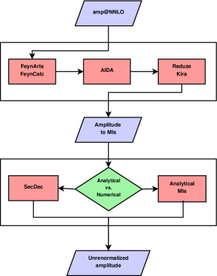
Figure 2: Flowchart of the algorithm

7 Renormalization

QED is a renormalizable theory. As a consequence, UV divergencies arising from divergent loop integrals can be regularized and canceled order-by-order in the coupling expansion.

A diagrammatic approach to the renormalization is the most convenient way to obtain a UV finite amplitude out of the NNLO scattering amplitude; renormalized perturbation theory will be the ideal framework.

In order to renormalize QED, we consider the QED Lagrangian with $N_{f}=1+1$ active flavor, one massive (muon) and one massless (electron) (Bohm:2001yx, ):

$$\mathcal{L}_{0} =-\frac{1}{4}F^{\mu\nu}_{0}F_{0,\mu\nu}+\frac{1}{2\xi_{0}}(\partial_{\mu}A_{0}^{\mu})^{2}$$ (28)

$$+\overline{\psi}_{0}(i\not{p}-m_{0})\psi_{0}+\overline{\chi}_{0}(i\not{p})\chi_{0}$$

$$+e_{0}A^{\mu}_{0}(\overline{\psi}_{0}\gamma_{\mu}\psi_{0}+\overline{\chi}_{0}\gamma_{\mu}\chi_{0}).$$

In this approach, fields, couplings and masses are treated to be bare (denoted with the subscript 0). Bare quantities are connected to the renormalized ones by

$$\begin{gathered}\psi_{0}=Z_{\psi}^{\frac{1}{2}}\psi,\quad\chi_{0}=Z_{\chi}^{\frac{1}{2}}\chi,\\ A^{\mu}_{0}=Z_{A}^{\frac{1}{2}}A^{\mu},\quad\xi_{0}=Z_{\xi}\xi,\\ e_{0}=Z_{e}e,\quad m_{0}=Z_{m}m.\end{gathered}$$ (29)

The bare Lagrangian can be expressed in terms of the renormalized quantites:

$$\mathcal{L}_{0}=\mathcal{L}_{R}+\mathcal{L}_{\text{ct}},$$ (30)

where

$$\mathcal{L}_{R}= -\frac{1}{4}F^{\mu\nu}F_{\mu\nu}+\frac{1}{2\xi}(\partial_{\mu}A^{\mu})^{2}$$ (31)

$$+\overline{\psi}(i\not{p}-m)\psi+\overline{\chi}(i\not{p})\chi$$

$$+eA^{\mu}(\overline{\psi}\gamma_{\mu}\psi+\overline{\chi}\gamma_{\mu}\chi),$$

and

$$\mathcal{L}_{\text{ct}}= -\frac{1}{4}(Z_{A}-1)F^{\mu\nu}F_{\mu\nu}$$ (32)

$$+\frac{1}{2\xi}(Z_{A}Z_{\xi}^{-1}-1)(\partial_{\mu}A^{\mu})^{2}$$

$$+(Z_{\psi}-1)\overline{\psi}(i\not{p})\psi+(Z_{\chi}-1)\overline{\chi}(i\not{p})\chi$$

$$-(Z_{\psi}Z_{m}-1)m\overline{\psi}\psi$$

$$+(Z_{\psi}Z_{A}^{\frac{1}{2}}Z_{e}-1)eA^{\mu}(\overline{\psi}\gamma_{\mu}\psi)$$

$$+(Z_{\chi}Z_{A}^{\frac{1}{2}}Z_{e}-1)eA^{\mu}(\overline{\chi}\gamma_{\mu}\chi).$$

The counterterm Lagrangian $\mathcal{L}_{\text{ct}}$ contains the divergent behaviour arising from the bare quantities.

Ward Identities in QED constrain ratios between the normalizations $Z_{i}$ (Bohm:2001yx, ).

$$\frac{Z_{A}}{Z_{\xi}}=\kappa_{\xi},\quad\frac{Z_{A}^{\frac{1}{2}}}{Z_{\xi}Z_{e}}=\kappa_{e},$$ (33)

where $\kappa_{\xi}$ and $\kappa_{e}$ are arbitrary finite constants. By choosing $\kappa_{i}=1$, the normalizations become

$$Z_{\xi}=Z_{A},\quad Z_{e}=Z_{A}^{-\frac{1}{2}}.$$ (34)

Note that the choice of the renormalization scheme for the photon field $A^{\mu}$ leads automatically to fix the same prescription to the coupling $e$. This is a direct consequence of the Ward Identities (34) in QED .

It is important to stress that Eq. (33) constrains only the divergent part of the normalizations, letting their finite part unconstrained. Hence, two different renormalization prescription for $Z_{e}$ and $Z_{A}$ can be chosen, e.g. $Z_{A}$ in on-shell scheme and $Z_{e}$ in $\overline{\text{MS}}$ scheme. This alternative choice brings the Ward identity to be

$$Z_{e}=Z_{A}^{-\frac{1}{2}}\bigr{|}_{\text{finite}=0},$$ (35)

which yields no contradiction with Eq. (33).

Imposing the Ward identities (33), the counterterms Lagrangian becomes

$$\mathcal{L}_{\text{ct}}= -\frac{1}{4}(Z_{A}-1)F^{\mu\nu}F_{\mu\nu}$$ (36)

$$+(Z_{\psi}-1)\overline{\psi}(i\not{p})\psi+(Z_{\chi}-1)\overline{\chi}(i\not{p})\chi$$

$$-(Z_{\psi}Z_{m}-1)m\overline{\psi}\psi$$

$$+(Z_{\psi}-1)eA^{\mu}(\overline{\psi}\gamma_{\mu}\psi)$$

$$+(Z_{\chi}-1)eA^{\mu}(\overline{\chi}\gamma_{\mu}\chi).$$

Finally, by setting $Z_{i}=1+\delta_{i}$

$$\mathcal{L}_{\text{ct}}= -\frac{1}{4}\delta_{A}F^{\mu\nu}F_{\mu\nu}$$ (37)

$$+\delta_{\psi}\overline{\psi}(i\not{p})\psi+\delta_{\chi}\overline{\chi}(i\not{p})\chi$$

$$-(\delta_{\psi}+\delta_{m}+\delta_{\psi}\delta_{m})m\overline{\psi}\psi$$

$$+\delta_{\psi}eA^{\mu}(\overline{\psi}\gamma_{\mu}\psi)+\delta_{\chi}eA^{\mu}(\overline{\chi}\gamma_{\mu}\chi).$$

The Ward identities have been chosen in such a way that only field and mass renormalization is needed. The coupling constant $e$ is automatically renormalized thanks to the Ward identities.

The counterterm Lagrangian provides additional Feynman rules, which lead to UV finite amplitude. Physical results can only be obtained by choosing a renormalization scheme that fixes the residual unphysical degrees of freedom.

Different renormalization schemes bring changes to the 4-point Green function. The $S-$matrix element $\bra{e\mu}S\ket{e\mu}$ is related to the amputated renormalized Green function $\bra{0}T\{\psi(p_{1})\chi(p_{2})\overline{\psi}(p_{3})\overline{\chi}(p_{4})\}\ket{0}_{amp}=G_{4}$ by

$$\bra{\mu e}S\ket{\mu e} =(\not{p}_{1}-m_{P})\not{p}_{2}\not{p}_{3}(\not{p}_{4}-m_{P})G_{4},$$ (38)

known as Lehmann-Symanzik-Zimmermann (LSZ) reduction formula (Lehmann1955, ; Schwartz:2013pla, ). The Dirac operators $(\not{p}_{i}-m_{P})$ contain the wave-function corrections, and $m_{P}$ is the pole mass of the muon. Different renormalization scheme choices lead to different renormalized masses $m$, introducing a residue at the pole mass $R_{\psi}\neq 1$,

$$\begin{gathered}\lim_{\not{p}\to m_{P}}(\not{p}-m_{P})\frac{i}{\not{p}-m}=R_{\psi}\\ \Downarrow\\ \bra{0}T\{\psi(p)\psi(-p)\}\ket{0}=\frac{iR_{\psi}}{\not{p}-m_{P}}+\text{regular terms}.\end{gathered}$$ (39)

The LSZ reduction formula changes according to the new residue, acquiring new factors (Bohm:2001yx, ):

$$\bra{\mu e}S\ket{\mu e} =(\not{p}_{1}-m_{P})\not{p}_{2}\not{p}_{3}(\not{p}_{4}-m_{P})\frac{G_{4}}{R_{\psi}R_{\chi}}.$$ (40)

Expressing the residue as $R_{i}=1+\delta R_{i}$, the order-by-order structure of the renormalized Green function become manifest

$$\begin{gathered}G_{4}=G_{\text{tree}}+G_{1l}+G_{2l}+\cdot,\\ \delta R_{i}=\delta R_{i,1l}+\delta R_{i,2l}+\cdots,\end{gathered}$$ (41)

which yields to the following structure

$$G_{4} =G_{\text{tree}}$$ (42)

$$+[G_{1l}-(\delta R_{\psi,1l}+\delta R_{\chi,1l})G_{\text{tree}}]$$

$$+[G_{2l}-(\delta R_{\psi,1l}+\delta R_{\chi,1l})G_{1l}$$

$$-(\delta R_{\psi,2l}+\delta R_{\chi,2l})G_{\text{tree}}+\delta R_{\psi,1l}\delta R_{\chi,1l}G_{\text{tree}}].$$

The choice of the on-shell renormalization scheme for the muon mass and fields sets $\delta R_{\psi,i}=0$ identically.

Therefore, the renormalization scheme choice applied in the $\mu e\to\mu e$ scattering is:

• $\overline{\text{MS}}$ scheme for the coupling, the photon and the electron fields

• On-shell scheme for the muon field and mass

The muon field is treated differently due to its non-vanishing mass. Despite of the complications it introduces at integration level, the opportunity to use on-shell scheme for the muon yields simplification at renormalization level.

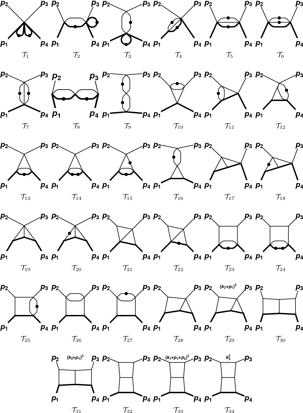
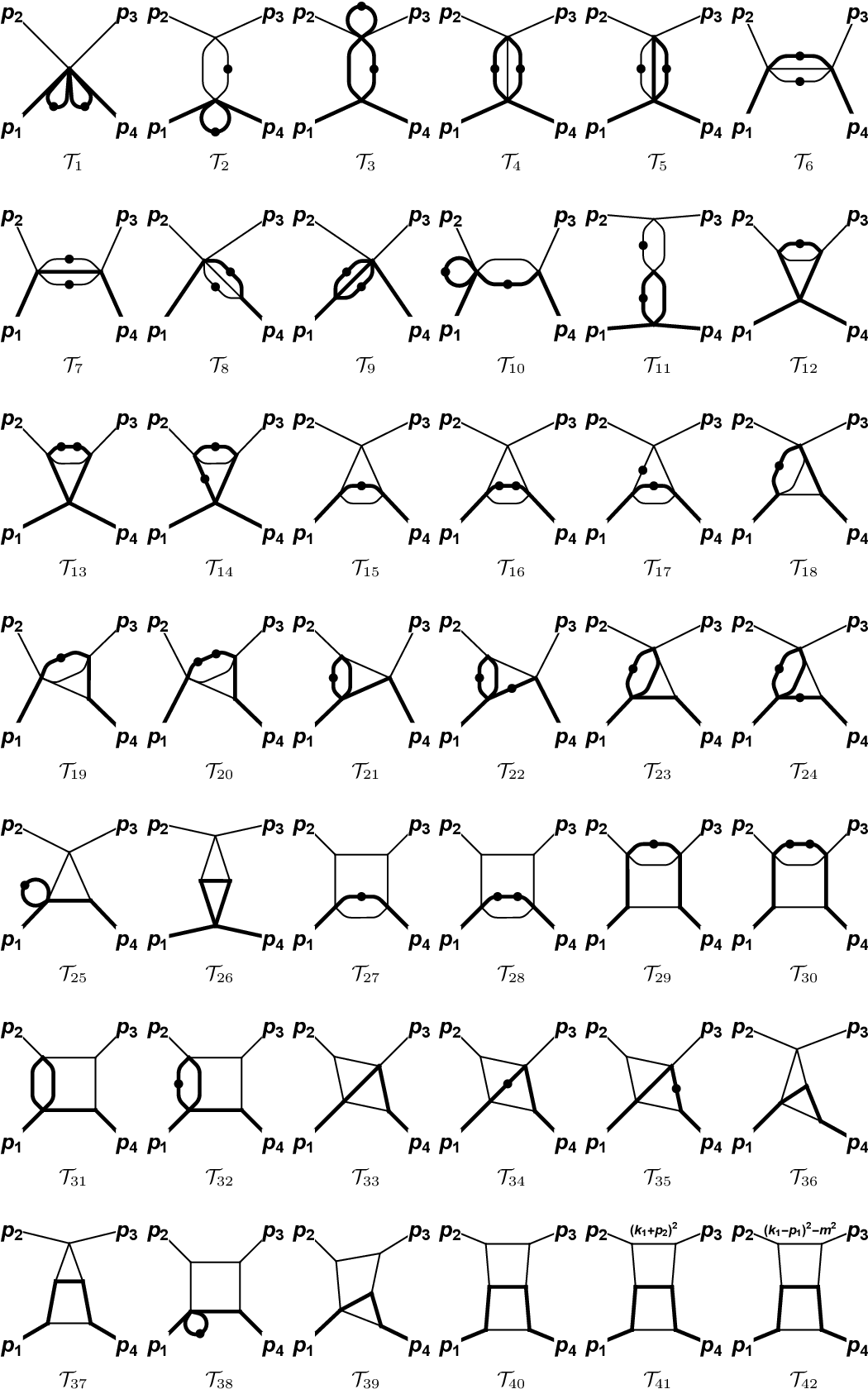
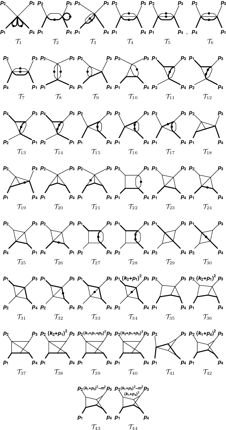
Figure 3: Master Integrals belonging to planar and non-planar topologies for the QED NNLO $\mu e$-scattering amplitude.

8 Summary

There are 69 two-loop Feynman diagrams contributing to the QED NNLO $\mu e$-scattering process (Fig. 1). The complete amplitude gets contributions from $\sim 10^{4}$ Feynman integrals with maximum rank equal to 4.

AID and IBPs reduction with respectively Aida and Kira have decreased significantly the number of integrals (Mastrolia_2017, ; Di_Vita_2018, ), providing $N_{MI}=120$ with max rank equal to 2 (Fig. 3). These MIs are the irreducible set of integrals that one has to evaluate and further reduction of the rank is not possible. The presence of irreducible scalar products, typical of two-loop topology, does not allow a reduction to scalar (rank-0) integrals.

The differential equation method has allowed the analytical evaluation of the planar (Mastrolia_2017, ) and non-planar (Di_Vita_2018, ) sets of MIs. The consistency of the result has been checked by evaluating the MIs with GiNaC and comparing the result with the numerical integration with SecDec, finding agreement between the two approaches.

At the present state of the calculation, the analytical unrenormalized amplitude has been achieved. The renormalization strategy discussed in Section 7 is still in progress. A careful check of the cancellation of the UV divergencies is required in order to obtain a UV finite contribution.

The double-virtual contribution represents the most challenging part of the full $\mu e$-scattering cross section. However, the complete UV/IR finite NNLO amplitude can be achieved only by including all the contributions in Eq. (6). A particular care should be given to the soft and collinear limit due to photon emission from the electron, which in our approximation are treated as massless.

Real-virtual and double-real correction involve 1-loop and tree-level calculations, which can be dealt with the same technology shown in Section 6. For 1-loop amplitudes, additional tools are available on the market e.g. GoSam Cullen2012 or Package-X Patel:2015tea .

9 Acknowledgment

This work has been supported by the Generalitat Valenciana, the Spanish Government and ERDF funds from the EU Commission and the Spanish Centro de Excelencia Severo Ochoa Programme (Grants No. SEJI/2017/019, FPA2017-84445-P and SEV-2014-0398).

References

- (1) T. Blum, A. Denig, I. Logashenko, E. de Rafael, B.L. Roberts, T. Teubner, G. Venanzoni, The muon (g-2) theory value: Present and future (2013), 1311.2198
- (2) C. Carloni Calame, M. Passera, L. Trentadue, G. Venanzoni, Physics Letters B 746, 325â329 (2015)
- (3) G. Abbiendi, C.M.C. Calame, U. Marconi, C. Matteuzzi, G. Montagna, O. Nicrosini, M. Passera, F. Piccinini, R. Tenchini, L. Trentadue et al., The European Physical Journal C 77 (2017)
- (4) M. Alacevich, C.M. Carloni Calame, M. Chiesa, G. Montagna, O. Nicrosini, F. Piccinini, JHEP 02, 155 (2019), 1811.06743
- (5) M. Fael, JHEP 02, 027 (2019), 1808.08233
- (6) M. Fael, M. Passera, Phys. Rev. Lett. 122, 192001 (2019), 1901.03106
- (7) P. Mastrolia, T. Peraro, A. Primo, Journal of High Energy Physics 2016 (2016)
- (8) P. Mastrolia, T. Peraro, A. Primo, W.J. Torres Bobadilla, PoS LL2016, 007 (2016), 1607.05156
- (9) A. Primo, Ph.D. thesis, Padua U. (2017)
- (10) W.J.T. Bobadilla, Ph.D. thesis, Padua U. (2017)
- (11) K.G. Chetyrkin, F.V. Tkachov, Nucl. Phys. B192, 159 (1981)
- (12) Laporta, International Journal of Modern Physics A 15, 5087 (2000)
- (13) A. von Manteuffel, C. Studerus, Reduze 2 - distributed feynman integral reduction (2012), 1201.4330
- (14) P. MaierhÃfer, J. Usovitsch, P. Uwer, Comput. Phys. Commun. 230, 99 (2018), 1705.05610
- (15) G. Barucchi, G. Ponzano, Journal of Mathematical Physics 14, 396 (1973)
- (16) A.V. Kotikov, Phys. Lett. B254, 158 (1991)
- (17) E. Remiddi, Nuovo Cim. A110, 1435 (1997), hep-th/9711188
- (18) T. Gehrmann, E. Remiddi, Nuclear Physics B 580, 485â518 (2000)
- (19) P. Mastrolia, M. Passera, A. Primo, U. Schubert, Journal of High Energy Physics 2017 (2017)
- (20) S. Di Vita, S. Laporta, P. Mastrolia, A. Primo, U. Schubert, Journal of High Energy Physics 2018 (2018)
- (21) G. Heinrich, International Journal of Modern Physics A 23, 1457â1486 (2008)
- (22) G. Ossola, C.G. Papadopoulos, R. Pittau, Nuclear Physics B 763, 147â169 (2007)
- (23) P. Mastrolia, E. Mirabella, T. Peraro, Journal of High Energy Physics 2012 (2012)
- (24) S. Badger, H. Frellesvig, Y. Zhang, Journal of High Energy Physics 2012 (2012)
- (25) F. Tkachov, Physics Letters B 100, 65 (1981)
- (26) G. Passarino, M.J.G. Veltman, Nucl. Phys. B160, 151 (1979)
- (27) A.V. Smirnov, V.A. Smirnov, Journal of High Energy Physics 2006, 001â001 (2006)
- (28) W.L. van Neerven, J.A.M. Vermaseren, Phys. Lett. 137B, 241 (1984)
- (29) P. Mastrolia, E. Mirabella, G. Ossola, T. Peraro, Physics Letters B 718, 173â177 (2012)
- (30) T. Hahn, Computer Physics Communications 140, 418 (2001)
- (31) T. Peraro, JHEP 07, 031 (2019), 1905.08019
- (32) A.G. Grozin, International Journal of Modern Physics A 26, 2807â2854 (2011)
- (33) A.V. Smirnov, A.V. Petukhov, Lett. Math. Phys. 97, 37 (2011), 1004.4199
- (34) J.M. Henn, Physical Review Letters 110 (2013)
- (35) R.N. Lee, Journal of High Energy Physics 2015 (2015)
- (36) M. Argeri, S. Di Vita, P. Mastrolia, E. Mirabella, J. Schlenk, U. Schubert, L. Tancredi, JHEP 03, 082 (2014), 1401.2979
- (37) A. Smirnov, Journal of High Energy Physics 2008, 107â107 (2008)
- (38) A. Georgoudis, K.J. Larsen, Y. Zhang, Computer Physics Communications 221, 203â215 (2017)
- (39) R.N. Lee, Journal of Physics: Conference Series 523, 012059 (2014)
- (40) M. Argeri, P. Mastrolia, International Journal of Modern Physics A 22, 4375â4436 (2007)
- (41) J.M. Henn, Journal of Physics A: Mathematical and Theoretical 48, 153001 (2015)
- (42) W. Magnus, Commun. Pure Appl. Math. 7, 649 (1954)
- (43) S. Blanes, F. Casas, J. Oteo, J. Ros, Physics Reports 470, 151â238 (2009)
- (44) R. Bonciani, A. Ferroglia, T. Gehrmann, D. MaÃtre, C. Studerus, Journal of High Energy Physics 2008, 129â129 (2008)
- (45) R. Bonciani, A. Ferroglia, T. Gehrmann, C. Studerus, Journal of High Energy Physics 2009, 067â067 (2009)
- (46) R. Bonciani, A. Ferroglia, T. Gehrmann, A. von Manteuffel, C. Studerus, Journal of High Energy Physics 2011 (2011)
- (47) S. Di Vita, P. Mastrolia, A. Primo, U. Schubert, Journal of High Energy Physics 2017 (2017)
- (48) R.N. Lee, K.T. Mingulov (2019), 1901.04441
- (49) M. Becchetti, R. Bonciani, V. Casconi, A. Ferroglia, S. Lavacca, A. von Manteuffel, JHEP 08, 071 (2019), 1904.10834
- (50) S. Di Vita, T. Gehrmann, S. Laporta, P. Mastrolia, A. Primo, U. Schubert, JHEP 06, 117 (2019), 1904.10964
- (51) P. Mastrolia, M. Passera, A. Primo, U. Schubert, W.J. Torres Bobadilla, EPJ Web Conf. 179, 01014 (2018)
- (52) S. Borowka, G. Heinrich, S. Jones, M. Kerner, J. Schlenk, T. Zirke, Computer Physics Communications 196, 470â491 (2015)
- (53) T. Hahn, Computer Physics Communications 168, 78â95 (2005)
- (54) M. Bohm, A. Denner, H. Joos, Gauge theories of the strong and electroweak interaction (2001), ISBN 9783519230458, 9783322801623, 9783322801609
- (55) H. Lehmann, K. Symanzik, W. Zimmermann, Il Nuovo Cimento (1955-1965) 1, 205 (1955)
- (56) M.D. Schwartz, Quantum Field Theory and the Standard Model (Cambridge University Press, 2014), ISBN 1107034736, 9781107034730
- (57) G. Cullen, N. Greiner, G. Heinrich, G. Luisoni, P. Mastrolia, G. Ossola, T. Reiter, F. Tramontano, The European Physical Journal C 72, 1889 (2012)
- (58) H.H. Patel, Comput. Phys. Commun. 197, 276 (2015), 1503.01469