Climate bistability of Earth-like exoplanets

Abstract

Before about 500 million years ago, most probably our planet experienced temporary snowball conditions, with continental and sea ices covering a large fraction of its surface. This points to a potential bistability of Earth’s climate, that can have at least two different (statistical) equilibrium states for the same external forcing (i.e., solar radiation). Here we explore the probability of finding bistable climates in earth-like exoplanets, and consider the properties of planetary climates obtained by varying the semi-major orbital axis (thus, received stellar radiation), eccentricity and obliquity, and atmospheric pressure. To this goal, we use the Earth-like planet surface temperature model (ESTM), an extension of 1D Energy Balance Models developed to provide a numerically efficient climate estimator for parameter sensitivity studies and long climatic simulations. After verifying that the ESTM is able to reproduce Earth climate bistability, we identify the range of parameter space where climate bistability is detected. An intriguing result of the present work is that the planetary conditions that support climate bistability are remarkably similar to those required for the sustainance of complex, multicellular life on the planetary surface. The interpretation of this result deserves further investigation, given its relevance for the potential distribution of life in exoplanetary systems.

1 Introduction

Rocky, earth-like exoplanets lying in the habitable zone of their host stars are the most promising targets to search for life outside the Solar System. Because of their small masses and sizes, only a small number of rocky planets have been detected in the surveys carried out with the radial-velocity (Mayor et al., 2011) and transit (Balatha, 2014) methods so far. Nevertheless, planets with Earth-like masses and sizes appear to be intrinsically more frequent than giant planets once the statistics are corrected from the effects of observational bias (Mayor et al., 2011; , 2014; Burke, 2015). Therefore we expect many rocky planets to be discovered in forecoming observational surveys. As statistics increases, the emphasis of the studies will be on the characterization of the planetary properties and the selection of targets with high probability of being habitable for further analysis. Eventually, the selected planets will be the best targets for follow-up observations aimed at looking for the presence of atmospheric compounds of biological origin (Kaltenegger et al., 2015).

In this general scenario, it is important to explore the impact of planetary conditions that may affect the climate and habitability of earth-like exoplanets. Two of such conditions are taken into account in the classic definition of the habitable zone, namely the spectral energy distribution of the host star and the planetary insolation, the latter depending on the orbital semi-major axis and on stellar luminosity. However, planetary climate and habitability are determined by many other physical quantities, such as orbital eccentricity, surface gravity acceleration, atmospheric pressure and composition, obliquity of the rotation axis, rotation rate, and surface distribution of oceans and continents (Pierrehumbert, 2010; Kasting, 2015). In this framework, a particularly interesting issue is the possible existence of multiple stable solutions, for example in terms of multiple stable equilibrium states such as those discussed for Earth and found in numerical simulations of the terrestrial climate (Budiko, 1969; Sellers, 1969; Rose & Marshall, 2009; Ferreira et al., 2011; Linsenmeier et al., 2015). If multiple stable states exist, then the planet can end up in one or the other depending upon the initial conditions. Similarly, external disturbances and the internal turbulent dynamics of the climate system can push the planet out of one state into another stable solution (, 1982). For Earth, this mechanism has been advocated for rationalizing the existence of snowball-like solutions and warm states (Zaliapin & Ghil, 2010). If multiple stable states exist, then observing a planet that is temporarily in a snowball state does not necessarily imply that the planet is not habitable. Indeed, some authors claimed that temporary snowball states are a requisite for the evolution of metazoans with high energy demands (Rose & Marshall, 2009).

In a modelling framework, many of the quantities determining planetary climates are hard to measure with present-day observational facilities and must be treated as free parameters. On top of the difficulty of exploring a multi-parameter space of planetary conditions, one must also face the general issue of how to model planetary climates, for example, in terms of the level of complexity of the selected models. Here, the choice ranges from extremely simplified zero-dimensional Energy Balance Models (EBM), treating the planet as a homogeneous point in cosmic space, see e.g. North et al. (1981); Ghil (1994), to fully-coupled ocean-atmosphere Global Climate Models (GCM), see e.g. primer; Trenberth et al. (xxxx). Between EBMs and GCMs, an entire spectrum of options is available, bearing in mind that the more complex the model is, the larger is the amount of information needed to obtain meaningful results (e.g., the position of the continents and their orography). Given the paucity of information that is currently available on the characteristics of exoplanets, in past years we developed a climate model with an intermediate level of complexity, namely the Earth-like planet Surface Temperature Model (ESTM) discussed by Vladilo et al. (2015) and succintly summarized in Section 3.

In the present work we use the ESTM to investigate what parameter range is associated with the presence of bistability, and compare such range with the conditions for habitability (using the liquid water criterium). This analysis leads to some considerations on the potential links between bistability and habitability for earth-like planets. The presence of bistability is explored by determining the final state (snowball or warm) depending on the initial temperature conditions for a given set of planetary parameters. The impact of the ice-albedo feedback in the context of bistability is specifically addressed.

The systematic exploration of a broad space of planetary parameters, as considered in our study, requires running a very large number of climate simulations. The choice of models with an intermediate level of complexity is thus the most suitable one, since these simple climate models are characterized by a very low usage of CPU. In this work, we explored approximately $10^{5}$ cases using the ESTM. The current work extends and completes a previous study of climate bistability in aquaplanets reported by Kilic et al. (2017) using a simplfied GCM.

The paper in structured as follows. In Section 2 we introduce the general problem of bistability in the context of simplified climate models while in Section 3 we provide a brief description of the ESTM. Section 4 presents the dataset used to build up our collection of climate simulations. In Section 5 we discuss the bistability of Earth climate, as simulated by the ESTM, and in Section 6 we explore the range of parameter values where climate bistability in earth-like exoplanets is potentially present, comparing it with the range where habitability is possible. Finally, Section 7 provides a discussion of the results and some conclusions.

2 Bistability in Energy-Balance Models

Energy Balance Models (EBMs) are simplified thermodynamical descriptions of the surface Earth temperature (Budiko, 1969; Sellers, 1969), and they can be considered as the simplest global climate models (North et al., 1981; Saltzman et al., 2002). The main point of EBMs is that the planetary surface temperature is obtained from a suitably-written form of the first principle of thermodynamics, where the temporal variation of the temperature $T$ is given by the difference between the absorbed solar radiation (for Earth, mostly in the visible part of the spectrum) and the (infrared) radiation emitted by the planet. The absorbed radiation is the fraction of received stellar radiation that is not reflected back to space (that is, the fraction $1-A$ where $0\leq A\leq 1$ is the planetary albedo). At (statistical) equilibrium, the absorbed and emitted radiation at global level are balanced.

EBMs can be zero- or one-dimensional. Simplest versions are zero-dimensional, that is, they describe the globally averaged planet surface temperature, which depends only on time $t$. More refined versions are spatially one-dimensional, that is, they describe the surface temperature as a function of latitude and time. In this version, at each latitude, besides absorbed and emitted radiation, one must include also the divergence of the meridional heat flux, which accounts for the latitudinal heat transport. Often, the heat flux is parameterized by the gradient of temperature, which results in a heat diffusion term in the temperature equation (North et al., 1981; Adams et al., 2003; Wood et al., 2008). In such conditions, most of the uncertainty depends on the proper parameterization of the diffusion coefficient, which in principle can depend on latitude, temperature, and time. In a recent paper (Vladilo et al., 2015), an extended version of the simplest one-dimensional EBM was proposed and tested. The current version of the model, called Earth-like planet Surface Temperature Model (ESTM, see Section 3 for details), uses a more refined definition of the diffusion coefficient mimicking the effects of atmospheric circulation, a latitudinal dependence of the fraction of continental areas, a more precise parameterization of albedo from the ocean and the continents, and a set of one-dimensional vertical column radiative-convective calculations that define the emitted radiation at the top of the atmosphere as a function of surface temperature and atmospheric composition. Simplified prognostic equations for ice-sheet dynamics and for sea ice are also included, as well as a simple prescription for clouds.

In the absence of nonlinear feedbacks, EBMs usually provide a unique (globally stable) equilibrium solution. That is, given the stellar input, the planetary albedo, and the characteristics of the surface and of the atmosphere, the equilibrium temperature where absorbed and emitted radiation balance is uniquely defined.

Classic terrestrial EBMs, however, have long been used to provide a simplified description of the possibility of multiple equilibrium states for the same set of forcing conditions, such as the glacial-interglacial conditions in the last three million years or the emergence of Snowball Earth (or icehouse) states. To clarify this point, we recall that multiple equilibria indicate the possibility of different equilibrium solutions for the same values of external forcing and internal system parameters. The system will then dynamically settle on one specific equilibrium state depending on the initial conditions. External disturbances or the internal natural climate variability (not described in such simple EBMs) could push the planet’s climate from one state to the other.

For multiple equilibria to occur, a nonlinear feedback between temperature and either reflected or emitted radiation (besides the Stefan-Boltzmann law) must be introduced. The simplest and more standard approach is to introduce a feedback between temperature and albedo, based on the presence of ice cover (e.g. Ghil, 1994). Ice albedo is much larger than that of the bare (or vegetated) ground. Thus, for low surface temperature, the ice cover is more extended than for higher temperatures, and the albedo at low T is correspondingly higher. A typical parameterization of this effect is a constant and high albedo below a critical temperature threshold (say a few degrees below the freezing point), when the ice cover is extensive, a constant and low albedo above a upper temperature threshold representing the full melting of ice cover, and a linear dependence between the two threshold. Alternatively, a hyperbolic tangent dependence of albedo on temperature can provide similar results. With such albedo parameterization, for intermediate insolation conditions EBMs may provide two stable equilibria corresponding respectively to fully-glaciated (snowball) condition and to an (almost) ice-free world, and an unstable equilibrium in between these two extremes.

An important point concerns the role of stabilizing (negative) and destabilizing (positive) feedbacks. Negative feedbacks tend to damp the effects of external perturbations, leading to an equilibrium point which can survive external disturbances. A classic example in planetary climates is the homeostatic behavior observed in simple models such as Daisyworld (Watson & Lovelock, 1983; Lenton & Lovelock, 2001; Lenton & van Oijen, 2002; Wood et al., 2008). Here, even a change in the stellar output (such as its increase with time) can be balanced by a change in the surface albedo associated with the dominance of different types of vegetation. By contrast, positive feedbacks tend to amplify the effects of initial perturbations and typically lead to multiple equilibria, as in the examples discussed above, or to runaway situations as in the moist runaway greenhouse effect.

More generally, the stability and bifurcations properties of EBMs and Daisyworld-like models, also including their suitability for the Earth’s climate, have been widely explored, see e.g. Ghil (1976); Rombouts & Ghil (2015). The parameter space for climate stability of Earth-like planets has also been investigated (Alberti et al., 2018). In addition, the evidence of striped patterns in one-dimensional models could be seen as a manifestation of spatial multiple solutions (Adams et al., 2003), closely related to the existence of positive and negative feedbacks changing stability properties (Alberti et al., 2015).

The existence of multiple climate states has been explored also with more detailed Global Climate Models (Rose & Marshall, 2009; Ferreira et al., 2011; Linsenmeier et al., 2015), confirming end extending the results obtained with simpler models. More recently, Kilic et al. (2017) have used an Earth System model of Intermediate Complexity (the “Planet Simulator”, Lunkeit et al., 2011) to study the presence of multiple stable states in aquaplanets, for different values of stellar irradiation and obliquity, finding, also in this case, the potential coexistence of warm and snowball states.

Before closing, a few comments are in order. First, ice-temperature feedback is not the only one that can produce multiple equilibria. Indeed, there are a lot of feedbacks to be considered in building up a climate model that could lead to changes in the stability conditions and to multiple steady state solutions, see e.g. Ghil & Lucarini (2019).

For example, vegetation usually is darker than sandy soils. From this observation, Charney (1975) proposed the possibility of multiple equilibria in arid regions, associated with the presence or absence of vegetation. Extending this approach, (2006) and (2008) showed that multiple equilibria in arid continental regions can also emerge from the fact that the presence of vegetation leads to larger evapotranspiration (and thus more unstable atmospheric stratification) than bare soil. This approach was later extended to a simplified zero-dimensional, columnar model representing a whole arid planet, showing that the presence of vegetation could sustain a hydrological cycle, which would instead disappear for bare ground (Cresto Aleina et al., 2013). Finally, also the albedo effect of cloud cover has been shown to be able to increase the number of coexisting multiple equilibria.

A second point concerns the possibility of oscillating or chaotic solutions, something well known in low-order dynamical systems but not very common in EBMs. Early attempts to obtain self-sustained oscillatory solutions in EBMs considered coupling ice sheets, atmosphere and ocean (Kallen & Crafoord, 1979) or an EBM coupled with ice-sheet dynamics and the slow isostatic response of the viscous flow in the upper mantle (Ghil & Le Treut, 1981). Also for limit cycles (self-sustained oscillations) and chaotic solutions, it is possible to have multiple solutions for the same external forcing levels, as discussed by Lorenz (1990). In general, however, obtaining self-sustained oscillations requires at least two coupled dynamical equations, and it is a behavior that is not expected in the simplest EBM or ESTM approaches.

3 THE ESTM MODEL

The model adopted here is the Earth-like planet surface temperature model (ESTM) described in detail by Vladilo et al. (2015). The core of the model is a one-dimensional Energy Balance Model (EBM) fed by multi-parameter physical quantities and written for an elliptical orbit and taking into account the planet axial tilt (thus, incorporating the seasonality of the stellar radiation intercepted by the planet). The dynamical variable is the planet surface temperature $T(\phi,t)$, that is a function of latitude $\phi$ and time $t$. All relevant quantities are thus zonally averaged. As an improvement over classic EBMs, the vertical transport in ESTM is described using single-column atmospheric calculations, while meridional transport is parameterized based on the results of full 3D climate model simulations.

By assuming that the heating and cooling rates and the meridional heat transport are balanced at each latitude, one obtains an energy balance equation that is used to calculate $T(\phi,t)$. The most common form of EBM equation (North et al., 1981; Williams & Kasting, 1997; Spiegel et al., 2008; Pierrehumbert, 2010; Gilmore, 2014)

$$C\frac{\partial T}{\partial t}=S(1-A)-I+\frac{\partial}{\partial x}\left[D(1-x^{2})\frac{\partial T}{\partial x}\right]$$ (1)

where $x=\sin\phi$ and all terms are normalized per unit area. The term on the left hand side of this equation represents the zonal heat storage and describes the temporal evolution of each zone; $C$ is the zonal heat capacity per unit area (North et al. 1981). The first term on the right hand side representes the absorbed stellar radiation, $S$ is the incoming stellar radiation in $W/m^{2}$ and $A$ is the planetary albedo at the top of the atmosphere, function of both temperature and latitude.

In the ESTM, the dependence of albedo $A$ on temperature is not directly imposed, but it is naturally parameterized by the latitudinal dependence of the ice cover on temperature. The total albedo at each latitude is then given by the weighted average between the albedo of the land or ocean and the (larger) albedo of the (continental or sea) ice. This approach provides similar results as a direct parameterization of albedo on temperature, but it has the advantage of introducing a more physically-based description of the processes at work. Thus, as it will be shown below, also for one-dimensional ESTM there is the possibility of multiple equilibria whose existence relies on a temperature-albedo feedback mechanism.

The second term on the right hand side of eq. (1), $I$, represents the thermal radiation emitted by each zone, also called Outgoing Longwave Radiation (OLR). While in simple EBMs this is given by the Stefan-Boltzmann law corrected for greenhouse effects, here the OLR is obtained from detailed vertical column calculations taking into account radiative-convective processes. The third term represents the amount of heat per unit time and unit area leaving each zone along the meridional direction (North et al., 1981). It is called the diffusion term because the coefficient $D$ is defined on the basis of the analogy with heat diffusion, i.e.

$$\Phi\equiv-D\frac{\partial T}{\partial\phi}$$ (2)

where $2\pi R^{2}\Phi\cos\phi$ is the net rate of energy transport across a circle of constant latitude and $R$ is the planet radius (see Pierrehumbert, 2010).

Thanks to a physically-based parameterization, the ESTM features a dependence on surface pressure, $p$, gravitational acceleration, $g$, planet radius, $R$, rotation rate, $\Omega$, surface albedo, $a_{s}$, stellar zenith distance, $Z$, atmospheric chemical composition, and mean radiative properties of the clouds. In a typical simulation, the ESTM generates the temporal dynamics of the surface temperature $T(\phi;t)$ starting from a given initial conditions $T_{0}(\phi)$. Full details on the ESTM are given in Vladilo et al. (2015).

In the ESTM different temperature-based habitability criteria can be adopted. In this work, habitability is defined based on a liquid water criterion for the presence of complex life (Silva et al., 2016): that is, potentially habitable conditions correspond to a temperature range between the freezing point of water (for a given atmospheric pressure) and an upper limit $T\approx 50$ C needed for the persistence of active metabolism and reproduction of multicellular poikilotherms (organisms whose body temperature and functioning of all vital processes is directly affected by the ambient temperature). We thus adopt a habitability index for complex life, $h_{050}$, representing the mean orbital fraction of planetary surface that satisfies the above temperature limits, see Silva et al. (2016) for further details.

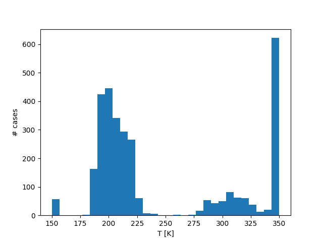
Figure 1: Histogram of the final annual global average temperatures for all of our 86422 valid runs (including those that did not converge, but ended up in a runaway greenhouse situation or an automatic snowball one). Note that, clearly, the histogram is obtained using the number of cases not that of quadruplets.

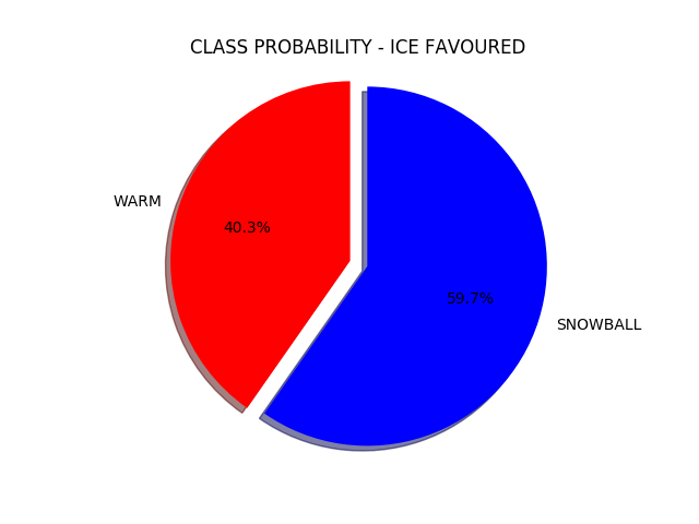
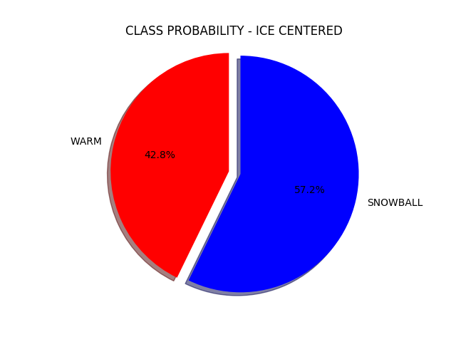
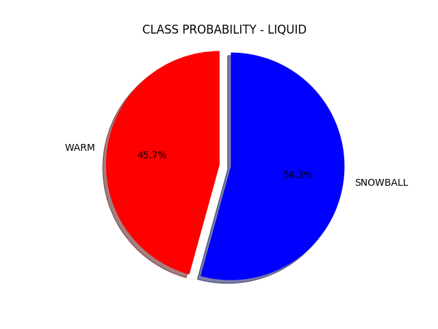
Figure 2: Probability of having WARM or SNOWBALL cases, for the three different probability support defined in Section 4. We integrated over the whole parameter set and did not distinguish stable from bistable cases.

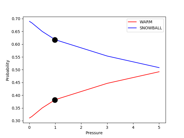
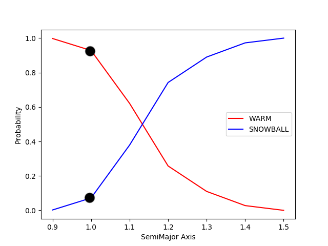
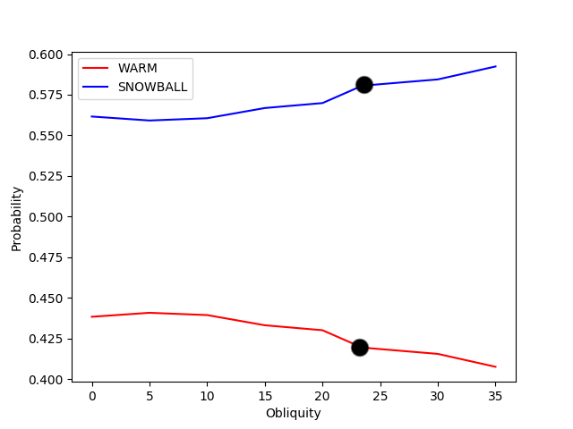
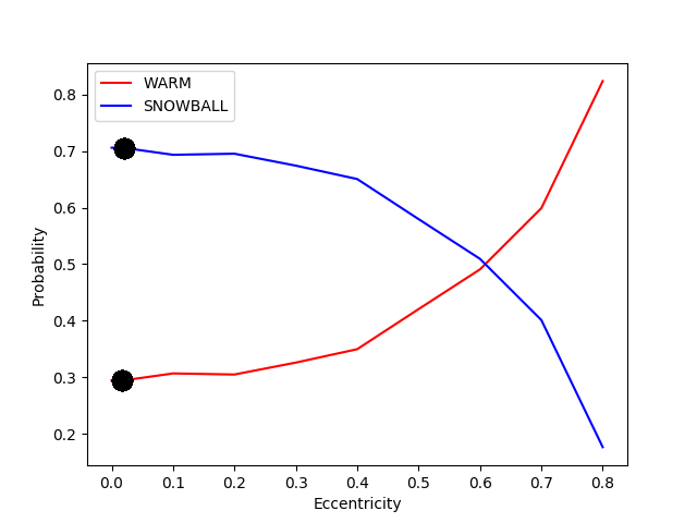
Figure 3: Probability of having a WARM and SNOWBALL cases, as a function of our four parameters separately. For each parameter, we calculated the probability using Equation 6, and estending the summations in Equation 5 to all the indexes of the other four parameters. Upper-left panel: probability as a function of pressure; Upper-right panel: probability as a function of semi-major axis; lower-left panel: probability as a function of obliquity; lower-right panel: probability as a function of eccentricity. In red the probability to end up in the WARM class, in blue that to end up in the SNOWBALL one. Here we show results for the IceCentered probability support. Black dots show the position of Earth in each plot.

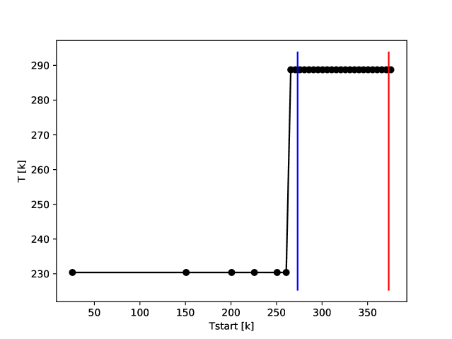
Figure 4: Annual global average temperature in the stationary state, as a function of initial temperature for the Earth case, quadruplet with {pressure, semi-major axis, obliquity, eccentricity}={1.0, 1.0, 23.4393,0.01671022}. The blue and red vertical lines mark the freezing and boiling temperature.

Table 1: Parameters used for our ESTM model runs. Column 1: parameter; Column 2: values. Pressures in bar; Semi-Major axis in Astronomical Units; Obliquities in degrees; for Initial Iemperatures we give the index $i_{T}$ of $T_{\rm init}=T_{\rm freeze}+i_{T}\cdot dT$, see text for mode details. Column 3: indexes used in Equation 5

Parameters	Value	index
Pressures	0.01, 0.1, 0.5, 1.0, 3.0, 5.0	$i_{p}$
Semi-Major Axis	0.9, 1.0, 1.1, 1.2, 1.3, 1.4, 1.5	$i_{r}$
Obliquities	0., 5., 10., 15., 20., 23.4393, 30., 35.,	$i_{o}$
Eccentricities	0.0, 0.01671022, 0.1, 0.2, 0.3, 0.4, 0.5, 0.6, 0.7, 0.8	$i_{e}$
Initial temperatures	-50, -25, -15, -10, -5, -3, -2, -1,0,1,2,3,4,5,6,7,8,9,10,11,12,13,14,15,16,17,18,19,20	$i_{T}$

4 The Dataset

We run the ESTM varying four parameters, namely pressure, orbital eccentricity, inclination of the rotation axis and semi-major axis (SMA) of the orbit, for a total of $N_{\rm param}*N_{T_{\rm init}}=97440$ cases. $N_{\rm param}=3360$ is the number of independent simulations, each of which is run using $N_{T_{\rm init}}=29$ different initial temperatures.

We set the initial temperatures using:

$$T_{\rm init}=T_{\rm freeze}+i_{T}*dT$$ (3)

where $T_{\rm freeze}$ is the pressure-dependent freezing point of water, and

$$dT=(T_{\rm boil}-T_{\rm freeze})/20$$ (4)

here $T_{\rm boil}$ is the pressure-dependent water boiling temperature and $i_{T}=1,...,20$. Thus we have 20 different initial temperatures in the pressure-dependent liquid water temperature ranges. We added 9 more values at or below the freezing temperature of water, since we determined that the onset of bistability in our model can happen below such a temperature (see Section 5). In Table 1 we list the parameter values used.

All other model parameters, and in particular: radius of the planet, mass of the planet, chemical composition of the atmosphere, rotation period of the planet, type of star of the system, partial methane (CH₄) and carbon dioxide (CO₂) pressures, are set to Earth values. We used a fixed constant fractional ocean coverage of 70%.

Given a set of parameters, usually the ESTM converges to an annual oscillation, where the surface temperatures in each latitudinal band and at each given position in the orbit have the same value for the different years. We verified this behavior by asking that the global annual average temperature (averaged over the latitudes at a given position in the orbit) does not change by more than 0.01 K from one year to the next. After convergence has been reached, we record a number of model outputs; we focus our analyses on the global annual surface temperature $T_{\rm fin}$ and the fractional ice coverage $f_{\rm ice}$.

However, the model can exit for reasons different from convergence. If more than 50% of the planet surface has a temperature above the water boiling point, we consider such a planet to have high probability of entering a runaway greenhouse state and stop the numerical simulation. In this case we assign a conventional final temperature of 350K. When the maximum temperature of the planet, considering all the latitudinal bands and 48 position on the orbit, is lower than 200 K, we also interrupt the run and consider the planet prone to reach a permanent snowball state. In this case, the conventional final temperature is set to 150 K; we called these cases “automatic snowballs” and we implemented a forced exit in these cases, in order to speed-up the calculations.

Moreover, there are a number of cases in which a run can end traumatically. This happens: (i) if the total (dry plus water vapour) pressure exceeds 10 bar; (ii) if the integration step becomes smaller than 1 hour. Both cases correspond to situations where the hypotheses that our model is based upon are not valid any more. Usually, these traumatic exits happen for extreme values of some parameters, for instance, for very high orbital eccentricities and/or small semi-major axis. These runs must be discarded. Our dataset includes 289 quadruplets of parameters leading to the kind of exits describe above.

In a very limited number of cases, it may also happen that the run does not converge after a given number of orbits. We set this number to 100. The reason is that our continental ice model is based on the annual average temperature in each latitudinal band (owing to the slow response time of ice sheets) and in some situation the ice/albedo feedback may cause the albedo to have a non-periodic, non-converging behavior. This happened for 20 quadruplets, which we also discarded.

At high pressures, it may happen that the initial temperature corresponding to $i_{T}=-50$ in Equation 3 would be negative (in Kelvin). This happened for 1125 quadruplets and we of course discarded such initial conditions.

Finally, for 61 quadruplets, some of our runs with different initial temperatures ended with a traumatic exit. We kept these cases and considered only the runs that converged.

All together, we have a total of 3051 complete or partial quadruplets of parameters, for a total of 86422 valid runs.

The final average temperatures for all the considered quadruplets starting from the different temperatures used for initial conditions, for a total of 86422 valid runs including those that did not converge but ended up in a runaway greenhouse situation or an automatic snowball one, are shown in figure 1. The figure shows that there are two different classes of final average temperatures, that can be neatly separated using a temperature threshold of $T_{\rm thresh}=250$K. We thus define two classes of solutions and call WARM those solutions having a temperature higher than $T_{\rm thres}$, and SNOWBALL the other ones. Our criterion for a run to be classified as SNOWBALL is that its final global annual average temperature is lower than the water freezing temperature $T_{\rm freeze}$, and the surface fraction covered by ice must is grater than 90%, otherwise its class is WARM. This is for taking into account cases where an equatorial belt with temperatures larger than the $T_{\rm freeze}$ coexist with large polar ice caps, so that the global annual average temperature can be lower than $T_{\rm freeze}$. We note that this never happens when the final temperature is lower than 250 K.

Having defined the two classes of solutions, we need a definition for the probability to end up in one of those classes. Our four-dimensional parameter space defined by pressure, semi-major axis, obliquity, and eccentricity is not evenly sampled by our parameter set; moreover, theoretically pressures, semi-major axes and initial temperatures can take a range of values much larger than those we used.

For this reason, we define a volume element of the (five dimensional) parameter and initial conditions space as follows:

$$dV[\vec{i},i_{T}]=dP(i_{p})\cdot dR(i_{r})\cdot dO(i_{o})\cdot dE(i_{e})\cdot dT(i_{T})$$ (5)

where $\vec{i}={i_{p},i_{r},i_{o},i_{e}}$ is the position of a quadruplet in the parameter space, and the differentials are the difference on each of the five axis between two subsequent values of any parameters, e.g. $dP(i_{p})=P(i_{p}+1)-P(i_{p})$. The integer indices $i_{p},i_{r},i_{o},i_{e},i_{T}$ refer to the corresponding values in Table 1. We extend the definition for the last point of each set by taking the interval equal to the point before the last one, e.g. $dP(i_{p{\rm max}})=dP(i_{p{\rm max}}-1)$. Using Equation 5 the probability of SNOWBALL of one quadruplet becomes

$$P_{\rm snow}=\frac{\sum_{i_{T}=1}^{29}dV[\vec{i},i_{T}]_{\rm snow}}{\sum_{i_{T}=1}^{29}dV[\vec{i},i_{T}]}$$ (6)

where $dV[\vec{i},i_{T}]_{\rm snow}$ are the volume elements corresponding to cases of the quadruplet $\vec{i}$ that belong to the class SNOWBALL while $dV[\vec{i},i_{T}]$ are all the volume elements of valid cases of $q$. Of course, $P_{\rm warm}=1-P_{\rm snow}$. Note that the probability defined in Equation 6 is automatically normalized to one, takes into account the uneven sampling of the parameter space, and the fact that for some quadruplet some of the runs in the initial temperature set could not have converged.

Obviously, Equation 6 can be generalized, e.g., to estimate the overall probability to have a SNOWBALL or a WARM case, just by summing over all the runs (dropping $q$ in the equation), or by defining marginal probabilities and integrating on some of the parameters.

The estimated probability $P_{\rm snow}$, as we defined it, clearly depends on its support. The semi-major axis, the eccentricities and the obliquities are evenly spanned, with the exception of the cases $23.4393$ for the obliquity, $0.0167$ for the eccentricity, which we included to have Earth conditions in the dataset. ESTM does not allow us to study obliquities larger than 40 degrees, and we verified that already at 40 degree the model shows unexpected behaviour. The same holds for pressures: values lower than about 0.01 bar and higher than 10 bar are outside the range of validity of our model (see Vladilo15). Semi-major axes smaller than 0.9 AU or larger than 1.5 AU can be studied with ESTM, but when the central star is Sun-like, they are uninteresting as they always end respectively in snowball or runaway greenhouse situations. For these reasons, the parameter space is relatively well defined.

Instead, the initial temperatures are critical. While it is not reasonable to start with very hot or very cold cases, that would behave, in our ESTM model, as very small or very large distances from the star, the specific definition of the probabilty support in the intermediate initial temperature range do change the estimate of the fraction of cases ending up in one or the other state. . For this reason, in the following we define three different supports, where we keep always the whole set of pressures, semi-major axes, obliquities and eccentricities but use:

• The whole initial temperature range of our dataset. Since we span a larger interval of initial temperatures reaching values lower than the freezing temperature, we call this support IceFavoured

• Temperatures from $i_{T}=-15$ to $i_{T}=20$, where $i_{T}$ is the index we used in Equation 3. We call this support IceCentered

• Only initial temperatures above the freezing point of water, from $i_{T}=0$ to $i_{T}=20$. This support is called Liquid.

In Figure 2 we show the probability of having WARM or SNOWBALL cases, for the three different probability supports defined above, integrating over the whole parameter set and initial conditions. The overall trend is as expected, with the Liquid probability support giving more WARM cases than the IceFavoured one, and the IceCentered support taking an intermediate value. However, the fact that the figures are not dramatically different suggests that our choice of the parameter space volume is reasonable; for example, including more large semi-major axis values would have simply increased the number of SNOWBALL situations.

To further explore these states, Figure 3 shows the marginal probabilities of ending in a SNOWBALL or a WARM state depending on the value of each of the four parameters considered, integrating over all values of the remaining three parameters and initial conditions, when the IceCentered support is used. Similar results are obtained for the Liquid support, in that case with a larger fraction of WARM states.

From these overall results, several observations can be drawn:

• As expected, the probability of SNOWBALL increases for larger values of the SMA, independent of the other parameters. The SNOWBALL state becomes the only possible state for SMA about 1.5 AU.

• The probability of WARM states grows with the pressure, integrating over all other parameters and initial conditions.

• The marginal probabilities of WARM and SNOWBALL states remains approximately the same for eccentricity lower than about 0.3, then the probability of WARM states grows rapidly at larger values of the eccentricity. In some of such cases, the planet goes to a runaway greenhouse state.

• Obliquity does not have a strong influence on the probabilities of WARM and SNOWBALL states, with a rather small trend towards more SNOWBALL states for larger obliquities.

• In general, the initial temperature leading to SNOWBALL in the bistable cases is less than or equal to the freezing point of water (figure not shown). Higher initial temperatures lead to the WARM state.

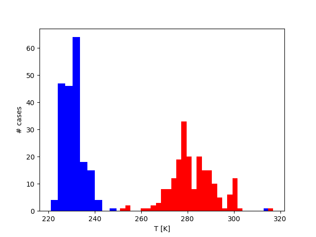
Figure 5: Histogram of the final annual global average temperatures for the bistable quadruplets, in blue the histogram for the lower final annual global average temperatures, in red the istogram for the higher ones. Note that the histograms are made using the number of cases not that of quadruplet

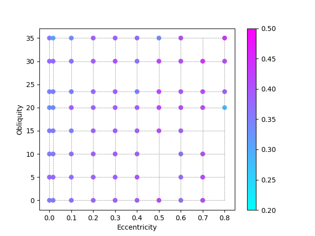
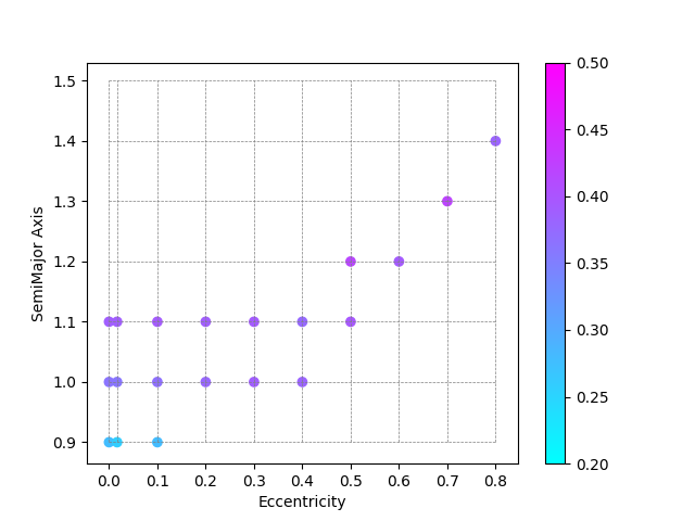
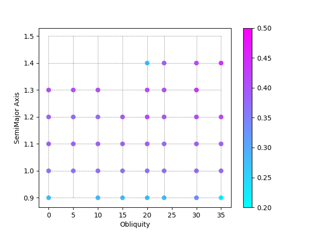
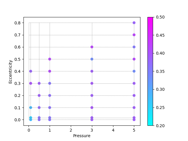
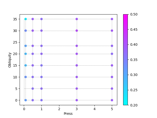
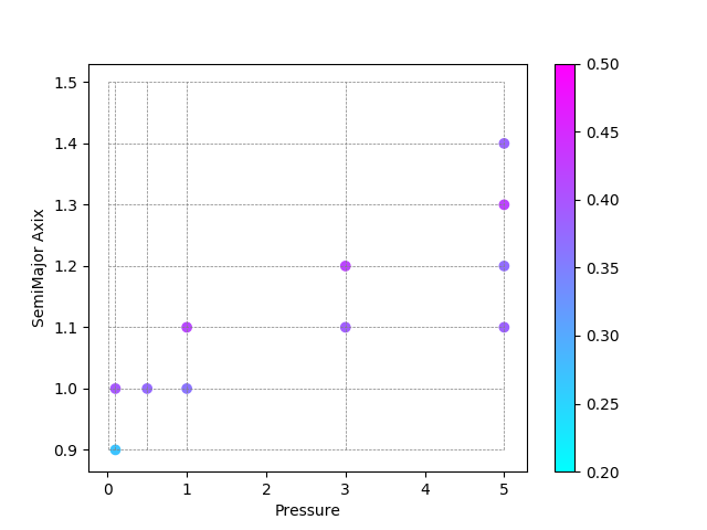
Figure 6: 2D marginal probabilities from the 4D parameter space for the probability support IceCentered. In the panels we show the probability of having a SNOWBALL case as a function of all the couples of parameters, color coded as shown in sidebars. The probability is calculated using Equation 6, where the summation in Equation 5 runs on the indexes that refers to the parameters not in the plotted couple. The grid shows the parameters we used in the dataset. We only plot dots where bistability happens; no dot at an intersection means that for that couple of parameter values there are no bistable cases. Upper left, upper right, middle left, middle right, lower left, lower right panes respectively to the couple of parameters:eccentricity & obliquity, eccentricity &semi-major axis, obliquity & semi-major axis, pressure &eccentricity, pressure & obliquity, pressure & semi-major axis.

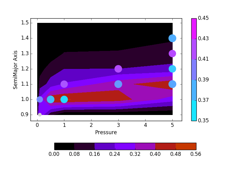
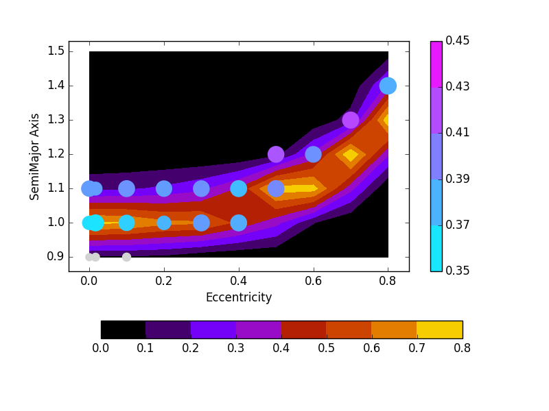
Figure 7: 2D marginal probability from the 4D parameter space for the probability support IceCentered, comparing bistability and habitability. The points indicate bistable solutions and the color coding of the points indicates the probability of having a SNOWBALL case, color coded as in the vertical bar. Small grey points indicate bistable cases with a SNOWBALL probability lesser than 0.35; they are rare and usually get values of about 20-25%. The color map indicates the habitability parameter (between zero and one) for complex life, $h_{050}$, as color coded in the horizontal bar and obtained using the definition from Silva et al. (2016). Top panel: Pressure vs. Semi-Major Axis. Bottom panel: Eccentricity vs. Semi-Major Axis.

5 Bistability of the Earth case in ESTM

Using the ESTM, we first investigated the possible presence of multiple equilibrium states for a set of conditions which are typical of the Earth. These are summarized by the following quadruplet: Pressure $=1.0$ bar, Semi-Major Axis $=1.0$ AU, Obliquity $=23.4393^{\circ}$, and Eccentricity $=0.01671022$. Thus, for the same value of the solar constant, we chose several different values of the initial temperature (as detailed in Table 1 ) and we calculated the annual mean global temperature of the Earth reached in the stationary state after the initial transient. The results are shown in Figure 4: two main climatic regimes are identified, representative of the SNOWBALL and WARM regimes, characterized by a temperature range of 25.90 K - 260.66 K and 265.66 K - 370.55 K, respectively. Thus, the transition between one state and the other occurs for an initial temperature value between 260 and 265 K. Therefore, for the present-day value of the solar constant, in a given range of initial temperatures the global mean temperature converges to 289.42 K, corresponding to the warm case, while for another range of initial temperatures the solution converges to 231.79 K, corresponding to the fully ice-covered case. We can summarize these findings as follows:

• The current astronomical conditions of the Earth support two possible steady climate states, one corresponding to the present climate and the other characterized by much lower temperatures. Depending on the initial temperature, the system is attracted to one of these states (see also Alberti et al. (2015) and Rombouts & Ghil (2015)) .

• Under current initial temperature conditions (in the range of liquid water), the transition to a snowball state is unlikely, unless a change in insolation or in other elements of the Earth’s radiation budget, such as one caused by strongly reduced levels of CO₂ or other Green-House gases (GHG)s, or by a strong increase in stratospheric aerosols, occurs.

An important point is that we verified that the bistability observed here is driven by the ice-albedo feedback. In fact, we run another “Earth” quadruplet artificially removing the ice-albedo feedback: in this case, no bistability develops. Furthermore, both for a smooth transition between bare surface and ice cover (as adopted in the standard ESTM) and for “istantaneus” ice - no ice transition (that is, ice appears as soon as the temperature drops below the freezing point of water), we recover the bistability. Noticeably, the transition between the two states happens at the same limit temperature. This suggests that the behaviour of the climate in ESTM does not depend on the detailed parametrization of ice but only on its presence and response to temperature.

These results show that the ESTM provides results on Earth climate bistability which are consistent with those found using simpler Energy Balance Models. For example, also in studies using EBMs, the likelihood to enter a snowball-Earth climate seems to be quite small (e.g. Zaliapin & Ghil, 2010).

6 Climate bistability in earth-like exoplanets and its links with habitability

To proceed with a full exploration of the climate bistability in earth-like exoplanets, we first need to properly define: (i) what we mean with stability and bistability; (ii) how we define and compute probabilities.

We define a stable solution, one for which all the initial temperatures for a given quadruplet of parameter values produce the same final annual global average temperature. In dynamical systems terms, this is a globally stable solution. A bistable solution instead occurs when two of such final temperatures are produced for the same quadruplet, depending on the initial conditions. Multistable solutions are characterized by a larger number of stable states, but these solutions have not been found in our exploration of the ESTM.

Note that we did detect quadruplets showing more than two temperatures, as described in Section 4. However, we verified that in none of the such quadruplets, we had a situation with convergence to more than two final stable states with different temperatures. Rather, is such cases oscillating behaviours and/or no convergence after 100 orbits was observed. All those cases are peculiar and genuine tri-stability never occured with ESTM, at least within the parameter space which we explored.

The following question is how many quadruplets are associated with two possible final states, reached for different values of the initial conditions. These are the true bistable cases. We identified such bistable cases by searching for the quadruplets where the final average temperatures display significant differences depending on the initial temperature. This search provided 179 quadruplets that are associated with bistable solutions. Figure 5 shows the histogram of the higher (red) and lower (blue) final temperature when we had bistability (compare it with Figure 1). Note, also, that when a quadruplet shows bistability, almost always the runs ending in the lower temperature state are SNOWBALL and the others are WARM. All the other quadruplets lead to a single final stable solution.

For the bistable quadruplets, Figure 6 shows 2D projections (i.e., marginal probabilities) of the 4D parameter space for the probability support IceCentered. In the different panels we show the marginal probability of having a SNOWBALL case as a function of a given parameter couple, color coded as shown in sidebars and integrated over the other two parameters. Some of the quadruplets have almost equal probability of ending up in a WARM or SNOWBALL state depending on initial temperature.

From this figure, a few comments can be drawn:

• Bistable cases are found for almost all parameter values of pressure, eccentricity and obliquity.

• Pressure and obliquity have rather limited effect on the existence of bistability, that is, one can find bistable solutions for any value of these parameters;

• bistability is confined to a well defined range for the semi-major axis, a behavior which is especially visible in the SMA-pressure and SMA-eccentricity plots.

Clearly, the quantitative aspects of these results depend on the support chosen for the initial temperatures: using only initial temperatures above the freezing point drastically reduces the probability of ending up in a SNOWBALL state and thus the presence of bistability.

A final important point concerns the relationships between bistability and habitability. From Figure 6, it is clear that bistability is confined to a rather narrow range of orbital semi-major axis values, which varies with eccentricity and pressure. Figure 7 compares the range where bistability was observed with the range where the conditions for the presence of complex life, as defined by Silva et al. (2016), are fulfilled. Top panel shows the connection among pressure, semi-major axis, bistability and habitability. Bottom panel show the same, but using eccentricity.

This figure reveals the intriguing result of a close similarity between the ranges where “complex life habitability” and bistability are found: if a planetary climate fulfills the habitability criterion, then the same climate is potentially bistable. The interpretation of this result in terms of thermal dependence of biological processes is beyond the purpose of the present work. Here we note that the conditions of bistability allow for the simultaneous presence of two fundamental feedbacks of the climate systems, namely the ice-albedo feedback and the temperature-water vapour feedback. Since these two feedbacks have opposite responses to variations of insolation, they may help to provide a long-term persistence of liquid-water habitability conditions.

We also note that the vast majority of bistable and habitable cases have similar probabilities of being snowballs or warm.

In Figure 7, we note that at high eccentricities and relatively low values of the semi-major axis, high habitability does not correspond to bistable cases. This is because, at these extreme eccentricities, the planet can be warmed-up very fast at the pericenter; this melts the initial ices. Then, only if the semi-major axis is large enough, ice can re-form and bring the system again to a SNOWBALL case. This behaviour does depend on the details of the ice treatment that in ESTM is, of course, simplified. In these extreme cases, a study with intermediate-complexity models, e.g. PLASIM (Fraedrich, 2012), would be needed.

7 Discussion and Conclusions

The main results of this work are that

• Climate bistability is relatively common but not widespread in planetary climates. For 179 quadruplets over the total of 3051 valid quadruplets explored in our study, bistability was clearly detected. In no case we observed more than two stable states. For all other quadruplets for which converge occurred, the climate ended in either a WARM or a SNOWBALL state.

• Bistability generally includes a WARM state, similar to the current state of our planet, and a SNOWBALL state, presumably analogous to what happened to Earth in its past history.

• Although not widespread, the parameter range where bistability occurs is quite similar to the range where habitability conditions for complex life are present.

These results have a few implications that are worth discussing. First, the model runs suggest that climate bistability can occurr in earth-like exoplanets under a variety of parameter values, as suggested by Kilic et al. (2017) for aquaplanets. Thus, for the same external control parameters (stellar luminosity, orbital characteristics and gross atmospheric properties), the planet can either be in a WARM state or in SNOWBALL conditions. Clearly, the two states lead to very different environmental and planetary conditions.

We verified that in our model the transition to a snowball state usually happens when the initial temperature is below the freezing point of water. In our ARTECS database, we always used a “cold start” initial condition, but here “cold” means “sligthy above the freezing point”. The current work thus suggests that the database initial conditions are appropriate to maximize the WARM cases. In an ongoing work, we will use ARTECS to better characterize the habitability of earth-like exoplanets, keeping in mind that we are using the most favourable temperature initial condition for complex life.

In our simple modelling approach, the planet can end up in either a SNOWBALL or WARM state depending on initial conditions, without any possibility to alternate between the two states (as happened to Earth). In reality, a variety of mechanisms can trigger the transition from a WARM to a SNOWBALL state or viceversa. One essential mechanism is the reduction (for triggering the SNOWBALL) or accumulation (to end the SNOWBALL period) of carbon dioxide in the atmosphere, owing to volcanic outgassing, the geological carbon cycle, extreme weathering or biospheric activities (see e.g. Broecker, 2018). In our model, the carbon dioxide content of the atmosphere is fixed and no transitions can be observed. Future work will consider an imposed variable atmospheric carbon dioxide concentration as well as the inclusion of a simplified carbon cycle in the ESTM.

Finally, one of the most intriguing results of this work is the indication that the range of values where climate bistability was found is very similar to the range where the planet can host complex life. This certainly occurred for Earth, and one can wonder whether there may be deeper links between the presence and evolution of complex life and the possibility of entering and exiting a SNOWBALL state (Rose & Marshall, 2009), or even between the presence of climate bistability and plate tectonics activity through its effects on the geological cycle of carbon dioxide. Clearly, these issues cannot be addressed with the simplified approach adopted here, but our results point to the need for further exploring these aspects. Finally, we note that, at least for the Earth case, in the model the transition occurs at an annual global average temperature of -13^∘ C. This means that strong changes in the climate forcings are required to initiate a snowball.

Appendix A ARTECS

Our ARTECS (Archive of terrestrial-type climate simulations) database is aimed at parameter space exploration of exo-climes using ESTM. Currently, we investigated changes in pressure, semi-major axis, eccentricity, obliquity, planet geography and CO₂ partial pressure. Parameter values can be found in Table 2. All runs have “cold start” initial conditions, thus a constant temperature $T=275$K at all latitudes.

ARTECS is public and can be reached at the site http://wwwuser.oats.inaf.it/exobio/climates/. The user can make queries to the archive using parameter values, results (e.g. surface temperature, habitability, etc.), or both.

Results of queries can be downloaded in form of text tables, if only a summary is needed. Detailes FITS maps of surface temperatures vs. time (i.e., orbital position) and latitude can also be downloaded.

ARTECS currently contains 20284 cases: we put on the archive only “converged” runs, thus automatic snowballs, runaway greenhouse cases and failed integrations are not reported. We plan to extend the archive to also varying planet radius, rotation period and surface gravity. To allow scriptin access to ARTECS, a Python3 interface to access ARTECS (py_artecs) have been prepared by our group. The interface with instructions to download, install and use it can be recovered from the ARTECS website or through git at the url https://www.ict.inaf.it/gitlab/michele.maris/py_artecs.git

Table 2: Parameters varied in the ARTECS archive. Pressures in bar; Semi-Major axis in AU; Obliquities in degrees, CO₂ partial pressure in Earth units (we used 380 ppm). Ocean fraction only applies to the first geography.

Parameters	Value
Pressures	0.01, 0.1, 0.5, 1.0, 3.0, 5.0
Semi-Major Axis	0.9, 1.0, 1.1, 1.2, 1.3, 1.4, 1.5
Obliquities	0., 5., 10., 15., 20., 23.4393, 30., 35.,
Eccentricities	0.0, 0.01671022, 0.1, 0.2, 0.3, 0.4, 0.5, 0.6, 0.7, 0.8
Geography	constant fraction of oceans, equatorial continent, polar continent, current earth
Ocean fraction	0.1, 0.2, 0.3, 0.4, 0.5, 0.6, 0.7, 0.8, 0.9
CO2 partial pressure	0.1, 1, 10, 100

From the technical point of view, implementing a strategy for the preservation, curation and access to data is of vital importance in order to guarantee data reusability and reproducibility of scientific results. To this end, an archiving software, a database and an interface for data retrieval are needed. Developing an archiving software may be very challenging especially because of data evolution. The main issues comprise changes in data format, variations in publication policy and in metadata content. For all these reasons a good archiving software needs to be flexible and configurable, reusable in different contexts, easily deployable and scalable. The New Archiving Distributed InfrastructuRe (NADIR) developed within the IA2 (Italian Astronomical Archive) project in takes all these requirements into account. It is based on TAco Next Generation Object (TANGO, www.tango-controls.org) and it inherits all its points of strength, like standardization of logging, high scalability, modularity and robustness. Each TANGO device is an archiving module performing a specific task, for example sorting out a certain data format, checking its consistency with the standard, writing the metadata to a MySQL database, transferring data and metadata over the Internet to the archiving sites or receiving the data from the archiving stations. Once a device has been developed, it can quickly be deployed on different archiving machines and its properties are modifiable at any time through a graphical interface. The flexibility deriving from these conditions sets the basis for a robust and reliable service. Furthermore, TANGO distributed control system is responsible for service start up, shut down and keep alive processes.

For the realization of the exoclimates archive, two specific TANGO archiving devices are used: preProcessor and fitsImporter. The files resulting from the simulations are copied to an incoming folder on which the preProcessor device is active. In particular, it performs a selection of the correct file format and checks the conformance of the file to the FITS standard. In case of a positive outcome, the file is transferred to a second folder, subject to the action of the fitsImporter. This second device extracts the metadata from the FITS cards of the selected files according to the keys stored in the datamodel and fills the instrument tables of a MySQL database. It finally moves the file to its permanent position in the storage.

Database generated by NADIR can be queried using a TAP service. TAP stands for Table Access Protocol and is a Virtual Observatory (VO) standard which allows performing custom queries on astronomical databases using ADQL, an astronomy-oriented SQL-like language. The exoclimate archive web interface is built on the top of the TAP service using APOGEO (Automatic POrtal GEneratOr), a wizard for the creation of astronomical web portals which has been used to generate all the most recent IA2 portals. Using the portal, the users can apply various filters to their searches on the archive and download the files included into the search result. Moreover it is possible to select multiple files and download a tar archive of all of them or export the search result in CSV or VOTable format. A VOTable is a XML file format standardized by VO in order to store tabular data in an interoperable way. VOTables and FITS files can also be sent to external VO applications using SAMP (Simple Application Messaging Protocol), another VO standard for exchanging astronomical data between VO-compliant applications. A typical use case can be sending a VOTable to TOPCAT, an application for performing operation on catalogues and tables. It is also possible to download a list of all the files resulting from a search. This can be useful if one wants to download a set of files using a non-browser client (e.g. wget). Internally, the web portal is composed by multiple web services working together: the TAP service mentioned before, a File Server (for retrieving FITS files and their preview images), an User Space service (for storing user generated temporary files, like VOTables or tar files) and the web application containing the search form. All these applications are written in Java EE and can be deployed both on GlassFish or Tomcat servers.

References

- Adams et al. (2003) Adams B., Carr J., Lenton T.M., White A., 2003, J. Theor. Biol., 223, 505
- Alberti et al. (2015) Alberti T., Primavera L., Vecchio A., Lepreti F., Carbone V., 2015, Phys. Rev. E, 92, 052717
- Alberti et al. (2018) Alberti T., Lepreti F., Vecchio A., Carbone V., 2018, J. Phys. Com- mun., 2, 065018
- Balatha (2014) Batalha N. M., 2014, PNAS, 111, 12647
- (5) Baudena M., D’Andrea F., Provenzale A., 2008, Water Res. Research, 44, W12429, doi:10.1029/2008WR007172
- (6) Benzi R., Parisi G., Sutera A., Vulpiani A., 1982, Tellus, 34, 10
- Broecker (2018) Broecker W., 2018, Geochemical Perspectives, 7, 117
- Budiko (1969) Budyko M. I., 1969, Tellus, 21, 611
- Burke (2015) Burke C. J., et al, 2015, ApJ, 809, 8
- Charney (1975) Charney J. G., 1975, Q. J. R. Meteorol. Soc., 101, 193
- Cresto Aleina et al. (2013) Cresto Aleina F., Baudena M., D’Andrea F., Provenzale A., 2013, Tellus B, 65, 17662
- (12) D’Andrea F., Provenzale A., Vautard R., de Noblet-Ducoudre N., 2006, Geophys. Res. Lett., 33, L24807, doi:10.1029/2006GL027972
- (13) Foreman-Mackey D., Hogg D. W., Morton T. D., 2014, ApJ, 795, 64
- Ferreira et al. (2011) Ferreira D., Marshall J., Rose B., 2011, J. Climate, 24, 992
- Ghil (1976) Ghil M., 1976, J. Atmos. Sci., 33, 3-20
- Ghil (1994) Ghil M., 1994, Physica D, 77, 130
- Ghil & Le Treut (1981) Ghil M., Le Treut H., 1981, J. Geophys. Res., 86, 5262
- Ghil & Lucarini (2019) Ghil M., Lucarini V., 2019, arXiv:1910.00583
- Gilmore (2014) Gilmore J. B., 2014, MNRAS, 440, 143
- Kallen & Crafoord (1979) Kallen E., Crafoord C., Ghil M., 1979, J. Atmos. Sci., 36, 2292
- Kaltenegger et al. (2015) Ma. chi. E., 2014, ApJ, 804, 50
- Kasting (2015) Catling D. C., Kasting J. F., 2017, Atmospheric Evolution on Inhabited and Lifeless Worlds, Cambridge University Press
- Kilic et al. (2017) Kilic C., Raible C, C.; Stocker T. F., 2017, ApJ, 844, 147
- Lenton & Lovelock (2001) Lenton, T. M., Lovelock, J. E., 2001, Tellus, 53B, 288
- Lenton & van Oijen (2002) Lenton, T. M., van Oijen, M., 2002, Phil. Trans. R. Soc. B, 357, 683
- Linsenmeier et al. (2015) Linsenmeier M., Pascale S., Lucarini V. 2015, Planetary and Space Sci., 105, 43
- Lorenz (1990) Lorenz E. N., 1990, Tellus A, 42, 378
- Lunkeit et al. (2011) Lunkeit F., Borth H., Böttinger M., et al. 2011, Planet Simulator Reference Manual Version 16, Meteorological Institute (Univ. Hamburg)
- North et al. (1981) North G. R., Cahalan R. F., Coakley J. A. Jr., 1981, Rev. Geophys. Space Phys., 19, 91
- Mayor et al. (2011) Mayor11 Mayor M, et al., arXiv/1109.2497M
- Mcguffle et al. (2014) Mcguffie, L., Henderson-sellers A., 2014. The climate modelling primer. Wiley Blackwell Pub
- Pierrehumbert (2010) Pierrehumbert, R. 2010, Principles of Planetary Climate (Cambridge: Cambridge Univ. Press)
- Pierrehumbert (2010) Pierrehumbert, R. 2010, Principles of Planetary Climate (Cambridge: Cambridge Univ. Press)
- Fraedrich (2012) Fraedrich, K.: A suite of user-friendly global climate models: Hysteresis experiments, Eur. Phys. J. Plus, 127: 53,
- Rombouts & Ghil (2015) Rombouts J., Ghil M., 2015, Nonlin. Proc. Geophys., 22, 275
- Rose & Marshall (2009) Rose B. E., Marshall J., 2009, J. Atmospheric Sciences, 66, 2828
- Saltzman et al. (2002) Saltzman B., Dynamical Paleoclimatology, 2002, International Geophysics Series 80, Academic Press
- Sellers (1969) Sellers W. D., 1969, J. Applied Meteorology, 8, 392
- Silva et al. (2016) Silva L., Vladilo G., Schulte P., Murante G., Provenzale A., 2016, IJAsB, doi:10.1017/S1473550416000215, arXiv:1604.08864
- Spiegel et al. (2008) Spiegel D. S., Menou K., Scharf C. A.,2008, ApJ, 681, 1609
- Trenberth et al. (xxxx) Trenberth, K.E., 1992. Climate System Modelling, Cambridge University Press
- Vladilo et al. (2015) Vladilo G., Silva L., Murante G., Filippi L., Provenzale A.,2015, ApJ, 804, 50
- Rose & Marshall (2009) Ward P., Brownlee D. E., 2000, Rare Earth, Springer
- Watson & Lovelock (1983) Watson A. J., Lovelock, J. E., 1983, Tellus B, 35B, 284, 289
- Williams & Kasting (1997) Williams D. M., Kasting J. F., 1997, Icarus, 129, 254
- Wolf (2017) Wolf, E. T. 2017, ApJL, 839, L1
- Wood et al. (2008) Wood A.J., Ackland G.J., Dyke J.G., Williams H.T.P., Lenton T.M., 2008, Rev. Geophys., 46, RG1001
- Zaliapin & Ghil (2010) Zaliapin I., Ghil M., 2010, Nonlin. Processes Geophys., 17, 113