Large fluctuations in multi-scale modeling for rest erythropoiesis

Abstract

Erythropoiesis is a mechanism for the production of red blood cells by cellular differentiation. It is based on amplification steps due to an interplay between renewal and differentiation in the successive cell compartments from stem cells to red blood cells. We will study this mechanism with a stochastic point of view to explain unexpected fluctuations on the red blood cell numbers, as surprisingly observed by biologists and medical doctors in a rest erythropoiesis. We consider three compartments: stem cells, progenitors and red blood cells. The dynamics of each cell type is characterized by its division rate and by the renewal and differentiation probabilities at each division event. We model the global population dynamics by a three-dimensional stochastic decomposable branching process. We show that the amplification mechanism is given by the inverse of the small difference between the differentiation and renewal probabilities. Introducing a parameter $K$ which scales simultaneously the size of the first component, the differentiation and renewal probabilities and the red blood cell death rate, we describe the asymptotic behavior of the process for large $K$. We show that each compartment has its own size scale and its own time scale. Focussing on the third component, we prove that the red blood cell population size, conveniently renormalized (in time and size), is expanded in an usual way inducing large fluctuations. The proofs are based on a fine study of the different scales involved in the model and on the use of different convergence and average techniques in the proofs.

Keywords Decomposable branching process; Multi-scale approximation; Stochastic slow-fast dynamical system; Large fluctuations; Rest Erythropoiesis; Amplification mechanism.

1 Introduction

The model and the stochastic behavior we are studying in this paper are based on the biological mechanisms of rest (without stress) erythropoiesis. Erythropoiesis is a mechanism for the production of red blood cells by cellular differentiation of stem cells. Stem cells, although in large numbers, produce even more red blood cells per day using a specific amplification mechanism.

We will study this amplification mechanism using a decomposable branching process (see [10]-Section 12, [3]-Section 6.9.1, [23]). Such process allows in particular to capture the genealogy of the cells, including the history of their types.

Let us firstly describe more precisely the biological dynamics, then we will introduce the mathematical model. The dynamics of erythropoietic cells, at rest, results in two distinct events, renewal and differentiation. Indeed, each cell of each type (except the last one) divides into two cells at a constant rate, depending on its type. These two new cells are either of the same type as the mother cell (renewal) or of the "next" cell type (differentiation). The final stage of differentiation corresponds to red blood cells which don’t divide and can only die at a constant rate. The stem cells are those with the highest capacity for renewal, but not so high to prevent the cell population to explode. Further, the amplification from one compartment (characterized by one type) to the next one is proportional to the inverse of the difference between the differentiation and renewal probabilities, which is small. Note also that the death rate in the last compartment plays a main role.

We are interested in describing the stochastic fluctuations of the compartment sizes for the rest erythropoiesis. In this case, the regulation doesn’t play any role but nevertheless one observes unusual large oscillations at the red blood cell level. Indeed, the red blood cells number, in a human rest erythropoiesis, varies by $10\%$ around its average value (cf. [22]). The order of magnitude of these variations is greater than the one of the classical variations for multi-type branching processes, which should be of the order $0.001\%$.

In this paper, we will model the differentiation steps by considering $3$ types. These types correspond to stem cells (type $1$), progenitors (type $2$) with the ability in amplifying the cells number, and red blood cells (type $3$). The number of stem cells in the initial state will be characterized by a (large) scaling parameter $K\in\mathbb{N}^{*}$.

Let us now introduce more precisely the parameters of the dynamics.

Cells of type 1 evolve according a critical linear birth and death process. Birth events correspond to renewal division events, occurring at rate $\frac{\tau_{1}}{2}>0$, while death events correspond to differentiation events occurring at the same rate (a cell of type 1 divides in two cells of type 2). Cells of type 2 divide at rate $\tau_{2}>0$ in two cells of the same type (renewal event) with probability $p_{2}^{R}$ and in two cells of type 3 (differentiation event) with probability $p_{2}^{D}=1-p_{2}^{R}\in]1/2,1[$. The cells of type 3 are mature cells which die at rate $d_{3}>0$. We can summarize the dynamics as follows. If $(N_{1},N_{2},N_{3})$ denotes the vector of sub-population sizes, the transitions of the hematopoietic process are given by

$$N_{1}\quad\longrightarrow \quad N_{1}+1 \text{at rate }(\tau_{1}/2)\,N_{1}$$

$$(N_{1},N_{2})\quad\longrightarrow \quad(N_{1}-1,N_{2}+2) \text{at rate }(\tau_{1}/2)\,N_{1}$$

$$N_{2}\quad\longrightarrow \quad N_{2}+1 \text{at rate }\tau_{2}\,p^{R}_{2}\,N_{2}$$

$$(N_{2},N_{3})\quad\longrightarrow \quad(N_{2}-1,N_{3}+2) \text{at rate }\tau_{2}\,p^{D}_{2}\,N_{2}$$

$$N_{3}\quad\longrightarrow \quad N_{3}-1 \text{at rate }d_{3}\,N_{3}.$$

Here, we have assumed that each division is symmetric, so that

$$p_{2}^{D}+p_{2}^{R}=1.$$ (1)

We could have included asymmetric division without changing the results of our study. Indeed it doesn’t change the main characteristics of the dynamics.

As explained above, the number of cells of each type is large, but moreover, there is an amplification mechanism between the compartments, based on the small difference $p_{2}^{D}-p_{2}^{R}$ between the differentiation and renewal probabilities in compartment 2, and on the small death rate $d_{3}$, in a way which is now defined.

We assume that
$\bullet$ the size of the type $1$-cells population is of order $K$,
$\bullet$ there exists a couple of positive parameters $(\gamma_{2},\gamma_{3})\in]0,1[$ such that

$$p_{2}^{D}-p_{2}^{R}=K^{-\gamma_{2}}\quad\text{and }\quad d_{3}=\tau_{3}K^{-\gamma_{3}}\quad\text{ with }\tau_{3}>0.$$ (2)

Let us note that (1) and (2) make the probabilities $p^{R}_{2}$ and $p^{D}_{2}$ depend on $K$,

$$p^{D}_{2}=1-p^{R}_{2}=1/2+K^{-\gamma_{2}}/2.$$

Therefore the dynamics in this compartment is close to a critical process.

Assumptions (2) introduce the different time and size scales playing a role for the multi-scale population process describing the dynamics of each compartment size. Hence we will denote by $N^{K}$, the population process N previously defined.

We assume in the following that

$$\gamma_{2}<\gamma_{3}<1.$$ (3)

This case is the most interesting mathematically and closest to the biological observations. Indeed, in a more realistic model with a larger number of compartments based on biological observations (see Bonnet at al [5]), we observe that the red blood cell death rate drives the slowest time scale.

Our aim in this paper is to finely describe this dynamics, when $K$ goes to infinity, using appropriate renormalizations.

We will see that a size renormalization is not enough to describe the dynamics of the last two components of the process. A time renormalization is also necessary. More precisely each compartment has its own size scale, of order $K$ for Compartment 1, $K^{1+\gamma_{2}}$ for Compartment $2$ (resp. $K^{1+\gamma_{2}+\gamma_{3}}$ for Compartment $3$) and its own time scale, of order 1 for Compartment 1, $K^{\gamma_{2}}$ for Compartment $2$ (resp. $K^{\gamma_{3}}$ for Compartment $3$).

The next simulations show the dynamics of the process in the typical time scale of each compartment, namely $K$, $K^{\gamma_{2}}$ and $K^{\gamma_{3}}$. We take as initial condition

$$N^{K}(0)=(K,0,0)$$

and choose $\ K=2000,\quad\gamma_{2}=0.55,\quad\gamma_{3}=0.8.$ Hence $K^{\gamma_{2}}\sim 60$ and $K^{\gamma_{3}}\sim 400$.

The others parameters are equal to 1.

Figure 1 shows the simulation of a trajectory of the process $(N^{K}(t),\quad t\in[0,T])$ for $T\sim 1$, decomposed on the three compartments. Figure 2 shows the simulation of a trajectory of the process $(N^{K}(t),\quad t\in[0,T])$ for $T\sim K^{\gamma_{2}}$ and Figure 3 shows the simulation of a trajectory of the process $(N^{K}(t),\quad t\in[0,T])$ for $T\sim K^{\gamma_{3}}$. The horizontal orange line gives the order of magnitude for each compartment size ($K$, resp. $K^{1+\gamma_{2}}$, $K^{1+\gamma_{2}+\gamma_{3}}$).

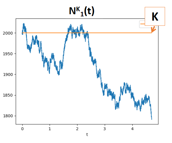
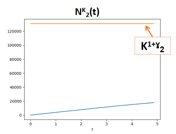
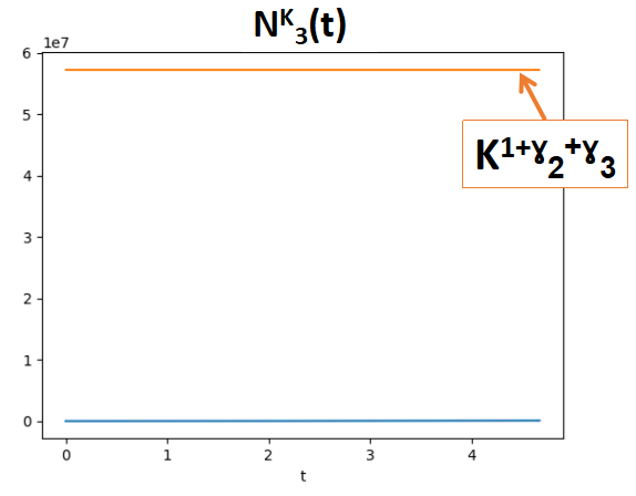
Figure 1: A trajectory of the $N^{K}$ process for $t\in[0,T]$ with $T=O(1)$

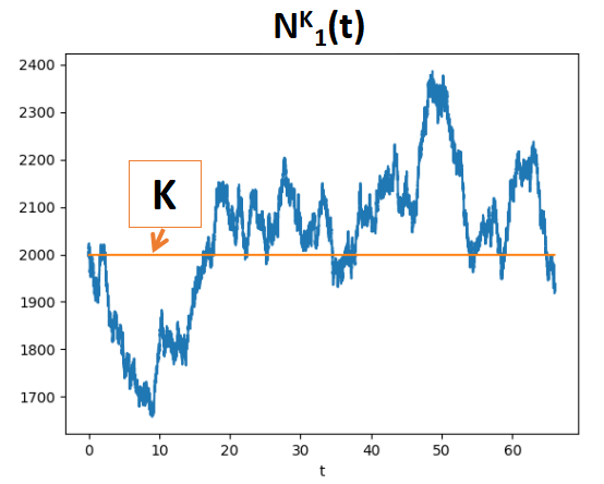
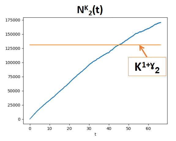
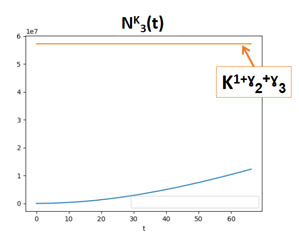
Figure 2: A trajectory of the $N^{K}$ process for $t\in[0,T]$ with $T=O(K^{\gamma_{2}})$

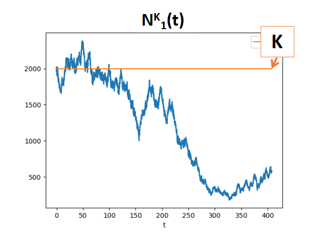
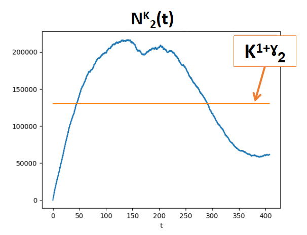
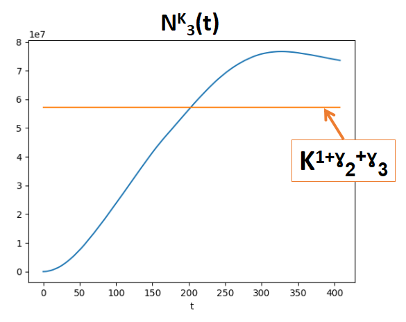
Figure 3: A trajectory of the $N^{K}$ process for $t\in[0,T]$ with $T=O(K^{\gamma_{3}})$

We observe that at a time scale of order $1$, the two last components of the process $N^{K}$ are far from their equilibrium size. We observe in Figure 2 that the two first components of $(N^{K}(t),\quad t\in[0,T])$ for $T\sim K^{\gamma_{2}}$ evolve around their equilibrium size, which is not the case of the third one. In Figure 3, the process is considered on a longer period of time, $T\sim K^{\gamma_{3}}$ and one sees that the third component hits a neighborhood of its equilibrium. Furthermore, we observe the oscillations of the components of $N^{K}$ around their equilibrium. We note that they are smoother and smoother from Compartment 1 to Compartment 3 and that the amplitude of the waves is longer and longer.

Compartment 3 illustrates the particular behavior of the red blood cells in a rest human erythropoiesis, highlighted above. Indeed, the expected variations should be around $K^{-(1+\gamma_{2}+\gamma_{3})/2}\sim 0.01\%$, and we observe variations which seem to be of order $\frac{10^{7}}{K^{(1+\gamma_{2}+\gamma_{3})/2}}\sim 17\%$.

Our aim is to prove and quantify these different behaviors and to explain these large fluctuations.

In Section 2, basic martingale properties are stated, some estimates are given for the moments of compartments sizes and a first study on the convergence of the process at a time-scale of order $1$, when $K$ tends to infinity, is given. We show that the two last components do not reach their equilibrium at this time scale. In Section 3, we study the process on an appropriate time-scale to capture the asymptotic behavior of the second and third types. We show that the limiting behavior of the two first components process at the time scale of order $K^{\gamma_{2}}$ is given by an explicit deterministic function $y$. We also show that this time scale is not long enough to observe the dynamics of the third component. Hence, we study the limiting behavior of the process at the time scale of order $K^{\gamma_{3}}$. At this time scale, the second component process goes too fast and doesn’t converge anymore. We consider the associated occupation measure, as already done in Kurtz [15]. We prove its convergence in a weak sense to the Dirac measure at the unique equilibrium of the second component of the deterministic function $y$. Then we deduce the convergence of the third component to a limiting deterministic system involving this equilibrium. In Section 4, we study and quantify the large fluctuations observed in the simulations. We show that the first component behaves at the different time scales as a Brownian motion. This is not the case for the other two components. Theorem 3 describes the second and third order asymptotics of the second component on its typical time and size scale. The fluctuations around its deterministic limit are not Gaussian. They are described by a finite variation process integrating the randomness of the first component. An independent Brownian motion appears in the third order term. Theorem 4, which is the main theorem of the paper, describes the fluctuations associated with the third component dynamics. We show that the randomness induced by the dynamics of the two last components is negligible. To capture the effect of the randomness of the first component imposes a size-scale which allows to observe the large oscillations of the third component. We identify these oscillations as a finite variation process integrating as above the fluctuations of the first component.

The mathematical modeling of hematopoiesis has been firstly introduced in the seminal paper of Till, McCulloch and Siminovitch [23]. In this paper, the authors study a binary branching process and show, comparing with biological results, that the probabilistic framework is relevant. Since this pioneering work, many mathematical approaches have been proposed to describe more precisely the cell differentiation kinetics, based either on deterministic or stochastic models (a survey concerning many models can be found in [24]). A deterministic approach consists in introducing a dynamical system describing the behavior of the different compartments and in studying different properties of this system, in particular the equilibrium states (see for example [6], [17], [18], [2] and the references therein). One can also add a noise to model some random perturbation of these systems, with an eventual delay (see for example [16], [19]). In [8], a continuous description of the different cells types is also proposed, using a partial differential equation. Moreover, in all these papers, the authors are interested in modeling the regulation which happens when the system is perturbed by some stress and this nonlinearity involves many mathematical difficulties. Let us note that other stochastic models for hematopoiesis have been introduced ([1], [21], [14]) but they concentrate on a specific level (either stem cells or red blood cells). In all this literature, the questions studied by the authors don’t concern the impact of the parameters on the amplification mechanism. We have found only two papers, [7] and [18], in which the question is mentioned. To our knowledge, the fluctuations generated by this amplification mechanism, have never been rigorously studied with such a space-time multiscale point of view.

Most of the slow fast dynamical systems model interaction between species with different behaviors driving the time scales (see for example [13]). In such cases, slow and fast components appear naturally, contrary to our case, for which a fine study is needed to find the specific time scale of each compartment. In the other way, Popovic, Kurtz and Kang in [20] have developed a general theorem for convergence and fluctuations of multiscale processes. Their result can’t explain our asymptotics. Indeed, in their result, the fluctuations around the deterministic behavior of the slow component are Gaussian, which is not the case of the red blood cells dynamics previously described. In their work, the martingale part of the limit is due to two sources of randomness: the slow component dynamics and the averaged effects of the fast components on the slow component dynamics. As previously explained, in our case the randomness of the slow component is only due to the fast ones and its intrinsic randomness is negligible.

Notation. $\mathcal{P}(E)$ and $\mathcal{L}(X)$ will denote respectively the space of probability measures on $E$ and the law of a process $X$. As in [15], we will denote by $l_{m}({\mathbb{R}}_{+})$ the space of measures on $[0,\infty)\times{\mathbb{R}}_{+}$ such that $\mu([0,t]\times{\mathbb{R}}_{+})=t$, for each $t\geq 0$.

2 Amplification mechanism : size-scale dynamics

2.1 The amplification mechanism

As explained in the introduction, we will reduce the model by simplicity to three compartments. The first one will describe the stem cells compartment, the second one will describe the compartment of progenitors and the third one will refer to red blood cells. Also by simplicity, we will describe the type of cells in each compartment by type 1, type 2 and type 3.

Let us now introduce the vector $N^{K}(t)=(N_{1}^{K}(t),N_{2}^{K}(t),N_{3}^{K}(t))$ of population sizes at time $t$. The process $N^{K}$ is a decomposable multi-type branching process, that is a Markov jump process whose dynamics is given by the following equations.

We assume that for any fixed $K$, $N^{K}_{1}(0),N^{K}_{2}(0),N^{K}_{3}(0)$ are integrable.

Let us denote by $(\mathcal{N}_{i}^{j})_{\underset{j\in\{-,+\}}{1\leq i\leq 3}}$ independent Poisson point measures with intensity $dsdu$ on ${\mathbb{R}}_{+}^{2}$ and introduce the filtration $(\mathcal{F}_{t})_{t\geq 0}$ given by

$$\mathcal{F}_{t}=\sigma(\mathcal{N}_{i}^{j}([0,s)\times A);\,i\in\{1,\dots,3\},j\in\{-,+\},\,s\leq t,\,A\in\mathcal{B}({\mathbb{R}^{+}})).$$

Then we have

$$\begin{split}N^{K}_{1}(t)=\,N_{1}^{K}(0)&+\int_{0}^{t}\int_{{\mathbb{R}}_{+}}\bf{1}_{u\leq\frac{\tau_{1}}{2}\,N_{1}^{K}(s^{-})}\,\,\mathcal{N}^{+}_{1}(ds,du)-\int_{0}^{t}\int_{{\mathbb{R}}_{+}}\bf{1}_{u\leq\frac{\tau_{1}}{2}\,N_{1}^{K}(s^{-})}\,\,\mathcal{N}^{-}_{1}(ds,du)\\ N^{K}_{2}(t)=\,N^{K}_{2}(0)&+2\,\int_{0}^{t}\int_{{\mathbb{R}}_{+}}\bf{1}_{u\leq\frac{\tau_{1}}{2}\,N^{K}_{1}(s^{-})}\,\,\mathcal{N}^{-}_{1}(ds,du)+\int_{0}^{t}\int_{{\mathbb{R}}_{+}}\bf{1}_{u\leq\tau_{2}p_{2}^{R}\,N^{K}_{2}(s^{-})}\,\,\mathcal{N}^{+}_{2}(ds,du)\\ &-\int_{0}^{t}\int_{{\mathbb{R}}_{+}}\bf{1}_{u\leq\tau_{2}p_{2}^{D}\,N^{K}_{2}(s^{-})}\,\,\mathcal{N}^{-}_{2}(ds,du)\\ N^{K}_{3}(t)=\,N^{K}_{3}(0)&+2\,\int_{0}^{t}\int_{{\mathbb{R}}_{+}}\bf{1}_{u\leq\tau_{2}p_{2}^{D}\,N^{K}_{2}(s^{-})}\,\,\mathcal{N}^{-}_{2}(ds,du)-\int_{0}^{t}\int_{{\mathbb{R}}_{+}}\bf{1}_{u\leq\tau_{3}K^{-\gamma_{3}}\,N^{K}_{3}(s^{-})}\,\,\mathcal{N}^{-}_{3}(ds,du)\end{split}.$$ (4)

It can be written as

$$\begin{split}\forall t\geq 0,\quad N^{K}_{1}(t)&=\,N^{K}_{1}(0)+M^{K}_{1}(t)\\ N^{K}_{2}(t)&=\,N^{K}_{2}(0)+\tau_{1}\,\int_{0}^{t}N^{K}_{1}(s)\,ds-\tau_{2}\,K^{-\gamma_{2}}\,\int_{0}^{t}N^{K}_{2}(s)\,ds+M^{K}_{2}(t)\\ N^{K}_{3}(t)&=\,N^{K}_{3}(0)+2\,\tau_{2}\,p^{D}_{2}\,\int_{0}^{t}N^{K}_{2}(s)\,ds-\tau_{3}\,K^{-\gamma_{3}}\,\int_{0}^{t}N^{K}_{3}(s)\,ds+M^{K}_{3}(t)\end{split}$$ (5)

where $M^{K}=(M^{K}_{1},M^{K}_{2},M^{K}_{3})$ is a square-integrable martingale such that for all $t\geq 0$,

$$\begin{split}<M^{K}_{1}>_{t}&=\,\tau_{1}\,\int_{0}^{t}N^{K}_{1}(s)\,ds\\ <M^{K}_{2}>_{t}&=\,2\,\tau_{1}\,\int_{0}^{t}N^{K}_{1}(s)\,ds+\tau_{2}\,\int_{0}^{t}N^{K}_{2}(s)\,ds\\ <M^{K}_{3}>_{t}&=\,4\,p^{D}_{2}\tau_{2}\,\int_{0}^{t}N^{K}_{2}(s)\,ds+\tau_{3}K^{-\gamma_{3}}\,\int_{0}^{t}N^{K}_{3}(s)\,ds\\ <M^{K}_{1},M^{K}_{2}>_{t}&=\,-\,\tau_{1}\,\int_{0}^{t}N^{K}_{1}(s)\,ds\\ <M^{K}_{2},M^{K}_{3}>_{t}&=\,-2\,p^{D}_{2}\tau_{2}\,\int_{0}^{t}N^{K}_{2}(s)\,ds.\end{split}$$ (6)

Indeed, by standard localization and Gronwall’s arguments applied to $(N^{K}_{1}(t))_{t}$, we can easily prove that for any $T>0$ and $K\in\mathbb{N}^{*}$,

$${\mathbb{E}}\big{[}\sup_{t\leq T}N^{K}_{1}(t)\big{]}\leq(2+{\mathbb{E}}\big{[}N^{K}_{1}(0)\big{]})e^{2\tau_{1}T},$$ (7)

and then that

$${\mathbb{E}}\big{[}\sup_{t\leq T}N^{K}_{2}(t)\big{]}<+\infty\ ;\ {\mathbb{E}}\big{[}\sup_{t\leq T}N^{K}_{3}(t)\big{]}<+\infty.$$ (8)

We obtain from (5) that the function $t\mapsto n(t)={\mathbb{E}}\big{[}N^{K}(t)\big{]}=(n_{1}(t),n_{2}(t),n_{3}(t))$ satisfies the system of equations

$$\forall t\leq T,\begin{cases}\quad n_{1}(t)&=\,{\mathbb{E}}\big{[}N^{K}_{1}(0)\big{]}\\ \frac{d}{dt}n_{2}(t)&=\,\tau_{1}\,n_{1}(t)-\tau_{2}K^{-\gamma_{2}}\,n_{2}(t)\\ \frac{d}{dt}n_{3}(t)&=\,2\tau_{2}p_{2}^{D}\,n_{2}(t)-\tau_{3}K^{-\gamma_{3}}\,n_{3}(t).\end{cases}$$ (9)

As explained in the introduction,

$${\mathbb{E}}\big{[}N_{1}^{K}(0)\big{]}\sim K.$$ (10)

Therefore there is a unique equilibrium given by

$$\forall t\geq 0,\quad n_{1}^{*} =\,{\mathbb{E}}\big{[}N^{K}_{1}(0)\big{]}\sim K$$

$$n_{2}^{*} =\,\frac{\tau_{1}\,n_{1}^{*}}{\tau_{2}}K^{\gamma_{2}}\sim K^{1+\gamma_{2}}$$

$$n_{3}^{*} =\,\frac{2p^{D}_{2}\tau_{2}\,n_{2}^{*}}{\tau_{3}}K^{\gamma_{3}}\sim K^{1+\gamma_{2}+\gamma_{3}}$$ (11)

Remark 1.

In the above computation, we obtain the order of magnitude of each sub-population size at equilibrium, but we cannot deduce the order of magnitude of the time taken by the process to reach this equilibrium. We will keep this remark in mind in all the paper.

Let us first begin by a lemma showing that for any $K$ and $t$, the expectations of the sub-population sizes behave as expected from (2.1).

Lemma 1.

Let us now assume that

$$\sup_{K}{\mathbb{E}}\big{[}\frac{N^{K}_{1}(0)}{K}\big{]}<+\infty,\quad\sup_{K}{\mathbb{E}}\big{[}\frac{N^{K}_{2}(0)}{K^{1+\gamma_{2}}}\big{]}<+\infty,\quad\sup_{K}{\mathbb{E}}\big{[}\frac{N^{K}_{3}(0)}{K^{1+\gamma_{2}+\gamma_{3}}}\big{]}<+\infty.$$

then

$$\sup_{K,\,t\in{\mathbb{R}}_{+}}{\mathbb{E}}\big{[}\frac{N^{K}_{1}(t)}{K}\big{]}<+\infty\ ,\displaystyle\sup_{K,\,t\in{\mathbb{R}}_{+}}{\mathbb{E}}\big{[}\frac{N^{K}_{2}(t)}{K^{1+\gamma_{2}}}\big{]}<+\infty\ ,\ \displaystyle\sup_{K,\,t\in{\mathbb{R}}_{+}}{\mathbb{E}}\big{[}\frac{N^{K}_{3}(t)}{K^{1+\gamma_{2}+\gamma_{3}}}\big{]}<+\infty.$$

Proof.

The first assertion follows immediately.

From (9), we obtain that for all $t\geq 0$,

$${\mathbb{E}}\big{[}\frac{N^{K}_{2}(t)}{K^{1+\gamma_{2}}}\big{]}=\frac{\tau_{1}}{\tau_{2}}\,{\mathbb{E}}\big{[}\frac{N^{K}_{1}(0)}{K}\big{]}+\big{(}{\mathbb{E}}\big{[}\frac{N^{K}_{2}(0)}{K^{1+\gamma_{2}}}\big{]}-\frac{\tau_{1}}{\tau_{2}}{\mathbb{E}}\big{[}\frac{N^{K}_{1}(0)}{K}\big{]}\big{)}\,e^{-\tau_{2}\,K^{-\gamma_{2}}\,t}$$ (12)

and the proof of the second assertion follows.

Similarly, straightforward computation yields

$${\mathbb{E}}\big{[}\frac{N^{K}_{3}(t)}{K^{1+\gamma_{2}+\gamma_{3}}}\big{]}=\; \frac{2p^{D}_{2}\tau_{1}}{\tau_{3}}\,{\mathbb{E}}\big{[}\frac{N^{K}_{1}(0)}{K}\big{]}-\beta_{K}\,e^{-\tau_{2}\,K^{-\gamma_{2}}\,t}$$ (13)

$$+\Big{(}{\mathbb{E}}\big{[}\frac{N^{K}_{3}(0)}{K^{1+\gamma_{2}+\gamma_{3}}}\big{]}-\frac{2p^{D}_{2}\tau_{1}}{\tau_{3}}\,{\mathbb{E}}\big{[}\frac{N^{K}_{1}(0)}{K}\big{]}+\beta_{K}\Big{)}\,e^{-\tau_{3}\,K^{-\gamma_{3}}\,t},$$

with

$$\beta_{K}={2p^{D}_{2}\tau_{2}}\,\frac{1}{\tau_{2}K^{\gamma_{3}-\gamma_{2}}-\tau_{3}}\Big{(}{\mathbb{E}}\big{[}\frac{N^{K}_{2}(0)}{K^{1+\gamma_{2}}}\big{]}-\frac{\tau_{1}}{\tau_{2}}{\mathbb{E}}\big{[}\frac{N^{K}_{1}(0)}{K}\big{]}\Big{)}.$$

Hence the third assertion is proved.

∎

2.2 Asymptotic behavior on a finite time interval

The parameter $K$ is defined as the order of magnitude of the martingale $N^{K}_{1}$ at time $0$.

The first result describes the dynamics of the process on a finite time interval. The proof of this proposition is left to the reader. It is classical and more difficult proofs in a similar spirit will be given later.

Proposition 1.

Let us introduce the jump process $X^{K}$ defined for all $t\geq 0$ by

$$X^{K}(t)=(\frac{N^{K}_{1}(t)}{K},\frac{N^{K}_{2}(t)}{K^{1+\gamma_{2}}},\frac{N^{K}_{3}(t)}{K^{1+\gamma_{2}+\gamma_{3}}}).$$ (14)

(i) Let us assume that there exists a vector $(x_{1},0,0)\in{\mathbb{R}}_{+}^{3}$ such that the sequence
$\Big{(}\frac{N^{K}_{1}(0)}{K},\frac{N^{K}_{2}(0)}{K^{1+\gamma_{2}}},\frac{N^{K}_{3}(0)}{K^{1+\gamma_{2}+\gamma_{3}}}\Big{)}_{K\in{\mathbb{N}}^{*}}$ converges in law to $(x_{1},0,0)$ when $K$ tends to infinity and such that

$$\sup_{K}{\mathbb{E}}\big{[}\frac{N^{K}_{1}(0)}{K}\big{]}<+\infty,\quad\sup_{K}{\mathbb{E}}\big{[}\frac{N^{K}_{2}(0)}{K^{1+\gamma_{2}}}\big{]}<+\infty\quad\text{ and }\quad\sup_{K}{\mathbb{E}}\big{[}\frac{N^{K}_{3}(0)}{K^{1+\gamma_{2}+\gamma_{3}}}\big{]}<+\infty.$$

Then for all $T>0$, the sequence $(\frac{N^{K}_{1}(t)}{K},\frac{N^{K}_{2}(t)}{K^{1+\gamma_{2}}},\frac{N^{K}_{3}(t)}{K^{1+\gamma_{2}+\gamma_{3}}})_{K\in{\mathbb{N}}^{*}}$ converges in law in $\mathbb{D}([0,T],\mathbb{R}_{+}^{3})$ to $(x_{1},0,0)$.

(ii) Let us assume that there exists a vector $(x_{1},0,0)\in{\mathbb{R}}_{+}^{3}$ such that the sequence
$\Big{(}\frac{N^{K}_{1}(0)}{K},\frac{N^{K}_{2}(0)}{K},\frac{N^{K}_{3}(0)}{K}\Big{)}_{K\in{\mathbb{N}}^{*}}$ converges in law to $(x_{1},0,0)$ when $K$ tends to infinity and such that

$$\sup_{K}{\mathbb{E}}\big{[}\frac{N^{K}_{1}(0)}{K}\big{]}<+\infty,\quad\sup_{K}{\mathbb{E}}\big{[}\frac{N^{K}_{2}(0)}{K}\big{]}<+\infty\quad\text{ and }\quad\sup_{K}{\mathbb{E}}\big{[}\frac{N^{K}_{3}(0)}{K}\big{]}<+\infty.$$

Then for all $T>0$, the sequence $\Big{(}\frac{N^{K}_{1}(t)}{K},\frac{N^{K}_{2}(t)}{K},\frac{N^{K}_{3}(t)}{K}\Big{)}_{K\in{\mathbb{N}}^{*}}$ converges in law in $\mathbb{D}([0,T],\mathbb{R}_{+}^{3})$ to $\ x_{1}\big{(}1,\tau_{1}\,t,{\tau_{2}\over 2}\;t^{2}\big{)}$.

Let us underline that at this time scale, assertion (i) shows that the two last components do not reach their equilibrium order, as observed in the simulations. Assertion (ii) proves that the three compartments are only of order $K$ during the time interval $[0,T]$.

3 Size-time multi-scale dynamics and asymptotic behavior

A size renormalization of the stochastic process is not enough to understand the dynamics of the model. We need to change the time scale as observed in the simulations. This part is devoted to identify and study two significant asymptotics for the process, corresponding to the two time scales $K^{\gamma_{2}}$ and $K^{\gamma_{3}}$, when $K$ is large.

3.1 Asymptotic behavior at a time-scale of order $K^{\gamma_{2}}$

In this section, we study the system composed of the two first components at the time scale $K^{\gamma_{2}}$. To this end, let us introduce the jump process $Y^{K}$ defined for all $t\geq 0$ by

$$Y^{K}(t)=(\frac{N^{K}_{1}(t\,K^{\gamma_{2}})}{K},\frac{N^{K}_{2}(t\,K^{\gamma_{2}})}{K^{1+\gamma_{2}}}).$$ (15)

Let us note that only the time scale differs between processes $X^{K}$ and $Y^{K}$. Hence, at time $t=0$, we have

$$(Y_{1}^{K}(0),Y_{2}^{K}(0))=(X_{1}^{K}(0),X_{2}^{K}(0)).$$

The next theorem describes the approximating behavior of $Y^{K}$ when $K$ tends to infinity.

Theorem 1.

Assume that there exists a vector $(x_{1},x_{2})\in{\mathbb{R}}_{+}^{2}$ such that the sequence $(Y^{K}(0))_{K\in{\mathbb{N}}^{*}}$ converges in law to $(x_{1},x_{2})$ when $K$ tends to infinity and such that

$$\sup_{K}{\mathbb{E}}\big{[}Y^{K}_{1}(0)^{2}+Y^{K}_{2}(0)^{2}\big{]}<\infty.$$

Then for each $T>0$, the sequence $(Y^{K})_{K\in{\mathbb{N}}^{*}}$ converges in law (and hence in probability) in ${\mathbb{D}}([0,T],{\mathbb{R}}_{+}^{2})$ to the continuous function $y=(y_{1},y_{2})$ such that for all $t\geq 0$,

$$\left\{\begin{array}[]{lll}y_{1}(t)&=x_{1}\\ y_{2}(t)&=\frac{\tau_{1}x_{1}}{\tau_{2}}+\big{(}x_{2}-\frac{\tau_{1}x_{1}}{\tau_{2}}\big{)}\,e^{-\tau_{2}\,t}.\end{array}\right.$$ (16)

Proof.

By standard localization argument, use of Gronwall’s Lemma and Doob’s inequality, we easily prove (successively for the first and then for the second component) that for any $T>0$,

$$\displaystyle\sup_{K}{\mathbb{E}}\big{[}\sup_{t\in[0,T]}(Y^{K}_{1}(t)^{2}+Y^{K}_{2}(t)^{2})\big{]}<\infty.$$ (17)

From (5) and (6), we can write

$$Y^{K}_{1}(t) = Y^{K}_{1}(0)+\widehat{M}^{K}_{1}(t)$$

$$Y^{K}_{2}(t) = Y^{K}_{2}(0)+\tau_{1}\int_{0}^{t}Y^{K}_{1}(u)du-\tau_{2}\int_{0}^{t}Y^{K}_{2}(u)du+\widehat{M}^{K}_{2}(t),$$ (18)

where $\widehat{M}^{K}_{1}$ and $\widehat{M}^{K}_{2}$ are two square-integrable martingales satisfying

$$\langle\widehat{M}^{K}_{1}\rangle_{t} = {\tau_{1}\over K^{1-\gamma_{2}}}\int_{0}^{t}Y^{K}_{1}(u)du,$$

$$\langle\widehat{M}^{K}_{2}\rangle_{t} = {2\tau_{1}\over K^{1+\gamma_{2}}}\int_{0}^{t}Y^{K}_{1}(u)du+{\tau_{2}\over K}\int_{0}^{t}Y^{K}_{2}(u)du,$$

$$\langle\widehat{M}^{K}_{1},\widehat{M}^{K}_{2}\rangle_{t} = -{\tau_{1}\over K}\int_{0}^{t}Y^{K}_{1}(u)du.$$ (19)

It is very standard to prove that the sequence of laws of $(Y^{K})$ is tight (using the moment estimates (17)) and that the martingale parts go to $0$. The result follows using the method summarized for example in [4]. Each limiting value is proved to only charge the subset of continuous functions. Then introducing

$$\phi_{t}(y)=\left(\begin{array}[]{c}y_{1}(t)-y_{1}(0)\\ y_{2}(t)-y_{2}(0)-\int_{0}^{t}\big{(}\tau_{1}y_{1}(s)-\tau_{2}y_{2}(s)\big{)}ds\end{array}\right)$$

and using the uniform integrability of the sequence $(\phi_{t}(Y^{K}))_{K}$, deduced from (17), we identify the limit as the unique continuous solution $y$ of the deterministic system defined by $y(0)=(x_{1},x_{2})$ and

$$\forall t\geq 0,\quad\phi_{t}(y)=0.$$

That concludes the proof. ∎

Remark 2.

Since $\gamma_{2}<\gamma_{3}$, the time scale $K^{\gamma_{2}}$ is not large enough to observe the dynamics of the third component. The next proposition shows that at such a time scale, the third component converges to a trivial value.

Proposition 2.

Under the same hypotheses as in Theorem 1, we assume furthermore that there exists $x_{3}\in{\mathbb{R}}_{+}$ such that the sequence $(\frac{N^{K}_{3}(0)}{K^{1+\gamma_{2}+\gamma_{3}}})_{K\in{\mathbb{N}}^{*}}$ converges in law to $x_{3}$ when $K$ tends to infinity and such that

$$\quad\sup_{K}{\mathbb{E}}\big{[}(\frac{N^{K}_{3}(0)}{K^{1+\gamma_{2}+\gamma_{3}}})^{2}\big{]}<\infty.$$

Then for each $T>0$, the sequence $(\frac{N^{K}_{3}(.K^{\gamma_{2}})}{K^{1+\gamma_{2}+\gamma_{3}}})_{K\in{\mathbb{N}}^{*}}$ converges in probability in ${\mathbb{D}}([0,T],{\mathbb{R}}_{+})$ to $x_{3}$.

Proof.

Following (5) and (6), let us write the semimartingale decomposition of the process $\ Y^{K}_{3}=\frac{N^{K}_{3}(.K^{\gamma_{2}})}{K^{1+\gamma_{2}+\gamma_{3}}}$. We have for any $t\leq T$,

$$Y^{K}_{3}(t)=Y^{K}_{3}(0)+2\tau_{2}p^{D}_{2}K^{\gamma_{2}-\gamma_{3}}\int_{0}^{t}Y^{K}_{2}(s)ds-\tau_{3}K^{\gamma_{2}-\gamma_{3}}\int_{0}^{t}Y^{K}_{3}(s)ds+\widehat{M}^{K}_{3}(t),$$ (20)

where $\widehat{M}^{K}_{3}$ is a square-integrable martingale such that

$$\langle\widehat{M}^{K}_{3}\rangle_{t}=2\tau_{2}p^{D}_{2}K^{\gamma_{2}-\gamma_{3}}\int_{0}^{t}Y^{K}_{2}(s)ds+\tau_{3}K^{\gamma_{2}-\gamma_{3}}\int_{0}^{t}Y^{K}_{3}(s)ds.$$

Let us recall that $\gamma_{2}<\gamma_{3}$, which makes $K^{\gamma_{2}-\gamma_{3}}$ tends to $0$ when $K$ tends to infinity.

Using Theorem 1, we know that $Y^{K}_{2}$ converges to the continuous function $y_{2}$. By standard tightness argument, one can easily deduce that the process $Y^{K}_{3}$ converges in probability to $x_{3}$, on any finite time interval. ∎

3.2 Asymptotic behavior at a time-scale of order $K^{\gamma_{3}}$

In order to catch the long time dynamics of the third component we will study the process $N^{K}$ on the time scale $tK^{\gamma_{3}}$. To this end, let us introduce the jump process $Z^{K}$ defined for all $t\geq 0$ by

$$Z^{K}(t)=(\frac{N^{K}_{1}(t\,K^{\gamma_{3}})}{K},\frac{N^{K}_{2}(t\,K^{\gamma_{3}})}{K^{1+\gamma_{2}}},\frac{N^{K}_{3}(t\,K^{\gamma_{3}})}{K^{1+\gamma_{2}+\gamma_{3}}}).$$

Note that we still have

$$Z^{K}(0)=Y^{K}(0)=X^{K}(0).$$

At this time scale, the second component has time to reach the equilibrium of its deterministic approximation by an average procedure. By an adaptation of the proof in [20] to this specific framework, we are able to prove the following theorem.

Theorem 2.

Assume that there exists $(x_{1},x_{2},x_{3})\in{\mathbb{R}}_{+}^{3}$ such that the sequence $(Z^{K}(0))_{K\in{\mathbb{N}}^{*}}$ converges in law to $(x_{1},x_{2},x_{3})$ when $K$ tends to infinity and such that

$$\displaystyle\sup_{K}{\mathbb{E}}\big{[}Z^{K}_{1}(0)\big{]}<+\infty,\quad\sup_{K}{\mathbb{E}}\big{[}Z^{K}_{2}(0)\big{]}<+\infty\quad\text{ and }\quad\sup_{K}{\mathbb{E}}\big{[}Z^{K}_{3}(0)\big{]}<+\infty.$$ (21)

Let $\Gamma^{K}_{2}$ be the $l_{m}({\mathbb{R}}_{+})$-valued random variable given by

$$\Gamma^{K}_{2}([0,t]\times B)=\int_{0}^{t}\bf{1}_{B}(Z^{K}_{2}(s))ds.$$ (22)

Then for all $T>0$, the sequence $(Z^{K}_{1},\Gamma^{K}_{2},Z^{K}_{3})_{K\in{\mathbb{N}}^{*}}$ converges in law in $\mathbb{D}([0,T],{\mathbb{R}}_{+})\times l_{m}({\mathbb{R}}_{+})\times\mathbb{D}([0,T],{\mathbb{R}}_{+})$ to $(z_{1},\delta_{z_{2}^{*}}(dz_{2})\,ds,z_{3})$. The functions $z_{1}$ and $z_{3}$ are defined for all $t\leq T$ by

$$\left\{\begin{array}[]{lll}z_{1}(t)&=x_{1}\\ \\ z_{3}(t)&=\large\frac{\tau_{2}}{\tau_{3}}z^{*}_{2}+\big{(}x_{3}-\frac{\tau_{2}}{\tau_{3}}z^{*}_{2}\big{)}\,e^{-\tau_{3}\,t}\end{array}\right.$$ (23)

and $z_{2}^{*}$ is the value of $y_{2}$ at infinity:

$$z_{2}^{*}=\frac{\tau_{1}x_{1}}{\tau_{2}}.$$

Let us first state a lemma in which all moment estimates are gathered.

Lemma 2.

Under Assumption (21), we obtain

$$\displaystyle\sup_{K}{\mathbb{E}}\big{[}\sup_{t\in[0,T]}Z^{K}_{1}(t)\big{]}<+\infty\ ;\ \quad\forall\,t>0\quad\displaystyle\sup_{K}{\mathbb{E}}\big{[}\int_{0}^{t}Z^{K}_{2}(s)\,ds\big{]}<+\infty\ ;\$$

and

$$\sup_{K}{\mathbb{E}}\big{[}\sup_{t\in[0,T]}Z^{K}_{3}(t)\big{]}<+\infty.$$

Proof of Lemma 2.

The first and third estimates are obtained by usual arguments (localization, Doob’s inequality and Gronwall’s Lemma). Let us focus on the second one.

By positivity and definition of the process $Z^{K}_{2}$, we have for any $t>0$

$$Z^{K}_{2}(t)=Z^{K}_{2}(0)+\tau_{1}K^{\gamma_{3}-\gamma_{2}}\int_{0}^{t}Z^{K}_{1}(s)ds-\tau_{2}K^{\gamma_{3}-\gamma_{2}}\int_{0}^{t}Z^{K}_{2}(s)ds+\widetilde{M}^{K}_{2}(t),$$ (24)

the latter term being a square-integrable martingale and

$$\langle\widetilde{M}^{K}_{2}\rangle_{t}=\frac{1}{K^{1+\gamma_{2}}}\Big{(}2\tau_{1}K^{\gamma_{3}-\gamma_{2}}\int_{0}^{t}Z^{K}_{1}(s)ds+\tau_{2}K^{\gamma_{3}}\int_{0}^{t}Z^{K}_{2}(s)ds\Big{)}.$$ (25)

In particular,

$${\mathbb{E}}\big{[}\int_{0}^{t}Z^{K}_{2}(s)\,ds\big{]}={1\over\tau_{2}}K^{\gamma_{2}-\gamma_{3}}\Big{(}{\mathbb{E}}\big{[}Z^{K}_{2}(0)\big{]}-{\mathbb{E}}\big{[}Z^{K}_{2}(t)\big{]}\Big{)}+{\tau_{1}\over\tau_{2}}\int_{0}^{t}{\mathbb{E}}\big{[}Z^{K}_{1}(s)\big{]}\,ds.$$

Assumptions (21) and Lemma 1 ensure that the first term goes to $0$ as $K$ tends to infinity and the third term is bounded uniformly in $K$. That allows to conclude. ∎

Proof of Theorem 2.

Let $\Gamma^{K}$ be the occupation measure of $Z^{K}$, a random measure belonging to the space $l_{m}({\mathbb{R}}_{+})$ of positive measures on $[0,\infty)\times{\mathbb{R}}_{+}$ with mass $t$ on$[0,t]\times{\mathbb{R}}_{+}$ and defined for all Borelian set $B$ and for $t>0$ by

$$\Gamma^{K}([0,t]\times B)=\int_{0}^{t}\bf{1}_{B}(Z^{K}(s))\,ds.$$

Using Lemma 2.9 of [20] (cf. Appendix), we obtain that $(\Gamma^{K})_{K}$ is relatively compact in $l_{m}({\mathbb{R}}_{+})$ endowed with a weak topology generated by the class of test functions defined in (52) .

Let us denote by $\Gamma\in l_{m}({\mathbb{R}}_{+}^{3})$ a limiting value. Using [15] Lemma 1.4, one can show that there exists a $\mathcal{P}({\mathbb{R}}_{+}^{3})$-valued process $\gamma_{s}$ such that

$$\Gamma(dz\times ds)=\gamma_{s}(dz)\,ds.$$

Let us now introduce the function $F^{K}$

$$\forall z\in{\mathbb{R}}_{+}^{3},\quad F^{K}(z)=(1+{1\over K^{\gamma_{2}}})\,\tau_{2}z_{2}-\tau_{3}\,z_{3}.$$

Then for all $t\geq 0$,

$$\quad Z^{K}_{3}(t) =Z^{K}_{3}(0)+(1+{1\over K^{\gamma_{2}}})\tau_{2}\int_{0}^{t}Z^{K}_{2}(s)ds-\tau_{3}\,\int_{0}^{t}Z^{K}_{3}(s)ds+\widetilde{M}^{K}_{3}(t)$$ (26)

$$=Z^{K}_{3}(0)+\int_{0}^{t}F^{K}(Z^{K}(s))\,ds+\widetilde{M}^{K}_{3}(t)$$

$$Z^{K}_{1}(t) =Z^{K}_{1}(0)+\widetilde{M}^{K}_{1}(t)$$ (27)

with $(\widetilde{M}^{K}_{1},\widetilde{M}^{K}_{3})$ independent martingales and such that for all $t\geq 0$,

$$<\widetilde{M}^{K}_{1}>_{t}= K^{\gamma_{3}-1}\,\int_{0}^{t}2\tau_{1}\,Z^{K}_{1}(s)\,ds$$ (28)

$$<\widetilde{M}^{K}_{3}>_{t}= K^{-(1+\gamma_{2}+\gamma_{3})}\,\int_{0}^{t}\big{(}2(1+{1\over K^{\gamma_{2}}})\tau_{2}\,Z^{K}_{2}(s)+\tau_{3}Z^{K}_{3}(s)\big{)}\,ds.$$ (29)

By usual arguments involving Lemma 2 one can prove that the sequences of processes $(Z^{K}_{3})_{K}$ and $(Z^{K}_{1})_{K}$ are uniformly tight in $\mathbb{D}([0,T],{\mathbb{R}}_{+})$. Let us also note that the distributions of any limiting value only charge processes with a.s. continuous trajectories.

Furthermore by Doob’s inequality

$${\mathbb{E}}\big{[}\sup_{t\leq T}|\widetilde{M}^{K}_{3}(t)|^{2}\big{]}\leq 4\,{\mathbb{E}}\big{[}<\widetilde{M}^{K}_{3}>_{T}\big{]}.$$

Using (29) and Lemma 2, we obtain that $\ \lim_{K\to\infty}{\mathbb{E}}\big{[}\sup_{t\in[0,T]}|\widetilde{M}^{K}_{3}(t)|^{2}\big{]}=0$ and a similar property for $\widetilde{M}^{K}_{1}$ since $\gamma_{3}<1$. Then, we deduce from Markov’s inequality, that the processes $(\widetilde{M}^{K}_{3})_{K}$ and $(\widetilde{M}^{K}_{1})_{K}$ converge in probability for the uniform norm to 0. Hence they converge in law in $\mathbb{D}([0,T],{\mathbb{R}}_{+})$ to $0$.

Adding all these asymptotic behaviors, we deduce that there exists a subsequence of $(Z^{K}_{1},Z^{K}_{3})$ converging in law in ${\mathbb{D}}([0,T],{\mathbb{R}}_{+}^{2})$ to the deterministic limit $(z_{1},Z_{3}^{\infty})$ defined for all $t\geq 0$ by

$$\,\quad z_{1}(t) =x_{1}$$

$$Z_{3}^{\infty}(t) =x_{3}+\int_{{\mathbb{R}}_{+}^{3}\times[0,t]}(\,\tau_{2}z_{2}-\tau_{3}\,z_{3})\gamma_{s}(dz)ds.$$

Then by convergence of $(Z^{K}_{1})_{K}$, $(Z^{K}_{3})_{K}$ and $\Gamma^{K}$, one can easily deduce that

$$\gamma_{s}(dz)=\delta_{\bar{z}_{1}}(dz_{1})\delta_{Z^{\infty}_{3}(s)}(dz_{3})\,\tilde{\gamma}_{s}(z_{1},z_{3},dz_{2}).$$

We have now to identify these measures $\tilde{\gamma}_{s},\ s\in[0,T]$.

Let us write the generator of the process $Z^{K}_{2}$. For $h\in C^{\infty}_{c}$ , it is given for $z\in{\mathbb{R}}_{+}^{3}$ by

$$\mathcal{L}^{K}_{2}(h)(z)= \big{(}h(z_{2}+2\,K^{-(1+\gamma_{2})})-h(z_{2})\big{)}\,\frac{\tau_{1}}{2}\,z_{1}\,K^{1+\gamma_{3}}$$

$$+\big{(}h(z_{2}+\,K^{-(1+\gamma_{2})})-h(z_{2})\big{)}\,p^{R}_{2}\tau_{2}\,z_{2}\,K^{1+\gamma_{2}+\gamma_{3}}$$

$$+\big{(}h(z_{2}-\,K^{-(1+\gamma_{2})})-h(z_{2})\big{)}\,p^{D}_{2}\tau_{2}\,z_{2}\,K^{1+\gamma_{2}+\gamma_{3}}.$$

Let us introduce the function $g$ defined for $z\in{\mathbb{R}}_{+}^{3}$ by

$$\quad g(z)=\,z_{1}\tau_{1}-\tau_{2}z_{2}.$$

Then, by a Taylor expansion, we obtain that

$$\forall h\in C^{\infty}_{c},\quad\lim_{K\to\infty}\sup_{z\in{\mathbb{R}}_{+}}|K^{\gamma_{2}-\gamma_{3}}\mathcal{L}^{K}_{2}(h)(z)-g(z)h^{\prime}(z_{2})|=0.$$ (30)

Using (25), Lemma 3 and the same arguments as above, we obtain that the sequence of processes $\Big{(}K^{\gamma_{2}-\gamma_{3}}\,\Big{(}h(Z^{K}_{2}(t))-h(Z^{K}_{2}(0))-\int_{0}^{t}\mathcal{L}_{2}^{K}(h)(Z^{K}(s))\,ds\Big{)},\quad t\in[0,T]\Big{)}$ converges in law in ${\mathbb{D}}([0,T],{\mathbb{R}})$ to $0$. In the other hand, using that $h$ is bounded and (30) and $g\,h^{\prime}\in C_{b}$ (since $h$ has compact support), we easily see that this sequence also converges to

$$-\int_{0}^{t}(\tau_{1}x_{1}-\tau_{2}z_{2})h^{\prime}(z_{2})\,\gamma_{s}(z_{1},z_{3},dz_{2})\,ds.$$

We deduce that for any $t\in[0,T]$, for any $h\in C^{\infty}_{c}$

$$\int_{0}^{t}(\tau_{1}x_{1}-\tau_{2}z_{2})h^{\prime}(z_{2})\,\tilde{\gamma}_{s}(z_{1},z_{3},dz_{2})\,ds=0.$$

It implies that

$$\tilde{\gamma}_{s}(z_{1},z_{3},dz_{2})=\delta_{\frac{\tau_{1}x_{1}}{\tau_{2}}}(dz_{2}).$$

To end the proof, we solve the equation satisfied by $Z^{\infty}_{3}(t)$ and obtain that

$$\forall t\geq 0,\quad Z^{\infty}_{3}(t)=\frac{\tau_{1}x_{1}}{\tau_{3}}+\big{(}x_{3}-\frac{\tau_{1}x_{1}}{\tau_{3}}\big{)}\,e^{-\tau_{3}\,t}.$$

Hence we have uniquely identified the limit of any converging subsequence. That ends the proof.

∎

4 Amplified fluctuations

In this section, we will quantify the large fluctuations observed on the simulations. As pointed out above, each component has its own typical size and time scale. Hence, we will study separately the fluctuations of the second and third types. Classical results easily imply that the first component behaves as a Brownian motion: for large $K$, for all $t\in[0,T]$,

$$N^{K}_{1}(t)\sim x_{1}\,K+\sqrt{K}\,\sqrt{\tau_{1}x_{1}}\,B_{t}.$$

The originality of our results concerns the large fluctuations of the two last types due to the amplification of these first type fluctuations.

4.1 The large fluctuations of the second type

As seen in Subsection 3.1, the typical size scale (respectively time scale) of the second type is $K^{1+\gamma_{2}}$ (respectively $K^{\gamma_{2}}$) and the first order asymptotics relative to this time scale is given by the function $y$ defined by (16). We are also able to give an expansion of the process at the second and third orders on such time scale.

Theorem 3.

Let define the sequence $(U^{K})_{K}$ by

$$\forall t\geq 0,\quad U^{K}(t)=K^{(1-\gamma_{2})/2}\big{(}Y^{K}(t)-y(t)\big{)}.$$

(i) Assume that there exists $U_{0}=(U_{0}^{(1)},U_{0}^{(2)})\in{\mathbb{R}}^{2}$ such that $(U^{K}(0))_{K\in{\mathbb{N}}^{*}}$ converges in law to $U_{0}$ and that

$$\displaystyle\sup_{K}{\mathbb{E}}\big{[}U^{K}_{1}(0)^{2}+U^{K}_{2}(0)^{2}\big{]}<+\infty.$$ (31)

Then for each $T>0$, the sequence $(U^{K})_{K\in{\mathbb{N}}^{*}}$ converges in law in ${\mathbb{D}}([0,T],{\mathbb{R}}^{2})$ to the process $U=(U_{1},U_{2})$ defined for all $t\geq 0$ by

$$U_{1}(t) = U_{0}^{(1)}+\sqrt{\tau_{1}\,x_{1}}\,B_{1}(t),$$ (32)

$$U_{2}(t) = U_{0}^{(2)}+\tau_{1}\int_{0}^{t}U_{1}(s)ds-\tau_{2}\int_{0}^{t}U_{2}(s)\,ds,$$ (33)

where $B_{1}$ is a standard Brownian motion.

(ii) Furthermore, the sequence $(W^{K}_{2})_{K\in{\mathbb{N}}^{*}}$ defined by

$$\forall t\in[0,T],\quad W^{K}_{2}(t)=K^{\gamma_{2}/2}\;\big{[}U^{K}_{2}(t)-U_{0}^{(2)}-\tau_{1}\int_{0}^{t}U_{1}^{K}(s)ds+\tau_{2}\int_{0}^{t}U^{K}_{2}(s)ds\big{]},$$

converges in law in ${\mathbb{D}}([0,T],{\mathbb{R}})$, for each $T>0$, to the process $(\sqrt{\tau_{2}y_{2}(t)}\,B_{2}(t),\quad t\in[0,T])$ where $B_{2}$ is a standard Brownian motion independent of the process $B_{1}$.

From this theorem, we can deduce the following expansion, which quantifies the large waves of fluctuations. Assuming that $U_{0}$ is equal to zero, we obtain for all $t$ and large $K$,

$$N_{2}^{K}(t)\sim K^{1+\gamma_{2}}y_{2}(t\,K^{-\gamma_{2}})+K^{(1+3\gamma_{2})/2}U_{2}(t\,K^{-\gamma_{2}})+K^{(1+2\gamma_{2})/2}\sqrt{\tau_{2}\,y_{2}(t\,K^{-\gamma_{2}})}\,B_{2}(t\,K^{-\gamma_{2}})$$

where

$$\forall t,\quad U_{2}(t)=\tau_{1}\sqrt{\tau_{1}x_{1}}\int_{0}^{t}B_{1}(s)\,ds-\tau_{2}\int_{0}^{t}U_{2}(s)\,ds$$

and $B_{1}$, $B_{2}$ are independent Brownian motions.

Proof of Theorem 3..

(i) First we deduce from (31) with similar arguments as above that

$$\displaystyle\sup_{K}{\mathbb{E}}\big{[}\sup_{t\in[0,T]}(U^{K}_{1}(t)^{2}+U^{K}_{2}(t)^{2})\big{]}<+\infty.$$ (34)

The tightness of the families $(\displaystyle\sup_{t\leq T}|U^{K}_{1}(t)|)_{K}$ and $(\displaystyle\sup_{t\leq T}|U^{K}_{2}(t)|)_{K}$ immediately follows.

We consider the semi-martingale decomposition of $(U^{K})$ and write

$$U^{K}_{i}(t)=U^{K}_{i}(0)+A^{K}_{i}(t)+K^{\frac{1-\gamma_{2}}{2}}\widehat{M}^{K}_{i}(t),$$

where $\widehat{M}^{K}$ has been defined in (3.1), $A^{K}_{1}=0$ and $A^{K}_{2}(t)=\tau_{1}\int_{0}^{t}U^{K}_{1}(s)\,ds-\tau_{2}\int_{0}^{t}U_{2}^{K}(s)\,ds$.

Thanks to the above moment estimates, it is almost immediate to prove that the finite variation processes $<K^{\frac{1-\gamma_{2}}{2}}\widehat{M}^{K}_{i}>$ and $A^{K}_{2}$ satisfy the Aldous condition. Thanks to Aldous and Rebolledo criteria (see [12] and [4]) , the uniform tightness of $\mathcal{L}(U^{K})$ in $\mathcal{P}({\mathbb{D}}([0,T],{\mathbb{R}}^{2}))$ follows.

We denote by simplicity by the same notation $(U^{K})_{K}$ a subsequence converging in law in ${\mathbb{D}}([0,T],{\mathbb{R}}^{2})$. Let $Q$ be the limiting value of $(\mathcal{L}(U^{K}))_{K}$. It is easy to observe that

$$\sup_{t\in[0,T]}\parallel\Delta U^{K}(t)\parallel\leq 2K^{-(1+\gamma_{2})/2}.$$

Therefore, by continuity of the mapping $x\to\displaystyle\sup_{t\in[0,T]}\parallel\Delta x(t)\parallel$ from ${\mathbb{D}}([0,T],{\mathbb{R}}^{2})$ into ${\mathbb{R}}_{+}$, the probability measure $Q$ only charges the processes with continuous paths.

The extended generator of $U^{K}$ is defined for functions $f\in C^{2}_{b}({\mathbb{R}}^{2},{\mathbb{R}})$ as: $\forall u\in{\mathbb{R}}^{2}$,

$$\begin{split}\mathcal{L}^{K}(f,t)(u)&=\big{(}f(u_{1}+K^{-(1+\gamma_{2})/2},u_{2})-f(u)\big{)}\,\frac{\tau_{1}}{2}\,K^{1+\gamma_{2}}(K^{-(1-\gamma_{2})/2}u_{1}+x_{1})\\ +&\big{(}f(u_{1}-\,K^{-(1+\gamma_{2})/2},u_{2}+2K^{-(1+3\gamma_{2})/2})-f(u)\big{)}\,\frac{\tau_{1}}{2}\,K^{1+\gamma_{2}}(K^{-(1-\gamma_{2})/2}u_{1}+x_{1})\\ +&\big{(}f(u_{1},u_{2}+K^{-(1+3\gamma_{2})/2})-f(u)\big{)}\,p^{R}_{2}\,\tau_{2}\,K^{1+2\gamma_{2}}(K^{-(1-\gamma_{2})/2}u_{2}+y_{2}(t))\\ +&\big{(}f(u_{1},u_{2}-K^{-(1+3\gamma_{2})/2})-f(u)\big{)}\,p^{D}_{2}\,\tau_{2}\,K^{1+2\gamma_{2}}(K^{-(1-\gamma_{2})/2}u_{2}+y_{2}(t))\\ -&K^{(1-\gamma_{2})/2}\partial_{2}f(u)\big{(}\tau_{1}x_{1}-\tau_{2}y_{2}(t)\big{)}.\end{split}$$ (35)

By a Taylor’s expansion, we easily obtain that $\forall f\in C^{2}_{b}({\mathbb{R}}^{2},{\mathbb{R}})$,

$$\lim_{K\to\infty}\sup_{(u,t)\in{\mathbb{R}}\times{\mathbb{R}}_{+}}\big{|}\mathcal{L}^{K}(f,t)(u)-(\frac{\tau_{1}}{2}x_{1}\partial_{1}^{2}f(u)+(\tau_{1}u_{1}-\tau_{2}u_{2})\partial_{2}f(u))\big{|}=0.$$ (36)

In the other hand, let us define, for $f\in C^{2}_{b}({\mathbb{R}}^{2},{\mathbb{R}})$, $u\in{\mathbb{D}}([0,T],{\mathbb{R}}^{2})$ and $t\in[0,T]$, the function $\xi^{K,f}_{t}$ by

$$\xi^{K,f}_{t}(u)=f(u_{t})-f(u_{0})-\int_{0}^{t}\mathcal{L}^{K}(f,s)(u_{s})\,ds.$$

Then, by (35), Dynkin’s formula and (34), we can easily prove that the processes $(\xi_{t}^{K,f}(U^{K}))_{K}$ are uniformly integrable martingales.

Therefore by standard arguments (cf. [9], [4]), the limiting process under $Q$ is continuous and satisfies the following martingale problem:

$$\forall f\in C^{2}_{b}({\mathbb{R}}^{2},{\mathbb{R}}),\quad f(U(t))-f(U_{0})-\int_{0}^{t}(\frac{\tau_{1}}{2}x_{1}\partial_{1}^{2}f(U(s))+(\tau_{1}U_{1}(s)-\tau_{2}U_{2}(s))\partial_{2}f(U(s)))\,ds$$

is a martingale.

We conclude using a representation theorem (cf. [11] p.84) that for each $T>0$, the sequence $(U^{K})_{K\in{\mathbb{N}}^{*}}$ converges in law in ${\mathbb{D}}([0,T],{\mathbb{R}}^{2})$ to the process $U=(U_{1},U_{2})$, unique solution of the following stochastic differential system: for all $t\in[0;T]$,

$$U_{1}(t) = U_{0}^{(1)}+\sqrt{\tau_{1}\,x_{1}}\,B_{1}(t),$$

$$U_{2}(t) = U_{0}^{(2)}+\tau_{1}\int_{0}^{t}U_{1}(s)ds-\tau_{2}\int_{0}^{t}U_{2}(s)\,ds,$$

with $B_{1}$ a Brownian motion.

(ii) Let us now expand the second component to the next order. We deduce from (3.1) that

$$U^{K}_{1}(.)-U^{K}(0) = K^{(1-\gamma_{2})/2}\,\widehat{M}^{K}_{1}(.),$$

$$W^{K}_{2}(.) = \sqrt{K}\,\widehat{M}^{K}_{2}(.).$$

Using (3.1), (17) and applying Theorem 7.1.4 of [9], we conclude the proof. ∎

4.2 The large fluctuations of the third type

Let us now study the fluctuation process associated with the largest fluctuation scale of the third component. We have seen in Theorem 2 that at the time scale $K^{\gamma_{3}}$, the size of the population process in the third compartment is of order of magnitude $K^{1+\gamma_{2}+\gamma_{3}}$. In an usual setting, the Central Limit Theorem would lead to fluctuations of order $K^{(1+\gamma_{2}+\gamma_{3})/2}$. We will see in the next theorem that they are of order $K^{(1+2\gamma_{2}+3\gamma_{3})/2}\gg K^{(1+\gamma_{2}+\gamma_{3})/2}$, since amplified by the fluctuations of the first compartment.

Using (23), (24) and (26), we know that for all $t\geq 0$,

$$\big{(}Z_{3}^{K}(t)-z_{3}(t)\big{)} =\big{(}Z_{3}^{K}(0)-z_{3}(0)\big{)}+\tau_{2}\int_{0}^{t}\big{(}Z_{2}^{K}(s)-z_{2}^{*}\big{)}ds-\tau_{3}\,\int_{0}^{t}\big{(}Z_{3}^{K}(s)-z_{3}(s)\big{)}ds$$

$$\quad+\tau_{2}\frac{1}{K^{\gamma_{2}}}\int_{0}^{t}\big{(}Z_{2}^{K}(s)-z_{2}^{*}\big{)}ds+\widetilde{M}^{K}_{3}(t)$$ (37)

where

$$\big{(}Z_{2}^{K}(t)-z_{2}^{*}\big{)} =\big{(}Z_{2}^{K}(0)-z_{2}^{*}\big{)}+K^{\gamma_{3}-\gamma_{2}}\tau_{1}\int_{0}^{t}\big{(}Z_{1}^{K}(s)-x_{1}\big{)}ds$$

$$\quad-K^{\gamma_{3}-\gamma_{2}}\tau_{2}\,\int_{0}^{t}\big{(}Z_{2}^{K}(s)-z_{2}^{*}\big{)}ds+\widetilde{M}^{K}_{2}(t).$$ (38)

Our goal is to quantify the effect of the first component fluctuations on the dynamics of the third component. Considering the expressions of the martingale quadratic variation (28) imposes the choice of the rescaling parameter $K^{(1-\gamma_{3})/2}$ in front of $\big{(}Z_{1}^{K}(t)-x_{1}\big{)}$. We will see that to keep the effect of the first component on the third component, we need to rescale $\big{(}Z_{2}^{K}(t)-Z_{2}^{K}(0)\big{)}$ by $\frac{K^{(1-\gamma_{3})/2}}{K^{\gamma_{3}-\gamma_{2}}}$ and $\big{(}Z_{3}^{K}(t)-z_{3}(t)\big{)}$ by $K^{(1-\gamma_{3})/2}$.

Let us now state the main theorem of this section.

Theorem 4.

Let us define the three processes

$$\forall t\geq 0,\quad\left\{\begin{array}[]{lll}V_{1}^{K}(t)&=K^{(1-\gamma_{3})/2}\big{(}Z_{1}^{K}(t)-x_{1}\big{)}\\ \\ V_{2}^{K}(t)&=\frac{K^{(1-\gamma_{3})/2}}{K^{\gamma_{3}-\gamma_{2}}}\big{(}Z_{2}^{K}(t)-Z_{2}^{K}(0)\big{)}\\ \\ V_{3}^{K}(t)&=K^{(1-\gamma_{3})/2}\big{(}Z_{3}^{K}(t)-z_{3}(t)\big{)}\end{array}\right..$$

Let us assume that there exists $V_{0}=(V_{0}^{(1)},V_{0}^{(3)})$ a ${\mathbb{R}}^{2}$-valued random vector such that the sequence $(V_{1}^{K}(0),V_{3}^{K}(0))_{K\in{\mathbb{N}}^{*}}$ converges in law to $V_{0}$ and such that

$$\displaystyle\sup_{K}{\mathbb{E}}\big{[}V^{K}_{1}(0)^{4}\big{]}<+\infty\quad;\quad\sup_{K}{\mathbb{E}}\big{[}Z_{2}^{K}(0)^{2}\big{]}<+\infty.$$ (39)

$$\sup_{K}{\mathbb{E}}\big{[}|V^{K}_{3}(0)|\big{]}<+\infty.$$ (40)

Then for all $T>0$, the sequence $(V^{K}_{1},V^{K}_{3})_{K\in{\mathbb{N}}^{*}}$ converges in law in $\mathbb{D}([0,T],{\mathbb{R}}^{2})$ to $(V_{1},V_{3})$ such that for all $t$,

$$V_{1}(t)=V_{0}^{(1)}+\sqrt{\tau_{1}\,x_{1}}W_{1}(t)$$

$$V_{3}(t)=V_{0}^{(3)}+\tau_{1}\int_{0}^{t}V_{1}(s)ds-\tau_{3}\int_{0}^{t}V_{3}(s)\,ds,$$

where $W_{1}$ is a standard Brownian motion.

Let us interpret this result in terms of fluctuations. Assuming that the initial vector $V_{0}$ is equal to zero, we obtain that for any $t$ and large $K$,

$$N_{3}^{K}(t)\sim K^{1+\gamma_{2}+\gamma_{3}}\,z_{3}(t\,K^{-\gamma_{3}})+K^{(1+2\gamma_{2}+3\gamma_{3})/2}\,V_{3}(t\,K^{-\gamma_{3}})$$ (41)

where

$$\forall t,\quad V_{3}(t)=\tau_{1}\sqrt{\tau_{1}x_{1}}\int_{0}^{t}W_{1}(s)\,ds-\tau_{3}\int_{0}^{t}V_{3}(s)\,ds$$

and $W_{1}$ is a standard Brownian motion.

The order of magnitude appearing in the fluctuation second order term (41) summarizes the cumulative effects of the third dynamics driven by the fluctuations of the first level. That can explain the exceptionally large fluctuations observed for the size of terminal cells populations, in hematopoietic systems.

As a first step in the proof of Theorem 4, we will prove that the sequence of processes $(V^{K}_{2})_{K}$ converges to $0$ uniformly in $\mathbb{L}^{2}$ on any finite time interval.

Proposition 3.

Under the assumption (39), we obtain

$$\forall T\geq 0,\quad\lim_{K\to\infty}{\mathbb{E}}\big{[}\sup_{t\in[0,T]}V^{K}_{2}(t)^{2}\big{]}=0.$$ (42)

Proof.

Using (24), we obtain that

$$\forall t\geq 0,\quad V^{K}_{2}(t) =K^{\frac{1-3\gamma_{3}}{2}+\gamma_{2}}\big{(}Z^{K}_{2}(t)-Z^{K}_{2}(0)\big{)}$$

$$=\tau_{1}\int_{0}^{t}V_{1}^{K}(s)\,ds-\tau_{2}\,K^{\gamma_{3}-\gamma_{2}}\int_{0}^{t}V^{K}_{2}(s)\,ds+\mathcal{R}^{K}(t),$$

where $\mathcal{R}^{K}$ is the square-integrable martingale defined by

$$\forall t\geq 0,\quad\mathcal{R}^{K}_{t}=K^{\frac{1-3\gamma_{3}}{2}+\gamma_{2}}\widetilde{M}^{K}_{2}(t)$$ (43)

and satisfying

$$\forall t,\quad\langle\mathcal{R}^{K}\rangle_{t}=\,K^{-2\gamma_{3}}\Big{(}\tau_{1}\,\int_{0}^{t}Z^{K}_{1}(s)\,ds+\tau_{2}\,K^{\gamma_{2}}\int_{0}^{t}Z^{K}_{2}(s)\,ds\Big{)}.$$ (44)

Let us first show that

$$\forall t>0,\quad\sup_{K}{\mathbb{E}}\big{[}\int_{0}^{t}V^{K}_{2}(s)^{4}\,ds\big{]}<\infty.$$

Itô’s formula immediately implies that $\forall t\geq 0$,

$$V^{K}_{2}(t)^{4} =V^{K}_{2}(0)^{4}+4\,\int_{0}^{t}V_{2}^{K}(s)^{3}\,d\mathcal{R}^{K}_{s}+4\,\int_{0}^{t}V_{2}^{K}(s)^{3}\,\big{(}\tau_{1}V_{1}^{K}(s)-K^{\gamma_{3}-\gamma_{2}}\tau_{2}V^{K}_{2}(s)\big{)}\,ds$$

$$\quad\quad+6\,\int_{0}^{t}V_{2}^{K}(s)^{2}\,d\langle\mathcal{R}^{K}\rangle_{s}.$$

By standard localization arguments, we prove using (39) that for any $t\geq 0$,

$$\forall t\geq 0,\quad\sup_{K}{\mathbb{E}}\big{[}\int_{0}^{t}V^{K}_{1}(s)^{4}\,ds\big{]}<\infty.$$ (45)

Let us now introduce the stopping time

$$T_{n}=\inf\{t\geq 0,|V^{K}_{2}(t)|\geq n\}.$$

Then, applying the following inequality

$$4\big{(}\tau_{1}v_{1}v_{2}-K^{\gamma_{3}-\gamma_{2}}\tau_{2}v_{2}^{2}\big{)} =4\,\tau_{2}K^{\gamma_{3}-\gamma_{2}}\big{(}[\frac{v_{1}\tau_{1}}{2\tau_{2}\,K^{\gamma_{3}-\gamma_{2}}}]^{2}-[v_{2}-\frac{v_{1}\tau_{1}}{2\tau_{2}\,K^{\gamma_{3}-\gamma_{2}}}]^{2}\big{)}$$

$$\leq\,\frac{v_{1}^{2}\tau_{1}^{2}}{\tau_{2}\,K^{\gamma_{3}-\gamma_{2}}}$$ (46)

to $v_{1}=V_{1}^{K}(s)$ and $v_{2}=V_{2}^{K}(s)$, we obtain the following upper-bound.

$${\mathbb{E}}\big{[}V^{K}_{2}({t\wedge T_{n}})^{4}\big{]}\leq{\mathbb{E}}\big{[}V^{K}_{2}(0)^{4}\big{]} +\,\frac{\tau_{1}^{2}}{\tau_{2}\,K^{\gamma_{3}-\gamma_{2}}}\int_{0}^{t\wedge T_{n}}{\mathbb{E}}\big{[}V_{2}^{K}(s)^{2}\,V_{1}^{K}(s)^{2}\big{]}ds$$

$$+6\,{\mathbb{E}}\big{[}\int_{0}^{t\wedge T_{n}}V_{2}^{K}(s)^{2}\,d\langle\mathcal{R}^{K}\rangle_{s}\big{]}.$$ (47)

Using (44), we obtain for all $t\in[0,T]$,

$${\mathbb{E}}\big{[}\int_{0}^{t\wedge T_{n}}V_{2}^{K}(s)^{2}\,d\langle\mathcal{R}^{K}\rangle_{s}\big{]}=K^{\gamma_{2}-2\gamma_{3}}\,{\mathbb{E}}\big{[}\int_{0}^{t\wedge T_{n}}V_{2}^{K}(s)^{2}\,\big{(}K^{-\gamma_{2}}\tau_{1}Z^{K}_{1}(s)+\tau_{2}Z^{K}_{2}(s)\big{)}\,ds\big{]}.$$

Writing $Z_{2}^{K}$ in function of $V_{2}^{K}$, we find the following upper bound,

$${\mathbb{E}}\big{[}\int_{0}^{t\wedge T_{n}}V_{2}^{K}(s)^{2}\,d\langle\mathcal{R}^{K}\rangle_{s}\big{]} \leq\big{(}\tau_{1}K^{-2\gamma_{3}}+\tau_{2}K^{-(1+\gamma_{3})/2}+\tau_{2}K^{\gamma_{2}-2\gamma_{3}}\big{)}\int_{0}^{t\wedge T_{n}}{\mathbb{E}}\big{[}V_{2}^{K}(s)^{4}\big{]}\,ds$$

$$+\tau_{1}K^{-2\gamma_{3}}\int_{0}^{t\wedge T_{n}}{\mathbb{E}}\big{[}Z^{K}_{1}(s)^{2}\big{]}\,ds$$ (48)

$$+\tau_{2}\big{(}K^{-(1+\gamma_{3})/2}+K^{\gamma_{2}-2\gamma_{3}}\big{)}({\mathbb{E}}\big{[}Z_{2}^{K}(0)^{2}\big{]}+1)\,T.$$

We deduce from (4.2) using Lemma 2, (39) and Gronwall’s Lemma that

$$\forall t\in[0,T],\quad\sup_{K}{\mathbb{E}}\big{[}\int_{0}^{t\wedge T_{n}}V^{K}_{2}(s)^{4}\,ds\big{]}<\infty.$$

Let us now come back to the proof of (42). Itô’s formula yields

$$V^{K}_{2}(t)^{2}=2\,\int_{0}^{t}V_{2}^{K}(s)\,d\mathcal{R}^{K}_{s}+2\,\int_{0}^{t}V_{2}^{K}(s)\,\big{(}\tau_{1}V_{1}^{K}(s)-K^{\gamma_{3}-\gamma_{2}}\tau_{2}V^{K}_{2}(s)\big{)}\,ds+\langle\mathcal{R}^{K}\rangle_{t}.$$

Therefore, using again (4.2) and Doob’s inequality, we obtain

$${\mathbb{E}}\big{[}\sup_{t\in[0,T\wedge T_{n}]}V^{K}_{2}(t)^{2}\big{]} \leq 8\,{\mathbb{E}}\big{[}\int_{0}^{T\wedge T_{n}}V_{2}^{K}(s)^{2}\,d\langle\mathcal{R}^{K}\rangle_{s}\big{]}+\,\frac{\tau_{1}^{2}}{\tau_{2}K^{\gamma_{3}-\gamma_{2}}}{\mathbb{E}}\big{[}\int_{0}^{T\wedge T_{n}}V_{1}^{K}(s)^{2}\,ds\big{]}$$

$$\quad\quad+{\mathbb{E}}\big{[}\langle\mathcal{R}^{K}\rangle_{T\wedge T_{n}}\big{]}.$$

Finally, we deduce from Lemma 2, (4.2), (39) and (45) that for any $K$, $T_{n}$ tends almost surely to $+\infty$ and that

$$\forall T\geq 0,\quad\lim_{K\to\infty}{\mathbb{E}}\big{[}\sup_{t\in[0,T]}V^{K}_{2}(t)^{2}\big{]}=0.$$

∎

Let us now come back to the proof of Theorem 4. It has been inspired by the proof of the main result in [20].

Proof of Theorem 4..

Using similar convergence arguments as in Theorem 3 and (39), we firstly observe that the sequence $(V^{K}_{1})_{K}$ converges in law in $\mathbb{D}([0,T],{\mathbb{R}})$ to a continuous process $V_{1}$ defined by

$$\forall t,\quad V_{1}(t)=V_{0}^{(1)}+\sqrt{\tau_{1}x_{1}}W_{1}(t)$$ (49)

with $W_{1}$ a standard Brownian motion.

Let us recall that from (4.2), (4.2) and (43), that for all $t$,

$$V^{K}_{3}(t)=\,V^{K}_{3}(0)+\tau_{2}\,\big{(}1+\frac{1}{K^{\gamma_{2}}}\big{)}\,\int_{0}^{t}K^{(1-\gamma_{3})/2}(Z^{K}_{2}(s)-z_{2}^{*})\,ds-\tau_{3}\int_{0}^{t}V^{K}_{3}(s)\,ds+K^{(1-\gamma_{3})/2}\widetilde{M}^{K}_{3}(t)$$

with

$$\tau_{2}\int_{0}^{t}K^{(1-\gamma_{3})/2}\big{(}Z^{K}_{2}(s)-z^{*}_{2})\,ds=K^{(1-\gamma_{3})/2}\,\frac{Z^{K}_{2}(0)-Z^{K}_{2}(t)}{K^{\gamma_{3}-\gamma_{2}}}+\int_{0}^{t}\tau_{1}\,V^{K}_{1}(s)\,ds+\mathcal{R}^{K}_{t}.$$

Hence, for all $t$,

$$V^{K}_{3}(t)=\,V^{K}_{3}(0)+(1+\frac{1}{K^{\gamma_{2}}})\,\int_{0}^{t}\tau_{1}\,V^{K}_{1}(s)\,ds-\tau_{3}\int_{0}^{t}V^{K}_{3}(s)\,ds-(1+\frac{1}{K^{\gamma_{2}}})\,V^{K}_{2}(t)+\mathcal{M}^{K}_{t},$$ (50)

where $\mathcal{M}^{K}$ is the square-integrable martingale

$$\mathcal{M}^{K}(t)=(1+\frac{1}{K^{\gamma_{2}}})\mathcal{R}^{K}_{t}+K^{(1-\gamma_{3})/2}\widetilde{M}^{K}_{3}(t).$$

We deduce from (29), (44), Lemma 2 and Doob’s inequality, that

$$\lim_{K\to\infty}{\mathbb{E}}\big{[}\sup_{t\in[0,T]}|\mathcal{M}^{K}(t)|^{2}\big{]}=0.$$ (51)

Then it turns out from Markov’s inequality that the sequence $(\mathcal{M}^{K})_{K}$ converges in probability to $0$ for the uniform norm and hence $(\mathcal{M}^{K})_{K}$ converges in law in $\mathbb{D}([0,T],{\mathbb{R}})$ to $0$.

Furthermore using (50), (45), (40) and Proposition 3 we obtain

$$\sup_{K}{\mathbb{E}}\big{[}\sup_{t\leq T}|V^{K}_{3}(t)|\big{]}<\infty.$$

We are now able to prove the tightness of the family $(\displaystyle\sup_{t\leq T}|V^{K}_{3}(t)|)_{K}$. Indeed, les us introduce stopping times $S$,$S^{\prime}$ satisfying $S\leq S^{\prime}\leq(S+\delta){\wedge}T$, with $\delta>0$. Using (50), we have

$${\mathbb{P}}(|V^{K}_{3}(S^{\prime})-V^{K}_{3}(S)|>\epsilon) \leq\,\frac{1}{\epsilon}\,{\mathbb{E}}\big{[}|V^{K}_{3}(S^{\prime})-V^{K}_{3}(S)|\big{]}$$

$$\leq\,\frac{1}{\epsilon}\,{\mathbb{E}}\big{[}|V^{K}_{3}(S^{\prime})-V^{K}_{3}(S)|^{2}\big{]}^{1/2}$$

$$\leq\,\frac{1}{\epsilon}\,\Big{[}\,\delta\,T\,\Big{(}\tau_{1}(1+\frac{1}{K^{\gamma_{2}}})\,({\mathbb{E}}\big{[}\sup_{t\leq T}V^{K}_{1}(t)^{2}\big{]}+1)+\tau_{3}{\mathbb{E}}\big{[}\sup_{t\leq T}|V^{K}_{3}(t)|\big{]}\Big{)}$$

$$\quad\quad+4\,{\mathbb{E}}\big{[}\sup_{t\leq T}\mathcal{M}^{K}(t)^{2}\big{]}+4\,p^{D}_{2}\,{\mathbb{E}}\big{[}\sup_{t\leq T}V^{K}_{2}(t)^{2}\big{]}\,\Big{]}^{1/2}.$$

Then from (50), (45), (40) and Proposition 3, we deduce that Aldous conditions (see [12] and [4]) are satisfied and obtain the tightness of $(V^{K}_{3})_{K}$.

Finally, using Proposition 3, the convergence in law in $\mathbb{D}([0,T],{\mathbb{R}})$ of the processes $\mathcal{M}^{K}$ and $V^{K}_{1}$ respectively to zero and $V_{1}$ and the convergence in law of $V^{K}_{3}(0)$ to $V_{0}^{(3)}$, we obtain that the sequence $(V^{K}_{3})_{K}$ converges in law in $\mathbb{D}([0,T],{\mathbb{R}})$ to the process $V_{3}$, unique solution of the following SDE

$$\forall t\in[0,T],\quad V_{3}(t)=V_{0}^{(3)}+\tau_{1}\,(1+\frac{1}{K^{\gamma_{2}}})\,\int_{0}^{t}V_{1}(s)ds-\tau_{3}\int_{0}^{t}V_{3}(s)\,ds,$$

where $V_{1}$ has been defined in (49). That ends the proof. ∎

5 Appendix

Lemma 3 (Lemma 2.9 of [20]).

Let $V^{N}$ be a sequence of ${\mathbb{R}}_{+}^{3}$-valued processes. We consider its occupation measure defined for $D$ a Borelian set by

$$\Gamma_{N}(D\times[0,t])=\int_{0}^{t}\bf{1}_{D}(V^{N}(s))\,ds.$$

Let us assume that there exists a function $\psi:{\mathbb{R}}_{+}^{3}\to[1,\infty)$ locally bounded such that $\lim_{v\to+\infty}\psi(v)=+\infty$ and such that for each $t>0$,

$$\sup_{N}{\mathbb{E}}\big{[}\int_{0}^{t}\psi(V^{N}(s))ds\big{]}<+\infty.$$

Then ${\Gamma_{N}}$ is relatively compact, and if $\Gamma_{N}$ converges in law to $\Gamma$, then for $f_{1},\dots,f_{m}\in D_{\psi}$,

$$\big{(}\int_{0}^{.}f_{1}(V_{N}(s)) \,ds,\dots,\int_{0}^{.}f_{m}(V^{N}(s))\,ds\big{)}\xrightarrow{\mathcal{L}}$$

$$\big{(}\int_{{\mathbb{R}}_{+}^{3}}f_{1}(v)\,\Gamma(dv\times[0,.]),\dots,\int_{{\mathbb{R}}_{+}^{3}}f_{m}(v)\,\Gamma(dv\times[0,.])\big{)}$$

where $D_{\psi}$ denote the collection of continuous functions $f$ satisfying ‘

$$\sup_{v\in{\mathbb{R}}_{+}^{3}}\frac{|f(v)|}{\psi(v)}<\infty\quad\text{ and }\lim_{k\to\infty}\sup_{v\in{\mathbb{R}}_{+}^{3},\parallel v\parallel>k}\frac{|f(v)|}{\psi(v)}=0.$$ (52)

Aknowledgments: We warmly thank Vincent Bansaye, the oncologist Stéphane Giraudier and the biologist Evelyne Lauret for exciting and fruitful discussions which have motivated this work. We also thank Vincent Bansaye for his precious comments on our paper. This work was supported by a grant from Région Île-de-France.

References

• [1] Abkowitz J-L, Golinelli D, Harrison D-E, Guttorp P, In vivo kinetics of murine hemopoietic stem cells, Blood, 96(10): pp.3399-3405, 2000.
• [2] Arino O, Kimmel M, Stability analysis of models of cell production systems, Mathematical Modelling, Elsevier, 7(9-12): pp.1269-1300, 1986.
• [3] Axelrod D, Kimmel M, Branching Processes in Biology, Springer, New York, 2002.
• [4] Bansaye V, Meleard S, Stochastic Models for Structured Populations: Scaling Limits and Long Time Behavior, Mathematical Biosciences Institute Lecture Series, Springer International Publishing, 2015.
• [5] Bonnet C, Gou P, Girel S, Bansaye V, Lacout C, Bailly K, Schlagetter M-H, Lauret E, Meleard S, Giraudier S, Modeling the Behavior of Hematopoietic Compartments from Stem to Red Cells in Murine Steady State and Stress Hematopoiesis, submitted, 2019.
• [6] Crauste F, Pujo-Menjouet L, Génieys S, Molina C, Gandrillon O, Adding self-renewal in committed erythroid progenitors improves the biological relevance of a mathematical model of erythropoiesis, Journal of theoretical biology, Elsevier, 250(2): pp.322-338, 2008.
• [7] Dingli D, Traulsen A, Pacheco JM, Compartmental Architecture and Dynamics of Hematopoiesis, PlosOne, 2007.
• [8] Doumic M, Marciniak-Czochra A, Perthame B, Zubelli J, A Structured Population Model of Cell Differentiation, SIAM Journal on Applied Mathematics, 71(6): pp.1918-1940, 2011.
• [9] Ethier S-N, Kurtz T-G, Markov processes : characterization and convergence, Wiley Series in Probability and Mathematical Statistics: Probability and Mathematical Statistics, 1986.
• [10] González M, Martínez R, Molina M, Mota M, Puerto I-M, Ramos A, Workshop on branching processes and their applications, Springer Science & Business Media, vol.197, 2010.
• [11] Ikeda N, Watanabe S, Stochastic Differential Equations and Diffusion Processes, 1989.
• [12] Joffe A, Metivier M, Weak convergence of sequences of semimartingales with applications to multitype branching processes, Advances in Applied Probability, 18(1): pp.20-65, 1986.
• [13] Khammash M, Munsky B, Peleš S, Reduction and solution of the chemical master equation using time scale separation and finite state projection, The Journal of chemical physics, 125(20), 2006.
• [14] Kimmel M, Ważewska-Czyżewska M, Stochastic approach to the process of red cell destruction, Applicationes Mathematicae, 2(17): pp.217-225, 1982.
• [15] Kurtz T-G, Averaging for martingale problems and stochastic approximation, Applied Stochastic Analysis, pp.186-209, 1992.
• [16] Lei J, Mackey M-C, Stochastic differential delay equation, moment stability, and application to hematopoietic stem cell regulation system, SIAM Journal on Applied Mathematics, 67(2): pp.387-407, 2007.
• [17] Loeffler M, Wichmann HE., A comprehensive mathematical model of stem cell proliferation which reproduces most of the published experimental results, Cell Proliferation, 13(5): p.543-561, 1980.
• [18] Marciniak-Czochra A, Stiehl T, Ho A-D, Jäger W, Wagner W, Modeling of asymmetric cell division in hematopoietic stem cells—regulation of self-renewal is essential for efficient repopulation, Stem cells and development, 18(3): pp.377-386, 2009.
• [19] Paździorek P-R, Mathematical model of stem cell differentiation and tissue regeneration with stochastic noise, Bulletin of mathematical biology, 76(7): pp.1642-1669, 2014.
• [20] Popovic L, Kang H-W, Kurtz T-G, Central limit theorems and diffusion approximations for multiscale Markov chain models, The Annals of Applied Probability, 24(2): pp.721-759, 2014.
• [21] Roeder I, Loeffler M, A novel dynamic model of hematopoietic stem cell organization based on the concept of within-tissue plasticity, Experimental hematology, 30(8) pp.853-861, 2002.
• [22] Thirup P, Haematocrit, Sports Medicine, 33(3) pp.231-243, 2003.
• [23] Till J-E, McCulloch E-A, Siminovitch L, A stochastic model of stem cell proliferation, based on the growth of spleen colony-forming cells, Proceedings of the National Academy of Sciences of the United States of America, 51(1): p.29, 1964.
• [24] Whichard Z-L, Sarkar C-A, Kimmel M, Corey S-J, Hematopoiesis and its disorders: a systems biology approach, Blood, The Journal of the American Society of Hematology, 115(12): pp.2339-2347, 2010.