State preparation based on quantum phase estimation

Jian Zhao Key Laboratory of Quantum Information, Chinese Academy of Sciences, School of Physics, University of Science and Technology of China, Hefei, Anhui, 230026, P. R. China CAS Center For Excellence in Quantum Information and Quantum Physics, University of Science and Technology of China, Hefei, Anhui, 230026, P. R. China    Yu-Chun Wu Email address: wuyuchun@ustc.edu.cn Key Laboratory of Quantum Information, Chinese Academy of Sciences, School of Physics, University of Science and Technology of China, Hefei, Anhui, 230026, P. R. China CAS Center For Excellence in Quantum Information and Quantum Physics, University of Science and Technology of China, Hefei, Anhui, 230026, P. R. China    Guang-Can Guo Key Laboratory of Quantum Information, Chinese Academy of Sciences, School of Physics, University of Science and Technology of China, Hefei, Anhui, 230026, P. R. China CAS Center For Excellence in Quantum Information and Quantum Physics, University of Science and Technology of China, Hefei, Anhui, 230026, P. R. China    Guo-Ping Guo Email address: gpguo@ustc.edu.cn Key Laboratory of Quantum Information, Chinese Academy of Sciences, School of Physics, University of Science and Technology of China, Hefei, Anhui, 230026, P. R. China CAS Center For Excellence in Quantum Information and Quantum Physics, University of Science and Technology of China, Hefei, Anhui, 230026, P. R. China Origin Quantum Computing Hefei, Anhui 230026, P. R. China
Abstract

State preparation is a process encoding the classical data into the quantum systems. Based on quantum phase estimation, we propose the specific quantum circuits for a deterministic state preparation algorithm and a probabilistic state preparation algorithm. To discuss the gate complexity in these algorithms, we decompose the diagonal unitary operators included in the phase estimation algorithms into the basic gates. Thus, we associate the state preparation problem with the decomposition problem of the diagonal unitary operators. We analyse the fidelities in the two algorithms and discuss the success probability in the probabilistic algorithm. In this case, we explain that the efficient decomposition of the corresponding diagonal unitary operators is the sufficient condition for state preparation problems.

pacs:
03.65.Ud, 03.67.Mn

I Introduction

When processing machine learning tasks, it is reasonable to presume that the potential effect of quantum computers may outperform classical computers biamonte2017quantum . Within quantum machine learning, it is necessary to map the classical data to the quantum systems (e.g. the quantum states or the quantum transformations). This encoding process is called state preparation schuld2018supervised . It is used widely in the quantum algorithms, such as quantum principal component analysis lloyd2014quantum and the HHL algorithm for linear systems harrow2009quantum .

Given a classical real (complex) vector data set $X=\{x^{i}\}\subset{\mathbb{R}}^{N}({\mathbb{C}}^{N})$ as the input, our goal is to encode the classical data to the quantum states or the quantum transformations by keeping to some rules. According to the encoding approaches, the methods for state preparation include basis encoding, qsample encoding, hamiltonian encoding and amplitude encoding. The basis encoding has been introduced to prepare the superposition state of computing basis for binary strings ventura2000quantum ; the qsample encoding is to associate a real amplitude vector with a classical discrete probability distribution andrieu2003introduction ; schuld2018supervised ; the hamiltonian encoding is to focus a Hamiltonian of a system with a matrix that represents the data lloyd1996universal ; georgescu2014quantum ; the amplitude encoding means to encode the data set into the amplitudes of a quantum state, the details seen in Ref. schuld2018supervised . In the amplitude encoding, for each input $x^{i}\in{\mathbb{R}}^{N}({\mathbb{C}}^{N})$ it needs $log_{2}{N}$ qubits to acquire the input amplitude features grover2002creating ; kaye2004quantum ; mottonen2004transformation ; soklakov2006efficient ; giovannetti2008quantum .

We mainly discuss the amplitude encoding methods. It seems hard to achieve exponential speedup for loading $N$ features. Indeed the gates complexity in quantum circuits for state preparation problems is at least $\mathcal{O}(N)$ in general case or the worst case. Thus the depth of quantum circuits is larger than $\mathcal{O}(\log_{2}N)$ when the width of the circuits is limited to $\mathcal{O}(log_{2}N)$, which means in this case the runtime of state preparation is not efficient. Cortese and Braje present an amplitude encoding method where the classical data is a binary strings set and the circuits depth reaches $\mathcal{O}(log_{2}N)$ since the scale of input qubits is $\mathcal{O}(N)$ cortese2018loading . Another noteworthy topic is to make a trade-off between circuits width and depth. One might construct an amplitude encoding algorithm with $\mathcal{O}(N)$ ancillary qubits in $\mathcal{O}(n)$ runtime. And generally it is still a significant open question which classic data sets can be efficiently prepared. In this paper, based on phase estimation method, we attribute the state preparation problem to the decomposition problem of the diagonal unitary operators. We propose the specific quantum circuits for a deterministic state preparation algorithm inspired by Ref. grover2002creating ; kaye2004quantum and a probabilistic state preparation algorithm. We will explain that the efficient decomposition of the corresponding diagonal unitary operators is the sufficient condition for state preparation.

The article is organized as follows. At the end of this section we briefly state the notations used in this paper. In section II, we describe two kind algorithms represented by quantum circuits. The deterministic algorithm and the the probabilistic algorithm for state preparation are presented in section II.1 and section II.2. The key diagonal unitary operators are contained in the quantum circuits for state preparation. In section II.3, we describe the decomposition of diagonal unitary operators with a certain precision. We leave the discussion and quantitative analysis of the algorithms in section III. We give quantitative estimations of success probability and fidelity theoretically. At last in section IV, we draw the conclusions of this paper.

Notation. We use capital Roman letters $A$, $B$,$\ldots$, for matrices , lower case Roman letters $x$, $y$,$\ldots$, for column vectors, and Greek letters $\alpha$, $\beta$,$\ldots$, for scalars. Given a column vector $x$, $x^{T}$ denotes its transpose and $x^{{\dagger}}\triangleq(\bar{x})^{T}$ is its conjugate transpose, and similar for a given matrix $A$. Specifically, for the unitary transformation $U$, $U^{{\dagger}}=U^{-1}$. A quantum state $|x\rangle$ $\in$ ${\mathbb{C}}^{2^{n}}$ is regarded as the normalized vector.

II Quantum algorithms for state preparation

In this section, we introduce two types of methods for state preparation. One deterministic quantum algorithm has been proposed by Grover and Rudolph grover2002creating . The more general version has been proposed by Kaye and Mosca, which demands the condition probabilities are easy to compute kaye2004quantum .

However, the quantum circuit for this algorithm is not clear enough, which may lead to confusion when analyzing the runtime. In section II.1 , we provide a specific algorithm by using quantum phase estimation nielsen2002quantum . This method for encoding by the phase estimation is suitable to create a probabilistic quantum algorithm we put in section II.2. In section II.3, we introduce the decomposition of the diagonal unitary operator, which are shown in the circuits of quantum phase estimation.

Given a vector $x=(x_{0}e^{\bm{i}\theta_{0}},\dots,x_{N-1}e^{\bm{i}\theta_{N-1}})^{\rm T}\in{\mathbb{C}}^{N}$, $N=2^{n}$, our purpose is to prepare a state

$\displaystyle|x\rangle=\sum_{i=0}^{N-1}e^{\bm{i}\theta_{i}}\frac{x_{i}}{||x||}|i\rangle,$

where $x_{i}\geqslant 0$ and $\theta_{i}\in[0,2\pi)$ for $i=0,\dots,N-1$.

II.1 Deterministic quantum algorithms for state preparation
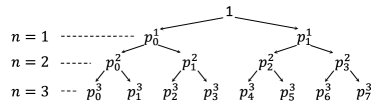
Let $x_{R}=(x_{0},\dots,x_{N-1})^{\rm T}\in{\mathbb{R}}^{N}$ and $|x_{R}\rangle=\sum_{i=0}^{N-1}\frac{x_{i}}{||x||}|i\rangle$. First we prepare the state $|x_{R}\rangle$, then add phase factors to obtain $|x\rangle$. Suppose the probability of each component denoted by $p^{n}_{i}=x_{i}^{2}/\|x\|^{2}$ is known and we define the marginal probability $p^{k}_{i}=\sum_{i^{\prime}=2i,2i+1}p^{k+1}_{i^{\prime}}$, $k=1,\dots,n-1$. Fig. 1 shows the case when $n=3$. For example, the first $n-1$ qubits is $|0\rangle^{\otimes{n-1}}$ with the probability $p_{0}^{n-1}=p^{n}_{0}+p^{n}_{1}$, and $p_{2}^{2}$ represents the probability in the case that the first $2$ qubits is $|10\rangle$.

Refer to caption
Figure 1: The marginal probabilities for $n=3$.

We briefly describe the idea of this algorithm, then show the quantum circuit representation. Let $|x^{k}_{R}\rangle=\sum_{i=0}^{2^{k}-1}\sqrt{p^{k}_{i}}|i\rangle$. For given $|x^{k}_{R}\rangle$, the basic idea is to obtain $|x^{k+1}_{R}\rangle$ by an iteration method until $k=n-1$, that is $|x^{n}_{R}\rangle=|x_{R}\rangle$. We use quantum phase estimation algorithm to acquire the contact between $|x^{k}_{R}\rangle$ and $|x^{k+1}_{R}\rangle$ in the iteration method. Lastly we apply a diagonal operator containing phase factors to $|x_{R}\rangle$ to prepare $|x\rangle$.

We suppose all $x_{i}\neq 0$ for convenience and remove this restriction later. The iteration procedure can be stated as follows.

Step 1. Prepare initial state $|x_{R}^{1}\rangle$.

$\displaystyle|x^{1}_{R}\rangle=R_{Y}(2\alpha^{0}_{0})|0\rangle,$

where $\alpha^{0}_{0}=\arccos\sqrt{p^{1}_{0}}$. Thus, $|x^{1}_{R}\rangle=\sqrt{p^{1}_{0}}|0\rangle+\sqrt{p^{1}_{1}}|1\rangle$.

Step 2. Prepare the state $|x_{R}^{2}\rangle$.

Step 2.1. Define a diagonal operator $U^{1}_{\alpha}={\rm diag}\{e^{\bm{i}\alpha^{1}_{0}},e^{\bm{i}\alpha^{1}_{1}}\}$, where $\alpha^{1}_{0}=\arccos\sqrt{p^{2}_{0}/p^{1}_{0}}$ and $\alpha^{1}_{1}=\arccos\sqrt{p^{2}_{2}/p^{1}_{1}}$. The eigenvectors of $U^{1}_{\alpha}$ are computational basis. Then use phase estimation algorithm to estimate $\alpha^{1}_{0}$, $\alpha^{1}_{1}$ by the input $|x_{R}^{1}\rangle$.

This procedure needs two registers. The first register contains $t$ qubits in the state $|0\rangle^{\otimes t}$ and the second register has a qubit with the state $|x_{R}^{1}\rangle$. Use phase estimation algorithm to estimate the eigenvalues of $U^{1}_{\alpha}$. The circuit is represented in Figure LABEL:fig_pea.

First suppose $\alpha^{1}_{l}/2\pi$ is represented in binary form with $t$ bits precisely as ideal case, then analyse the general case. The final ideal state in this step is
$\displaystyle|\psi_{1}\rangle=\sqrt{p^{1}_{0}}|y^{1}_{0}\rangle|0\rangle+\sqrt{p^{1}_{1}}|y^{1}_{1}\rangle|1\rangle,$
where $y^{1}_{l}\in[0,2^{t}-1]$ and $y^{1}_{l}\pi/2^{t-1}=\alpha^{1}_{l}$,$l=0,1$. Step 2.2. Introduce an ancilla qubit in the state $|0\rangle$ as the third register and apply $R_{Y}(2\alpha_{l}^{1})$. Due to $2\alpha_{l}^{1}=y_{l}^{1}\pi/2^{t-2}$, we can apply this rotation onto $|0\rangle$ conditioned on the first register. The quantum circuit is shown in Figure LABEL:fig_R_Yt-2.
The final state in this step is $\displaystyle|\psi_{2}\rangle=$ $\displaystyle\sqrt{p^{1}_{0}}|y^{1}_{0}\rangle|0\rangle(R_{Y}(2\alpha_{0}^{1})|0\rangle)+\sqrt{p^{1}_{1}}|y^{1}_{1}\rangle|1\rangle(R_{Y}(2\alpha_{1}^{1})|0\rangle),$ $\displaystyle=$ $\displaystyle\sqrt{p^{2}_{0}}|y^{1}_{0}\rangle|00\rangle+\sqrt{p^{2}_{1}}|y^{1}_{0}\rangle|01\rangle+\sqrt{p^{2}_{2}}|y^{1}_{1}\rangle|10\rangle+\sqrt{p^{2}_{3}}|y^{1}_{1}\rangle|11\rangle.$ Step 2.3. Use the uncomputation technique to erase $|y_{l}^{1}\rangle$ and get $|x^{2}_{R}\rangle$. We can apply the inverse of the phase estimate transformation in the first two registers. The circuit is represented as Figure LABEL:fig_inverpea.
Combining step 2.1,2.2 and 2.3, we get the whole quantum circuit representation (Figure II.1).
Figure 5: Quantum circuit to prepare $|x_{R}^{2}\rangle$.

Step 3. Take the step 2 as a submodule to obtain $|x_{R}\rangle$. Specifically, define a diagonal operator $U^{k}_{\alpha}={\rm diag}\{e^{\bm{i}\alpha^{k}_{0}},\dots,e^{\bm{i}\alpha^{k}_{2^{k}-1}}\}$, where $\alpha^{k}_{j}=\sqrt{p^{k+1}_{2j}/p^{k}_{j}}$. If there exists $x_{i}=0$ such that $p^{k}_{i^{\prime}}=0$, additionally define $\alpha^{k}_{i^{\prime}}=0$. Thus, the restriction $x_{i}\neq 0$ can be removed. Use phase estimation algorithm to estimate $\alpha^{k}_{j}$, $j=0,\dots,2^{k}-1$ by the input $|x^{k}_{R}\rangle$ and continue the remaining part of step 2 to get the output state $|x^{k+1}_{R}\rangle$. Repeat the step 2 until $k=n-1$, that is $|x^{i+1}_{R}\rangle=|x_{R}\rangle$.

Note that $4\alpha_{j}^{i}\in[0,2\pi]$, then we can always estimate $2\alpha_{j}^{i}\in[0,\pi]\subset[0,2\pi)$ by adjust $U_{\alpha}^{i},R_{Y}(\frac{y_{i}\pi}{2^{t-2}})$ to $U_{2\alpha}^{i},R_{Y}(\frac{y_{i}\pi}{2^{t-1}})$. If all $\alpha_{j}^{i}\neq\pi/2$, we can estimate $4\alpha_{j}^{i}$ in similar way.

Step 4. Add the phase factors to obtain $|x\rangle$. Define $U_{\theta}=diag\{e^{\bm{i}\theta_{0}},\dots,e^{\bm{i}\theta_{2^{n}-1}}\}$, then $|x\rangle=U_{\theta}|x_{R}\rangle$.

In this algorithm, it is necessary to estimate the exact values of eigenvalues in the phase estimation algorithm. In the general case that $\alpha^{k}_{j}/2\pi$ cannot be represented in binary form with $t$ bits precisely, we need to find an approximate diagonal operator $U^{i}_{\alpha^{(t)}}={\rm diag}\{e^{\bm{i}\alpha^{i(t)}_{0}},\dots,e^{\bm{i}\alpha^{i(t)}_{2^{i}-1}}\}$, where $\alpha^{i(t)}_{j}$ is the approximation of $\alpha^{i}_{j}$ and $\alpha^{i(t)}_{j}/2\pi$ is represented in binary form with $t$ bits precisely. The approximate operator affect the fidelity of $|x\rangle$ we discuss in section III.

II.2 Probabilistic quantum algorithms for state preparation

In this section, we introduce a probabilistic quantum algorithm for state preparation. The basic framework is still the phase estimation algorithm. Similarly, we limit $x_{i}\neq 0$ for convenience, and remove this restriction later. Let $\alpha_{i}=\arccos(x_{i}/\max\{|x_{i}|\})\in[0,\pi/2)$.

We give the whole process in Figure II.2. The unitary $U_{1}=diag\{e^{\bm{i}4\alpha_{0}},\dots,e^{\bm{i}4\alpha_{N-1}}\}$ and $U_{2}=diag\{e^{\bm{i}\theta_{0}},\dots,e^{\bm{i}\theta_{N-1}}\}$. The controlled $R_{Y}(y_{i}\pi/2^{t})$ gate is several $R_{Y}(\pi/2^{i})$ gates conditioned on the $i-$th qubit in the first register.

Figure 6: The whole circuit.

Step 1. Prepare the state $|x_{r}\rangle\triangleq\sum_{i=0}^{N-1}\frac{x_{i}}{||x||}|i\rangle$. This notation is for distinguishing $|x_{R}\rangle$ in the deterministic algorithm. First suppose $4\alpha_{i}/2\pi$ can be precisely represented in binary form with $t$ bits. In Figure II.2, the state $(1)$ is

$\displaystyle\frac{1}{\sqrt{2^{n}}}\sum_{i=0}^{2^{n}-1}|y^{i}\rangle|i\rangle,$

where $|y^{i}\rangle=|y_{1}^{i}\dots y_{t}^{i}\rangle$ is an estimate of $4\alpha_{i}$. Then we introduce an auxiliary qubit and the controlled $R_{Y}(y_{i}\pi/2^{t})$ gate. The meaning of this rotation operator can refer to Figure LABEL:fig_R_Yt-2. The state $(2)$ is

$\displaystyle\frac{1}{\sqrt{2^{n}}}\sum_{i=0}^{2^{n}-1}|y^{i}\rangle|i\rangle(\cos\alpha_{i}|0\rangle+\sin\alpha_{i}|1\rangle).$

Then use the uncomputation technique to erase $|y^{i}\rangle$ to obtain the state $(3)$

$\displaystyle\frac{1}{\sqrt{2^{n}}}\sum_{i=0}^{2^{n}-1}|i\rangle(\cos\alpha_{i}|0\rangle+\sin\alpha_{i}|1\rangle).$

Next measure the auxiliary qubit. With the probability $\frac{\|x\|^{2}}{2^{n}\max_{i}x_{i}^{2}}$ the measure result is the state $|0\rangle$ and get the state

$\displaystyle|x_{r}\rangle=\sum_{i=0}^{2^{n}-1}\frac{\cos\alpha_{i}}{\sqrt{\sum_{j}\cos^{2}\alpha_{j}}}|i\rangle=\sum_{i=0}^{N-1}\frac{x_{i}}{||x||}|i\rangle.$ (1)

Step 2. Prepare the state $|x\rangle$ by apply the diagonal operator $U_{2}$ to $|x_{r}\rangle$.

This algorithm is similar to the deterministic algorithm. We need to find an approximate diagonal operator denoted by $U_{1}^{(t)}$ to replace $U_{1}$. The success probability and fidelity of preparing $|x\rangle$ are put in section III.

From these two algorithms, we find that except the runtime of $U^{i}_{\alpha^{(t)}},U_{1}$ and $U_{\theta}(U_{2})$ the algorithm is efficient due to $t=\mathcal{O}(n)$, which means the key to solve this state preparation problem is to find a suitable way of decomposing the diagonal unitary operators. Detailed discussion is presented in the section II.3.

II.3 Diagonal unitary operator decomposition

In this section, we take the decomposition of $U_{1}$ as an example. The general decomposition is presented in the form of the theorem.

Suppose we have acquired the accurate values of the whole $\alpha_{i}$. Let $\beta_{i}=4\alpha_{i}\in[0,2\pi)$. We constantly divide the interval $[0,2\pi)$ uniformly and use $m$ to denote the number of divisions. We define $\mathcal{I}_{m}=\{0,\frac{\pi}{2^{m-1}},\frac{2\pi}{2^{m-1}},\cdots,2\pi-\frac{\pi}{2^{m-1}}\}\subset[0,2\pi)$ and let $\beta^{(m)}_{i}=\max_{\beta}\{\beta\leq\beta_{i},\beta\in\mathcal{I}_{m}\}$, that is the closed value to $\beta_{i}$. For example, for $m=1$ we limit the value of all the $\beta_{i}$ to 00 or $\pi$ and for $m=2$ we limit the value of $\beta_{i}$ to $0,\frac{\pi}{2},\pi$ or $\frac{3\pi}{2}$.

Define

$\displaystyle U_{\beta^{(m)}}=diag\{e^{\bm{i}\beta_{0}^{(m)}},\dots,e^{\bm{i}\beta_{2^{n}-1}^{(m)}}\},$

and use $U_{\beta^{(m)}}$ to replace the transformation $U_{1}$. Note that for all $m$ even if $x_{i}=0$, we have $\beta^{(m)}_{i}\neq 2\pi$, then the restriction about $x_{i}$ in section II.2 can be ignored.

We introduce some notations. For a quantum system with $n$ qubits, denote by $U_{i}$ the operator $U$ acting to the $i$-th qubit. Generally, let $Z^{(\pm l)}=\begin{bmatrix}1&0\\ 0&e^{\pm 2\pi\bm{i}/2^{l}}\end{bmatrix}$, $l\in{\mathbb{Z}}^{+}$, then we have $Z^{(\pm 1)}=Z$, $Z^{(2)}=S$ and $Z^{(3)}=T$. We denote by $C^{k}Z^{(l)}$ the controlled-$Z^{(l)}$ operator between the $k$ connected qubits and specifically denote by $C^{k}Z_{i_{1},\dots,i_{k}}$ the operator acting to $k$ qubits, whose ordinals are $i_{1},\dots,i_{k}$. And we write $Z^{(l)}_{i}=C^{1}Z^{(l)}_{i}$. Let $G^{(l)}$ be the group with multiplication operations generated by the set $\{I_{i},C^{k}Z^{(l)}\}$, $i=1,\dots,n$, $k=1,\dots,n$.

When the number of division $m=1$, this problem can be converted to the construction of the hypergraph states rossi2013quantum and be applied in the quantum neuron tacchino2018artificial . We explain the decomposition of $U_{\beta^{(m)}}$ in this case.

Lemma 1.

Suppose the values of all $\beta_{i}^{(1)}$ are known in order. Then for $m=1$,

$\displaystyle U_{\beta^{(1)}}\in G^{(1)}.$ (2)
Proof.

Each diagonal element of $U_{\beta^{(m)}}$ is $\pm 1$,

$\displaystyle U_{\beta^{(1)}}=\sum_{i=0}^{2^{n}-1}e^{\bm{i}\beta_{i}^{(1)}}|i\rangle\langle i|.$

We express the order $i$ in binary numbers for convenience. First, choose the orders $I_{1}^{(1)}$ such that the corresponding coefficient $e^{\bm{i}\beta_{i}^{(1)}}=-1$ and the order $i$ has only one digit $1$, that is $|i\rangle=|0\dots 01_{j_{i}}0\dots\rangle$. Apply all the local $Z_{j_{i}}$ gates to $U_{\beta^{(1)}}$ to get a new diagonal unitary matrix $U_{\beta_{1}^{(1)}}$,

$\displaystyle U_{\beta_{1}^{(1)}}=\otimes_{i\in I_{1}^{(1)}}Z_{j_{i}}\otimes I\cdot U_{\beta^{(1)}}=\sum_{i=0}^{2^{n}-1}e^{\bm{i}\beta_{1i}^{(1)}}|i\rangle\langle i|.$ (3)

We can see for $i\in I_{1}^{(1)}$, $e^{\bm{i}\beta_{1i}^{(1)}}=1$. Secondly, choose the orders $I_{2}^{(1)}$ such that the corresponding coefficient $e^{\bm{i}\beta_{1i}^{(1)}}=-1$ and the order $i$ has only $2$ digits $1$, that is $|i\rangle=|0\dots 01_{j_{1i}}0\dots 01_{j_{2i}}0\dots\rangle$. Apply all the $C^{2}Z_{j_{1i}j_{2i}}$ gates to $U_{\beta_{1}^{(1)}}$ to get

$\displaystyle U_{\beta_{2}^{(1)}}=\otimes_{i\in I_{2}^{(1)}}C^{2}Z_{j_{1i}j_{2i}}\otimes I\cdot U_{\beta_{1}^{(1)}}=\sum_{i=0}^{2^{n}-1}e^{\bm{i}\beta_{2i}^{(1)}}|i\rangle\langle i|.$ (4)

For $i\in I_{1}^{(1)}\cup I_{2}^{(1)}$, $e^{\bm{i}\beta_{2i}^{(1)}}=1$. In general, according to the first two steps, we can get the matrix $U_{\beta_{k}^{(1)}}$ in step $k$, $k=3,\dots,n$. In the final step, for $i\in I_{1}^{(1)}\cup\cdots\cup I_{n}^{(1)}$, $e^{\bm{i}\beta_{ni}^{(1)}}=1$, which means $U_{\beta_{n}^{(1)}}=I$.

$\displaystyle I=$ $\displaystyle C^{n}Z_{1\dots n}\cdots(\otimes_{i\in I_{2}^{(1)}}C^{2}Z_{j_{1i}j_{2i}}\otimes I^{\prime})\cdot(\otimes_{i\in I_{1}^{(1)}}Z_{j_{i}}\otimes I^{\prime\prime})U_{\beta^{(1)}}$
$\displaystyle\triangleq$ $\displaystyle C^{n}Z\cdots C^{1}Z\cdot U_{\beta^{(1)}}.$ (5)

Note that the inverse of $C^{k}Z$ is itself. Thus,

$\displaystyle U_{\beta^{(1)}}=C^{1}Z\cdots C^{n}Z.$ (6)

From Lemma 1, we know that the runtime of general decompositions of $U_{\beta^{(1)}}$ for the state preparation problems is exponential even if $m=1$. Further when the classical data is the binary strings set, this amplitude encoding method is still not efficient.

Our goal is to generalize this method for any $m$. Note that $G^{(l)}\subset G^{(l+1)}$. For any $m\geq 2$, we apply some unitary transformations $C^{k}Z^{(m)}\in G^{(m)}$ to $U_{\beta^{(m)}}$ and obtain a matrix denoted by $U_{\beta^{(m-1)}}\in G^{(m-1)}$. Repeat this procedure to get the decomposition of $U_{\beta^{(m)}}$.

Theorem 1.

Suppose the values of all $\beta_{i}^{(m)}$ are known in order, then

$\displaystyle U_{\beta^{(m)}}\in G^{(m)}.$ (7)
Proof.

Due to $\beta_{i}^{(m)}\in\mathcal{I}_{m}$, each diagonal element of $U_{\beta^{(m)}}$ is $e^{\bm{i}\beta_{i}^{(m)}}=e^{\bm{i}\frac{p_{i}\pi}{2^{m-1}}},p_{i}=0,\dots,2^{m}-1$. In the first step, choose the orders $I_{1}^{(m)}$ such that the corresponding coefficient $e^{\bm{i}\beta_{i}^{(m)}}\notin\mathcal{I}_{m-1}$ and the order $i$ has only one digit $1$, that is $|i\rangle=|0\dots 01_{j_{i}}0\dots\rangle$. Apply all the local $Z^{(m)}_{j_{i}}$ gates to $U_{\beta^{(m)}}$ to get a new diagonal unitary matrix $U_{\beta_{1}^{(m)}}$,

$\displaystyle U_{\beta_{1}^{(m)}}=\otimes_{i\in I_{1}^{(m)}}Z^{(m)}_{j_{i}}\otimes I\cdot U_{\beta^{(m)}}=\sum_{i=0}^{2^{n}-1}e^{\bm{i}\beta_{1i}^{(m)}}|i\rangle\langle i|.$ (8)

For $i\in I_{1}^{(m)}$, $\beta_{1i}^{(m)}\in\mathcal{I}_{m-1}$. Secondly, choose the orders $I_{2}^{(m)}$ such that the corresponding coefficient $e^{\bm{i}\beta_{1i}^{(m)}}\notin\mathcal{I}_{m-1}$ and the order $i$ has only $2$ digits $1$, that is $|i\rangle=|0\dots 01_{j_{1i}}0\dots 01_{j_{2i}}0\dots\rangle$. Apply all the $C^{2}Z^{(m)}_{j_{1i}j_{2i}}$ gates to $U_{\beta_{1}^{(m)}}$ to get

$\displaystyle U_{\beta_{2}^{(m)}}=\otimes_{i\in I_{2}^{(m)}}C^{2}Z^{(m)}_{j_{1i}j_{2i}}\otimes I\cdot U_{\beta_{1}^{(m)}}=\sum_{i=0}^{2^{n}-1}e^{\bm{i}\beta_{2i}^{(m)}}|i\rangle\langle i|.$ (9)

For $i\in I_{1}^{(m)}\cup I_{2}^{(m)}$, $\beta_{2i}^{(m)}\in\mathcal{I}_{m-1}$. In general, similar to the first two steps, we can get the matrix $U_{\beta_{k}^{(m)}}$ in step $k$, $k=3,\dots,n$. In the final step, for $i\in I_{1}^{(m)}\cup\cdots\cup I_{n}^{(m)}$, we have $e^{\bm{i}\beta_{ni}^{(m)}}\in\mathcal{I}_{m-1}$, which means $U_{\beta_{n}^{(m)}}\in G^{(m-1)}$.

$\displaystyle U_{\beta_{n}^{(m)}}$
$\displaystyle=$ $\displaystyle C^{n}Z^{(m)}_{1\dots n}\cdots(\otimes_{i\in I_{2}^{(m)}}C^{2}Z^{(m)}_{j_{1i}j_{2i}}\otimes I^{\prime})\cdot(\otimes_{i\in I_{1}^{(m)}}Z^{(m)}_{j_{i}}\otimes I^{\prime\prime})U_{\beta^{(m)}}$
$\displaystyle\triangleq$ $\displaystyle C^{n}Z^{(m)}\cdots C^{1}Z^{(m)}\cdot U_{\beta^{(m)}}.$ (10)

Note that the inverse of $C^{k}Z^{(m)}$ is $C^{k}Z^{(-m)}$. Thus,

$\displaystyle U_{\beta^{(m)}}=C^{1}Z^{(-m)}\cdots C^{n}Z^{(-m)}\cdot U_{\beta_{n}^{(m)}}.$ (11)

Continue this process for $U_{\beta_{n}^{(m)}}$ until the case where $m=1$, then we have

$\displaystyle U_{\beta^{(m)}}=(C^{1}Z^{(-m)}\cdots C^{n}Z^{(-m)})\cdots(C^{1}Z^{(-1)}\cdots C^{n}Z^{(-1)}).$ (12)

The Theorem 1 shows that in general the gate complexity of $U_{\beta^{(m)}}$is $\mathcal{O}(mN)$. In the section III, for the given error $\epsilon$ of the final state, the number of divisions $m(t,t\prime)$ can be regarded as $\mathcal{O}(n)$. And in particular when the classical data set $X=\{x^{i}\}\subset{\mathbb{R}}^{N}({\mathbb{C}}^{N})$ is $\mathcal{O}(n)$-sparse, that is for all $x^{i}$ the number of the nonzero components is $\mathcal{O}(n)$, the gate complexity of the diagonal unitary operator $U_{\beta^{(m)}}$ is $\mathcal{O}(n^{2})$.

III Discussions

The idea for both two algorithms is first to prepare $|x_{R}\rangle(|x_{r}\rangle)$, then add the phase factors. We discuss the fidelity for $|x_{R}\rangle$ and the fidelity and success probability for $|x_{r}\rangle$. The approximate decomposition of phase unitary transformation $U_{\theta}(U_{2})$ only affect the fidelity of preparing $|x\rangle$ from $|x_{R}\rangle(|x_{r}\rangle)$.

III.1 The fidelity for $|x_{R}\rangle$

Since the $t$ qubits in the first register can be reused, we use $U^{i}_{\alpha^{(t)}}$ to replace $U^{i}_{\alpha}$ in all the iterative process. In this section, the relationship between $t$ and the fidelity of $|x_{R}\rangle$ is expounded. For convenience, we denote the approximate vectors, angles $|x^{(t)}\rangle$, $\alpha^{(t)}$ by $|\tilde{x}\rangle$, $\tilde{\alpha}$.

Theorem 2.

For the deterministic algorithm, denote by $|\tilde{x}_{R}^{k}\rangle=\sum_{i=0}^{2^{k}-1}\sqrt{\tilde{p}_{i}^{k}}|i\rangle$ the final state in the $(k-1)$-th iterative process. If we choose $t=\lceil\log_{2}\frac{(n-1)\sqrt{2}\pi}{\epsilon}\rceil+1$, then the fidelity for $|x_{R}\rangle$ obeys the bound

$\displaystyle||{x}_{R}\rangle-|\tilde{x}_{R}^{n}\rangle|\leq\epsilon.$
Proof.

First, we discuss the error in $|x_{R}^{2}\rangle$. Define $U^{1}_{\alpha^{(t)}}={\rm diag}\{e^{\bm{i}\tilde{\alpha}^{1}_{0}},e^{\bm{i}\tilde{\alpha}^{1}_{1}}\}$, where $\tilde{\alpha}^{1}_{l}$ is the approximation of $\alpha^{1}_{l}$ such that

$\displaystyle|y_{l}^{1}-2^{t}\arccos{\sqrt{p_{2l}^{2}/p_{l}^{1}}/2\pi}|\leq 1,$

where $y_{l}^{1}=2^{t}\tilde{\alpha}^{1}_{l}/2\pi\in[0,2^{t}-1]\cap{\mathbb{Z}}$, $l=0,1$. Then we have $|\tilde{\alpha}_{l}^{1}-\arccos\sqrt{p_{2l}^{2}/p_{2l}^{1}}|\leq\pi/2^{t-1}$. Thus,

$\displaystyle||x_{R}^{2}\rangle-|\tilde{x}_{R}^{2}\rangle|\leq\sqrt{2}\pi/2^{t-1}.$

Perform the $(k-1)$-th iteration from $|\tilde{x}_{R}^{k-1}\rangle$ to prepare $|\tilde{x}_{R}^{k}\rangle$. Let $|{x^{\prime}}_{R}^{k}\rangle=\sum_{i=0}^{2^{k}-1}\sqrt{{p^{\prime}}_{i}^{k}}|i\rangle$ such that $\tilde{p}^{k-1}_{i}=\sum_{i^{\prime}=2i,2i+1}{p^{\prime}}_{i^{\prime}}^{k}$ and ${p^{\prime}}_{2i}^{k}/{p^{\prime}}_{2i+1}^{k}={p}_{2i}^{k}/{p}_{2i+1}^{k}$. Then

$\displaystyle||{x^{\prime}}_{R}^{k}\rangle-|\tilde{x}_{R}^{k}\rangle|\leq\sqrt{2}\pi/2^{t-1}.$

and

$\displaystyle||{x}_{R}^{k}\rangle-|{x^{\prime}}_{R}^{k}\rangle|=||x_{R}^{k-1}\rangle-|\tilde{x}_{R}^{k-1}\rangle|\leq(k-2)\sqrt{2}\pi/2^{t-1}.$

Thus,

$\displaystyle||{x}_{R}\rangle-|\tilde{x}_{R}^{n}\rangle|\leq(n-1)\sqrt{2}\pi/2^{t-1}.$

III.2 The fidelity and success probability for $|x_{r}\rangle$

Theorem 3.

For the probabilistic algorithm, set $t=2n+\lceil\log_{2}\frac{\pi}{\epsilon}\rceil$, then with success probability greater than $\frac{\|x\|^{2}}{2^{n}\max_{i}x_{i}^{2}}$ the fidelity for $|x_{r}\rangle$ obeys the bound

$\displaystyle||{x}_{r}\rangle-|\tilde{x}_{r}\rangle|\leq\epsilon.$
Proof.

Since $\tilde{\alpha}_{i}\leq\alpha_{i}$, the probability to measure $|0\rangle$ is

$\displaystyle\frac{\sum_{i=0}^{2^{n}-1}\cos^{2}\tilde{\alpha}_{i}}{2^{n}}\geq\frac{\sum_{i=0}^{2^{n}-1}\cos^{2}\alpha_{i}}{2^{n}}=\frac{\|x\|^{2}}{2^{n}\max_{i}x_{i}^{2}}.$

We get

$\displaystyle|\tilde{x}_{r}\rangle=\sum_{i=0}^{2^{n}-1}\frac{\cos\tilde{\alpha}_{i}}{\sqrt{\sum_{j}\cos^{2}\tilde{\alpha}_{j}}}|i\rangle.$

By (1), we have

$\displaystyle||x_{r}\rangle-|\tilde{x}_{r}\rangle|\leq$ $\displaystyle\sum_{i=0}^{2^{n}-1}\left|\frac{\cos\alpha_{i}}{\sqrt{\sum_{j}\cos^{2}\alpha_{j}}}-\frac{\cos\tilde{\alpha}_{i}}{\sqrt{\sum_{j}\cos^{2}\tilde{\alpha}_{j}}}\right|$
$\displaystyle\leq$ $\displaystyle\sum_{i=0}^{2^{n}-1}\left|\frac{\cos\alpha_{i}}{\sqrt{\sum_{j}\cos^{2}\alpha_{j}}}-\frac{\cos\tilde{\alpha}_{i}}{\sqrt{\sum_{j}\cos^{2}\alpha_{j}}}\right|$
$\displaystyle+\sum_{i=0}^{2^{n}-1}\left|\frac{\cos\tilde{\alpha}_{i}}{\sqrt{\sum_{j}\cos^{2}\alpha_{j}}}-\frac{\cos\tilde{\alpha}_{i}}{\sqrt{\sum_{j}\cos^{2}\tilde{\alpha}_{j}}}\right|.$

Since $|\alpha_{i}-\tilde{\alpha}_{i}|<\pi/2^{t+1}\triangleq\delta$, we have

$\displaystyle|\cos\alpha_{i}-\cos\tilde{\alpha}_{i}|<\delta.$ (13)

Note that $|x_{r}\rangle\neq 0$, which means $\sum_{i}\cos^{2}\alpha_{j}\geq 1$ and we have

$\displaystyle\left|\frac{1}{\sqrt{\sum_{j}\cos^{2}\alpha_{j}}}-\frac{1}{\sqrt{\sum_{j}\cos^{2}\tilde{\alpha}_{j}}}\right|\leq 2^{n}\delta.$ (14)

Combining expressions (13)(14), we obtain

$\displaystyle||x_{r}\rangle-|\tilde{x}_{r}\rangle|\leq 2^{2n+1}\frac{\pi}{2^{t+1}}.$

Let $t=2n+\lceil\log_{2}\frac{\pi}{\epsilon}\rceil$, we have $||{x}_{r}\rangle-|\tilde{x}_{r}\rangle|\leq\epsilon$.

III.3 The fidelity and success probability for $|x\rangle$

Suppose $|x_{R}\rangle(|x_{r}\rangle)$ is prepared precisely. By Setting $U_{\theta^{(t^{\prime})}}$ to replace $U_{\theta}(U_{2})$, we have $||x\rangle-|x^{(t^{\prime})}\rangle|\leq 2^{n}\pi/2^{t^{\prime}-1}$. Let $\epsilon^{\prime}=\epsilon/2$, then we obtain $|x\rangle-|x^{(t^{\prime})}\rangle|\leq\epsilon^{\prime}$ when setting $t^{\prime}=n+1+\lceil\log_{2}\frac{\pi}{\epsilon^{\prime}}\rceil$. Combine Theorem 2 and Theorem 3, then we have the result

Theorem 4.

For the deterministic algorithm, set $t=\lceil\log_{2}\frac{2(n-1)\sqrt{2}\pi}{\epsilon}\rceil+1$, $t^{\prime}=n+1+\lceil\log_{2}\frac{2\pi}{\epsilon}\rceil$, then the fidelity for $|x\rangle$ obeys the bound

$\displaystyle||x\rangle-|\tilde{x}\rangle|\leq\epsilon.$
Theorem 5.

For the probabilistic algorithm, set $t=2n+\lceil\log_{2}\frac{2\pi}{\epsilon}\rceil$, $t^{\prime}=n+1+\lceil\log_{2}\frac{2\pi}{\epsilon}\rceil$, then with success probability greater than $\frac{\|x\|^{2}}{2^{n}\max_{i}x_{i}^{2}}$ the fidelity for $|x\rangle$ obeys the bound

$\displaystyle||x\rangle-|\tilde{x}\rangle|\leq\epsilon.$

IV Conclusion

We introduce two algorithms of amplitude encoding for state preparation problems. In this method, for a vector $x\in{\mathbb{C}}^{N}$ we need $\log_{2}N$ qubits to construct the corresponding quantum state $|x\rangle$ with exponential depth. We analyse the fidelity for the deterministic algorithm and the probabilistic algorithm and discuss the success probability in the probabilistic algorithm. This success probability is decided by the data structure.

We turn the state preparation problem to the decomposition problem of the diagonal unitary operators. The runtime in these algorithms whose corresponding circuits are limited to the width $\mathcal{O}(n)$ is exponential to $n$ generally. However, in certain cases, the decomposition of diagonal unitary transformations naturally only contains polynomial layers; e.g., the classical data set is $O(n)$-sparse. In other words, the quantum states whose corresponding diagonal unitary operators have polynomial decompositions can be prepared effectively.

acknowledgements

This work was supported by the National Key Research and Development Program of China (Grant No. 2016YFA0301700) and the Anhui Initiative in Quantum Information Technologies (Grant No. AHY080000).

References

  • [1] Jacob Biamonte, Peter Wittek, Nicola Pancotti, Patrick Rebentrost, Nathan Wiebe, and Seth Lloyd. Quantum machine learning. Nature, 549(7671):195, 2017.
  • [2] Maria Schuld and Francesco Petruccione. Supervised Learning with Quantum Computers, volume 17. Springer, 2018.
  • [3] Seth Lloyd, Masoud Mohseni, and Patrick Rebentrost. Quantum principal component analysis. Nature Physics, 10(9):631, 2014.
  • [4] Aram W Harrow, Avinatan Hassidim, and Seth Lloyd. Quantum algorithm for linear systems of equations. Physical review letters, 103(15):150502, 2009.
  • [5] Dan Ventura and Tony Martinez. Quantum associative memory. Information Sciences, 124(1-4):273–296, 2000.
  • [6] Christophe Andrieu, Nando De Freitas, Arnaud Doucet, and Michael I Jordan. An introduction to mcmc for machine learning. Machine learning, 50(1-2):5–43, 2003.
  • [7] Seth Lloyd. Universal quantum simulators. Science, pages 1073–1078, 1996.
  • [8] Iulia M Georgescu, Sahel Ashhab, and Franco Nori. Quantum simulation. Reviews of Modern Physics, 86(1):153, 2014.
  • [9] Lov Grover and Terry Rudolph. Creating superpositions that correspond to efficiently integrable probability distributions. arXiv preprint quant-ph/0208112, 2002.
  • [10] Phillip Kaye and Michele Mosca. Quantum networks for generating arbitrary quantum states. arXiv preprint quant-ph/0407102, 2004.
  • [11] Mikko Mottonen, Juha J Vartiainen, Ville Bergholm, and Martti M Salomaa. Transformation of quantum states using uniformly controlled rotations. arXiv preprint quant-ph/0407010, 2004.
  • [12] Andrei N Soklakov and Rüdiger Schack. Efficient state preparation for a register of quantum bits. Physical Review A, 73(1):012307, 2006.
  • [13] Vittorio Giovannetti, Seth Lloyd, and Lorenzo Maccone. Quantum random access memory. Physical review letters, 100(16):160501, 2008.
  • [14] John A Cortese and Timothy M Braje. Loading classical data into a quantum computer. arXiv preprint arXiv:1803.01958, 2018.
  • [15] Michael A Nielsen and Isaac Chuang. Quantum computation and quantum information, 2002.
  • [16] Matteo Rossi, M Huber, D Bruß, and C Macchiavello. Quantum hypergraph states. New Journal of Physics, 15(11):113022, 2013.
  • [17] Francesco Tacchino, Chiara Macchiavello, Dario Gerace, and Daniele Bajoni. An artificial neuron implemented on an actual quantum processor. arXiv preprint arXiv:1811.02266, 2018.