Optimal ratchet current for elastically interacting particles

Abstract

In this work we show that optimal ratchet currents of two interacting particles are obtained when stable periodic motion is present. By increasing the coupling strength between identical ratchet maps, it is possible to find, for some parametric combinations, current reversals, hyperchaos, multistability, and duplication of the periodic motion in the parameter space. Besides that, setting a fixed value for the current of one ratchet it is possible to induce a positive/negative/null current for the whole system in certain domains of the parameter space.

Ratchet models are well-known prominent candidates to describe the transport phenomenon in nature in the absence of external bias. The ratchet effect is defined as the rectification of an external net-zero force to obtain a directional transport of particles in spatially periodic media. While single ratchet systems have been extensively studied in the literature, the dynamics in coupled ratchets is almost unknown. In this work we exhaustively explore the parameter space of two elastically coupled ratchet model and characterize the global dynamics of the whole system for a symmetric coupling configuration. The parameters of the system are the coupling strength of elastic interaction between the ratchets, the damping factor, and the ratchet potential amplitude. Such simple configuration is enough to produce competing influences between the ratchets and leads to the appearance of complex behaviors as hyperchaotic dynamics, current reversals and multistability observed in phase and parameter spaces.

I Introduction

Ratchets are physical devices constructed in such a clever way that they are able to transport particles with nonzero macroscopic velocity in the absence of macroscopic external bias. They only operate with success when time and spatial symmetries are simultaneously broken. The motion of single Brownian particles in ratchet-like devices has attracted great attention in the last decades due to its great ability to describe systems and phenomena as molecular motors Zhou and Chen (1996); Reimann (2002); Astumian (1997), coupled Josephson junctions Zapata et al. (1996), mass separation Kettner et al. (2000) and transport of solitons in crystals Brox et al. (2017), among many others. In the context of molecular motors (protein molecules that perform essential tasks to the life of the organism like muscle contraction, intracellular transport, and cell division), the ratchet model has helped to understand how they operate Astumian and Hänggi (2002). A crucial advance in the understanding of how optimal ratchets currents are generated was only obtained when the relation between optimal ratchet currents (RCs) and the Isoperiodic Stable Structures (ISSs) was established Celestino et al. (2011). The ISSs, observed in many dissipative continuous- and discrete-time dynamical systems Fraser and Kapral (1982); Carcasses et al. (1991); Gallas (1993); Bonatto et al. (2005); Bonatto and Gallas (2007); Stoop et al. (2010); da Costa et al. (2016), delimit the range of available parameters which lead to regular orbits. Most importantly, the ISSs appear along preferred directions in the parameter space furnishing a guide to follow the optimal ratchet current Celestino et al. (2011).

The relevance of parameters chosen inside ISSs for the generation of optimal currents in coupled ratchet devices is completely unknown. The main goal of the present work is to characterize this relevance. Realistic systems are composed of many interacting particles and it is not clear what is the contribution of the mutual particle interaction on the ratchet current. Thus, in this work we start showing the effects of the elastic interaction between two ratchet devices on the current inside ISSs. Some transport properties of an elastically coupled lattice of particles in a periodically flashing ratchet potential has already been examined Chen et al. (2005). They demonstrated that mutual couplings among particles may improve the transport efficiency when the coupling strength overcomes a threshold and the interaction between the particles clearly influences the directed motion. An effective potential for the center-of-mass of particles has been proposed Wang and Bao (2004) in order to understand this behaviour.

This paper is organized as follows. Section II presents the model of coupled maps, summarizes some properties of the uncoupled ratchet map and defines the ratchet current. Discussions and results are given in Sec. III for two identical coupled ratchet maps, and in Sec. IV for distinct coupled ratchet maps. Finally in Sec. V we present the conclusions.

II Two coupled-ratchets model

The model studied in this work is composed of two-coupled Ratchet Maps (RMs) Wang et al. (2007); Celestino et al. (2011) which may present distinct dynamical properties. The coupling force between the ratchets is elastic Vincent et al. (2010); Levien and Bressloff (2015) according to:

$$\mbox{\bf RM}^{(1)}\left\{\begin{array}[]{llll}p^{\prime}_{1}=&\gamma_{1}p_{1}+K_{1}[\sin(x_{1})+a\hskip 1.42271pt\sin(2x_{1}+\phi)]\\ &+\,c\,(x_{2}-x_{1}),\\ x^{\prime}_{1}=&x_{1}+p^{\prime}_{1},\\ \end{array}\right.$$ (1)

$$\mbox{\bf RM}^{(2)}\left\{\begin{array}[]{llll}p^{\prime}_{2}=&\gamma_{2}p_{2}+K_{2}[\sin(x_{2})+a\hskip 1.42271pt\sin(2x_{2}+\phi)]\\ &+\,c\,(x_{1}-x_{2}),\\ x^{\prime}_{2}=&x_{2}+p^{\prime}_{2},\\ \end{array}\right.$$

where $K_{i}$, for $i=1,2$, are the nonlinearity parameters and $c$ is the coupling constant. The prime represents the discrete time evolution. This model describes the dynamics of two coupled particles that move on the $x$ direction with $x\in(-\infty,+\infty)$ in a asymmetric potential, while $p$ is the conjugate momentum of $x$ and $\gamma_{i}\in[0,1]$ represents the dissipation of particle $i$. The spatial symmetry is broken when $a\neq 0$ and $\phi\neq l\pi$, where $l$ is an integer. In the present work we kept fixed the parameters $a=0.5$ and $\phi=\pi/2$ Celestino et al. (2011); da Silva et al. (2018a) and studied the two dimensional parameter space $(K_{2},\gamma_{2})$ for the map $\mbox{\bf RM}^{(2)}$ using different parametric combinations $(K_{1},\gamma_{1})$ for the map $\mbox{\bf RM}^{(1)}$ setting different intensities for $c$. In Section III the case $(K_{1},\gamma_{1})=(K_{2},\gamma_{2})$ was analysed and in Section IV the parameter combination $(K_{1},\gamma_{1})$ was kept fixed, allowing to choose the momentum of the particle $i=1$.

The quantity that gives us insights about transport properties of the $i$-th RM is the Ratchet Current (RC) $\mathcal{J}_{i}$, defined as a double average of the momentum $p_{i}$:

$$\mathcal{J}_{i}=\dfrac{1}{M}\displaystyle\sum_{k=1}^{M}\left[\dfrac{1}{N}\displaystyle\sum_{n=1}^{N}p_{i}^{(k,n)}\right],$$ (2)

where $M$ is the number of initial conditions (ICs) and $N$ the total iteration time. The ICs must be equally distributed between the interval $(x_{i}^{\mbox{\tiny min}},x_{i}^{\mbox{\tiny max}})=(p_{i}^{\mbox{\tiny min}},p_{i}^{\mbox{\tiny max}})=(-2\pi,2\pi)$, since they can not establish an preferred direction. For the system (1), the total ratchet current (TRC) $\mathcal{J}_{T}$ is give by

$$\mathcal{J}_{T}=\mathcal{J}_{1}+\mathcal{J}_{2}.$$ (3)

By this definition, the TRC tends to zero when $p_{1}=-p_{2}$, while the maximum magnitude for TRC is obtained when $p_{1}$ and $p_{2}$ have the same direction and assume the maximum value.

III Coupling of two identical RMs

To determine the influence of the coupling strength $c$ on the dynamics of the system (1), we start plotting the parameter space $(K_{2},\gamma_{2})$ with colors representing the respective TRC $\mathcal{J}_{T}$ (see color bars in the figures). The first case considered, shown in Fig. 1, consists of a system of two identical coupled RMs for which $(K_{1},\gamma_{1})=(K_{2},\gamma_{2})$. Figure 1(a) shows $\mathcal{J}_{T}$ for the uncoupled case $c=0$. The configuration observed in the parameter space is identical to that obtained for a single map (see e.g. Refs. Celestino et al. (2011); da Silva et al. (2018a)). The difference is that the colors in Fig. 1 represent the TRC for the system (1). In the uncoupled case $\mathcal{J}_{T}=2\mathcal{J}_{1}=2\mathcal{J}_{2}$, since the maps are equal. As can be seen in the palette positioned to the right of Fig. 1, black color represents TRCs close to zero, increasing positive TRCs are found in regions with colors going from cyan to blue, and increasing negative TRCs are identified by the colors changing from yellow to red.    

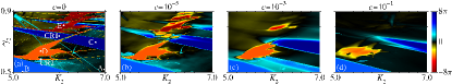
Figure 1: (Color online) Parameter space $(K_{2},\gamma_{2})$ with colors representing the TRC $\mathcal{J}_{T}$ for the system (1) in (a) ($c=0$), (b) ($c=10^{-5}$), (c) ($c=10^{-3}$), and (d) ($c=10^{-1}$), considering the coupling of two identical RMs [$(K_{1},\gamma_{1})=(K_{2},\gamma_{2})$]. For each parametric combination $(K_{2},\gamma_{2})$, $\mathcal{J}_{T}$ was obtained using $10^{4}$ ICs and $N=5\times 10^{4}$ iterations after a transient time of $8\times 10^{4}$ iterations.

It is well established in the literature that, for the uncoupled case, most regions with zero RCs correspond to a chaotic dynamics, while parametric combinations that lead to optimized values of RCs are delimited by the ISSs Celestino et al. (2011).

Increasing the coupling strength $c$, it is possible to note in Figs. 1(b), 1(c), and 1(d) that the coupling tends to destroy the ISSs, starting from their antennas, decreasing the amount of parametric combinations that generates non-zero RCs. Such destruction of the ISSs is similar to what is observed in ratchet subjected to noise or temperature (for more details see Manchein et al. (2013); Horstmann et al. (2017); da Silva et al. (2018a)). Besides that, it is possible to observe a small translation in parameter space from those ISSs which resist to larger coupling strengths and contain positive or negative TRCs.

III.1 Current Reversal

In the system composed of two identical RMs we can observe that, increasing the coupling intensity $c$, the direction of particle’s motion changes in some regions of the parameter space. To demonstrate this phenomenon (also exhibited in continuous-time dynamical systems of two interacting ratchets Vincent et al. (2010); Li et al. (2016)), we highlighted two parametric combinations: ($i$) $(K_{1},\gamma_{1})=(K_{2},\gamma_{2})=(6.0,0.74)$, indicated in Fig. 1(a) by the white point CR1; and ($ii$) $(K_{1},\gamma_{1})=(K_{2},\gamma_{2})=(5.6,0.585)$, indicated in Fig. 1(a) by the white point CR2. To analyze the current reversal, we kept fixed these parametric combinations and increased slightly the coupling strength $c$. For each value of $c$, we performed the calculation of $\mathcal{J}_{T}$ using $10^{4}$ ICs equally distributed between the interval $(x_{i}^{\mbox{\tiny min}},x_{i}^{\mbox{\tiny max}})=(p_{i}^{\mbox{\tiny min}},p_{i}^{\mbox{\tiny max}})=(-2\pi,2\pi)$ and $N=5\times 10^{4}$ iterations after a transient time of $8\times 10^{4}$ iterations.

In Fig. 2(a) the behavior of $\mathcal{J}_{T}$ as a function of $c$ for the case ($i$) is plotted. For this parametric combination, $\mathcal{J}_{T}\approx 8\pi$ for $c=0$, since we have the sum of two uncoupled particles with RC $\mathcal{J}_{i}\approx 4\pi$. The current reversal from $\mathcal{J}_{T}>0$ to $\mathcal{J}_{T}<0$ occurs for $c\approx 3\times 10^{-6}$. The negative TRC with maximum magnitude is obtained for $c\approx 2.9\times 10^{-5}$, and is $\mathcal{J}_{T}\approx-10.745215$. For this case, increasing the value of $c$, the TRC tends to zero. In Fig. 2(b) the same analysis is shown but for the case ($ii$), for which we have a transition from $\mathcal{J}_{T}<0$ to $\mathcal{J}_{T}>0$ that occurs for $c\approx 2.4\times 10^{-4}$. For this parametric combination, $\mathcal{J}_{T}\approx-4\pi$ if $c=0$ and for $c>2.4\times 10^{-4}$ the value of TRC stabilizes around $+\pi$. Additional simulations (not shown here) demonstrate that the TRC remains around $+\pi$ until $c\approx 10^{-2}$ and, after this coupling strength, $\mathcal{J}_{T}$ tends to zero.

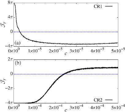
Figure 2: (Color online) TRC $\mathcal{J}_{T}$ as a function of $c$ for the system (1) considering the coupling of two identical RMs with $(K_{1},\gamma_{1})=(K_{2},\gamma_{2})=(6.0,0.74)$ in (a) [white point CR1 in Fig. 1(a)] and $(K_{1},\gamma_{1})=(K_{2},\gamma_{2})=(5.6,0.585)$ in (b) [white point CR2 in Fig. 1(a)]. For each value of $c$, $\mathcal{J}_{T}$ was obtained using $10^{4}$ ICs and $N=5\times 10^{4}$ iterations after a transient time of $8\times 10^{4}$ iterations.

III.2 Duplication of ISSs

Using strong coupling intensities in the system (1) we can observe that the domain of the parameter space with negative RCs is duplicated, as shown in Fig. 1(d) for $c=10^{-1}$. Recently, similar findings were reported in time discrete dynamical systems by using external periodic perturbations to generate multiple attractors in phase space and ISSs in the parameter space Manchein et al. (2017); da Silva et al. (2017). Increasing the intensity of the external perturbation, the regular structures start to separate from each other and an effective enlargement of the available stable domain in the parameter space is obtained. This methodology was successfully applied in the RM to retain thermal effects and to increase the area of the parameter space that leads to optimal RCs da Silva et al. (2018a). In the case of continuous systems, new stable attractors are not created but the steering of the existing multiple attractors in phase space was used to increase the regular region of the parameter space for the Langevin equation and for the Chua’s electronic circuit da Silva et al. (2018b). This results lead us to conclude that duplications of stable regimes are closely related to multistability.

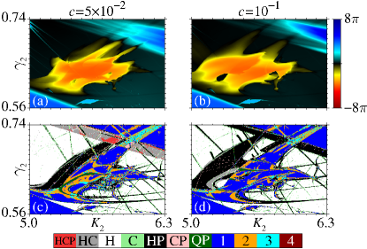
Figure 3: (Color online) Parameter space $(K_{2},\gamma_{2})$ with colors representing the TRC $\mathcal{J}_{T}$ for the system (1) in (a) ($c=5\times 10^{-2}$) and (b) ($c=10^{-1}$), and the different classes of attractors found in each parametric combination in (c) ($c=5\times 10^{-2}$) and (d) ($c=10^{-1}$).

To investigate the process behind the duplication in the case of the coupled system (1), we focus on the parametric range presented in Fig. 3 for couplings $c=5\times 10^{-2}$ and $c=1\times 10^{-1}$. We can observe in Figs. 3(a) and 3(b) (see color bar) that increasing the value of $c$ a second parametric domain with negative RC (yellow and red) arises and these two identical regions start to move away from each other. In Figs. 3(c) and 3(d) the same range was analyzed, but the colors now represent the possible combinations of different classes of attractors that can be found for the same point $(K_{1},\gamma_{1})=(K_{2},\gamma_{2})$ in the parameter space. To obtain this information, we use $81$ ICs for each parametric combination and look at the values of the Lyapunov exponents (LEs) of the resulting trajectories. For a periodic attractor (P), $\lambda_{i}<0$ for $i=1,2,3,4$. A chaotic attractor (C) takes place if $\lambda_{1}>0$ and $\lambda_{i}<0$, for $i=2,3,4$, while a hyperchaotic attractor (H) is typically defined as a chaotic attractor with at least two positive Lyapunov exponents. In addition to these three, there is another type of dynamical motion that is common: the quasiperiodic motion. A bounded orbit that is not asymptotically periodic and that does not exhibit sensitive dependence on initial conditions is called quasiperiodic Alligood et al. (1996). Thus, for a quasiperiodic attractor (QP) we have $\lambda_{1}=0$ and $\lambda_{i}<0$ for $i=2,3,4$, or $\lambda_{1}=\lambda_{2}=0$ and $\lambda_{i}<0$ for $i=3,4$. Given the above definitions, in Figs. 3(c) and 3(d) it is possible to find, for the same point in the parameter space, the following classes of attractors:

• HCP: hyperchaotic, chaotic, and periodic attractors;

• HC: hyperchaotic and chaotic attractors;

• H: only hyperchaotic attractors;

• C: only chaotic attractors;

• HP: hyperchaotic and periodic attractors;

• CP: chaotic and periodic attractors;

• QP: quasiperiodic and periodic attractors;

• 1, 2, 3, and 4 different periodic attractors.

Some of these combinations of coexisting attractors can be seen in Fig. 4, that shows the projection of the phase space $(x_{1},p_{1},x_{2},p_{2})$ of the system (1) in the plane $(x_{2},p_{2})$, considering the coupling strength $c=5\times 10^{-2}$.

In Fig. 4(a) the hyperchaotic (blue), the chaotic (yellow) and the periodic (black) attractors found for $(K_{1},\gamma_{1})=(K_{2},\gamma_{2})=(5.8,0.71)$ are plotted. This parametric combination is indicated in Fig. 3(c) by the red color (HCP). Figure 4(b) shows the hyperchaotic (blue) and the periodic (black) attractors that can be found for $(K_{1},\gamma_{1})=(K_{2},\gamma_{2})=(5.4,0.65)$, parametric combination indicated in Fig. 3(c) by the black color (HP). A quasiperiodic attractor (red) is plotted in Fig. 4(c) along with a periodic attractor (black), both found for $(K_{1},\gamma_{1})=(K_{2},\gamma_{2})=(5.3,0.61)$. The regions of the parameter space for which we found at least one quasiperiodic attractor are indicated in Figs. 3(c) and 3(d) by the green color (QP). These domains are located inside the ISSs, next to the parameters for which period doubling bifurcations occur for the uncoupled case. The coexistence of two periodic attractors that occurs for    

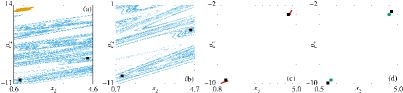
Figure 4: (Color online) Projection of the four-dimensional phase space $(x_{1},p_{1},x_{2},p_{2})$ in the plane $(x_{2},p_{2})$ showing the different classes of attractors found in (a) $(K_{1},\gamma_{1})=(K_{2},\gamma_{2})=(5.8,0.71)$: HCP - hyperchaotic (blue), chaotic (yellow) and periodic (black) attractors; (b) $(K_{1},\gamma_{1})=(K_{2},\gamma_{2})=(5.4,0.65)$: HP - hyperchaotic (blue) and periodic (black) attractors; (c) $(K_{1},\gamma_{1})=(K_{2},\gamma_{2})=(5.3,0.61)$: QP - quasiperiodic (red) and periodic (black) attractors; and (d) $(K_{1},\gamma_{1})=(K_{2},\gamma_{2})=(5.4,0.63)$: 2 different periodic attractors (black and green), all cases using $c=5\times 10^{-2}$.

$(K_{1},\gamma_{1})=(K_{2},\gamma_{2})=(5.4,0.63)$ is shown in Fig. 4(d). To identify different periodic attractors, we compared the largest LE $\lambda_{1}$ and the total time average $\langle p_{1}\rangle+\langle p_{2}\rangle$ obtained for each attractor between them. These quantities are calculated along a trajectory of $5\times 10^{6}$ iterations reached after a transient time of $1.2\times 10^{7}$ iterations. In Fig. 4(d) it is possible to note that the time average $\langle p_{1}\rangle+\langle p_{2}\rangle$ is the same for the two periodic attractors which have period $2$. However, they can be differentiated by the respective values of $\lambda_{1}$.

Figures 3(c) and 3(d) show that the duplication of the region with negative RC is due to the birth of the black region in which a hyperchaotic and a period-2 attractor coexist, scenario displayed in Fig. 4(b) for the case with $c=5\times 10^{-2}$. In this region of the parameter space, the hyperchaotic attractor [blue color in Fig. 4(b)] has time average $\langle p_{1}\rangle+\langle p_{2}\rangle\approx-2$, and for the period-2 attractor [black color in Fig. 4(b)] this value is around $-4\pi$. Since the basin of attraction of the period-2 attractor is larger ($99\%$ of the $10^{4}$ ICs used) than the basin of attraction of the hyperchaotic one, this parametric domain is characterized by a negative RC.

IV Coupling of two different RMs

The next step is to keep fixed the values $(K_{1},\gamma_{1})$ for the map $\mbox{\bf RM}^{(1)}$ and change the parameters $(K_{2},\gamma_{2})$. The values $(K_{1},\gamma_{1})$ were chosen according to the value of $\mathcal{J}_{1}$. The purpose of this study is to determine how the current of the particle $i=1$ influences the current $\mathcal{J}_{T}$ of the whole system. The parametric combinations used for this analysis are indicated in Fig. 1(a) by the white points A, B, C, D, and E, and Table 1 specifies the period of the orbit obtained and the value of $\mathcal{J}_{1}$.

Table 1: Fixed values used for $K_{1}$ and $\gamma_{1}$ in model (1) and marked as white points in Fig. 1(a).

Label	$(K_{1},\gamma_{1})$	Period	$\mathcal{J}_{1}$
A	$(7.0,0.52)$	chaos	$0.02869127$
B	$(5.2,0.50)$	$1$	$6.28318531$
C	$(6.8,0.70)$	$1$	$12.56637061$
D	$(5.6,0.64)$	$2$	$-6.28318531$
E	$(6.1,0.81)$	$2$	$-12.56637061$

IV.1 $\mbox{\bf RM}^{(1)}$ with $\mathcal{J}_{1}\sim 0$

The first case analyzed is $(K_{1},\gamma_{1})=(7.0,0.52)$, for which a chaotic dynamics is obtained for the map $\mbox{\bf RM}^{(1)}$ and the RC $\mathcal{J}_{1}$ is around zero. The parameter space $(K_{2},\gamma_{2})$ is displayed in Figs. 5(a), 5(b), and 5(c), with coupling strengths $c=10^{-7},10^{-5}$ and $c=10^{-3}$, respectively. In Fig. 5(a) it is possible to note that weak couplings between the particles have a similar effect on the ISSs as weak noise, namely to destroy only the antennas of the ISSs. The same is observed for the case $(K_{1},\gamma_{1})=(K_{2},\gamma_{2})$.

   

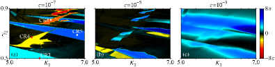
Figure 5: (Color online) Parameter space $(K_{2},\gamma_{2})$ with colors representing the TRC $\mathcal{J}_{T}$ for the system (1) using (a) $c=10^{-7}$, (b) $c=10^{-5}$, and (c) $c=10^{-3}$. The parametric combination $(K_{1},\gamma_{1})=(7.0,0.52)$ [white point A in Fig. 1(a)] was kept fixed, giving rise to a chaotic dynamics with $\mathcal{J}_{1}\approx 0$ for the map $\mbox{\bf RM}^{(1)}$, according to Table 1.

In Fig. 5(b), for which an intensity $c=10^{-5}$ was applied, unexpected current reversals can be observed. To treat this phenomenon in more detail, we indicate in Fig. 5(a) four parametric combinations $(K_{2},\gamma_{2})$ for which the current reversal occurs. They are: (1) CR3: $(K_{2},\gamma_{2})=(5.8,0.50)$; (2) CR4: $(K_{2},\gamma_{2})=(5.6,0.67)$; (3) CR5: $(K_{2},\gamma_{2})=(6.8,0.69)$; and (4) CR6: $(K_{2},\gamma_{2})=(6.1,0.81)$. The value of the TRC $\mathcal{J}_{T}$ as a function of $c$ for these parametric combinations is plotted in Fig. 6. This figure shows that for the points CR3 and CR5 the transition occurs from $\mathcal{J}_{T}>0$ to $\mathcal{J}_{T}<0$, while for CR4 and CR6 the transition occurs from $\mathcal{J}_{T}<0$ to $\mathcal{J}_{T}>0$. Beside this, it is possible to note that these transitions happen for weak couplings ($c\sim 10^{-6}$). Fig. 5(c) shows that no regions with negative TRCs can be found anymore when using $c=10^{-3}$.

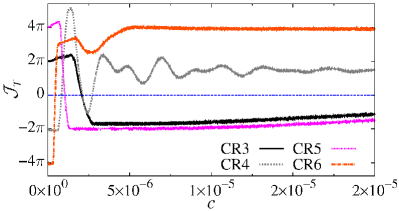
Figure 6: (Color online) TRC $\mathcal{J}_{T}$ as a function of $c$ for the system (1) considering the coupling of a chaotic map with $(K_{1},\gamma_{1})=(7.0,0.52)$ and the map $\mbox{\bf RM}^{(2)}$ with parameters $(K_{2},\gamma_{2})$ indicated by the white points CR3, CR4, CR5, and CR6 in Fig. 5(a). For each value of $c$, $\mathcal{J}_{T}$ was obtained using $10^{4}$ ICs and $N=5\times 10^{4}$ iterations after a transient time of $8\times 10^{4}$ iterations.

IV.2 $\mbox{\bf RM}^{(1)}$ with $\mathcal{J}_{1}>0$

Figure 7 shows the parameter space $(K_{2},\gamma_{2})$ of the map $\mbox{\bf RM}^{(2)}$ coupled to $\mbox{\bf RM}^{(1)}$ with parametric combinations $(K_{1},\gamma_{1})=(5.2,0.5)$ [white point B in Fig. 1(a)] and $(K_{1},\gamma_{1})=(6.8,0.7)$ [white point C in Fig. 1(a)], both cases leading to a period-1 stable attractor. For the uncoupled case plotted in Fig. 1(a), ISSs with period-1 contain positive RCs and are organized along a preferential direction. Along this direction, the absolute value of the RC increases $2\pi$ inside ISSs of same period Celestino et al. (2011). For instance, the parametric combinations indicated by the white points B and C in Fig. 1(a) have RCs $\mathcal{J}_{1}\approx 2\pi$ and $\mathcal{J}_{2}\approx 4\pi$, respectively, according to Table 1. Keeping fixed the parameter-pair $(K_{1},\gamma_{1})=(5.2,0.5)$ in model (1), the results are shown in Figs. 7(a) for $c=10^{-7}$, 7(b) for $c=10^{-5}$, and 7(c) for $c=10^{-3}$.

In Fig. 7(a) we can see that, by keeping fixed the value $\mathcal{J}_{1}\approx 2\pi$ for the map $\mbox{\bf RM}^{(1)}$, it is possible to generate a TRC $\mathcal{J}_{T}=0$ (black color) in the parametric domain inside the ISS that originally contain RC with value around $-2\pi$ in the uncoupled case. Increasing the coupling between the maps to $c=10^{-5}$ and to $c=10^{-3}$, the ISSs with negative TRC (yellow and red regions) collapse to a single region of the parameter space. For $c=10^{-3}$ [Fig. 7(c)], the positive TRCs indicated by the different shades    

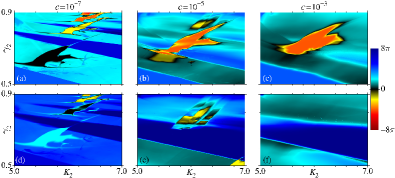
Figure 7: (Color online) Parameter space $(K_{2},\gamma_{2})$ with colors representing the TRC $\mathcal{J}_{T}$ for the system (1). In (a) ($c=10^{-7}$), (b) ($c=10^{-5}$), and (c) ($c=10^{-3}$) the parametric combination $(K_{1},\gamma_{1})=(5.2,0.5)$ [white point B in Fig. 1(a)] was kept fixed, resulting in orbits with period-1 for the map $\mbox{\bf RM}^{(1)}$ and in a RC $\mathcal{J}_{1}\approx 2\pi$, according to Table 1. In (d) ($c=10^{-7}$), (e) ($c=10^{-5}$), and (f) ($c=10^{-3}$) the parametric combination $(K_{1},\gamma_{1})=(6.8,0.7)$ [white point C in Fig. 1(a)] was kept fixed, resulting in orbits with period-1 for the map $\mbox{\bf RM}^{(1)}$ and in a RC $\mathcal{J}_{1}\approx 4\pi$, according to Table 1.

of blue occupy the most part of the parameter space $(K_{2},\gamma_{2})$. Choosing $(K_{1},\gamma_{1})=(6.8,0.7)$, for which $\mathcal{J}_{1}\approx 4\pi$, similar results are obtained. In Fig. 7(d), which shows the case $c=10^{-7}$, we can note a zero TRC $\mathcal{J}_{T}$ (black color) in the region inside the ISS that has RC around $-4\pi$ for the uncoupled case. Using $c=10^{-5}$, case plotted in Fig. 7(e), only a small parametric domain lead to negative TRCs, while using $c=10^{-3}$, case showed in Fig. 7(f), only positive TRCs can be found.

IV.3 RM⁽¹⁾ with $\mathcal{J}_{1}<0$

Now we present in Fig. 8 the results obtained by keeping fixed $(K_{1},\gamma_{1})=(5.6,0.64)$ [white point D in Fig. 1(a)] and $(K_{1},\gamma_{1})=(6.1,0.81)$ [white point E in Fig. 1(a)] for the map $\mbox{\bf RM}^{(1)}$. Considering the uncoupled case ($c=0$), the resulting RCs for these parametric combinations are $\mathcal{J}_{1}\approx-2\pi$ and $\mathcal{J}_{1}\approx-4\pi$, in this order, both cases associated with period-2 attractors (see Table 1). Figure 8(a), obtained using $(K_{1},\gamma_{1})=(5.6,0.64)$ and $c=10^{-7}$, shows that the period-1 ISS which contain positive RC around $2\pi$ in the uncoupled case now has a TRC $\mathcal{J}_{T}=0$ (black color), since we kept fixed the RC $\mathcal{J}_{1}\approx-2\pi$. In Figs. 8(b) and 8(c), which show the cases $c=10^{-5}$ and $c=10^{-3}$, respectively, it is possible to note that regions with positive TRCs (blue color) remain occupying considerable portions of the parameter space, even though we set a negative RC for the map $\mbox{\bf RM}^{(1)}$. This phenomenon can be understood when considering that ISSs with lower periods are more resistant to perturbative effects, being the period-1 ISSs less affected than the period-2 ISSs, for example. This explains why in Fig. 7 regions with negative TRCs (associated to the period-2 ISSs of the uncoupled case) tend to vanish whenever a positive value for $\mathcal{J}_{1}$ was set (picked up inside the period-1 ISSs of the uncoupled case), while in Fig. 8 a large region with positive TRCs (cyan and blue) remain for considerable values of coupling strength even though we set negative values for $\mathcal{J}_{1}$.

In Figs. 8(d), 8(e), and 8(f) the results obtained keeping fixed the parameters $(K_{1},\gamma_{1})=(6.1,0.81)$ and using $c=10^{-7},10^{-5}$, and $c=10^{-3}$, respectively, are shown. In this case, a null TRC takes place inside the period-1 ISS for which a positive RC of magnitude around $4\pi$ is obtained for $c=0$, indicated by the black color. In Fig. 8(e) it is possible to find a large region with high values of negative TRC (dark-red color). Increasing the coupling parameter to $c=10^{-3}$ such region disappear, and surprisingly positive TRCs are present in a wide portion of the parameter space, which is related to the robustness of the period-1 ISSs of the uncoupled case.

   

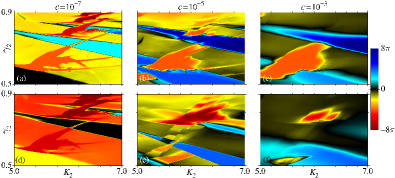
Figure 8: (Color online) Parameter space $(K_{2},\gamma_{2})$ with colors representing the TRC $\mathcal{J}_{T}$ for the system (1). In (a) ($c=10^{-7}$), (b) ($c=10^{-5}$) and (c) ($c=10^{-3}$) the parametric combination $(K_{1},\gamma_{1})=(5.6,0.64)$ [white point D in Fig. 1(a)] was kept fixed, resulting in orbits with period-2 for the map $\mbox{\bf RM}^{(1)}$ and in a RC $\mathcal{J}_{1}\approx-2\pi$, according to Table 1. In (d) ($c=10^{-7}$), (e) ($c=10^{-5}$) and (f) ($c=10^{-3}$) the parametric combination $(K_{1},\gamma_{1})=(6.1,0.81)$ [white point E in Fig. 1(a)] was kept fixed, resulting in orbits with period-2 for the map $\mbox{\bf RM}^{(1)}$ and in a RC $\mathcal{J}_{1}\approx-4\pi$, according to Table 1.

V Conclusions

Recently it was shown Celestino et al. (2011) that single ratchet devices produce optimal currents when the parameters of the system are chosen inside ISSs which live in the parameter space and generate a stable dynamics. We recall here that the ISSs explain all the relevant dynamics which occurs to the ratchet current, ranging from optimal current, current reversal, temperature induced destruction or enhancement of the current, among others. The present work analyses the relevance of such ISSs in the case of two coupled ratchet devices. Furthermore, our results show that it is possible to use one ratchet device to control the current of the other one, leading to completely unexpected behaviors.

We study numerically some of the different dynamical behaviors of a system composed of two elastically coupled ratchet. Such a system can exhibit, depending on the intensity $c$ of coupling, current reversals (from $\mathcal{J}_{T}>0$ to $\mathcal{J}_{T}<0$ and vice versa), duplication of ISSs, hyperchaos and the coexistence of the different kind of attractors, namely chaotic and periodic, periodic and hyperchaotic, chaotic and hyperchaotic, quasiperiodic and periodic, and more than one periodic attractor. The variety of complex dynamics induced by the interaction between the ratchets can be nicely explained in terms of the ISSs. However, when the value of coupling $c$ between the maps $\mbox{\bf RM}^{(1)}$ and $\mbox{\bf RM}^{(2)}$ increases, optimal RCs can appear in distinct regions of the parameter space, differently from the case with one uncoupled particle in which high values of RCs are found only inside the ISSs. Finally, the duplication of the ISSs caused by the interacting ratchet (observed using external forces in 1- and 2-dimensional maps Manchein et al. (2017); da Silva et al. (2017); da Silva et al. (2018a) and in continuous-time dynamical systems da Silva et al. (2018b)) is a very interesting results and leads to an intriguing question regarding the dynamics of many particles interacting systems. It is possible to observe multiplication of ISSs when multiple ratchet are weakly coupled? If so, multiple particle coupled ratchet devices should have an almost regular behavior with optimal current. This is subject of future work.

We also mention that in this work we used equal coupling strength $c$ between both ratchet. In case of distinct coupling strengths, say $c_{\rm RM1}\neq c_{\rm RM2}$ (even if one of them is very small), might drastically change the configuration of the attractors and multistable behaviors in phase space. Interesting results about this subject were obtained for two elastically interacting neurons modeled by FitzHugh-Nagumo oscillators coupled to each other Campbell and Waite (2001). There, it was shown that when the coupling strength between neurons are different, multistability still holds, but the attractors configuration is completely changed. A similar scenario is expected in problems involving near identical ratchet oscillators coupled together with different strengths, but it is very difficult to present some generic statement about how its dynamics should be affected. Indeed, further studies on such direction are needed.

Another important issue is the influence of the noise on the current of coupled ratchet particles. In this scenario, it is expected that Levy noise may enhance the transport of particles Li et al. (2017a, b), while for Gaussian noise the total ratchet current tends to zero with increasing noise intensity since the ISSs of the individual maps decrease Manchein et al. (2013); da Silva et al. (2018a).