Approaching the continuum limit: effective rheology during a two-phase flow

Abstract

It is becoming increasingly clear that there is a regime in immiscible two-phase flow in porous media where the flow rate depends on the pressure drop as a power law with an exponent different than one. This occurs when the capillary forces and viscous forces both influence the flow. At higher flow rates, where the viscous forces dominate, the flow rate depends linearly on the pressure drop. The question we pose here is what happens to the non-linear regime when the system size is increased. Based on analytical calculations using the capillary fiber bundle model and on numerical simulations using a dynamical network model, we find that the non-linear regime moves towards smaller and smaller pressure gradients as the system size grows.

1 Introduction

In 1856, Darcy published his famous treatise where the law that flow rate is proportional to a pressure drop when a fluid flow through a porous medium, was first presented [1]. Eighty years later, the Darcy law was generalized to the simultaneous flow of two immiscible fluids by Wyckoff and Botset [2]. The basic idea behind this generalization is that each fluid sees an available space in which it can flow which consists of the pore space minus the space the other fluid occupies. Each fluid then obeys the Darcy law within this diminished pore space. This idea is clearly oversimplified. It remains to date, however with some important addenda such as the incorporation of capillary effects [3], the dominating tool for simulations of immiscible two-phase flow in porous media. This is in spite of numerous attempts over the years at improving this approach or substitute it for an entirely new approach [4, 5, 6, 7, 8, 9, 10, 11, 12, 13, 14, 15, 16, 17, 18, 19, 20, 21, 22, 23, 24, 25].

A simpler question may be posed when generalizing the Darcy equation to immiscible two-phase flow in porous media. Rather than asking for the flow rate of each of the two fluids, how does the combined flow react to a given pressure drop? It has since Tallakstad et al. [26, 27] did their experimental study of immiscible two-phase flow under steady-state conditions in a Hele-Shaw cell filled with fixed glass beads becomes increasingly clear that there is a flow regime in which the flow rate is proportional to the pressure drop with power different than one [28, 29, 30, 31, 32, 33, 34, 35]. That is, the two immiscible fluids flowing at the pore scale act at the continuum scale as a single non-Newtonian fluid, or more precisely a Herschel-Bulkley fluid where the effective viscosity depends on the shear rate, and hence the flow rate, as a power law [36].

In the experimental setups that have been used, the flow rate of each fluid into the porous medium is controlled and the pressure drop across the porous medium is measured. This leads to at least one of the fluids percolating even at very low flow rates. At these low flow rates, the capillary forces are too strong for the viscous forces to move the fluid interfaces, resulting in the standard linear Darcy law prevailing. As the flow rates are increased, Gao et al. [33] report a regime occurring where there are strong pressure fluctuations but still the linear Darcy law is seen. Then, at even higher flow rates, non-linearity sets in, and a power law relation between flow rate and pressure drop is measured. This non-linearity may be associated with the gradual increase in mobilized interfaces as the flow rates increase [27, 30]. Lastly, at very high flow rates, the capillary forces become negligible compared to the viscous forces, and again, the system reverts to obey a linear Darcy law [31].

A simplified problem compared to that of immiscible two-phase flow in porous media is that of bubbles flowing in a single tube [37, 38, 39, 40]. Sinha et al. [37] studied a bubble train in a tube with a variable radius assuming no fluid films forming. The main result was that the time-averaged flow rate depends on the square root of the excess pressure drop, that is the pressure drop along the tube minus a depinning — or threshold pressure $P_{t}$. Xu and Wang [38] also identified a threshold pressure in their numerical simulations. However, this threshold pressure has a different character from that in the previous study: It is the pressure drop at which contact lines start getting mobilized. The movement of the contact lines consumes energy leading to the effective permeability dropping. Xu and Wang [38] suggest that this is the main mechanism responsible for the non-linearity in the flow-pressure relationship. Lanza et al. considered an immisible mixture of a non-Newtonian and a Newtonian fluid moving along the tube [39], whereas Cheon et al. considered a mixture of compressible and incompressible fluids moving along the tube [40]. In both cases, a non-trivial power law dependence between the flow rate and pressure drop.

The question of whether there should be a threshold pressure or not in the non-linear regime is an important one as assuming there to be one may alter significantly the measured value of the exponent $\beta$ seen in the non-linear regime where

$$Q\sim\begin{cases}0\;,&{\rm if}\ |\Delta P|\leq P_{t}\;,\\ (|\Delta P|-P_{t})^{\beta}\;,&{\rm if}\ |\Delta P|>P_{t}\;,\\ \end{cases}$$ (1)

where $Q=Q_{w}+Q_{n}$ is the volumetric flow rate consisting of the sum of volumetric flow rates of the wetting fluid $Q_{w}$, and the non-wetting fluid $Q_{n}$. $\Delta P$ is the pressure drop across the sample. The value of $\beta$ varies in the literature. Tallakstad et al. [26, 27] reported $\beta=1/0.54=1.85$ (in these papers the inverse exponent was reported), Rassi et al. [29] reported a range of values, $\beta=1/0.3=3.3$ to $\beta=1/0.45=2.2$, and [33] reported $\beta=1/0.6=1.67$. These results are based on experiments and they all assume $P_{t}=0$. Sinha et al. [31] report for their experiments $\beta=1/0.46=2.2$, based on there is a threshold. Sinha and Hansen [30] in numerical work also assumes a threshold pressure based on a dynamic network simulator [41], where fluid interfaces are moved according to the forces they experience [42, 43, 44, 45], and found $\beta=1/0.51=2.0$. The network representing the porous medium was here a disordered square lattice. They followed this up with an effective medium calculation yielding $\beta=2$. Sinha et al. [31] reported $\beta=1/0.50=2.0$ to $\beta=1/0.54=1.85$ based on numerical studies with reconstructed porous media using the same numerical model as in [30]. Yiotis et al. [32] propose $\beta=3/2$ based on numerical work and assuming the existence of a threshold pressure. Recently Fyhn et al. [35] have studied a network model for a mixture of grains with opposite wetting properties with respect to the two immiscible fluids. Depending on the filling ratio between the two grain types, there is a regime where there is no threshold pressure. They find an exponent $\beta=2.56$ in this regime.

There is a lesson to be learned from the study of a very different problem. In 1993 Måløy et al. [46] published an experimental study where a rough hard surface was pressed into a soft material with a flat surface, measuring the force as a function of the deformation. At first contact, the Hertz contact law was seen, i.e., the force depended on the deformation to the 3/2 power. As the deformation proceeded, a different power law emerged, however not in the deformation but in the deformation minus a threshold deformation. And here is the lesson: the threshold deformation was not the deformation at first contact where the Hertz contact law was seen. Transferring this result to the non-linear Darcy case, our point is that the threshold pressure that shows up in the power law does not have to be the pressure needed to get the fluids flowing. The power law (1) may be followed down to a certain pressure difference larger than $P_{t}$. At this pressure difference, there may then be a crossover to a different regime controlled by different physics, e.g., a linear one as Guo et al. [33] reported.

In this paper, we will discuss another aspect of the non-linear flow regime which so far has not been touched upon. So far, the system sizes that have been used in establishing the existence of the non-linear regime, even if the details are not yet sorted out, are limited. This applies both to the experimental and numerical studies that have been published. The question we pose here is: what happens to the non-linear regime when the scale up the system, i.e., we go to the continuum limit? Does the threshold pressure $P_{t}$ remain constant, increase or does it shrink away? Does crossover to the linear Darcy regime remain fixed at a given pressure gradient or changes?

Our conclusion, based on numerical evidence from the dynamic network model [42, 43, 44] and on analytic calculation using the capillary fiber bundle model [47], is that the non-linear regime shrinks away with increasing system size.

In the next section, we present a scaling analysis of the Darcy law and the non-linear regime that sets the stage for the study that follows. We then turn in Section III to the capillary fiber bundle model. Section IV contains our numerical study based on scaling up the square lattice. The last section contains a discussion of the arguments presented earlier in the paper together with our conclusion.

2 Scaling analysis

We assume a porous medium sample that has length $L$ and an transversal area $A$. There is a pressure drop $\Delta P$ across it and this generates a volumetric flow rate of $Q$. When the flow rate is high so that capillary forces may be neglected, the constitutive relation between $Q$ and $\Delta P$ is given by the Darcy law,

$$Q=-M_{d}\Delta P\;,$$ (2)

where $M_{d}$ is the mobility. We introduce the Darcy velocity

$$v=\frac{Q}{A}\;,$$ (3)

and the pressure gradient

$$p=\frac{\Delta P}{L}\;.$$ (4)

The Darcy equation then takes the form

$$v=-m_{d}\ p\;,$$ (5)

where

$$m_{d}=\frac{M_{d}L}{A}\;.$$ (6)

Equations (5) and (6) are both independent of the transversal area $A$ and the length $L$ of the sample.

As has been described in the Introduction, there is a regime in which the volumetric flow rate $Q$ depends on the pressure drop $\Delta P$ as a power law,

$$Q=-M_{\beta}\ {\rm sign}(\Delta P)\Theta(|\Delta P|-P_{t})(|\Delta P|-P_{t})^{\beta}\;,$$ (7)

where $M_{\beta}$ is the non-linear mobility and $P_{t}$ is a threshold pressure. Here $\Theta(|\Delta P|-P_{t})$ is the Heaviside function which is one for positive arguments and zero for negative arguments. We use the Heaviside function to mark the end of the non-linear regime when the pressure drop is lowered. There may be a crossover to a different regime before reaching this lower cutoff [33].

We have in the Introduction pointed out that the non-linear regime, (7), crosses over to the ordinary linear Darcy law behavior above a maximum pressure difference, which we will call $P_{M}$. In the following, we will assume that $P_{t}$ and $P_{M}$ have the same dependence on the system sizes $A$ and $L$. We will support this assumption in the next section where we study the capillary fiber bundle model.

We express the non-linear Darcy law (7) in terms of the Darcy velocity and the pressure gradient,

$$v=-m_{\beta}\ {\rm sign}(p)\Theta\left(|p|-p_{t}\right)\left(|p|-p_{t}\right)^{\beta}\;,$$ (8)

where

$$p_{t}=\frac{P_{t}}{L}\;,$$ (9)

and

$$p_{M}=\frac{P_{M}}{L}\;.$$ (10)

We then have that

$$m_{\beta}=\frac{M_{\beta}L^{\beta}}{A}\;.$$ (11)

The continuum limit is reached by setting $A\sim L^{d-1}\to\infty$, where $d$ is the dimensionality of the sample, and letting $L\to\infty$. In the Darcy regime, equations (2) to (6), $v$, $p$ and the mobility $m_{d}$ are independent of $L$. The non-linear regime is different. The non-linear regime where the constitutive equation (8) applies, $v$ and $p$ are also independent of $L$. However, this is not the case for the threshold pressure $p_{t}$, the crossover pressure $p_{M}$, and the mobility $m_{\beta}$.

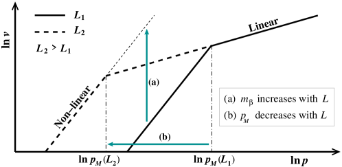
Figure 1: We show $\ln v$ vs. $\ln p$ in both the linear range, equation (5), and the non-linear range, equation (8). Extrapolating the linear part of the curve to $\ln p=0$, it will cross the $\ln v$ axis at $\ln m_{d}$, where $m_{d}$ is the Darcy mobility (6). Extrapolating the non-linear part of the curve to $\ln p=0$, it will cross the $\ln v$ axis at $\ln m_{\beta}$, where $m_{\beta}$ is the non-linear mobility (11). The linear mobility $m_{d}$ does not depend on the system size $L$. However, as we shall see, the non-linear mobility $m_{\beta}$ grows with increasing $L$, see arrow marked (a). This means that the crossover pressure $p_{M}$, where the linear and non-linear part of the curve $\ln v$ vs. $\ln p$ cross moves to the left in the figure, illustrated with arrow (b). Hence, $p_{M}$ decreases with increasing $L$. We have set the threshold pressure $p_{t}$ to zero in this figure.

We note that if $m_{\beta}\to\infty$ and $p_{t}\to 0$ as $L\to\infty$ as $A\sim L^{d-1}\to\infty$, the non-linear regime vanishes in the continuum limit. One may see this by sketching the Darcy law (5) as a straight line in a log-log plot of $v$ vs. $p$ as illustrated in figure 1. The non-linear regime will give another straight line in this diagram with slope $\beta$ when we ignore the threshold correction $|p|-p_{t}\to|p|$. We have $\beta>1$ so that the two lines cross each other with the non-linear line below the Darcy line to the left and above to the right. The system follows the lowest of the two lines for any $|p|$. If now the non-linear $m_{\beta}$ mobility increases with increasing $L$, the cross point between the two lines moves to the left, with the result that the non-linear regime moves to lower and lower value of the pressure gradient $p$ as seen in figure 1.

The reader should note a subtlety here. If $m_{\beta}\to\infty$ as $L\to\infty$ and $A\to\infty$, then we must have the crossover pressure $p_{M}\to 0$ as a consequence. This makes it unnecessary to measure $p_{M}$ — a quantity that is very difficult to measure with any accuracy; it is enough to measure $m_{\beta}$, and not $p_{M}$.

3 Capillary Fiber Bundle Model

We now consider the capillary fiber bundle model [48, 49] as this is a system that can be solved analytically. This model consists of $N$ parallel capillary tubes of equal length $L$. The average transversal area of each tube is $a$ so that $A=Na$. The radius of each tube varies with the position along its axis. We follow the approach of Sinha et al. [37] assuming that the radius $r$ varies as

$$r(x)=\frac{r_{0}}{1-b\cos(2\pi x/l)}\;,$$ (12)

where $r_{0}=\sqrt{a/\pi}$ is the average radius, $0<x<L$ is the position along the capillary fiber and $l$ is the period of the radius variation. The capillary tube is filled with bubbles. Neither of the two immiscible fluids wet the tube walls completely so that there are no films. We now focus on one bubble of the less-wetting fluid. The bubble is limited by interfaces at $x_{I}<x_{F}$ so that the length of the bubble is $\Delta x_{B}=x_{F}-x_{I}$ and the position of its center of mass is $x_{B}=(x_{I}+x_{F})/2$. The capillary pressure drop at $x=x_{I}$ is

$$\frac{2\sigma}{r(x_{I})}=+\frac{2\sigma}{r_{0}}\ \left[1-b\cos\left(\frac{2\pi}{l}x_{I}\right)\right]\;,$$ (13)

and the capillary pressure drop at $x_{f}$ is

$$\frac{2\sigma}{r(x_{F})}=-\frac{2\sigma}{r_{0}}\ \left[1-b\cos\left(\frac{2\pi}{l}x_{F}\right)\right]\;,$$ (14)

where $\sigma$ is the surface tension. The sum of these two forces gives the capillary force on the bubble,

$$p_{c}(x_{B})=-\frac{4b\sigma}{r_{0}}\ \sin\left(\frac{\pi}{l}\Delta x_{B}\right)\sin\left(\frac{2\pi}{l}x_{B}\right)\;.$$ (15)

Suppose now there are $k$ bubbles per unit length in the capillary tube so that it contains $K=kL$ bubbles. At the time $t$ their centers of mass are positioned at $x_{i}(t)$, where $1\leq i\leq K$. The equation of motion for bubble number $i$ is

$$\dot{x}_{i}=-\frac{r_{0}^{2}}{8L\mu_{\rm eff}}\left[\Delta P+\sum_{i=1}^{K}\frac{4b\sigma}{r_{0}}\sin\left(\frac{\pi}{l}\Delta x_{i}\right)\sin\left(\frac{2\pi}{l}x_{i}\right)\right]\;,$$ (16)

where $\mu_{\rm eff}=\mu_{n}\sum_{i=1}^{K}\Delta x_{i}+\mu_{w}(L-\sum_{i=1}^{K}\Delta x_{i})$, in which $\mu_{n}$ is the viscosity of the non-wetting fluid and $\mu_{w}$ is the viscosity of the wetting fluid. We now introduce relative coordinates $\delta x_{i}=x_{i}-x_{0}$ where $x_{0}$ is some chosen point along the abscissa. We have that $\dot{x}_{0}=\dot{x}_{1}=\cdots=\dot{x}_{K}$. This implies that $\delta x_{i}=0$ for all $i$. We may then write the $K$ equations of motion (16) as a single equation

$$\dot{x}_{0}=-\frac{r_{0}^{2}}{8L\mu_{\rm eff}}\left[\Delta P+\Gamma_{s}\sin\left(\frac{2\pi}{l}x_{0}\right)+\Gamma_{c}\cos\left(\frac{2\pi}{l}x_{0}\right)\right]\;,$$ (17)

where

$$\Gamma_{s}=\frac{4b\sigma}{r_{0}}\ \sum_{i=1}^{K}\sin\left(\frac{\pi}{l}\Delta x_{i}\right)\sin\left(\frac{\pi}{l}\delta x_{i}\right)\;,$$ (18)

and

$$\Gamma_{c}=\frac{4b\sigma}{r_{0}}\ \sum_{i=1}^{K}\sin\left(\frac{\pi}{l}\Delta x_{i}\right)\cos\left(\frac{\pi}{l}\delta x_{i}\right)\;,$$ (19)

Let us set

$$P_{t}=\sqrt{\Gamma_{s}^{2}+\Gamma_{c}^{2}}\;,$$ (20)

and introduce the non-dimensional variables for $x_{0}$ and $t$,

$$\theta=\frac{2\pi}{l}x_{0}\;,$$ (21)

and

$$\tau=\frac{\pi r_{0}^{2}P_{t}}{4Ll\mu_{\rm eff}}\ t\;.$$ (22)

Hence, equation (17) becomes

$$\dot{\theta}=\frac{\Delta P}{P_{t}}-\sin\left(\theta+\theta_{t}\right)\;,$$ (23)

where

$$\tan(\theta_{t})=\frac{\Gamma_{s}}{\Gamma_{c}}\;.$$ (24)

We see from this equation that $|\Delta P|$ must be larger than $P_{t}$ for the bubbles to move in the capillary tube; $P_{t}$ is a threshold pressure.

(In references [37] and [47] there is an error in identifying the mathematical form of the threshold pressure. This error has no impact on the results there.)

We now assume we scale $L$ in such a way that $k=K/L$ remains constant. How will $P_{t}$ scale with $L$? Since the number of interfaces increase linearly with $L$, one may be tempted to believe that $P_{t}$ scales with $L$. However, the interfaces come in pairs, one for each bubble, and the capillary pressure drops across the interfaces come with opposite signs. Hence, the capillary pressure $p_{c}(x_{B})$ in equation (15) can have either sign depending on the size and position of the bubble, $\Delta x_{B}$ and $x_{B}$. With $K$ bubbles, $\Gamma_{s}$ and $\Gamma_{c}$ are sums of factors that have random signs; we are dealing with random walks. As a consequence, we have that

$$P_{t}\sim\sqrt{L}\;.$$ (25)

A more general version of this argument has been presented in [50].

We now bring together $N$ of these capillary fibers to form a bundle [47]. The fibers have radii $r_{0}$ drawn from some probability distribution. Since the thresholds $P_{t}$ are inversely proportional to $r_{0}$, we will consider the corresponding threshold probability distribution. We follow [47] and consider first the cumulative probability

$$\Pi(P^{\prime}_{t})=\left\{\begin{array}[]{ll}0&\mbox{, $P_{t}\leq 0$\;,}\\ \frac{P^{\prime}_{t}}{P_{M}}&\mbox{, $0<P^{\prime}_{t}\leq P_{M}$\>,}\\ 1&\mbox{, $P_{t}>P_{M}$\;,}\\ \end{array}\right.$$ (26)

where $P_{M}$ is the maximum threshold. Note the change in notation: The threshold associated with a given capillary fiber is $P^{\prime}_{t}$. We reserve $P_{t}$ for the threshold pressure the whole capillary fiber bundle. Averaging the equation of motion (17) for each fiber in the bundle then gives [47]

$$Q=-\frac{aA}{32\mu_{\rm eff}L}\left|\frac{\Delta P}{P_{M}}\right|\Delta P$$ (27)

when $|\Delta P|\leq P_{M}$. Hence, the threshold pressure $P_{t}=0$ when the threshold distribution for the individual fibers is given by (26). Hence, we have that

$$M_{\beta}=\frac{aA}{32\mu_{\rm eff}P_{M}L}\;.$$ (28)

In terms of the Darcy velocity $v$ and the pressure gradient $p$, this expression becomes

$$v=-\frac{a}{32\mu_{\rm eff}\ p_{M}}\ |p|\ p=-m_{\beta}\ |p|\ p\;,$$ (29)

where $p_{M}=P_{M}/L$. Hence, $\beta=2$. We see that $m_{\beta}$ has the same form as in equation (11),

$$m_{\beta}=\frac{a}{32\mu_{\rm eff}\ p_{M}}=\frac{M_{\beta}L^{2}}{A}\frac{1}{p_{M}}\;.$$ (30)

$P_{M}$ is the threshold pressure for getting the fluid in the most difficult fiber to flow. Hence, we will have that

$$p_{M}=\frac{P_{M}}{L}\sim\frac{1}{\sqrt{L}}\;,$$ (31)

from equation (25), and as a consequence

$$m_{\beta}\sim L^{1/2}\;.$$ (32)

It is important to note that $P_{t}=0$ in this fiber bundle. Thus, we have $p_{t}=0$ and $m_{\beta}\to\infty$ in the limit $A\to\infty$ and $L\to\infty$: The non-linear behavior disappears in the continuum limit, see figure 1.

We now consider the cumulative threshold probability [47]

$$\Pi(P_{t})=\left\{\begin{array}[]{ll}0&\mbox{, $P^{\prime}_{t}\leq P_{t}$\;,}\\ \frac{P^{\prime}_{t}-P_{t}}{P_{M}-P_{t}}&\mbox{, $P_{t}<P^{\prime}_{t}\leq P_{M}$\>,}\\ 1&\mbox{, $P^{\prime}_{t}>P_{M}$\;,}\\ \end{array}\right.$$ (33)

noting that such a distribution is more realistic than one where the minimum threshold is zero, see the distribution in equation (26). This is so since a zero threshold would mean that there is a possibility for an infinite radius $r_{0}$ in equations (13) and (14).

The flow rate is in this case given by

$$Q=-\frac{aA\ {\rm sign}(\Delta P)}{3\sqrt{2}\pi\mu_{\rm av}L}\frac{\sqrt{P_{t}}}{(P_{M}-P_{t})}(|\Delta P|-P_{t})^{3/2}\;,$$ (34)

for $|\Delta P|$ close to but larger than the threshold $P_{t}$. In terms of the Darcy velocity and pressure gradient, this expression becomes

$$v = -\frac{a\ {\rm sign}(p)}{3\sqrt{2}\pi\mu_{\rm av}}\frac{\sqrt{p_{t}}}{(p_{M}-p_{t})}(|p|-p_{t})^{3/2}$$ (35)

$$= -m_{\beta}\ {\rm sign}(p)\ (|p|-p_{t})^{3/2}\;,$$

where we have defined

$$p_{t}=\frac{P_{t}}{L}\;.$$ (36)

Since $P_{t}$ is the threshold pressure for the capillary fiber with the smallest threshold in the bundle, we must have

$$p_{t}\sim\frac{1}{\sqrt{L}}\;,$$ (37)

from equation (25). Combined with (31), we find

$$m_{\beta}\sim L^{1/4}\;.$$ (38)

Hence, we find that $p_{t}\to 0$ and $m_{\beta}\to\infty$ in the limit $A\to\infty$ and $L\to\infty$: The non-linear behavior disappears also in this case in the continuum limit.

Even though, we have found that $m_{\beta}$ to increase with $L$ based on the capillary fiber bundle model, we believe this result to be generally applicable. The reason for this is that the fluctuations of surface tension of the interfaces keeping the fluids in place scale more slowly than the pressure gradient. This is a mechanism that will be present also in porous media, and not just in the capillary fiber bundles.

4 Numerical results based on a dynamic network model

We base our simulations on the dynamic network simulator described in [42, 43, 44]. It consists of interfaces that span the pores and move according to the pressure gradient they experience. Hence, no wetting films occur in the simulations. We use a square lattice oriented at $45^{\circ}$ to the average flow direction. We assume periodic boundary conditions both in the direction orthogonal to the average flow direction and in the direction parallel to the average flow.

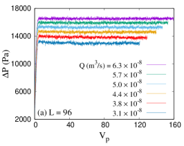
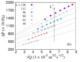
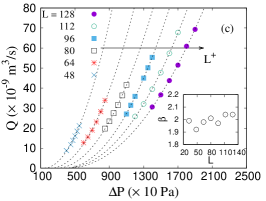
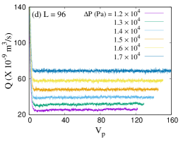
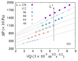
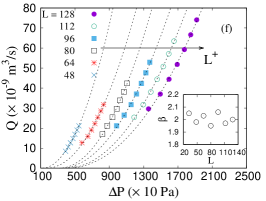
Figure 2: The upper panel of the figure corresponds to the constant flow rate while the lower panel corresponds to constant pressure gradient. The size of the network used is $96\times 96$. The saturation $S_{w}$ value is kept constant at 0.5. (a) & (d) At a constant flow rate ($3.0\times 10^{-8}<Q<6.5\times 10^{-8}$ m³/s) or pressure gradient ($1.2\times 10^{4}<\Delta P<1.7\times 10^{4}$ Pa), $\Delta P$ and $Q$ gradually approaches the steady-state value with increasing pore volumes $V_{p}$. (b) & (e) We assume $\beta=2.0$. The figures show the variation of $\Delta P$ with $\sqrt{Q}$ at a constant flow rate (upper) and constant pressure gradient (lower). For both figures the system sizes from up to down are 128, 112, 96, 80, 64, and 48. As the size of the system is increased both the slope of the straight line and the intercept on the ordinate increases. The value of $P_{t}$ and $M_{\beta}$ can be extracted from the intercept of the straight the line on the ordinate and its slope respectively (see equation 39). (c) & (f) $\beta$ is treated to be a fitting parameter and the numerical results are fitted with the equation (7) to find $\beta$, $M_{\beta}$ and $P_{t}$. The system sizes used here are the same as (b) and (e). The fitted $\beta$ value is observed to be close to $2.0$ (shown in the inset).

The square lattices we have used range in size between $48\times 48$ and $208\times 208$. All the links are of length $l=10^{-3}$ m with its average radius $r$ chosen randomly between $0.1l$ and $0.4l$. The simulation is carried out at both constant flow rate $Q$ and constant pressure gradient $\Delta P$, kept at a certain low value so that the capillary forces dominate and the relationship between $Q$ and $\Delta P$ is non-linear. For system sizes $L=48$, 64, 80, 96, 112, 128, 144, 160, 176, 192, and 208 we have used respectively 20, 20, 15, 15 10, 10, 8, 5, 3, 3, and 3 realizations. We set the surface tension $\sigma$ to the value 0.03 or 0.01 N/m. While calculating the flow rate, instead of assuming a cross-section, we summed up the flow rate for all links and divided it by the total number of links.

Figure 3: $p_{t}$ as a function of $L$ where $L$ ranges from 48 to 176 is shown for (a) constant pressure gradient and $\beta=2.0$ as well as treating $\beta$ as a fitting parameter; (b) $\beta$ as a fitting parameter for both constant pressure and constant flow rate. The inset in both figures shows the size effect for $P_{t}$ under the same conditions. The saturation $S_{w}=0.5$ in all cases.

Figure 2 shows the relation between the pressure gradient and the flow rate when the model reaches the steady state. The upper panels of the figure correspond to constant $Q$ while the lower panels show the results for constant $\Delta P$. We show in figure 2(a) pressure difference $\Delta P$ as a function of injected pore volumes when keeping $Q$ constant and in figure 2(d) $Q$ as a function of injected pore volumes when keeping $\Delta P$ constant. We see that in both cases, within a few injected pore volumes the system reaches a steady state. All data are collected after the system reaches a steady state. For the flow rates shown the system is well within the non-linear region where the equation (7) applies.

In order to calculate $P_{t}$ for a system size $L$ we have adopted two different methods. For the first one we have assumed the mean-field solution from Sinha and Hansen [30], setting $\beta=2$ in equation (7). For the second method, we keep $\beta$ free as a fitting parameter and the numerical results are fitted with equation (7) with variables $P_{t}$, $M_{\beta}$ and $\beta$. We do not measure the crossover pressure $P_{M}$ where the non-linear relation (7) is replaced by the Darcy law (2). As we have already observed at the end of Section II, this is not necessary when we determine $P_{t}$ and $M_{\beta}$.

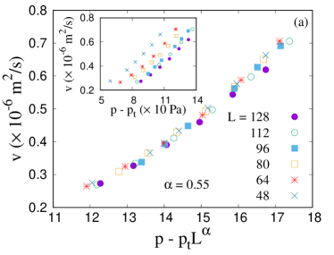
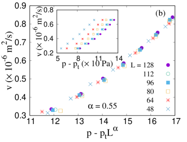
Figure 4: Darcy velocity $v=Q/L$ plotted against $p-p_{t}L^{\alpha}=\Delta P/L-(P_{t}/L^{1+\alpha})L^{\alpha}$, where we have set $\alpha=0.55$, thus producing data collapse. We assumed $\beta$ to be a fitting parameter. We furthermore set $\mu_{n}/\mu_{w}=1.0$ and $S_{w}=0.5$ respectively. The study was carried out for (a) constant pressure gradient and (b) constant flow rate.

Constant $\beta=2$: In the capillary force dominated region, if we assume $\beta=2$, we get from equation (7) that

$$\Delta P\sim\sqrt{\frac{Q}{M_{\beta}}}+P_{t}\;,$$ (39)

when taking into account the sign of $\Delta P$ used in the simulation. Figures 2(b) and (e) show how the pressure gradient $\Delta P$ behaves with $\sqrt{Q}$ for constant flow rate and constant pressure gradient respectively. In both cases, we observe a straight line whose intercept on ordinate gives the value of $P_{t}$. As we increase $L$, the slope of the straight line as well as the intercept $P_{t}$ increases. $M_{\beta}$ can be extracted from the slope of this straight line.

$\beta$ as fitting parameter: Next, we have kept $\beta$ as a free parameter and the numerical results are fitted with the equation (7). The fitted results are shown by dotted lines in figure 2(c) and (f). The inset in the same figure shows the $\beta$ values for different system sizes. The variation in $\beta$ values show that the mean-field approximation is valid for our numerical results and $\beta$ has a value close to 2.0.

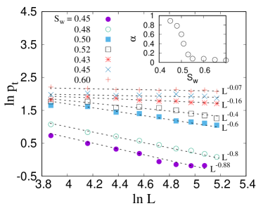
Figure 5: Here we show $p_{t}=P_{t}/L$ as a function of $L$ for $L=48$ to $L=176$, $\mu_{n}/\mu_{w}=1.0$ and for different values of $S_{w}$. The behavior is consistent with equation (40). The exponent $\alpha$ is a strong function of $S_{w}$. However, all values of $\alpha$ are negative so that $p_{t}\to 0$ as $L\to\infty$.

We now discuss the size effect of the threshold pressure $p_{t}=P_{t}/L$. In figure 3(a) we show $p_{t}$ as a function of $L$ for constant pressure gradient $\Delta P$ for the following two cases: $\beta=2$, as well as when we keep $\beta$ as an independent fitting parameter. In both cases, a scale-free decay of $p_{t}$ is observed with $L$. Figure 3(b) shows the same power law decay for both constant $\Delta P$ and constant flow rate $Q$ with $\beta$ being treated as an independent fitting parameter. We find in all cases

$$p_{t}\sim L^{-\alpha}\;,$$ (40)

where $\alpha=0.55$. We will, however, demonstrate later on that $\alpha$ depends on the saturation $S_{w}$.

Another way of displaying the dependence of the threshold pressure $p_{t}$ on the system size $L$ is to plot the Darcy velocity $v$ as a function of $p-p_{t}L^{\alpha}$. We should then observe data collapse for different values of $L$. This is precisely what we observe in figure 4. We note that whether we keep the pressure drop $\Delta P$ or the flow rate $Q$ constant, the results are quite similar. In light of this behavior, we will only consider the constant pressure drop scenario in the following. We will also in the following keep $\beta$ as a free parameter.

The dependence of $p_{t}$ on saturation $L$ for various saturation $S_{w}$ is shown in figure 5. We observe $\alpha$ to remain constant at a low value for $S_{w}>0.55$. In the region $0<S_{w}<0.55$, $\alpha$ increases quickly with decreasing saturation. The variation $\alpha$ with $S_{w}$ is shown in the inset of figure 5. In all cases, $\alpha$ is positive so that $p_{t}\to 0$ as $L\to\infty$.

These results show that the capillary fiber bundle model which predicts $\alpha=1/2$ does not capture the full mechanisms behind the scaling we observe. We will return to this in the concluding section.

We now turn to the mobility $M_{\beta}$ and $m_{\beta}$ defined in equations (7) and (11) respectively. Figure 6 shows the size effect for both $M_{\beta}$ and $m_{\beta}$.

$$M_{\beta}\propto L^{-\eta}$$ (41)

where $\eta$ has values 0.78 ($S_{w}=0.53$), 0.82 ($S_{w}=0.50$) and 0.75 ($S_{w}=0.48$), hence the dependence on saturation. From equation (11), we have that

$$m_{\beta}=\frac{M_{\beta}}{L}L^{\beta}\sim L^{\beta-1-\eta}\;,$$ (42)

where we have used that $A=L$ for the two-dimensional networks we use. With the value $\beta=2.0$, we find that $\beta-1-\eta$ is larger than zero for all observed $\eta$-values. More specifically, we find $\beta-1-\eta=0.22$, $0.18$ and $0.25$ respectively. We show these results in figure 6.

We note how close the exponents measured in figure 6b are to the capillary fiber bundle model, equation (38), where an exponent 1/4 was found.

5 Discussion and conclusion

We have in this paper posed the question: Does the non-linear regime where the flow rate depends on the pressure drop through a power law with exponent different expand its range of validity, diminish it or stay the same? We have used two approaches to answer this question. The first one is to solve the capillary fiber bundle model. In doing so, we find that indeed the non-linear regime shrinks away with increasing system size. The reason for this is that the crossover pressure that defines the border between the non-linear regime and the linear Darcy regime moves toward zero with increasing system size. This, in turn, is a result of this threshold pressure $p_{M}$ is a sum of factors that appear with random signs, thus rendering it into a random walk process. The mobility $m_{\beta}$ depends on the inverse threshold pressure to a power. This ensures that it increases when the threshold pressure decreases, a necessary and sufficient condition for the non-linear regime to shrink away.

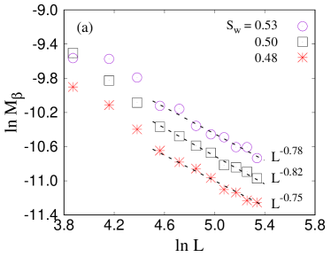
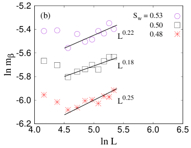
Figure 6: The mobility $M_{\beta}$ defined in equation (7) scales with system size $L$, ranging from $L=48$ to $L=208$, as described in equation (41). The scaled mobility (11) then scales as $m_{\beta}=M_{\beta}L^{\beta-1}\sim L^{\beta-1-\eta}$. Since $\eta<1$ and $\beta\approx 2.0$, $m_{\beta}$ increases with increasing $L$. We set $\mu_{n}/\mu_{w}=1.0$ here.

We find the same qualitative behavior in the dynamic network model we then employ: the threshold pressure $p_{t}$ shrinks and the mobility $m_{\beta}$ increases with increasing system size. Both quantities depend on the system size according to a power law. We find that the exponents depend weakly on the saturation $S_{n}$. However, they are quite close to the values found in the capillary fiber bundle model when we assume that the capillary threshold $P_{t}$ distribution does not go all the way to zero, see equation (26), a feature also present in the dynamic pore network model. Compare the exponents observed in figure 6 with the scaling found for the mobility $m_{\beta}$ for the capillary fiber bundle model, equation (38).

We urge that experiments are done in order to move beyond the theoretical and numerical considerations presented here with their obvious limitations.

An understanding of the non-linear Darcy regime is very important as it occurs right in the parameter range relevant for many industrial situations such as oil recovery, water flow in aquifers etc. It should be noted that all theories for immiscible two-phase flow based on refining the relative permeability approach will be unable to handle this non-linearity. Hence, it presents a huge challenge to the porous media community.

Declaration — The authors declare no conflict of interest.

Acknowledgement — The authors thank Dick Bedeaux, Carl Fredrik Berg, Eirik G. Flekkøy, Signe Kjelstrup, Knut Jørgen Måløy, Per Arne Slotte and Ole Torsæter for interesting discussions. This work was partly supported by the Research Council of Norway through its Centres of Excellence funding scheme, project number 262644.

References

- [1] H. P. G. Darcy, Les Fontaines publiques de la ville de Dijon. Exposition et application des principes à suivre et des formules à employer dans les questions de distribution d’eau, Victor Dalamont, Paris, 1856.
- [2] R. D. Wyckoff and H. G. Botset, The flow of gas-liquid mixtures through unconsolidated sands, Physics 7, 325-345 (1936); doi.org/10.1063/1.1745402.
- [3] M. C. Leverett, Capillary Behavior in Porous Solids, Trans. AIMME, 142, 152 (1941); doi.org/10.2118/941152-G.
- [4] S. M. Hassanizadeh and W. G. Gray, Mechanics and Thermodynamics of Multiphase Flow in Porous Media Including Interphase Boundaries, Adv. Water Res. 13, 169 (1990); doi.org/10.1016/0309-1708(90)90040-B.
- [5] S. M. Hassanizadeh and W. G. Gray, Towards an Improved Description of the Physics of Two-Phase Flow, Adv. Water Res. 16, 53 (1993); doi.org/10.1016/0309-1708(93)90029-F.
- [6] S. M. Hassanizadeh and W. G. Gray, Thermodynamic Basis of Capillary Pressure in Porous Media, Water Resour. Res. 29, 3389 (1993); doi.org/10.1029/93WR01495.
- [7] J. Niessner, S. Berg and S. M. Hassanizadeh, Comparison of Two-Phase Darcy’s Law with a Thermodynamically Consistent Approach, Transp. Por. Med. 88, 133 (2011); doi.org/10.1007/s11242-011-9730-0.
- [8] W. G. Gray and C. T. Miller, Introduction to the Thermodynamically Constrained Averaging Theory for Porous Medium Systems (Springer Verlag, Berlin, 2014).
- [9] S. Kjelstrup, D. Bedeaux, A. Hansen, B. Hafskjold and O. Galteland, Non-Isothermal Transport of Multi-Phase Fluids in Porous Media. The entropy production, Front. Phys. 6, 126 (2018); doi.org/10.3389/fphy.2018.00126.
- [10] S. Kjelstrup, D. Bedeaux, A. Hansen, B. Hafskjold and O. Galteland, Non-Isothermal Transport of Multi-Phase Fluids in Porous Media, Constitutive equations, Front. Phys. 6, 150 (2019); doi.org/10.3389/fphy.2018.00150.
- [11] R. Hilfer and H. Besserer, Macroscopic two-phase flow in porous media, Physica B, 279, 125 (2000); doi.org/10.1016/S0921-4526(99)00694-8.
- [12] R. Hilfer, Capillary pressure, hysteresis and residual saturation in porous media, Physica A, 359, 119 (2006); doi.org/10.1016/j.physa.2005.05.086.
- [13] R. Hilfer, Macroscopic capillarity and hysteresis for flow in porous media, Phys. Rev. E, 73, 016307 (2006); doi.org/10.1103/PhysRevE.73.016307.
- [14] R. Hilfer, Macroscopic capillarity without a constitutive capillary pressure function, Physica A, 371, 209 (2006); doi.org/10.1016/j.physa.2006.04.051.
- [15] R. Hilfer and F. Doster, Percolation as a basic concept for capillarity, Transp. Por. Med. 82, 507 (2009); doi.org/10.1007/s11242-009-9395-0.
- [16] F. Doster, O. Hönig and R. Hilfer, Horizontal Flow and Capillarity-Driven Redistribution in Porous Media, Phys. Rev. E, 86, 016317 (2012); doi.org/10.1007/s11242-009-9395-0.
- [17] M. S. Valavanides, G. N. Constantinides and A. C. Payatakes, Mechanistic Model of Steady-State Two-Phase Flow in Porous Media Based on Ganglion Dynamics, Transp. Porous Media 30, 267 (1998); doi.org/10.1023/A:1006558121674.
- [18] M. S. Valavanides, Steady-State Two-Phase Flow in Porous Media: Review of Progress in the Development of the DeProF Theory Bridging Pore- to Statistical Thermodynamics-Scales, Oil Gas Sci. Technol. 67, 787-804 (2012); doi.org/10.2516/ogst/2012056.
- [19] M. S. Valavanides, Review of Steady-State Two-Phase Flow in Porous Media: Independent Variables, Universal Energy Efficiency Map, Critical Flow Conditions, Effective Characterization of Flow and Pore Network, Transp. Porous Media, 123, 45–99 (2018); doi.org/10.1007/s11242-018-1026-1.
- [20] A. Hansen, S. Sinha, D. Bedeaux, S. Kjelstrup, M. A. Gjennestad and M. Vassvik, Relations Between Seepage Velocities in Immiscible, Incompressible Two-Phase Flow in Porous Media, Transp. Porous Media 125, 565 (2018); doi:10.1007/s11242-018-1139-6.
- [21] S. Roy, S. Sinha and A. Hansen, Flow-area relations in immiscible two-phase flow in porous media, Front. Phys. 8, 4 (2020); doi.org/10.3389/fphy.2020.00004.
- [22] S. Roy, H. Pedersen, S. Sinha and A. Hansen, The Co-Moving Velocity in Immiscible Two-Phase Flow in Porous Media, Transp. Porous Media, 143, 69 (2022); doi.org/10.1007/s11242-022-01783-7.
- [23] A. Hansen, E. G. Flekkøy, S. Sinha and P. A. Slotte, A Statistical Mechanics Framework for Immiscible and Incompressible Two-Phase Flow in Porous Media, Adv. Water Res. 171, 104336 (2023); doi.org/10.1016/j.advwatres.2022.104336.
- [24] H. Pedersen and A. Hansen, Parameterizations of immiscible two-phase flow in porous media, Front. Phys. 11 1127345 (2023); doi.org/10.3389/fphy.2023.1127345.
- [25] H. Fyhn, S. Sinha and A. Hansen, Local statistics of immiscible and incompressible two-phase flow in porous media, Physica A, 616, 128626 (2023); doi.org/10.1016/j.physa.2023.128626.
- [26] K. T. Tallakstad, H. A. Knudsen, T. Ramstad, G. Løvoll, K. J. Måløy, R. Toussaint, and E. G. Flekkøy, Steady-state two-phase flow in porous media: statistics and transport properties, Phys. Rev. Lett. 102, 074502 (2009); doi.org/10.1103/PhysRevLett.102.074502.
- [27] K. T. Tallakstad, G. Løvoll, H. A. Knudsen, T. Ramstad, E. G. Flekkøy, and K. J. Måløy, Steady-state, simultaneous two-phase flow in porous media: An experimental study, Phys. Rev. E 80, 036308 (2009); doi.org/10.1103/PhysRevE.80.036308.
- [28] M. Grøva and A. Hansen, Two-phase flow in porous media: power-law scaling of effective permeability, J. Phys.: Conf. Series, 319, 012009 (2011); doi.org/10.1088/1742-6596/319/1/012009.
- [29] E. M. Rassi, S. L. Codd and J. D. Seymour, Nuclear magnetic resonance characterization of the stationary dynamics of partially saturated media during steady-state infiltration flow, New J. Phys. 13, 015007 (2011); doi.org/10.1088/1367-2630/13/1/015007.
- [30] S. Sinha and A. Hansen, Effective rheology of immiscible two-phase flow in porous media, EPL, 99, 44004 (2012); doi.org/10.1209/0295-5075/99/44004.
- [31] S. Sinha, A. T. Bender, M. Danczyk, K. Keepseagle, C. A. Prather, J. M. Bray, L. W. Thrane, J. D. Seymour, S. L. Codd and A. Hansen, Effective Rheology of Two-Phase Flow in Three-Dimensional Porous Media: Experiment and Simulation, Transp. Porous Med. 119, 77-94 (2017); doi.org/10.1007/s11242-017-0874-4.
- [32] A. G. Yiotis, A. Dollari, M. E. Kainourgiakis, D. Salin, and L. Talon, Nonlinear Darcy flow dynamics during ganglia stranding and mobilization in heterogeneous porous domains, Phys. Rev. Fluids 4, 114302 (2019); doi.org/10.1103/PhysRevFluids.4.114302.
- [33] Y. Gao, Q. Lin, B. Bijeljic and M. J. Blunt, Pore-scale dynamics and the multiphase Darcy law, Phys. Rev. Fluids 5, 013801 (2020); doi.org/10.1103/PhysRevFluids.5.013801.
- [34] H. Fyhn, S. Sinha, S. Roy and A. Hansen, Rheology of immiscible two-phase flow in mixed wet porous media: Dynamic pore network model and capillary fiber bundle model results, Transp. Porous Media, 139, 491 (2021); doi.org/10.1007/s11242-021-01674-3.
- [35] H. Fyhn, S. Sinha and A. Hansen, Effective rheology of immiscible two-phase flow in porous media consisting of random mixtures of grains having two types of wetting properties, Front. Phys. 11, 1175426 (2023); doi.org/10.3389/fphy.2023.1175426.
- [36] W. H. Herschel and R. Bulkley, Konsistenzmessungen von Gummi-Benzollösungen, Kolloid Zeitschrift, 39, 291 (1926); doi:10.1007/BF01432034.
- [37] S. Sinha, A. Hansen, D. Bedeaux and S. Kjelstrup, Effective rheology of bubbles moving in a capillary tube, Phys. Rev. E 87, 025001 (2011); doi.org/10.1103/PhysRevE.87.025001.
- [38] X. Xu and X. Wang, Non-Darcy behavior of two-phase channel flow, Phys. Rev. E, 90, 023010 (2014); doi.org/10.1103/PhysRevE.90.023010.
- [39] F. Lanza, A. Rosso, L. Talon and A. Hansen, Non-Newtonian rheology in a capillary tube with varying radius, Transp. Porous Media, 145, 245 (2022); doi.org/10.1007/s11242-022-01848-7.
- [40] H. L. Cheon, H. Fyhn, A. Hansen, Ø. Wilhelmsen and S. Sinha, Steady-state two-phase flow of compressible and incompressible fluids in a capillary tube of varying radius, Transp. Porous Media, 147, 15 (2023); doi.org/10.1007/s11242-022-01893-2.
- [41] V. Joekar-Niasar and S. M. Hassanizadeh, Analysis of Fundamentals of Two-Phase Flow in Porous Media Using Dynamic Pore-Network Models: a Review, Crit. Rev. Environ. Sc. Tech. 42, 1895 (2012); doi:10.1080/10643389.2011.5 74101
- [42] E. Aker, K. J. Måløy, A. Hansen and G. G. Batrouni, A Two-Dimensional Network Simulator for Two-Phase Flow in Porous Media, Transp. Porous Media, 32, 163 (1998), doi:10.1023/A:1006510106194.
- [43] M. Aa. Gjennestad, M. Vassvik, S. Kjelstrup and A. Hansen, Stable and Efficient Time Integration of a Dynamic Pore Network Model for Two-Phase Flow in Porous Media, Front. Phys. 6, 56 (2018); doi.org/10.3389/fphy.2018.00056.
- [44] S. Sinha, M. Aa. Gjennestad, M. Vassvik and A. Hansen, Fluid Meniscus Algorithms for Dynamic Pore-Network Modeling of Immiscible Two-Phase Flow in Porous Media, Front. Phys. 8, 548497 (2020); doi.org/10.3389/fphy.2020.548497.
- [45] B. Zhao, C. W. MacMinn, B. K. Primkulov, Y. Chen, A. J. Valocchi, J. Zhao, Q. Kang, K. Bruning, J. E. McClure, C. T. Miller, A. Fakhari, D. Bolster, T. Hiller, M. Brinkmann, L. Cueto-Felgueroso, D. A. Cogswell, R. Verma, M. Prodanovic, J. Maes, S. Geiger, M. Vassvik, A. Hansen, E. Segre, R, Holtzman, Z. Yang, C. Yuan, B. Chareyre and R. Juanes, Comprehensive comparison of pore-scale models for multiphase flow in porous media, Proc. Natl. Acad. Sci. 116, 13799 (2019); doi.org/10.1073/pnas.1901619116.
- [46] K. J. Måløy, X. L. Wu, A. Hansen and S. Roux, Elastic contact on rough fracture surfaces, EPL, 24, 35 (1993); doi.org/10.1209/0295-5075/24/1/006.
- [47] S. Roy, A. Hansen and S. Sinha, Effective rheology of two-phase flow in a capillary fiber bundle model, Front. Phys. 7, 92 (2019); doi.org/10.3389/fphy.2019.00092.
- [48] A. E. Scheidegger, Theoretical models of porous matter, Producers Monthly, August, 17 (1953).
- [49] A. E. Scheidegger, The physics of flow through porous media, University of Toronto Press, Toronto, 1974.
- [50] J. Feder, E. G. Flekkøy and A. Hansen, Physics of Flow in Porous Media, Cambridge University Press, Cambridge, 2022.