Array Languages Make Neural Networks Fast

Abstract.

Modern machine learning frameworks are complex: they are typically organised in multiple layers each of which is written in a different language and they depend on a number of external libraries, but at their core they mainly consist of tensor operations. As array-oriented languages provide perfect abstractions to implement tensor operations, we consider a minimalistic machine learning framework that is shallowly embedded in an array-oriented language and we study its productivity and performance. We do this by implementing a state of the art Convolutional Neural Network (CNN) and compare it against implementations in TensorFlow and PyTorch — two state of the art industrial-strength frameworks. It turns out that our implementation is 2 and 3 times faster, even after fine-tuning the TensorFlow and PyTorch to our hardware — a 64-core GPU-accelerated machine. The size of all three CNN specifications is the same, about 150 lines of code. Our mini framework is 150 lines of highly reusable hardware-agnostic code that does not depend on external libraries. The compiler for a host array language automatically generates parallel code for a chosen architecture. The key to such a balance between performance and portability lies in the design of the array language; in particular, the ability to express rank-polymorphic operations concisely, yet being able to do optimisations across them. This design builds on very few assumptions, and it is readily transferable to other contexts offering a clean approach to high-performance machine learning.

1. Introduction

With the increasing success of machine learning in various domains, scientists attempt to solve more and more complex problems using neural networks and deep learning. Increased complexity in the context of deep learning typically means more layers of neurons and larger training sets all of which results in the necessity to process larger amounts of data. As a result modern networks require advanced and powerful hardware — modern machine learning applications are envisioned to run on massively parallel high-throughput systems that may be equipped with GPUs, TPUs or even custom-built hardware.

Programming such complex systems is very challenging, specifically in an architecture-agnostic way. Therefore, there is a big demand for a system that abstracts away architectural details letting the users to focus on the machine learning algorithms. TensorFlow or PyTorch solve exactly that problem — they provide a convenient level of abstraction, offering a number of building blocks that machine learning scientists can use to specify their problems. Productivity of such a solution is quite high as these frameworks are embedded into high-level languages such as Python or C++.

However, turning a framework-based specification into an efficient code remains challenging. There is a huge semantic gap between the specification and the hardware, yet frameworks such a TensorFlow and PyTorch introduce many levels of abstractions that one needs to deal with. Typically there is a Python front-end, a core library in C++ that depends on numerous external libraries for linear algebra, tensor operations, libraries for GPUs and other specialised hardware. Such a complexity makes it challenging to deliver excellent performance: optimisations across multiple layers of abstraction as well as across multiple external libraries inherently come with overheads.

The key question we are investigating is: can we identify a single layer of abstraction where on the one hand we can express the core building blocks and generate efficient parallel code, and on the other hand that is high-level enough to be used as a front-end.

Based on the observation that neural networks can be concisely expressed as computations on high-ranked tensors, we look into using a shape-polymorphic array language APL (Iverson, 1962) as the central layer of abstraction. While APL itself seems suitable in terms of expressiveness (Šinkarovs et al., 2019) the interpreter-based implementation of operators, non surprisingly, does not readily provide parallel performance anywhere near that of TensorFlow or PyTorch.

However, over the last 50 years we have seen quite some research into compilation of array languages into efficient parallel code (Cann and Feo, 1990; Bernecky, 1997; Scholz, 2003; Henriksen et al., 2017; Steuwer et al., 2017). These languages leverage whole program optimisations and they offer decent levels of parallel performance. They also offer high program portability, as inputs are typically hardware-agnostic and all the decisions on optimisations and code generation are taken by the compiler. A user can influence these decisions by passing options, but no code modifications are required.

For the purposes of this paper we use SaC (Scholz, 2003), a functional array language, as our implementation vehicle. We focus on a simple yet frequently benchmarked CNN for recognising handwritten characters. First we implement building blocks that are required to define a chosen CNN in native SaC and then we use these building blocks to define the network. We compare the resulting code size and performance against TensorFlow and PyTorch. We observe that the overall problem can be expressed concisely (300 lines of native SaC code) and on a GPU-accelerated 64-core machine, our solution performs two and three times faster than the TensorFlow- and PyTorch-based implementations. The key aspect of such good performance is first-class support for multi-dimensional arrays in a functional setting followed by a number of well-known code-generation techniques used by the chosen compiler.

This example suggests that at least for this particular domain, the trade-off between conciseness, performance and development time is quite satisfying.

The individual contributions of the paper are:

• we make a case for using array languages to host a machine-learning framework,

• we provide a concise implementation of the CNN for hand-written image recognition in SaC without using any domain-specific libraries, and

• we present a performance evaluation of the CNN in SaC against multiple variants of the PyTorch- and TensorFlow-based versions of the algorithm on a high-performance cluster node.

The rest of the paper is organised as follows. In Section 2 we briefly introduce machine learning algorithms and state of the art frameworks. In Sections 2 and 3 we introduce the notion of functional arrays and describe our implementation of the CNN. Section 4 presents performance and productivity evaluation. Section 5 reviews related work, and we conclude in Section 6.

2. Background

In the last decade machine learning attracted a lot of attention as it offered solutions to several practical problems that mainly have to do with automatic recognition of complex patterns: objects in images or videos, automatic text translation, recommendation systems, speech recognition, Due to space limit we only focus on the computational aspects of machine learning algorithms and CNNs in particular. For an in-depth review refer to (Schmidhuber, 2015; Indolia et al., 2018).

All machine learning algorithms are based around the idea that we want to learn (through guessing) the function $f$ that maps the input variables $X$ to the output variables $Y$, $Y=f\ X$, in the best possible way, according to some cost function. After $f$ is found for the existing sample, we would like to make new predictions for new inputs.

Linear Regression

The simplest example of a machine learning algorithm is linear regression (Gauss, 1809; Legendre, 1805). It is probably one of the most well-understood algorithms in the area, yet it demonstrates fundamental principles that will be also used in CNNs. Given a set of $n$ statistical units $\{y_{i}\;,\;x_{i1},\dots,x_{im}\}$, for $i\in\{1,\dots,n\}$, we assume that the relationship between $y$s and $x$s is linear, so that each ${y}_{i}$ can be computed as: ${y}_{i}=\beta_{0}+\beta_{1}x_{i1}+\cdots+\beta_{m}x_{im}+\epsilon_{i}$. This can be written in matrix form as:

$${y}=X\beta+\epsilon\qquad\text{where}$$

$${y}=\begin{pmatrix}{y}_{1}\\ \vdots\\ {y}_{n}\end{pmatrix}\quad X=\begin{pmatrix}1&x_{11}&\cdots&x_{1m}\\ \vdots&&\ddots\\ 1&x_{n1}&\cdots&x_{nm}\end{pmatrix}\quad\beta=\begin{pmatrix}\beta_{0}\\ \vdots\\ \beta_{m}\end{pmatrix}\quad\epsilon=\begin{pmatrix}\epsilon_{1}\\ \vdots\\ \epsilon_{n}\end{pmatrix}$$

There exists a large number of methods to estimate or infer parameters $\beta$ and $\epsilon$ such that our model function “best” fits the data. For example, one commonly used method is linear least squares (Legendre, 1805). We assume that $\epsilon=0$ and the cost function that we want to minimise is: $\sum_{i=1}^{n}{(y_{i}-\hat{y}_{i})}^{2}$ where $\hat{y}_{i}=X\beta$. The attractiveness of this method lies in existence of the closed solution for the parameter vector $\beta$ given by the formula: $\beta={(X^{\top}X)}^{-1}X^{\top}y$.

Note two important aspects. First, instead of searching through all the functions from $X$ to $Y$, we restrict the general shape of that function and introduce a set of parameters ($\beta$-s in our case). The search of a function reduces to the search of the parameters. Secondly, computationally, most of the involved operations can be reduced to linear algebra operations. This means that we will need a representation for vectors, matrices, tensors and common operations on them when implementing machine learning algorithms.

Neural Networks

inline]need to make this flow with above Continuing on from linear regression, we can consider that the function $f:x\to Y$ that we want to learn as a composition of functions $g_{i}$ that can be further decomposed into smaller functions. Overall such a composition forms a graph (or network) connecting inputs $X$ with outputs $Y$.

A typical function composition takes the form: $f\ x=A\ \left(\sum_{i}w_{i}\ (g_{i}\ x)\right)$ where $A$ is an activation function (usually it is chosen to be continuous and differentiable, sigmoid, hyperbolic tangent, ) and $w_{i}$ are so called weights. These weights are parameters of our approximation that we want to find, similarly to $\beta$ in linear regression, so that our cost function is minimised.

Usually, neural networks are designed in a way that offers slicing of the elementary functions $g_{i}$ into layers, so that all the elements in the given layer can be computed independently. As a layer is an activation function of the weighted sum of other layers, most of the transitions in the network can be expressed as matrix or tensor operations.

Very often due to the size and complexity of the network, the closed solution that finds optimal weights either does not exist or is very difficult to find. Therefore, weight prediction is usually performed in an iterative manner. In this case, the concept of the backpropagation — a method to calculate the gradient of the objective function with respect to the weights, becomes of a significant importance. On the one hand it provides a working solution that is straight-forward to compute: $w:=w-\eta\nabla F(w)$ where $w$ are all the weights in the given network. In the cases when our objective function can be written as: $F=\sum_{i}F_{i}$, the gradient descent can be rewritten as: $w-\eta\nabla\sum_{i}F_{i}=w-\eta\sum_{i}\nabla F_{i}$. Furthermore, the stochastic gradient descent (Zhang, 2004) approximates the true gradient as follows: $w:=w-\eta\nabla F_{i}(w)$ which is typically more efficient. Intuitively, if we process a batch of items, we can update weights after processing one individual item. Finally, with carefully chosen activation functions $A$, the computation of the backpropagation can be expressed as a composition of linear-algebraic operations.

Chosen Problem

CNNs (Schmidhuber, 2015; Indolia et al., 2018), are neural networks where at least one layer is computed as a convolution of the values from the previous layers. In this paper we will implement a CNN and use it to recognise hand-written digits. We base our implementation on Zhang’s network design (Zhang, 2016). For training and recognition we rely on the widely used MNIST data set as input.

State of the Art Machine Learning Frameworks

The overall design of state of the art machine learning frameworks such as TensorFlow (Abadi et al., 2016), Caffe (Jia et al., 2014), CNTK (Yu et al., 2014), Torch (Collobert et al., 2011), or PyTorch (Paszke et al., 2017) are very similar. There is a core part written in C/C++ with the use of external libraries, and there is an interface part — usually a Python library. The core part contains highly-optimised kernels doing tensor operations, linear algebra operations, and convolutions, that are pre-optimised for the range of supported architectures. All these frameworks support computations on the GPUs, multi-threaded and distributed executions. TensorFlow also supports custom hardware known as Tensor Processing Units (TPU).

The main difference between the frameworks lies in the number of building blocks that they provide which in turn influences the productivity of data scientists. For instance, Caffee and CNTK make it possible to specify networks via a configuration file allowing users to avoid programming entirely. Differences in the underlying libraries (BLAS, tensor libraries, GPU libraries) and optimisation techniques (XLA compiler, just-in-time compilation, kernel fusion) lead to runtime differences on the chosen hardware.

All frameworks have in common that they construct an internal representation of the dataflow graph of the network. This representation makes it possible to support automatic differentiation which automates the computation of gradient descents. Furthermore, such dataflow graphs are being analysed in order to exploit natural concurrency of the network, optimise the scheduling of multiple network nodes across the available devices or threads, In TensorFlow and CNTK the graph is statically fixed, whereas in PyTorch the graph can change at runtime.

The Essence of Array Programming

The underlying linear algebra of CNNs suggests that any implementation is amenable to a formulation based on multi-dimensional arrays. inline]mention NumPy and Eigen here? Any declarative array language as powerful as APL, the $\Psi$-calculus, or SaC can be used to express tensor operations.

Conceptually, all that is needed is an abstraction for $n$-dimensional arrays, with three basic primitives: selection, shape-enquiry and some form of $n$-dimensional map functionality. In SaC (Scholz, 2003; Grelck, 2005), arrays can be constructed by using square brackets:

$$a=[1,2,3]\qquad b=[[1,2],[3,4],[5,6]]$$

$$c=[[[1,2],[3,4]],[[5,6],[7,8]]]$$

It is assumed here, that all arrays are rectangular, all nestings are homogeneous, and expressions like $[[1,2],[3]]$ are considered ill-formed. Each array has a shape which is a vector (1-dimensional array) denoting the number of elements per axis. For the above examples, we have:

$$\texttt{shape}\,(a)=[3] \quad\texttt{shape}\,(b)=[3,2]$$

$$\texttt{shape}\,(c) =[2,2,2]$$

All expressions are considered arrays — empty arrays as well as scalar values also have shapes:

$$\texttt{shape}\,([])=[0]\qquad\texttt{shape}\,([[]])=[1,0]$$

$$\texttt{shape}\,(42)=[]$$

The shape of an empty vector is $[0]$; the shape of the 2D array containing one row that contains no elements is $[1,0]$, and the shape of a scalar value is the empty vector. Selections have C-like syntax <array>[ <iv> ] (where <iv> is shorthand for <index-vector>) and the following two constraints:

1. $\texttt{shape}\,(\texttt{\small<iv>})\leq{}\texttt{shape}\,(\texttt{shape}\,(\texttt{\small<array>}))$
   the length of the index vector can at most be as long as the array has axes, and

2. $\texttt{\small<iv>}\mathop{\dot{<}}\texttt{shape}\,(\texttt{\small<array>})$
   the values of the index vector must be in range, element-wise less ($\dot{<}$) than the corresponding shape elements.

In case <iv> has maximal length, the corresponding scalar element in <array> is selected. Otherwise, the selection pertains to the first axes of <array> only and returns a sub-array whose shape corresponds to those components of the shape of <array> for which no indices were provided. In case <iv> is empty, the entire array is selected.

Finally, SaC provides a data-parallel array constructor for $n$-dimensional arrays named with-loop. For the context of this paper, we use its shorthand notation that we call array comprehension. An $n$-dimensional array can be specified by an expression of the form:

$$\{\,\texttt{\small<idx-var>}\;\text{->}\;\texttt{\small<elem-expr>}\;|\linebreak\;\texttt{\small<idx-var>}\;\text{<}\;\texttt{\small<shp-expr>}\,\}$$

where the shape of the result is determined by the value of <shp-expr>, and each element is computed by evaluating the expression <elem-expr>. SaC allows <elem-expr> to evaluate to non-scalar arrays, provided that all these expressions are of identical shape. The shape of the overall result is the concatenation of <shp-expr> and $\texttt{shape}\,(\texttt{\small<elem-expr>})$. For example, we have:

$$\{\,\texttt{iv}\;\text{->}\;1\;|\linebreak\;\texttt{iv}\;\text{<}\;[3]\,\} =[1,1,1]$$

$$\{\,\texttt{iv}\;\text{->}\;[1,2]\;|\linebreak\;\texttt{iv}\;\text{<}\;[2]\,\} =[[1,2],[1,2]]$$

The index variable can be referred-to in the element expression, an expression of the form { iv -¿ a[iv]+1 — iv ¡ shape (a) } computes an array that has the same shape as a given array a but whose elements have been increment by one. This notation is an extended version of the set-expressions in (Grelck and Scholz, 2003); it has been implemented in the latest version of the SaC compiler and will be available in the next release.

More on SaC

We capture the set of assumptions in SaC that enable a compiler to generate efficient code. Firstly, SaC is a first-order functional language. This means that all the functions are pure, and all data is immutable. Conceptually, every assignment copies its right hand side and every function call copies its arguments. Such an assumption makes memory management completely transparent — there is no way to force a memory allocation, and there is no way to pass a pointer. The concept of pointers and references does not exist as it would break the assumption about purity. This makes all the optimisations much simpler as there is no need to solve the aliasing or ownership problems. At runtime we avoid copying data that can be shared with the help of reference counting.

Secondly, the SaC compiler has multiple backends for generating code for sequential, multi-threaded and CUDA architectures from a single specification. No user annotations are needed to indicate parallel regions, as the with-loop per semantics exposes parallelism. Given that every iteration can be run concurrently, the compiler chooses which array comprehension will be run in parallel and generates either a multi-threaded version of the code or a CUDA kernel.

Finally, SaC uses C-like syntax for functions and comes with a rich standard library of pre-defined array operators.

3. CNN

In this section we describe our implementation of a CNN using (Zhang, 2016) as a blueprint. It constitutes a typical CNN for recognising handwritten images of digits.

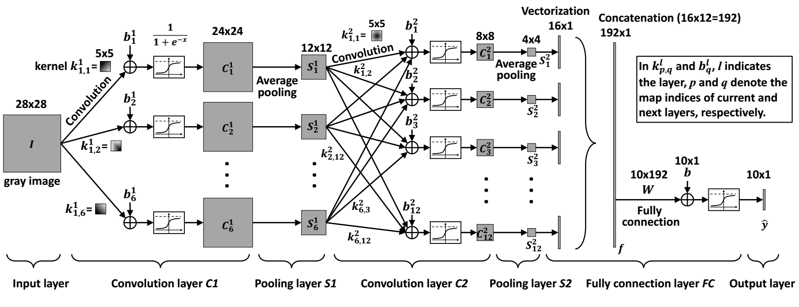
Figure 1. CNN for digit recognition. The picture is taken from (Zhang, 2016)

Figure 1 shows the construction of the network which starts from a $28\times 28$ pixel image of a digit and produces a 10-element $\hat{y}$ through a sequence of convolution and pooling layers. The vector $\hat{y}$ contains the probabilities of the input actually depicting the digits 0–9.

Convolution

In the first layer $C_{1}$, we compute six convolutions of the input image $I$ with $5\times 5$ matrices of weights $k^{1}_{1,i}$ producing six $24\times 24$ arrays. One such convolution can be implemented as:

⬇

float[*] conv(float[*] I, float[*] k) {

return { iv -> sum({ ov -> I[iv+ov] * k[ov]

| ov < shape(k) })

| iv < shape(I) - shape(k) + 1 };

}

The type float[*] denotes an array of floating point numbers of arbitrary shape. For our image $I$ of shape $[28,28]$ and any of the weights $k^{1}_{1,i}$ of shape $[5,5]$, the result is of shape $[28,28]-[5,5]+1=[24,24]$. Each element at the index position iv is computed as a sum of $5\times 5$ elements in I multiplied with the corresponding weights in k.

Using conv we can define a function mconv to compute the six convolutions and to add the individual biases $b^{1}_{i}$ to each convolution (denoted as $\oplus$ in Figure 1):

⬇

float[*] mconv(float[*] I, float[*] k, float[*] b) {

return { i -> conv(I, k[i]) + b[i]

| i < shape(b)};

}

This function is rank-polymorphic, and in the context of the $C_{1}$ layer we chose to store all $k$s in a 3D array of shape $[6,5,5]$. One bias per convolution leads to the shape of b being $[6]$. For every index in b, mconv computes the convolution of $I$ with k[ i ] that is adjusted by adding the b[ i ] bias. The expression k[ i ] selects a $[5,5]$ sub-array at the corresponding index, and ‘+ b[ i ]’ adds the scalar to every element of the $[24,24]$ array, resulting in the overall shape $[6,24,24]$.

The last step in $C_{1}$ is the application of the sigmoid activation function to all values. We define it with the overloaded versions of mathematical functions provided in the standard library of SaC:

⬇

float[*] sigmoid (float[*] in) {

return 1f / (1f + exp(-in));

}

This is a rank-polymorphic shape-preserving function, so its application to the result of mconv of shape $[6,24,24]$ yields the desired result of the same shape.

Consider now the convolution layer $C_{2}$. If we choose to represent $s$ as a 3D array of shape $[6,12,12]$, our rank-polymorphic specification of mconv becomes immediately applicable here. Intuitively, if $s$ is a single object, then all the left hand sides of the arrows from $S_{1}$ to $C_{2}$ in Figure 1 will merge into a single point, similarly to the first convolution. Our new input to conv is of shape $[6,12,12]$, so each $s^{i}$ should be of shape $[6,5,5]$, producing a result of shape $[1,8,8]$. As we have 12 $s^{i}$ and 12 biases, the application of the mconv would be of shape $[12,1,8,8]$. Note that the second element in the shape can be eradicated by a simple reshape, which does not alter the data representation in memory or its computational efficiency.

Applying the same reasoning to the $FC$ layer, we conclude that we can use mconv again. Without additional reshapes, the shape of the layer $S_{2}$ would be $[12,1,4,4]$. A fully connected layer is a convolution with the weight that is identical to the shape of the input array. Therefore, as we intend to compute ten weighted sums of all the elements, $W$ now has shape of $[10,12,1,4,4]$. This yields mconv to return a result of shape $[10,1,1,1,1]$. With these observations it becomes clear that the only parts of Figure 1 left to complete the implementation are the pooling layers.

Average Pooling

The pooling layer $S_{1}$ can be constructed in a two step process similarly to the convolution layers. An average pooling of a single image can be implemented as:

⬇

float[.,.] avgpool(float[.,.] in) {

return { iv -> average({ ov -> in[iv*2+ov]

| ov < [2,2] })

| iv < shape(in) / 2 };

}

We select sub-arrays of shape $[2,2]$ and compute their individual average, resulting in a matrix of half as many rows and columns as the input. Based on this definition, a generic version that applies avgpool to the two innermost axes of an $n$-dimensional array can be expressed as:

⬇

float[*] avgpool(float[*] in) {

return { iv -> avgpool(in[iv])

| iv < drop([-2], shape(in)) };

}

Note that for convenience we overload the name avgpool. With these few functions, we are now ready to define the whole network from Figure 1 as

⬇

float[10,1,1,1,1] forward(

float[28,28] I,

float[6,5,5] k1, float[6] b1,

float[12,6,5,5] k2, float[12] b2,

float[10,12,1,4,4] fc, float[10] b) {

c1 = sigmoid(mconv(I, k1, b1));

s1 = avgpool(c1);

c2 = sigmoid(mconv(s1, k2, b2));

s2 = avgpool(c2);

return sigmoid(mconv(s2, fc, b));

}

Explicit shapes in forward are given for documentation purposes, and they can be replaced with more generic shapes in case of more abstract networks.

The implementation so far suffices for using the network in forward mode, once suitable weights and biases are known, we can classify images. To adjust the weights, we use training inputs where we know the correct answer for every input image. The error in recognition is our cost function that we minimise by using stochastic gradient descent to adjust the weights.

Backpropagating Convolution

Our loss function has a form $\frac{1}{2}\sum{(y-f(x,w))}^{2}$, so its derivatives for $w_{i}$ will have a form $\frac{\partial f}{\partial w_{i}}f(x,w)\sum y-f(x,w)$ according to the chain rule. That is, to adjust the weights, we multiply the error with the derivative of the network with respect to the weights. The linear nature of the convolution implies that the derivatives are constants, namely the input of the convolution itself. Consequently, we can approximate the error in the weights as a convolution of the input with the error:

⬇

float[*] backweights(float[*] d_out, float[*] in) {

return conv(in, d_out);

}

The resulting deltas then can be used to adjust the corresponding weights for the next forward run. To cater for the imprecision, this is done by applying a factor, usually referred-to as rate.

⬇

...

weights = weights - rate*backweights(d_out,in);

...

Similarly, we can approximate the error of the bias as a sum of the error since the derivative of the bias is constant 1:

⬇

float[*] backbias(float[*] d_out) {

return sum(d_out);

}

The trickiest bit of implementation is the propagation of the error back to the inputs of the convolution, which we need to feed into the computation of the next backpropagation layer. Mathematically, the derivatives are simply the weights. The challenge arises from the fact that the outer elements of the result are influenced by fewer weights than the inner elements. This distinction between inner elements and outer elements can either be expressed by embedding the values of the array of errors into a larger array of zeros or it requires the summations for the boundary elements to range over fewer products. Here, we opt for the later approach:

⬇

float[*] backin(float[*] d_out,

float[*] k, float[*] in) {

return {

iv -> off = where(iv<shape(d_out),

0*shape(k),

iv-shape(d_out)+1);

sum({ ov -> k[ov+off]

* d_out[iv-(ov+off)]

| ov < min(min(shape(k), iv+1),

shape(k)-off) })

| iv < shape(in)

};

}

While all inner elements of the result are computed by k[ov] * d_out[iv-iv] with ov ranging over the entire shape of the weights k, the boundary elements are only computed using those factors where iv-ov lies within the shape of d_out. For the boundary elements on the lower end it suffices to restrict the number of products that are being summed up. This is achieved by the expression min(shape(k), iv+1). For the elements on the higher end, we only include the products with the higher-indexed weights. This is achieved by computing an offset vector off. For each index iv beyond the shape of the error in d_out, the offset is set accordingly. This is implemented by using the standard function where(m, b, c) which for each iv chooses b[ iv ] if m[ iv ] is true and c[ iv ] otherwise. Finally, we use this offset vector in order to restrict the number of products for the upper boundaries as well. This is achieved by the outer minimum against shape(k)-off.

Backpropagating Average Pooling

Average Pooling usually is back-propagated by evenly spreading out the error across the indices that we have averaged across in the forward mode. In our example, we can express this as:

⬇

float[.,.] backavgpool(float[.,.] d_out) {

return { iv -> d_out[iv/2] / 4f

| iv < shape(d_out) * 2 };

}

float[*] backavgpool(float[*] d_out) {

return { iv -> backavgpool(d_out[iv])

| iv < drop([-2], shape(d_out)) };

}

With these main building blocks, the back-propagation can be implemented in a way very similar to that of the forward function shown above. Details can be found at https://github.com/SacBase/CNN.

4. Evaluation

(a) Speedups (higher is better) over the fastest sequential runtime TF-Cxx-MKL.

(b) Wallclock Runtimes (lower is better).

Figure 2. CPU only results for SaC versus TensorFlow and PyTorch implementations using up to 64 Opteron cores, training 10 epochs on 10k images and classifying 10k images.

We now present an evaluation of our CNN implementations in SaC, comparing it to semantically identical implementations in TensorFlow and PyTorch. We discuss programming productivity reflecting our implementation experience, then we present our experimantal setup for runtime evaluation and we present performance analisys of the implementations.

4.1. Effect on Programming Productivity

Programmer productivity is a very personalised topic as the background in tool familiarity influences the experience. The tools that we are comparing are of a different nature: SaC is a general-purpose language, whereas TensorFlow and PyTorch are specifically designed for machine learning purposes, both highly performance-tuned and optimised for algorithms like the CNN. Neither of these tools executes the specification directly. Instead, the specification is analysed and translated into code that executes on parallel architectures.

All three specifications of the CNN in SaC, TensorFlow and PyTorch are very similar. In all systems about 150 lines of code are needed to specify the network and to orchestrate the reading of inputs and data initialisation. In all three versions, the programmer needs to understand the abstractions used; in TensorFlow and PyTorch, the programmer needs to learn semantics of the available components; in SaC, the programmer needs to understand the building blocks that we described in section 2. In SaC the backward propagation needs to be specified explicitly, while the frameworks tools support automatic differentiation.

Further experience is based on the fact that we also had to write the building blocks in SaC, if we assume that the machine learning framework is provided as an external tool then the next paragraph is not relevant. Otherwise, we found the conciseness of the building blocks very satisfying. The key components of which are described in section 3 can be implemented in about 150 lines of code. For someone with reasonable familiarity in SaC, this can be achieved within a few hours, depending on the familiarity with the underlying algorithm. Overall, the time we spent on the SaC implementation was considerably smaller than the time we needed to understand sufficient details about the TensorFlow and PyTorch frameworks. Of course this experience is hard to generalise, but we are rather sure that in cases where the hardware architecture and the machine learning algorithm is fixed, figuring out the details about the frameworks and implementing the algorithm from scratch is very likely to take comparable time.

4.2. Setup

Our machine is equipped with 4 AMD Opteron 6376 CPUs (for a total of 64 cores) and an NVIDIA K20 GPU (CUDA driver version 410.79). We use GCC 7.2.0, sac2c 1.3.3, CUDA 10.0, Python 3.6.6, TensorFlow 1.12.0 and PyTorch 1.2.0 for all applications.

We compile both frameworks from sources to make sure that the architecture specific flags like -march=native -mtune=native are passed to the C/C++ compilers so that we get proper vectorisation and cost models. Secondly, TensorFlow and PyTorch can make use of the Intel MKL library (Intel, 2009) to accelerate linear algebra operations on Intel architectures and provide a significant speedup. It is not compiled in by default for TensorFlow, and though we could make our comparison without it, it would not be an honest comparison. Therefore we have verified that MKL is correctly included in both frameworks, which has made a noticeable runtime difference. To make a fair comparison, we use a TensorFlow with and without Intel MKL (Intel, 2009) activated (indicated by the -MKL postfix), and we implement the CNN using both the Python and C++ interface (indicated by the Cxx postfix). The latter is to check whether static compilation has an impact on performance. This gives us five framework-based implementations, plus the on in SaC. We run these on both the CPU and GPU, and measure the wall-clock runtime of the entire application.

With non-MKL TensorFlow versions we set the number of threads via the session variables; for the MKL version, as the library uses OpenMP, setting the TensorFlow threads at the sametime can quickly oversubscribe the system, so per our experiments the best TensorFlow-MKL runtime is achieved when TensorFlow threads are set to 1 and the OMP_NUM_THREADS is set to the desirable value. With SaC we control the number of threads by setting the -mt flag of the binary file, that is automatically created by the compiler when using the multi-threaded backend.

The applications are run using the following parameters: 10 epochs, 100 images batch size, 10000 training images and labels, and 10000 test images and labels. The back-propagation has a learning rate factor of 0.05, and we do not use any momentum.

4.3. Results and Analysis

Figure 2(a) shows speedup compared to the fastest sequential runtime and 2(b) shows the runtimes in seconds. From 2(b) we can see that SaC outperforms all the other frameworks by a noticeable factor ($3\times$ over the best parallel runtime, $6\times$ over the best sequential runtime), even though being noticeably slower on a single thread. From 2(a) we see that none of the frameworks manage to achieve more than a $2\times$ speedup. We observe that TensorFlow applications using MKL are up to $2\times$ faster. Additionally, using the C++ over the Python interface is faster by a constant factor.

Table 1. Best wallclock runtimes (seconds) on the given hardware for each framework.

Framework	SaC	TF-Py	TF-Py-MKL	TF-Cxx	TF-Cxx-MKL	PT-Py-MKL
Configuration	Opteron 50 threads	NVIDIA K20	NVIDIA K20	NVIDIA K20	NVIDIA K20	NVIDIA K20
Runtime	7.8	17.06	18.26	17.68	14.1	24.32

The measurements in 2(a) show that for 10 threads we have speedups of up to a factor of 2 for the MKL-based applications, with the Python and C++ only applications achieving a speedup factor of about 1.5. The SaC application has a speedup factor of close to 3. As the number of threads increases, we see only minor improvements in speedup for the TensorFlow and PyTorch applications, with a best speedup factor of 2.3. The SaC application on the other hand continues to scale, reaching a max speedup factor of 6.4 using 50 threads. From 2(b) we can see this runtime plateauing more clearly. With MKL the runtimes are better than without for the TensorFlow and PyTorch applications, by almost a factor of 2. Additionally, using C++ instead of Python provides slightly better runtimes. We additionally re-ran the CNN using different batch-sizes and observered no significant change in the the previously observered scaling.

The speedup plateauing that we see for the TensorFlow and PyTorch applications relates to how nodes within the network graph are translated to threads. Some nodes have dependencies on outputs of others, and so are scheduled differently to nodes that have no dependencies. This limits the degree to which work can be distributed across the threads, affecting the max amount of scaling possible. Changes to the design of the network, or using a completely different neural-network can lead to different degrees of scaling. As SaC only translates with-loops to threads, and with-loops are guaranteed to be side-effect free, this leads to better scaling.

With TensorFlow we have two levels of parallelism, as the MKL operations spawn their own threads independently of the TensorFlow scheduler. We tried different combinations of threading configurations looking for the best possible performance. Using the default configuration, where TensorFlow and MKL use all cores, leads to oversubscription and degraded performance. Using combinations of values that match the number of logical cores on the system, such as 16 MKL threads and 4 TensorFlow threads, did not lead to better performance compared to just setting TensorFlow thread number to 1 and having MKL scale to all 64 logical cores. In any case we were not able to resolve the scaling plateau by this means.

Table 1 shows the best runtimes per application and the hardware configuration this was achieved on. The best runtime for SaC is 7.8 seconds using 50 threads. All other applications have their best runtime on the GPU, with the TensorFlow C++ MKL implementation having the best runtime at 14.01 seconds. The SaC application did not perform well on the GPU compared to the other applications, running $9\times$ slower.

A significant reason for this is the scheduling of communication and also kernel launches, that are not effectively orchestrated together. For TensorFlow and PyTorch, multiple CUDA streams are used to interleave communication and kernel launches such that they achieve a high degree of latency hiding.

4.4. Source of Performance in SaC

The SaC compiler is pretty sophisticated, it uses several hundred optimisations that run in a cycle, therefore explaining what exactly the compiler is doing to make the code run well is challenging. It would be good though to identify the key components, in order to potentially apply the demonstrated capabilities in other contexts, such as more mainstream function languages.

After looking at intermediate states of the code, we identify the following necessary optimisations: folding (Scholz, 1998), fusion (Grelck et al., 2006), memory reuse (Grelck and Trojahner, 2004), and statically-scheduled multi-threaded execution (Grelck, 2005).

Folding

The main idea behind folding is the classical list equality $\textit{map}\ f\circ\textit{map}\ g=\textit{map}\ f\circ g$, which can the eliminate creation of intermediate arrays. In the set notation this equality looks like:

⬇

a = {iv -> g | iv < u};

b = {iv -> $\lambda$iv.f a[$K$ iv] | iv < u}

$\Rightarrow$  ⬇ b = {iv -> $\lambda$iv.f (g ($K^{-1}$ iv)) | iv < u}

when $K=\text{identity}$, we get exactly the above equality. However, very often $K$s have computable inverses in which case the transformation is applicable to a larger set of examples. For the CNN case, we can definitely merge together the addition of biases and the computation of sigmoid functions in layers $C_{1}$, $C_{2}$ and $FC$.

Fusion

Here we apply a variant of the classical loop optimisation to array comprehensions. The optimisation combines the body of two consequent loops with an identical iteration space. In the map-based analogy this would be:

$$(\textit{map}\ f\ a,\textit{map}\ g\ a)=\textit{unzip}\ (\textit{map}\ f\Delta\,g\ a)$$

$$\text{where}\qquad{}(f\Delta\,g)\ x=(f\ x,g\ x)$$

Even though intuitively, this transformation does not make much sense on lists, it helps to localize the applications of $f$ and $g$ and share commons subexpressions. In SaC this optimisation is quite a bit more sophisticated, as explicit indexing makes it possible to define fusions on individual partitions of the index-spaces.

Memory Reuse

This memory analysis makes it possible to do array operations in-place. For example, when we increment all the elements by a constant:

$$b=\{\,iv\;\text{->}\;a[iv]+1\;|\linebreak\;iv\;\text{<}\;\texttt{shape}\,(a)\,\}$$

we can avoid allocating new memory, and reuse $a$, if $a$ is not used further in the program. The analysis becomes challenging when we consider reusing existing, but no longer referenced, arrays within the current scope. The analysis needs to handle conditionals within the set expression or the access patterns of candidate arrays.

Statically-Scheduled Parallelism

Finally, our array comprehensions are data parallel by design. Therefore, it is relatively straight forward to generate the code that partitions the index space into chunks and runs each chunk in parallel. Unfortunately, there is a lot of small details that makes it very hard to implement this efficiently (Gordon and Scholz, 2015). First of all, one needs to choose the operations we want to run in parallel, and their granularity. Secondly, choosing a schedule even for a single array operation is challenging. Finally, thread synchronisation and memory management make a significant difference. By default we use static scheduling, a custom memory allocator and for each operation we decide to run in parallel we try to choose the chunking that maximises the work each active thread is doing.

5. Related Work

5.1. Array Languages

Directly or indirectly, APL (Iverson, 1962) has influenced all existing array languages. At its core, APL provides a set of operators with a number of rules on how they can be composed. All operators are either unary or binary, first- or second-order functions, expressed with a single symbol, which gives a lot of expressiveness. For example, all the building blocks of our CNN can be expressed in 10 lines of code (Šinkarovs et al., 2019). APL is an untyped language, so all errors will occur at runtime only. It comes only with an interpreter and all the operators are implemented as library functions, limiting cross-operator optimisations.

Other array languages can be roughly divided into three groups: direct descendants of APL, grandchildren and further relatives. Direct descendants are languages like: J (Stokes, 2015), K (Whitney, 2001) or Nial (McCrosky et al., 1984). They treat every object as an array (maybe except functions) and provide a large subset of APL operators. Typically, these languages come only with interpreters, which limits the optimisations space and performance. The grandchildren like SaC, Futhark (Henriksen et al., 2017), Remora (Slepak et al., 2014), Qube (Trojahner and Grelck, 2009) are still array-oriented languages, but instead of providing built-in APL operators natively, they offer a few low-level constructs from which the operators could be implemented as library functions. All the mentioned languages are functional and come with compilers that are focused on generating high-performance code. All these languages have strong static type systems. Futhark and SaC are capable of generating GPU code automatically. Finally, further relatives like Matlab (The Mathworks, Inc., Natick, MA, 1992), Julia (Bezanson et al., 2017), Python (van Rossum, 1995) with Numpy (Oliphant, 2006) have some notion of multi-dimensional arrays and a subset of APL operators, both of which are embedded in the context of the general purpose language. All the mentioned languages come with interpreters only and rarely provide exceptional levels of performance, yet they are very useful for prototyping.

5.2. Machine learning DSLs

Machine Learning DSLs provide a way to express neural-networks using high-level specifications. Typically, the high-level specification is either handled by a machine learning framework, or transformed into machine code for performance reasons.

TypedFlow is embedded in Haskell and provides a number of dependently-typed primitives that can be used to define a network. Later this specification is translated into TensorFlow calls. This approach provides type safety, powerful syntax, but performance-wise, it sill relies on the underlying framework. The tensorflow-ocaml and ocaml-torch are similar wrappers for TensorFlow and PyTorch in Ocaml.

DEFIne (Dethlefs and Hawick, 2017) mainly focuses on liberating data scientists from the necessity to deal with general-purpose languages, such as Python, when describing the networks. The proposed syntax focuses exclusively on the machine learning primitives, and the accompanying tools take care of performance and portability, still using state of the art machine learning frameworks as a backend.

DeepDSL (Zhao and Huang, 2018), OptiML (Sujeeth et al., 2011) and Latte (Truong et al., 2016) focus on optimisations that are specific to machine learning such as kernel-fusion and parallelisation. They generate code to C++ and CUDA, using highly-optimised libraries.

The XLA (Google, 2017) is a domain-specific compiler that focuses on accelerating linear algebra operations in machine-learning applications. The compiler is a part of the TensorFlow framework, and it works by analysing dataflow graph of the network and turning it into fast machine code by fusing pipelined nodes, inferring tensor shapes and performing memory optimisations based on these data sizes.

Tensor Comprehensions (Vasilache et al., 2018) has a very similar idea: it is a DSL that is integrated into existing machine learning frameworks and it provides a common ground to implement machine learning operators for further cross-optimisation. A distinctive feature for this approach is the use of the polyhedral model to perform the actual fusion, blocking, non-trivial scheduling and parallelisation. In a way the approach is very similar to Halide (Ragan-Kelley et al., 2013), except the domain is different and the number of optimisations is larger.

Diesel (Elango et al., 2018) is a standalone DSL from NVIDIA that also relies on polyhedral framework to perform cross-operator optimisations and generate code for CUDA.

5.3. High-Performance Libraries

Most of the machine learning frameworks rely on highly-optimised libraries that implement tensor or linear algebra operations. The Eigen (Guennebaud et al., 2010) and Aten provide basic tensor operation and are being used by TensorFlow and PyTorch correspondingly. The MKL (Intel, 2009) and OpenBlas (OpenBlas, 2012) implement high-performance Basic Linear Aalebra Subrtoutines (BLAS) for CPUs. ATLAS (Whaley and Dongarra, 1998), BTO (Belter et al., 2009) and SPIRAL (Püschel et al., 2004) use automatic tuning to obtain the most efficient implementation of commonly used numerical algorithms on a chosen architecture. BLAS operations on CUDA are provided by CUBLAS (Nvidia, 2016). cuDNN (Chetlur et al., 2014) implements basic deep learning operations on GPUs. NNPACK and PCL-DNN (Das et al., 2016) implement deep learning primitives on CPUs.

6. Conclusions

This paper makes an argument for an alternative design of machine learning frameworks. Instead of using a large number of interconnected specialised libraries, we consider using one compilable array-oriented language to host both the framework and the specification of the actual networks. To justify the viability of the proposed approach, we implement a minimalistic framework in native SaC and use it to define a state of the art CNN. We compare its performance and expressiveness against TensorFlow and PyTorch.

Our solution is concise: about a 150 lines of code to define the building blocks of the network, and another 150 lines to define the network itself — which is about the same amount as for the TensorFlow and PyTorch versions. The basic building blocks in SaC are rank-polymorphic functions that can be easily reused in other contexts. Rank polymorphism is a key to expressiveness here. By the nature of layered neural networks, the notion of proximity arises naturally in multiple dimensions: neighbourhood of pixels, neighbouring neurons, connectivity between layers, convolutional weights, etc. In our simple example with 3 layers of neurons ($C_{1}$, $C_{2}$ and $FC$ from Fig. 1), we ended up with a single definition for multi-dimensional convolution which could serve all three layers with their varying ranks (3,4, and 5). The rank-polymorphic nature allows for arbitrarily ranked tensors and thus can be used for arbitrarily nested networks. The same holds for the other operations such as the backward propagation.

Our performance experiments on a 64-core machine with a GPU show that the SaC implementation outperforms TensorFlow and PyTorch by a factor of 2 and 3 respectively, even though the chosen architecture should be ideally suitable for both frameworks. In particular the performance results came as a big surprise to us, given the stark difference in implementation efforts. As discussed in Section 4, it seems that the interplay of different tools in TensorFlow and PyTorch are getting into the way of achieving excellent parallel performance, whereas the lean design in the array language setup enables better optimisations and ultimately better wallclock runtimes.

When shifting from the domain-specific frameworks to array-oriented languages we loose the domain-knowledge for optimisation on the one hand while we gain a unified high-level representation on the other. At least for the example of CNNs, it seems that the former does not provide any advantages for the frameworks whereas the latter clearly benefits the array language approach. Also, a unifying representation makes it very easy to extend a framework. There is no need to understand complexities of the udnerlying design — a new building block in the form of a user defined function will be immediately picked up by a compiler and included in the global program optimisations.

As for productivity and expressiveness, there is no doubt that right now Python is more advanced than any of the existing array languages, at least in the number of libraries provided by the community. At the same time, there seem to be no conceptual problem in bringing the same experience and functionality to the array language of choice. In the case of SaC two immediate problems will have to be solved: interactive behaviour and automatic differentiation.

Right now SaC is a compiled language and by default we do not get the same interactivity as with Python in the context of existing machine learning frameworks. However, right now there exists a jupyter-based frontend that mimics Python-like interactivity. Several other array languages are more interactive than SaC, and creating an interpreter for SaC is straight-forward. One then can envision using such an interpreter for quick prototyping and a compiled version of the same code for deployment.

Right now SaC does not support automatic differentiation which is a very useful feature that can be found in most of the machine learning frameworks. Adding automatic differentiation to a compiler is a well-understood problem as for example demonstrated by Stalin$\nabla$ (Pearlmutter and Siskind, 2008), therefore bringing it to the context of an array language is a matter of implementation effort.

By no means do we suggest that existing frameworks can be readily replaced by array languages. However, a clean design that eliminates a number of abstraction layers, supported by the fact that a prototypical research compiler can significantly outperform two industrial frameworks suggests that the proposed approach is interesting enough to be further investigated.

References

- (1)
- Abadi et al. (2016) Martín Abadi, Paul Barham, Jianmin Chen, Zhifeng Chen, Andy Davis, Jeffrey Dean, Matthieu Devin, Sanjay Ghemawat, Geoffrey Irving, Michael Isard, Manjunath Kudlur, Josh Levenberg, Rajat Monga, Sherry Moore, Derek G. Murray, Benoit Steiner, Paul Tucker, Vijay Vasudevan, Pete Warden, Martin Wicke, Yuan Yu, and Xiaoqiang Zheng. 2016. TensorFlow: A System for Large-Scale Machine Learning. In 12th USENIX Symposium on Operating Systems Design and Implementation (OSDI 16). USENIX Association, Savannah, GA, 265–283. https://www.usenix.org/conference/osdi16/technical-sessions/presentation/abadi
- Belter et al. (2009) Geoffrey Belter, E. R. Jessup, Ian Karlin, and Jeremy G. Siek. 2009. Automating the Generation of Composed Linear Algebra Kernels. In Proceedings of the Conference on High Performance Computing Networking, Storage and Analysis (SC ’09). ACM, New York, NY, USA, Article 59, 12 pages. https://doi.org/10.1145/1654059.1654119
- Bernecky (1997) Robert Bernecky. 1997. An Overview of the APEX Compiler. Technical Report 305/97. Department of Computer Science, University of Toronto.
- Bezanson et al. (2017) Jeff Bezanson, Alan Edelman, Stefan Karpinski, and Viral B. Shah. 2017. Julia: A Fresh Approach to Numerical Computing. SIAM Rev. 59, 1 (2017), 65–98. https://doi.org/10.1137/141000671
- Cann and Feo (1990) David Cann and John Feo. 1990. SISAL Versus FORTRAN: A Comparison Using the Livermore Loops. In Proceedings of the 1990 ACM/IEEE Conference on Supercomputing (Supercomputing ’90). IEEE Computer Society Press, Los Alamitos, CA, USA, 626–636. http://dl.acm.org/citation.cfm?id=110382.110593
- Chetlur et al. (2014) Sharan Chetlur, Cliff Woolley, Philippe Vandermersch, Jonathan Cohen, John Tran, Bryan Catanzaro, and Evan Shelhamer. 2014. cuDNN: Efficient Primitives for Deep Learning. CoRR abs/1410.0759 (2014). arXiv:1410.0759 http://arxiv.org/abs/1410.0759
- Collobert et al. (2011) Ronan Collobert, Koray Kavukcuoglu, Clément Farabet, et al. 2011. Torch7: A matlab-like environment for machine learning. In BigLearn, NIPS workshop, Vol. 5. Granada, 10.
- Das et al. (2016) Dipankar Das, Sasikanth Avancha, Dheevatsa Mudigere, Karthikeyan Vaidyanathan, Srinivas Sridharan, Dhiraj D. Kalamkar, Bharat Kaul, and Pradeep Dubey. 2016. Distributed Deep Learning Using Synchronous Stochastic Gradient Descent. CoRR abs/1602.06709 (2016). arXiv:1602.06709 http://arxiv.org/abs/1602.06709
- Dethlefs and Hawick (2017) Nina Dethlefs and Ken Hawick. 2017. DEFIne: A Fluent Interface DSL for Deep Learning Applications. In Proceedings of the 2nd International Workshop on Real World Domain Specific Languages (RWDSL17). ACM, New York, NY, USA, Article 3, 10 pages. https://doi.org/10.1145/3039895.3039898
- Elango et al. (2018) Venmugil Elango, Norm Rubin, Mahesh Ravishankar, Hariharan Sandanagobalane, and Vinod Grover. 2018. Diesel: DSL for Linear Algebra and Neural Net Computations on GPUs. In Proceedings of the 2Nd ACM SIGPLAN International Workshop on Machine Learning and Programming Languages (MAPL 2018). ACM, New York, NY, USA, 42–51. https://doi.org/10.1145/3211346.3211354
- Gauss (1809) Carl F. Gauss. 1809. Theoria motus corporum coelestium in sectionibus conicis solem ambientium. sumtibus F. Perthes et I. H. Besser. https://books.google.co.uk/books?id=ORUOAAAAQAAJ
- Google (2017) Google. 2017. https://www.tensorflow.org/xla/overview. [Accessed 2019/02].
- Gordon and Scholz (2015) Stuart Gordon and Sven-Bodo Scholz. 2015. Dynamic Adaptation of Functional Runtime Systems Through External Control. In Proceedings of the 27th Symposium on the Implementation and Application of Functional Programming Languages (IFL ’15). ACM, New York, NY, USA, Article 10, 13 pages. https://doi.org/10.1145/2897336.2897347
- Grelck (2005) Clemens Grelck. 2005. Shared Memory Multiprocessor Support for Functional Array Processing in Sac. Journal of Functional Programming 15, 3 (2005), 353–401. https://doi.org/10.1017/S0956796805005538
- Grelck et al. (2006) Clemens Grelck, Karsten Hinckfuß, and Sven-Bodo Scholz. 2006. With-Loop Fusion for Data Locality and Parallelism. In Implementation and Application of Functional Languages, Andrew Butterfield, Clemens Grelck, and Frank Huch (Eds.). Springer Berlin Heidelberg, Berlin, Heidelberg, 178–195.
- Grelck and Scholz (2003) Clemens Grelck and Sven-Bodo Scholz. 2003. Axis Control in Sac. In Implementation of Functional Languages, 14th International Workshop (IFL’02), Madrid, Spain, Revised Selected Papers (Lecture Notes in Computer Science), Ricardo Peña and Thomas Arts (Eds.), Vol. 2670. Springer, 182–198. https://doi.org/10.1.1.540.8938
- Grelck and Trojahner (2004) Clemens Grelck and Kai Trojahner. 2004. Implicit Memory Management for SaC. In Implementation and Application of Functional Languages, 16th International Workshop, IFL’04, Clemens Grelck and Frank Huch (Eds.). University of Kiel, Institute of Computer Science and Applied Mathematics, 335–348. Technical Report 0408.
- Guennebaud et al. (2010) Gaël Guennebaud, Benoît Jacob, et al. 2010. Eigen v3. http://eigen.tuxfamily.org.
- Henriksen et al. (2017) Troels Henriksen, Niels GW Serup, Martin Elsman, Fritz Henglein, and Cosmin E Oancea. 2017. Futhark: purely functional GPU-programming with nested parallelism and in-place array updates. In Proceedings of the 38th ACM SIGPLAN Conference on Programming Language Design and Implementation. ACM, 556–571.
- Indolia et al. (2018) Sakshi Indolia, Anil Kumar Goswami, S.P. Mishra, and Pooja Asopa. 2018. Conceptual Understanding of Convolutional Neural Network- A Deep Learning Approach. Procedia Computer Science 132 (2018), 679 – 688. https://doi.org/10.1016/j.procs.2018.05.069 International Conference on Computational Intelligence and Data Science.
- Intel (2009) Intel. 2009. Intel Math Kernel Library. Reference Manual. Santa Clara, USA. ISBN 630813-054US.
- Iverson (1962) Kenneth E. Iverson. 1962. A Programming Language. John Wiley & Sons, Inc., New York, NY, USA.
- Jia et al. (2014) Yangqing Jia, Evan Shelhamer, Jeff Donahue, Sergey Karayev, Jonathan Long, Ross Girshick, Sergio Guadarrama, and Trevor Darrell. 2014. Caffe: Convolutional Architecture for Fast Feature Embedding. In Proceedings of the 22Nd ACM International Conference on Multimedia (MM ’14). ACM, New York, NY, USA, 675–678. https://doi.org/10.1145/2647868.2654889
- Legendre (1805) A.M. Legendre. 1805. Nouvelles méthodes pour la détermination des orbites des comètes. F. Didot. https://books.google.co.uk/books?id=FRcOAAAAQAAJ
- McCrosky et al. (1984) C. D. McCrosky, J. J. Glasgow, and M. A. Jenkins. 1984. Nial: A Candidate Language for Fifth Generation Computer Systems. In Proceedings of the 1984 Annual Conference of the ACM on The Fifth Generation Challenge (ACM ’84). ACM, New York, NY, USA, 157–166. https://doi.org/10.1145/800171.809618
- Nvidia (2016) Nvidia. 2016. CUBLAS Library User Guide (v8.0 ed.). Technical Report. nVidia. http://docs.nvidia.com/cublas/index.html
- Oliphant (2006) Travis Oliphant. 2006. NumPy: A guide to NumPy. http://www.numpy.org. [Accessed 2019/02].
- OpenBlas (2012) OpenBlas. 2012. OpenBLAS Home Page. http://www.openblas.net. [Accessed 2019/02].
- Paszke et al. (2017) Adam Paszke, Sam Gross, Soumith Chintala, Gregory Chanan, Edward Yang, Zachary DeVito, Zeming Lin, Alban Desmaison, Luca Antiga, and Adam Lerer. 2017. Automatic differentiation in PyTorch. In NIPS-W.
- Pearlmutter and Siskind (2008) Barak A. Pearlmutter and Jeffrey Mark Siskind. 2008. Reverse-mode AD in a Functional Framework: Lambda the Ultimate Backpropagator. ACM Trans. Program. Lang. Syst. 30, 2, Article 7 (March 2008), 36 pages. https://doi.org/10.1145/1330017.1330018
- Püschel et al. (2004) Markus Püschel, José M. F. Moura, Bryan Singer, Jianxin Xiong, Jeremy Johnson, David Padua, Manuela Veloso, and Robert W. Johnson. 2004. Spiral: A Generator for Platform-Adapted Libraries of Signal Processing Alogorithms. The International Journal of High Performance Computing Applications 18, 1 (2004), 21–45. https://doi.org/10.1177/1094342004041291 arXiv:https://doi.org/10.1177/1094342004041291
- Ragan-Kelley et al. (2013) Jonathan Ragan-Kelley, Connelly Barnes, Andrew Adams, Sylvain Paris, Frédo Durand, and Saman Amarasinghe. 2013. Halide: A Language and Compiler for Optimizing Parallelism, Locality, and Recomputation in Image Processing Pipelines. In Proceedings of the 34th ACM SIGPLAN Conference on Programming Language Design and Implementation (PLDI ’13). ACM, New York, NY, USA, 519–530. https://doi.org/10.1145/2491956.2462176
- Schmidhuber (2015) Jürgen Schmidhuber. 2015. Deep learning in neural networks: An overview. Neural Networks 61 (2015), 85 – 117. https://doi.org/10.1016/j.neunet.2014.09.003
- Scholz (1998) Sven-Bodo Scholz. 1998. With-loop-folding in Sac — Condensing Consecutive Array Operations. In Implementation of Functional Languages, 9th International Workshop (IFL’97), St. Andrews, UK, Selected Papers (Lecture Notes in Computer Science), Chris Clack, Tony Davie, and Kevin Hammond (Eds.), Vol. 1467. Springer, 72–92. https://doi.org/10.1007/BFb0055425
- Scholz (2003) Sven-Bodo Scholz. 2003. Single Assignment C: Efficient Support for High-level Array Operations in a Functional Setting. J. Funct. Program. 13, 6 (Nov. 2003), 1005–1059. https://doi.org/10.1017/S0956796802004458
- Slepak et al. (2014) Justin Slepak, Olin Shivers, and Panagiotis Manolios. 2014. An Array-Oriented Language with Static Rank Polymorphism. In Programming Languages and Systems, Zhong Shao (Ed.). Springer Berlin Heidelberg, Berlin, Heidelberg, 27–46.
- Steuwer et al. (2017) Michel Steuwer, Toomas Remmelg, and Christophe Dubach. 2017. Lift: a functional data-parallel IR for high-performance GPU code generation. In CGO. ACM, 74–85.
- Stokes (2015) Roger Stokes. 15 June 2015. Learning J. An Introduction to the J Programming Language. http://www.jsoftware.com/help/learning/contents.htm. [Accessed 2019/02].
- Sujeeth et al. (2011) Arvind K. Sujeeth, Hyoukjoong Lee, Kevin J. Brown, Hassan Chafi, Michael Wu, Anand R. Atreya, Kunle Olukotun, Tiark Rompf, and Martin Odersky. 2011. OptiML: an implicitly parallel domainspecific language for machine learning. In in Proceedings of the 28th International Conference on Machine Learning, ser. ICML.
- The Mathworks, Inc., Natick, MA (1992) The Mathworks, Inc., Natick, MA. 1992. MATLAB Reference Guide.
- Trojahner and Grelck (2009) Kai Trojahner and Clemens Grelck. 2009. Dependently typed array programs don’t go wrong. The Journal of Logic and Algebraic Programming 78, 7 (2009), 643 – 664. https://doi.org/10.1016/j.jlap.2009.03.002 The 19th Nordic Workshop on Programming Theory (NWPT 2007).
- Truong et al. (2016) Leonard Truong, Rajkishore Barik, Ehsan Totoni, Hai Liu, Chick Markley, Armando Fox, and Tatiana Shpeisman. 2016. Latte: A Language, Compiler, and Runtime for Elegant and Efficient Deep Neural Networks. In Proceedings of the 37th ACM SIGPLAN Conference on Programming Language Design and Implementation (PLDI ’16). ACM, New York, NY, USA, 209–223. https://doi.org/10.1145/2908080.2908105
- van Rossum (1995) G. van Rossum. 1995. Python tutorial. Technical Report CS-R9526. Centrum voor Wiskunde en Informatica (CWI), Amsterdam.
- Vasilache et al. (2018) Nicolas Vasilache, Oleksandr Zinenko, Theodoros Theodoridis, Priya Goyal, Zachary DeVito, William S. Moses, Sven Verdoolaege, Andrew Adams, and Albert Cohen. 2018. Tensor Comprehensions: Framework-Agnostic High-Performance Machine Learning Abstractions. CoRR abs/1802.04730 (2018). arXiv:1802.04730 http://arxiv.org/abs/1802.04730
- Šinkarovs et al. (2019) Artjoms Šinkarovs, Robert Bernecky, and Sven-Bodo Scholz. 2019. Convolutional Neural Networks in APL. In Proceedings of the 6th ACM SIGPLAN International Workshop on Libraries, Languages and Compilers for Array Programming (ARRAY 2019). ACM, New York, NY, USA, 69–79. https://doi.org/10.1145/3315454.3329960
- Whaley and Dongarra (1998) R. Clint Whaley and Jack J. Dongarra. 1998. Automatically Tuned Linear Algebra Software. In Proceedings of the 1998 ACM/IEEE Conference on Supercomputing (SC ’98). IEEE Computer Society, Washington, DC, USA, 1–27. http://dl.acm.org/citation.cfm?id=509058.509096
- Whitney (2001) Arthur Whitney. 2001. K. http://archive.vector.org.uk/art10010830.
- Yu et al. (2014) Dong Yu, Adam Eversole, Mike Seltzer, Kaisheng Yao, Zhiheng Huang, Brian Guenter, Oleksii Kuchaiev, Yu Zhang, Frank Seide, Huaming Wang, et al. 2014. An introduction to computational networks and the computational network toolkit. Microsoft Technical Report MSR-TR-2014–112 (2014).
- Zhang (2004) Tong Zhang. 2004. Solving Large Scale Linear Prediction Problems Using Stochastic Gradient Descent Algorithms. In Proceedings of the Twenty-first International Conference on Machine Learning (ICML ’04). ACM, New York, NY, USA, 116–. https://doi.org/10.1145/1015330.1015332
- Zhang (2016) Zhifei Zhang. 2016. Derivation of Backpropagation in Convolutional Neural Network (CNN). Technical Report. University of Tennessee, Knoxvill, TN. {http://web.eecs.utk.edu/~zzhang61/docs/reports/2016.10%20-%20Derivation%20of%20Backpropagation%20in%20Convolutional%20Neural%20Network%20(CNN).pdf}
- Zhao and Huang (2018) Tian Zhao and Xiaobing Huang. 2018. Design and implementation of DeepDSL: A DSL for deep learning. Computer Languages, Systems & Structures 54 (2018), 39 – 70. https://doi.org/10.1016/j.cl.2018.04.004