Multimodal Agglomeration in Economic Geography

Abstract

Multimodal agglomerations, in the form of the existence of many cities, dominate modern economic geography. We focus on the mechanism by which multimodal agglomerations realize endogenously. In a spatial model with agglomeration and dispersion forces, the spatial scale (local or global) of the dispersion force determines whether endogenous spatial distributions become multimodal. Multimodal patterns can emerge only under a global dispersion force, such as competition effects, which induce deviations to locations distant from an existing agglomeration and result in a separate agglomeration. A local dispersion force, such as the local scarcity of land, causes the flattening of existing agglomerations. The resulting spatial configuration is unimodal if such a force is the only source of dispersion. This view allows us to categorize extant models into three prototypical classes: those with only global, only local, and local and global dispersion forces. The taxonomy facilitates model choice depending on each study’s objective.

JEL: C62, R12, R13

Keywords: agglomeration; dispersion; economic geography; many regions; spatial scale

1 Introduction

The agglomeration of economic activities is a phenomenon that has been observed since humans shifted from nomadic to sedentary life after the advent of farming (Mumford-Book1961; Bairoch-Book1988). This tendency has continued throughout history, and urban agglomeration has become ubiquitous worldwide. The world’s urban population share increased from less than 30% in 1950 to 55% in 2018 and is forecast to reach 68% in 2050 (UN-WorldUrbanizationProspects2018). In many post-industrial economies such as France, Japan, the UK, and the US, this share has already exceeded 80%. Urban areas in these economies typically consist of many cities, indicating that modern economic geography is characterized by multimodal agglomeration.

Over the past decades, many theoretical models have been proposed to explain economic agglomeration through endogenous trade-offs between the costs and benefits of the spatial concentration of mobile actors (e.g., Fujita-Krugman-Venables-Book1999; Baldwin-et-al-Book2003; Duranton-Puga-HB2004; Fujita-Thisse-Book2013). However, in the context of many-region settings where multimodal agglomeration can emerge, they suffer from intractability owing to multiple equilibria, which has also been an obstacle for structural analyses (Redding-Rossi-Hansberg-ARE2017). To circumvent this difficulty, most recent studies either abstract from the geographical address of economic agglomerations by adopting the system-of-cities framework by Henderson-AER1974 (e.g., Behrens-et-al-JPE2014; Gaubert-AER2018; Duranton-Puga-DP2019; Davis-Dingel-JIE2020), or assume that negative effects of agglomeration dominate the positive ones to ensure the uniqueness of equilibrium as in the quantitative spatial economics (QSE) (e.g., Redding-Sturm-AER2008; Allen-Arkolakis-QJE2014; Caliendo-et-al-ECTA2019).

The former class of models explains large city-size diversity through endogenous agglomeration and dispersion forces. However, their stylized formulations without intercity distance do not allow us to address the spatial distribution of cities. In contrast, the latter class of models emphasizes the role of interregional transport costs. This literature focuses on counterfactual exercises assuming the uniqueness of equilibrium, as it “does not aim to provide a fundamental explanation for the agglomeration of economic activity” (Redding-Rossi-Hansberg-ARE2017, §1). However, the resulting comparative statics are inevitably model specific and could drastically differ depending on the chosen composition of endogenous forces. A systematic understanding of such model dependence is lacking. This state of literature calls for further investigations into the theoretical underpinnings of the agglomeration phenomena in many-region geography through endogenous mechanisms.

In this study, we contribute to developing a foundation of many-region quantitative spatial models that allow for multiple equilibria. We consider a general class of many-region models encompassing many extant models and reveal what combination of agglomeration and dispersion forces endogenously produces multimodal agglomeration in these models. In this respect, we regard the spatial scale of a dispersion force as local when the force arises from the interactions inside each region (e.g., urban costs owing to higher land rent or congestion in cities), and global when the force depends on the proximity structure between regions (e.g., competition effects between firms that may extend over a certain distance). We demonstrate that multimodal agglomeration emerges only when global dispersion forces are embedded in the model, irrespective of the nature of agglomeration forces. Models with only local dispersion force, such as first-generation regional QSE models (e.g., Redding-Sturm-AER2008; Allen-Arkolakis-QJE2014), in contrast, generate at most a unimodal (single-peaked) agglomeration.

Our analytical approach builds on Akamatsu-Takayama-Ikeda-JEDC2012 to impose a many-region racetrack economy (Papageorgiou-Smith-ECTA1983; krugman1993number) in which regions with the same characteristics are evenly located over a circumference. This setup abstract away exogenous asymmetry and allows us to focus on the role of endogenous economic forces. With the dichotomy between the local and global dispersion forces, we define three prototypical model classes that typical extant models fall into, regardless of their particular micro-foundations. A model is Class I (II) if only a global (local) dispersion force is at work and Class III if both local and global dispersion forces are at work (Table 1). Proposition 1 considers the endogenous spatial patterns that emerge upon the instability of the symmetric equilibrium, the uniform spatial distribution of agents across regions, and shows that they are distinctive for the model classes. A multimodal distribution (Figure 1A) can be obtained only when the model has a global dispersion force (Classes I or III), whereas a unimodal distribution (Figure 1B) is the only possibility when the model has only a local dispersion force (Class II).

	Class I	Class II	Class III
Global dispersion force	$\checkmark$		$\checkmark$
Local dispersion force		$\checkmark$	$\checkmark$
Examples	Harris-Wilson-EPA1978 Krugman-JPE1991 Puga-EER1999 (§3)	Beckmann-Book1976 Helpman-Book1998 Allen-Arkolakis-QJE2014	Tabuchi-JUE1998 Puga-EER1999 (§4) Pfluger-Suedekum-JUE2008

Table 1: Spatial scale of dispersion forces at work and model classes

A Multimodal agglomeration

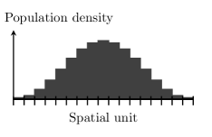
B Unimodal agglomeration

Figure 1: Spatial configurations in a one-dimensional economy

A simple thought experiment can illustrate the qualitative difference between the local and global dispersion forces and why the difference leads to different spatial patterns. Consider a many-region model with agglomeration forces. Without dispersion forces, all mobile agents would locate in one region. Mobile agents may deviate from this region if a dispersion force is added to the model. The spatial scale of the dispersion force affects the resulting spatial patterns in a many-region economy with heterogeneous interregional distances. Consider a local dispersion force, such as congestion within a region, for which the negative effect of concentration in a given region does not extend beyond the region. In this case, agents disperse locally as they can mitigate congestion by relocating to the adjacent regions, resulting in a unimodal pattern. A global dispersion force, such as competition between regions, affects all regions that are close to the agglomeration. In this case, agents (firms) must relocate to regions remote from the populated region to avoid the negative effect, resulting in multiple disjoint agglomerations.

Besides the difference in the spatial pattern of agglomeration, global and local dispersion forces respond oppositely to the change in transport costs. Better transport access fosters (discourages) agglomeration under a global (local) dispersion force. On the one hand, decreasing transport costs enable firms and consumers to reach more distant markets, enlarging firms’ market areas. Firms and consumers thus locate in fewer larger cities, leading to global concentration. On the other hand, lower transportation costs reduce the need for agents to locate close to each other and raise the relative importance of congestion effects. Consequently, each agglomeration experiences local dispersion in the form of a decrease in peak population density and an increase in area. In Class III models equipped with local and global dispersion forces, a reduction in transport costs simultaneously promotes global concentration and local dispersion.

The evolution of Japanese cities over the 50 years between 1970 and 2020 is an ideal example of global concentration and local dispersion. Transportation and communication costs plummeted in Japan during this period, as high-speed railway and highway networks were built across the country almost from scratch and the latter half of this period witnessed the spread of the Internet. Global concentration was observed during this period, as the number of cities decreased steadily. The cities that remained after the 50-year period experienced an average 46 % increase in population size (Fig. 2A). These cities also attracted substantial in-migration from across the country as the national population increased by only 21% during the same period.

Figure 2: Global concentration of population in Japan between 1970 and 2020

(A) The distribution of the ratio of the city sizes in 2020 to 1970 for the 314 cities that existed in both years. The growth in national population size is controlled by using each city’s share of the national population as its size. (B) The city size of each city-size rank in each year relative to that of the same city-size rank in 1970 for the largest 431 cities, which is the minimum number of cities during the period. Red lines indicate the top 100 cities, while blue ones illustrates the rest of the cities. The dashed line indicates the national population relative to the 1970 level.

Figure 2B shows the relative evolution of city sizes from 1970 to 2020. There is a clear tendency of concentration toward larger cities at the national (or global) level, as the sizes of the top 100 cities as of 2020 (red curves) and the rest of the cities (blue curves) diverged. However, within each city, there has been substantial local dispersion. On average, the cities that remained after the 50-year period experienced 34% and 23% decreases in peak and average population density, respectively, and an 88% increase in areal size (Fig. 3). The global concentration and local dispersion observed in the development of Japanese cities under diminishing transport costs are qualitatively consistent with the expected outcomes from Class III models.

Figure 3: Local dispersion within a city in Japan between 1970 and 2020

(A, B, C) The changes in the peak population density, average population density, and areal size in 2020 to those in 1970, respectively, of 314 cities that existed in both years.

Finally, we explore implications to the QSE literature by examining how the interplay between exogenous location-specific factors and endogenous agglomeration and dispersion forces influences comparative statics. A standard approach in QSE models is to impose parametric restrictions to ensure the uniqueness of equilibrium, suppressing endogenous agglomeration (Redding-Rossi-Hansberg-ARE2017, §3.9). We demonstrate that, under such a setting, the spatial scale of the dispersion force embedded in a model can govern the comparative statics of the model irrespective of its specific micro-foundations. Specifically, Proposition 2 provides a comparative static result on how endogenous agglomeration force augments or discourages exogenous regional advantages, crucial factors in quantitative models when transport costs change. Naturally, an exogenously advantageous region attracts a higher population than the average for a given transport cost level, other factors being equal. Suppose that inter-regional access improves. In Class I models with only global dispersion force, the exogenous advantage specific to a given region is magnified. The converse is true for Class II models with only local dispersion force (e.g., Allen-Arkolakis-QJE2014, Allen-Arkolakis-QJE2014, §III.C; Redding-Rossi-Hansberg-ARE2017, Redding-Rossi-Hansberg-ARE2017, §3.9). The resulting implications can thus be the opposite depending on the dispersion force to be embedded in the quantitative spatial models. A better transport connection between the core and periphery regions will leave the periphery behind the core under Class I models, while it will benefit the periphery under Class II models. That said, the knowledge of endogenous agglomeration mechanisms appears crucial in policy decisions based on quantitative models.

The remainder of this paper is organized as follows: Section 2 introduces the class of models we focus on; Section 3 defines the spatial scale of dispersion forces and the three prototype model classes; Section 4 presents Proposition 1; Section 5 explores the effects of exogenous asymmetries to provide Proposition 2; Section 6 concludes the paper. All the proofs are provided in Appendix B.

2 Basic framework

We consider generic many-region spatial models, which we call economic geography models. Definition 1 will introduce canonical models, the class of models we focus on.

2.1 Economic geography models

Consider an economy comprised of $N$ regions, where a “region” is an arbitrary discrete spatial unit. Let $\mathcal{N}\equiv\{1,2,\ldots,N\}$ be the set of regions. There is a continuum of agents, and each agent chooses a region that maximizes their utility. Let $\bm{x}\equiv(x_{i})_{i\in\mathcal{N}}$ be the spatial distribution of agents where $x_{i}\geq 0$ is the mass of agents in region $i$ with $\sum_{i\in\mathcal{N}}x_{i}=1$. The payoff of agents in region $i$ is summarized by the indirect utility function $v_{i}(\bm{x})$. We assume that $\bm{v}(\bm{x})\equiv(v_{i}(\bm{x}))_{i\in\mathcal{N}}$ is differentiable if $x_{i}>0$ for all $i\in\mathcal{N}$.

Agents can freely relocate across $N$ regions to improve their payoffs. Then, $\bm{x}$ is a spatial equilibrium if the following Nash equilibrium condition is met: $v^{*}=v_{i}(\bm{x})$ for any region $i\in\mathcal{N}$ with $x_{i}>0$, while $v^{*}\geq v_{i}(\bm{x})$ for all $i\in\mathcal{N}$ with $x_{i}=0$, with $v^{*}=\max_{i\in\mathcal{N}}\{v_{i}(\bm{x})\}$ being the associated equilibrium payoff level.

An indispensable feature of an economic geography model is the presence of spatial frictions for, for example, the shipment of goods or communication among agents. We suppose that $\bm{v}$ depends on a proximity matrix $\mathbf{D}=[\phi_{ij}]$ that summarizes interregional transport costs. Each entry $\phi_{ij}\in(0,1]$ is the freeness of interactions between regions $i$ and $j$ (e.g., freeness of trade, transportation, or social communication).

Indirect utility function $\bm{v}$ can include positive and negative externalities of spatial concentration, which may depend on interregional transport costs. Economic geography models often face multiple spatial equilibria because of the positive externalities. Following the literature, we use equilibrium refinement based on asymptotic stability under myopic dynamics (Fujita-Krugman-Venables-Book1999). We presume a class of dynamics that includes standard dynamics in the literature. All the formal claims on the stability of equilibria in this study hold for the dynamics listed in Example B.1 in Appendix B. For example, the class of dynamics includes the Brown–von Neumann–Nash dynamic (Brown-vonNeumann-Rand1950; Nash-AM1951), the Smith dynamic (Smith-TS1984), and the replicator dynamic (Taylor-Jorker-MB1978).

2.2 Symmetric racetrack economy

Figure 4: $N$-region racetrack economy.

We consider an $N$-region economy in which regions are symmetrically placed over a circle and interactions are possible only along the circumference (Figure 4).

Assumption RE (Racetrack economy).

Proximity matrix $\mathbf{D}=[\phi_{ij}]$ is given by $\phi_{ij}=\phi^{\ell_{ij}}$, where $\phi\in(0,1)$ is the freeness of interactions between two consecutive regions and $\ell_{ij}\equiv\min\{|i-j|,N-|i-j|\}$ is the distance between regions $i$ and $j$ over the circumference. Further, $N$ is a multiple of four.

The assumption abstracts from the location-specific advantages induced by the shape of the transport network. For expositional simplicity, we assume $N$ is a multiple of four. Where the many-region economy is unnecessary for discussion, we use two-region examples.

In addition to asymmetries in transport accessibility, we abstract away all asymmetries in local regional characteristics to focus on endogenous factors. We assume that payoff function $\bm{v}$ does not introduce any ex-ante asymmetries across regions.

Assumption S (Symmetry of payoff function).

For all $\bm{x}$, payoff function $\bm{v}$ satisfies $\bm{v}(\mathbf{P}\bm{x})=\mathbf{P}\bm{v}(\bm{x})$ for all permutation matrices $\mathbf{P}$ with $\mathbf{P}\mathbf{D}=\mathbf{D}\mathbf{P}$.

The condition $\mathbf{P}\mathbf{D}=\mathbf{D}\mathbf{P}$ means that the adjacency relationships between regions remain invariant under the permutation of the regional indices represented by $\mathbf{P}$. For example, suppose $N=4$. Then, Assumption RE is that

$$\mathbf{D}=\begin{bmatrix}1&\phi&\phi^{2}&\phi\\ \phi&1&\phi&\phi^{2}\\ \phi^{2}&\phi&1&\phi\\ \phi&\phi^{2}&\phi&1\end{bmatrix}.$$ (1)

The geometry of the circular economy is invariant even if we swap the indices of regions $1$ and $3$. The following permutation matrix $\mathbf{P}$, which satisfies $\mathbf{P}\mathbf{D}=\mathbf{D}\mathbf{P}$, represents this re-indexing:

$$\mathbf{P}=\begin{bmatrix}&&1&\\ &1&&\\ 1&&&\\ &&&1\end{bmatrix}.$$ (2)

Given a spatial distribution $\bm{x}=(x_{1},x_{2},x_{3},x_{4})$, the re-indexed spatial distribution becomes $\bm{x}^{\prime}=(x_{3},x_{2},x_{1},x_{4})=\mathbf{P}\bm{x}$. If $\bm{v}$ does not include any region-specific exogenous advantages, it must be $v_{1}(\bm{x}^{\prime})=v_{3}(\bm{x})$, $v_{2}(\bm{x}^{\prime})=v_{2}(\bm{x})$, $v_{3}(\bm{x}^{\prime})=v_{1}(\bm{x})$, and $v_{4}(\bm{x}^{\prime})=v_{4}(\bm{x})$, that is, $\bm{v}(\bm{x}^{\prime})=\bm{v}(\mathbf{P}\bm{x})=\mathbf{P}\bm{v}(\bm{x})$.

Under Assumptions RE and S, the uniform distribution $\bar{\bm{x}}\equiv(\bar{x},\bar{x},\ldots,\bar{x})$ with $\bar{x}=\frac{1}{N}$ is always a spatial equilibrium. If $\bar{\bm{x}}$ is stable, the spatial distribution remains flat. If $\bar{\bm{x}}$ is unstable, it results in the formation of nontrivial spatial agglomeration (Papageorgiou-Smith-ECTA1983; Krugman-JPE1991). Below, we consider what spatial patterns emerge from $\bar{\bm{x}}$ when it becomes unstable.

2.3 Endogenous agglomeration in a two-region economy

We start with the two-region example for illustration. Suppose two regions have identical characteristics. The proximity matrix is

$$\mathbf{D}=\begin{bmatrix}1&\phi\\ \phi&1\end{bmatrix},$$ (3)

where $\phi\in(0,1)$ is the freeness of transport between the two regions. The uniform distribution of agents, $\bar{\bm{x}}\equiv\left(\bar{x},\bar{x}\right)$ with $\bar{x}=\frac{1}{2}$, is always a spatial equilibrium.

For the stability of $\bar{\bm{x}}$, there is a general model-independent characterization. The symmetric state $\bar{\bm{x}}$ is stable (unstable) if the payoff gain of an agent relocating from one region to the other is negative (positive). The gain for a deviant can be evaluated by the elasticity of the payoff difference:

$$\omega =\frac{\bar{x}}{\bar{v}}\dfrac{\partial{\left(v_{1}(\bar{\bm{x}})-v_{2}(\bar{\bm{x}})\right)}}{\partial{x_{1}}}=\frac{\bar{x}}{\bar{v}}\left(\dfrac{\partial{v_{1}(\bar{\bm{x}})}}{\partial{x_{1}}}-\dfrac{\partial{v_{2}(\bar{\bm{x}})}}{\partial{x_{1}}}\right),$$ (4)

where $\bar{v}$ is the uniform payoff level at $\bar{\bm{x}}$, so that $\bm{v}(\bar{\bm{x}})=(\bar{v},\bar{v})$.

If $\omega<0$, then a marginal increase in the mass of agents in a region induces a relative payoff decrease therein compared to the other region, and agents are worse off by such migration. Thus, $\bar{\bm{x}}$ is stable. In fact, $\omega<0$ implies that $\bar{\bm{x}}$ is an evolutionary stable states (Sandholm-Book2010, Observation 8.3.11). If $\omega>0$, the migration of a small fraction of agents from region $2$ to $1$ induces a relative payoff increase in region $1$ compared to region $2$. In this case, $\bar{\bm{x}}$ is unstable because agents are strictly better off when they migrate to the other region.

Suppose that $\bar{\bm{x}}$ is initially stable ($\omega<0$). If $\omega$ turns from negative to positive due to gradual changes in underlying conditions of the economy, then agents can improve their payoffs by migration, and endogenous regional asymmetry emerges. By construction, $\omega$ is a function of parameters of $\bm{v}$, including the freeness of interregional interactions $\phi$. Monotonic change in $\phi$ may thus switch the sign of $\omega$ from negative to positive, leading to endogenous agglomeration.

Let $\mathbf{V}\equiv\frac{\bar{x}}{\bar{v}}\nabla\bm{v}(\bar{\bm{x}})=\frac{\bar{x}}{\bar{v}}[\frac{\partial v_{i}}{\partial x_{j}}(\bar{\bm{x}})]$ be the matrix of payoff elasticity with respect to $\bm{x}$ evaluated at $\bm{x}=\bar{\bm{x}}$. Then, we can demonstrate that $\omega$ is an eigenvalue of $\mathbf{V}$ and its associated eigenvector is $\bm{z}\equiv(1,-1)$, i.e., $\mathbf{V}\bm{z}=\omega\bm{z}$. As $\bm{z}$ represents a population increase in one region and a decrease in the other, it is the migration pattern in the two-region economy. Evidently, $\bm{z}$ does not depend on details of $\bm{v}$ and is common for all models.

We provide a concrete example of endogenous agglomeration below.

Example 2.1 (The Beckmann model).

Beckmann-Book1976 proposed a seminal model for the formation of an urban center within a city. We use a discrete-space version to fit the model to our context instead of the original formulation in a continuous space. Consider the following specification:

$$v_{i}(\bm{x})=x_{i}^{-\gamma}E_{i}(\bm{x}).$$ (5)

The first component, $x_{i}^{-\gamma}$ with $\gamma>0$, represents negative externalities due to congestion. The second, $E_{i}(\bm{x})$, represents positive externalities of agglomeration. Each agent prefers proximity to other agents. A typical specification is

$$E_{i}(\bm{x})=\sum_{j\in\mathcal{N}}\mathrm{e}^{-\tau\ell_{ij}}x_{j},$$ (6)

where $\tau>0$ is the distance-decay parameter and $\ell_{ij}>0$ is the distance between $i$ and $j$. The proximity matrix for the model is $\mathbf{D}=[\mathrm{e}^{-\tau\ell_{ij}}]$. ∎

Suppose $N=2$. Then, $\phi=\mathrm{e}^{-\tau\ell_{12}}=\mathrm{e}^{-\tau\ell_{21}}\in(0,1)$ is the level of externalities from one location to the other. We have $\mathbf{V}=-\gamma\mathbf{I}+\bar{\mathbf{D}}$, where $\bar{\mathbf{D}}=\frac{1}{1+\phi}\mathbf{D}$ is the row-normalized version of $\mathbf{D}$ in (3).

The only possible migration direction, $\bm{z}=(1,-1)$, is an eigenvector of $\bar{\mathbf{D}}$ because it satisfies $\bar{\mathbf{D}}\bm{z}=\chi\bm{z}$ with

$$\chi=\frac{1-\phi}{1+\phi}\in(0,1).$$ (7)

We observe that $\chi$ is monotonically decreasing in $\phi\in(0,1)$. If $\phi$ is small (large), $\chi$ is large (small). We can interpret $\chi$ as an index of transport cost where the higher $\chi$ corresponds to the higher transport cost level (smaller $\phi$). With $\chi$, the relevant eigenvalue of $\mathbf{V}$ is given as $\omega=-\gamma+\chi$.

The negative term $-\gamma$ in $\omega$ corresponds to the congestion effect through $x_{i}^{-\gamma}$ in $v_{i}(\bm{x})$. The positive term $\chi$ corresponds to positive externalities $E_{i}(\bm{x})$. The former is the marginal loss from congestion, whereas the latter is the marginal gains from the proximity induced by deviation from $\bar{\bm{x}}$.

If $\gamma\geq 1$, then $\omega<0$ for all $\phi\in(0,1)$, meaning that $\bar{\bm{x}}$ is always stable. A strong congestion force suppresses the possibility of endogenous agglomeration. If instead $0<\gamma<1$, then $\bar{\bm{x}}$ is stable for $\phi\in(\phi^{*},1)$ and unstable for $\phi\in(0,\phi^{*})$, where $\phi^{*}\equiv\frac{1-\gamma}{1+\gamma}$ is the solution to $\omega=-\gamma+\frac{1-\phi}{1+\phi}=0$. Thus, the model produces endogenous agglomeration when $\phi\in(0,\phi^{*})$.

2.4 Canonical models

For many models in the literature, the payoff elasticity matrix $\mathbf{V}$ at $\bar{\bm{x}}$ is represented as a polynomial or rational function (the ratio of two polynomials) of the (row-normalized) proximity matrix $\bar{\mathbf{D}}$ as in the Beckmann model. We focus on such models, which we call canonical models.

Definition 1 (Canonical models).

Consider an economic geography model with payoff function $\bm{v}$ parametrized by proximity matrix $\mathbf{D}=[\phi_{ij}]$. Suppose Assumptions RE and S. Let $\bar{\mathbf{D}}$ be the row-normalized proximity matrix, whose $(i,j)$th element is $\frac{\phi_{ij}}{\sum_{k\in\mathcal{N}}\phi_{ik}}$. Let $\mathbf{V}=\frac{\bar{x}}{\bar{v}}\nabla\bm{v}(\bar{\bm{x}})$ be the payoff elasticity matrix at the uniform state $\bar{\bm{x}}$. A canonical model is a model for which there exists a rational function $G$ that is continuous over $[0,1]$ and satisfies

$$\mathbf{V}=G\left(\bar{\mathbf{D}}\right).$$ (8)

We call $G$ the gain function of the model.

In Definition 1, for a rational function of form $G(\cdot)=\frac{G^{\sharp}(\cdot)}{G^{\flat}(\cdot)}$ with polynomials $G^{\sharp}(\cdot)$ and $G^{\flat}(\cdot)\neq 0$, we let $G(\bar{\mathbf{D}})=G^{\flat}(\bar{\mathbf{D}})^{-1}G^{\sharp}(\bar{\mathbf{D}})$, where, for a polynomial $G^{\sharp}(\chi)=c_{0}+c_{1}\chi+c_{2}\chi^{2}+\cdots$, we define $G^{\sharp}(\bar{\mathbf{D}})=c_{0}\mathbf{I}+c_{1}\bar{\mathbf{D}}+c_{2}\bar{\mathbf{D}}^{2}+\cdots$, with $\mathbf{I}$ being the identity matrix.

For a wide range of extant models, there is a rational function $G$ that satisfies the hypotheses of Definition 1. In particular, canonical models include models that assume (i) a single type of homogeneous mobile agents with constant-elasticity-of-substitution preferences and (ii) a single sector that is subject to iceberg interregional transport costs. For example, Definition 1 covers models of endogenous city center formation (e.g., Beckmann-Book1976), “new economic geography” models with a single monopolistically competitive industry (e.g., Krugman-JPE1991; Helpman-Book1998), and economic geography variants of the “universal gravity” framework (Allen-et-al-JPE2019), which in turn encompasses perfectly competitive Armington models with labor mobility (Allen-Arkolakis-QJE2014). Section 4 provides more examples.

As we have seen in the two-region example, the eigenvalue(s) of $\mathbf{V}$ summarize endogenous economic forces in a model at the uniform state. In canonical models, we can derive the eigenvalues analytically. Consider a canonical model so that we have $\mathbf{V}=G(\bar{\mathbf{D}})$ with a rational function $G$. Suppose that $(\chi,\bm{z})$ is an eigenvalue–eigenvector pair of $\bar{\mathbf{D}}$, i.e., $\bar{\mathbf{D}}\bm{z}=\chi\bm{z}$. The associated eigenvalue–eigenvector pair of $\mathbf{V}$ is $(\omega,\bm{z})$, i.e., $\mathbf{V}\bm{z}=\omega\bm{z}$, where

$$\omega=G(\chi).$$ (9)

That is, the matrix formula (8) translates to the eigenvalue formula (9) (see Horn-Johnson-Book2012, Section 1).

Furthermore, gain function $G$ summarizes the endogenous effects in the model. We can formally define agglomeration and dispersion forces based on $G$.

Definition 2.

A dispersion (agglomeration) force in a canonical model is a negative (positive) term in its gain function $G$.

For example, in the Beckmann model, $\mathbf{V}=-\gamma\mathbf{I}+\bar{\mathbf{D}}$ is a polynomial in $\bar{\mathbf{D}}$, so the model is a canonical model whose gain function is $G(\chi)=-\gamma+\chi$. The positive and negative terms in $G$ correspond to the model’s agglomeration and dispersion forces.

3 The three model classes

We first compare the models by Krugman-JPE1991 and Helpman-Book1998 to illustrate a qualitative difference in the mechanics of spatial agglomeration depending on the nature of a model’s key dispersion force. The difference motivates us to introduce the spatial scale of a dispersion force, refining the definition of dispersion forces in Definition 2.

3.1 The reversed scenarios of Krugman and Helpman

In the two-region economy, the Krugman and Helpman models are known to exhibit a sharp contrast regarding when endogenous regional asymmetry emerges. In the Krugman (Helpman) model, uniform distribution $\bar{\bm{x}}$ is stable when $\phi$ is low (high) and spatial agglomeration occurs when $\phi$ is high (low). Their predictions are thus “opposites” of each other, or “Krugman’s scenario is reversed” in the Helpman model (Fujita-Thisse-Book2013, Chapter 8). We introduce the many-region versions of these models below (see Appendix D for details of the models).

Example 3.1 (The Krugman model).

The payoff function of the model is

$$v_{i}(\bm{x})=w_{i}(\bm{x})P_{i}(\bm{x})^{-\mu} \forall i\in\mathcal{N},$$ (10)

where $w_{i}(\bm{x})$ is the wage of mobile workers and

$$P_{i}(\bm{x})\equiv\left(\sum_{j\in\mathcal{N}}x_{j}\left(w_{j}(\bm{x})\tau_{ji}\right)^{1-\sigma}\right)^{\frac{1}{1-\sigma}} \forall i\in\mathcal{N}$$ (11)

is the Dixit–Stiglitz price index in region $i$, where $\mu\in(0,1)$ is the expenditure share of manufactured goods, $\sigma>1$ the elasticity of substitution between horizontally differentiated varieties, and $\tau_{ij}\geq 1$ the iceberg transport cost. For one unit to arrive at destination $j$, $\tau_{ij}$ units must be shipped from origin $i$. Wage $\bm{w}(\bm{x})=(w_{i}(\bm{x}))_{i\in\mathcal{N}}$ is the unique solution for a system of nonlinear equations that summarizes the market equilibrium conditions given $\bm{x}$:

$$w_{i}x_{i} =\sum_{j\in\mathcal{N}}\dfrac{x_{i}\left(w_{i}\tau_{ij}\right)^{1-\sigma}}{\sum_{k\in\mathcal{N}}x_{k}\left(w_{k}\tau_{kj}\right)^{1-\sigma}}e_{j} \forall i\in\mathcal{N},$$ (12)

where $e_{i}\equiv\mu\left(w_{i}x_{i}+l_{i}\right)$ is region $i$’s expenditure on differentiated goods and $l_{i}>0$ the total income of immobile consumers in region $i$. The proximity matrix is $\mathbf{D}=[\phi_{ij}]=[\tau_{ij}^{1-\sigma}]$. ∎

Example 3.2 (The Helpman model).

With the same notation as in the Krugman model, the payoff function of agents in the Helpman model is given by:

$$v_{i}(\bm{x})=\left(\dfrac{x_{i}}{a_{i}}\right)^{-(1-\mu)}\left(w_{i}(\bm{x})+\bar{r}\right)^{\mu}P_{i}(\bm{x})^{-\mu} \forall i\in\mathcal{N},$$ (13)

where $a_{i}$ is the endowment of housing stock in region $i$, $1-\mu\in(0,1)$ is the expenditure share of housing, and $\bar{r}=(1-\mu)\sum_{i\in\mathcal{N}}w_{i}x_{i}$ is an equal dividend from the total rental revenue from housing in the economy. The market equilibrium conditions under a given $\bm{x}$ are summarized by (12) with $e_{i}=\mu(w_{i}+\bar{r})x_{i}$. The proximity matrix for the model is the same as that of the Krugman model. ∎

We revisit the “reverse scenario” in the two-region economy. Suppose $N=2$ and $\tau_{12}=\tau_{21}=\tau>1$, $\tau_{11}=\tau_{22}=1$. Then, $\mathbf{D}$ is given by (3) with $\phi\equiv\tau^{1-\sigma}$, and its relevant eigenvalue is $\chi=\tfrac{1-\phi}{1+\phi}$. Other regional characteristics $(l_{i},a_{i})$ are uniform (Assumption S). Both models are canonical as we have $\mathbf{V}=\frac{\bar{x}}{\bar{v}}\nabla\bm{v}(\bar{\bm{x}})=G^{\flat}(\bar{\mathbf{D}})^{-1}G^{\sharp}(\bar{\mathbf{D}})$, so that $\omega=\frac{G^{\sharp}(\chi)}{G^{\flat}(\chi)}$, where $G^{\flat}(\chi)\equiv 1-\frac{\mu}{\sigma}\chi-\frac{\sigma-1}{\sigma}\chi^{2}$ and

$$G^{\sharp}(\chi) = C_{1}\chi - C_{2}\chi^{2} \text{(the Krugman model)},$$ (14)

$$G^{\sharp}(\chi) = - (1-\mu) + C_{1}\chi - \left(C_{2}-(1-\mu)\right)\chi^{2} \text{(the Helpman model)}.$$ (15)

with $C_{1}\equiv\tfrac{\mu}{\sigma-1}+\tfrac{\mu}{\sigma}$ and $C_{2}\equiv\tfrac{\mu^{2}}{\sigma-1}+\tfrac{1}{\sigma}$ (see Appendix D).

Figure 6 illustrates the typical shapes of $\omega=G(\chi)$ and $\omega^{\sharp}\equiv G^{\sharp}(\chi)$ for the Krugman and Helpman models on the $\chi$-axis. In both models, $G$ has at most one root in $(0,1)$. We assume that $\mu$ and $\sigma$ are such that $G$ has one root $\chi^{*}\in(0,1)$ as illustrated in Figure 6. If no such root exists, the sign of $\omega=G(\chi)$ does not change for $\phi\in(0,1)$, which means that $\bar{\bm{x}}$ is either unstable or stable for all $\phi$ and no endogenous agglomeration from $\bar{\bm{x}}$ occurs. The signs of $G$ and $G^{\sharp}$ coincide because $G^{\flat}$ (the denominator of $G$) is always positive.

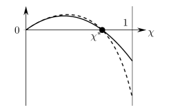
A The Krugman model

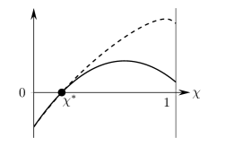
B The Helpman model

Figure 5: $G$ and $G^{\sharp}$ for the Krugman and Helpman models. For each model, the dashed curve illustrates $\omega=G(\chi)$, whereas the solid curve illustrates $\omega^{\sharp}\equiv G^{\sharp}(\chi)$.

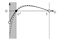
C The Krugman model

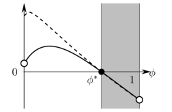
D The Helpman model

Figure 6: $\omega=G(\chi(\phi))$ (dashed curves) and $\omega^{\sharp}=G^{\sharp}(\chi(\phi))$ (solid curves).

We can check the stability of $\bar{\bm{x}}$ on the $\phi$ axis using Figure 6. The figure illustrates the composite functions $\omega=G(\chi(\phi))$ and $\omega^{\sharp}\equiv G^{\sharp}(\chi(\phi))$ for each model. As uniform distribution $\bar{\bm{x}}$ is stable if $\omega<0$ and unstable if $\omega>0$, and $G(\chi(\phi))=0$ gives the critical point of $\phi$ at which $\bar{\bm{x}}$ becomes unstable. For the Krugman model, $\bar{\bm{x}}$ is stable if $\phi<\phi^{*}\equiv\frac{1-\chi^{*}}{1+\chi^{*}}$ and unstable if $\phi>\phi^{*}$, where $\chi^{*}$ is the solution to $G(\chi)=0$ in Figure 6. Similarly, for the Helpman model, $\bar{\bm{x}}$ is stable if $\phi^{*}>\frac{1-\chi^{*}}{1+\chi^{*}}$ and unstable if $\phi<\phi^{*}$. The gray region in each figure in Figure 6 represents the range of $\phi$ where $\bar{\bm{x}}$ is stable. As expected, $\bar{\bm{x}}$ is stable for low (high) values of $\phi$ in the Krugman (Helpman) model and unstable otherwise.

3.2 Spatial scale of dispersion forces

The reverse scenario in the two-region economy stems from differences in the nature of their dispersion forces. In the Krugman model, the agglomeration (dispersion) force is captured by the first (second) term in (14). In the Helpman model, the second term in (15) reflects the agglomeration force, whereas the first and third terms the dispersion forces.

The agglomeration forces in the two models are equivalent; $C_{1}\chi$ in $\omega=G^{\sharp}(\chi)$ arises from the price index of the differentiated varieties (11). A region with a larger set of suppliers (firms) in the market has a lower price index. Mobile workers prefer such a region if the nominal wage is the same. The agglomeration force declines as $\phi$ increases as we confirm that $C_{1}\chi=C_{1}\frac{1-\phi}{1+\phi}$ is smaller when $\phi$ is larger.

The dispersion force in the Krugman model is the so-called market-crowding effect between firms (Baldwin-et-al-Book2003, Chapter 2). If a firm is geographically close to others, the firm can only pay a low nominal wage because of competition. Therefore, mobile workers are discouraged from entering a region where firms face fierce market competition with other firms in that location and nearby regions. The dispersion force thus depends on proximity structure $\mathbf{D}$ and appears as a negative second-order term, $-C_{2}\chi^{2}$. This force is stronger when $\chi$ is large (when $\phi$ is small).

The main dispersion force in the Helpman model, on the other hand, is local congestion effect from competition in the housing market of each region. The housing market does not depend on interregional proximity structure $\mathbf{D}$ but only on the mass of agents within each region. The force thus appears in $G^{\sharp}$ as negative constant term, $-(1-\mu)$. As the agglomeration force ($C_{1}\chi$) declines as $\phi$ increases, the relative strength of the dispersion force rises with $\phi$.

The key difference between the Krugman and Helpman models is whether the dispersion force acts between or within regions. To denote this distinction, we introduce the formal notion of spatial scale of dispersion forces.

We first introduce net gain functions that ignore the denominator of $G$, $G^{\flat}$, which is positive and thus irrelevant to the stability of $\bar{\bm{x}}$.

Definition 3.

A net gain function $G^{\sharp}$ for a canonical model with gain function $G$ is a lowest-order polynomial that satisfies $\operatorname{sgn}[G(\chi)]=\operatorname{sgn}[G^{\sharp}(\chi)]$ for all $\chi\in(0,1)$.

For example, the net gain functions for the Krugman and Helpman models are, respectively, given by (14) and (15), as $G^{\flat}(\chi)>0$ for all $\chi\in(0,1)$. For the Beckmann model, $G^{\sharp}(\chi)=G(\chi)=-\gamma+\chi$.

With this preparation, we can introduce the spatial scale of dispersion forces, which refines the definition of dispersion forces in Definition 2.

Definition 4 (Spatial scale of dispersion forces).

A negative constant term in the net gain function $G^{\sharp}$ is called a local dispersion force. The other negative terms in $G^{\sharp}$ are called global dispersion forces.

3.3 Three prototypical model classes

If either agglomeration force or dispersion force in a model is too strong, $\bar{\bm{x}}$ can be (un)stable for all levels of transport cost. To study endogenous agglomeration due to changes in the level of transport costs, we exclude parameter values for which no bifurcation occurs. In particular, we assume that $\bar{\bm{x}}$ is stable for some $\phi$ and unstable for some other $\phi$.

Assumption E (Endogenous agglomeration occurs).

The values of the model parameters are such that $G$ switches its sign at least once in $(0,1)$.

Under Assumption E, we introduce a formal classification of canonical models based on three prototypical shapes of $G$ found in the literature. The classification corresponds to the composition of the dispersion forces in the model (see Table 1 in Section 1).

Definition 5.

Suppose Assumption E. A canonical model with gain function $G$ is said to be:

1. Class I, if there is one and only one root $\chi^{*}\in(0,1)$ for $G$ such that $G(\chi)>0$ for $\chi\in(0,\chi^{*})$, $G(\chi^{*})=0$, and $G(\chi)<0$ for $\chi\in(\chi^{*},1)$.

2. Class II, if there is one and only one $\chi^{**}\in(0,1)$ such that $G(\chi)<0$ for $\chi\in(0,\chi^{**})$, $G(\chi^{**})=0$, and $G(\chi)>0$ for $\chi\in(\chi^{**},1)$.

3. Class III, if there are two and only two $\chi^{*},\chi^{**}\in(0,1)$ such that $G(\chi^{*})=G(\chi^{**})=0$ and $\chi^{**}<\chi^{*}$, with $G(\chi)<0$ for $\chi\in(0,\chi^{**})\cup(\chi^{*},1)$ and $G(\chi)>0$ for $\chi\in(\chi^{**},\chi^{*})$.

For example, the gain function of the Beckmann model (Example 2.1) is $G(\chi)=-\gamma+\chi$. If $\gamma\in(0,1)$, then $G$ has one and only one root $\chi^{*}=\gamma\in(0,1)$ and $G(\chi)<0$ for all $\chi<\chi^{*}$ and $G(\chi)>0$ for all $\chi>\chi^{*}$, satisfying Definition 5 (b). If $\gamma\geq 1$ ($\gamma\leq 0$), then $G$ has no root in $(0,1)$ and violates Assumption E, and $\bar{\bm{x}}$ is always stable (unstable). The gain functions of the Krugman and Helpman models have two parameters, $\mu\in(0,1)$ and $\sigma>1$ (Section 3.1). For the Krugman model, if $1<(1-\mu)\sigma$, $G$ behaves as Figure 5A illustrates, satisfying Definition 5 (a). If $1\geq(1-\mu)\sigma$, then $G(\chi)>0$ for all $\chi\in(0,1)$. This violates Assumption E and $\bar{\bm{x}}$ is always unstable (agglomeration force is too strong). For the Helpman model, if $1>(1-\mu)\sigma$, $G$ behaves as Figure 5B illustrates, satisfying Definition 5 (b). If $1\leq(1-\mu)\sigma$, $G(\chi)<0$ for all $\chi\in(0,1)$. This violates Assumption E and $\bar{\bm{x}}$ is always stable (dispersion force is strong). Other examples of the three model classes in the literature are provided below.

Example 3.3.

Class I includes Krugman-JPE1991, Puga-EER1999 (§3), Forslid-Ottaviano-JoEG2003, Pfluger-RSUE2003, and Harris-Wilson-EPA1978. ∎

Example 3.4.

Class II includes Helpman-Book1998, Murata-Thisse-JUE2005, Redding-Sturm-AER2008, Allen-Arkolakis-QJE2014, Redding-Rossi-Hansberg-ARE2017 (§3), and Beckmann-Book1976. ∎

Example 3.5.

Class III includes Tabuchi-JUE1998, Puga-EER1999 (§4), Pfluger-Suedekum-JUE2008, and Takayama-Akamatsu-JSCE2011. ∎

Definition 5 can be equivalently stated by net gain function $G^{\sharp}$. Although Definition 5 does not place any restriction on the functional form of $G$ or $G^{\sharp}$, net gain functions $G^{\sharp}$ for models in the literature, including those in the above examples, are usually simple quadratic functions with model-dependent coefficients $\{c_{0},c_{1},c_{2}\}$:

$$G^{\sharp}(\chi)=c_{0}+c_{1}\chi+c_{2}\chi^{2}.$$ (16)

The net gain functions for the Krugman and Helpman models are illustrated in (14) and (15) in Section 3.1. Appendix D provides the derivations of $\{c_{0},c_{1},c_{2}\}$ for the models by Krugman-JPE1991, Helpman-Book1998, Pfluger-Suedekum-JUE2008, and Allen-Arkolakis-QJE2014.

The coefficients $\{c_{0},c_{1},c_{2}\}$ in the quadratic representation (16) are some functions of the model parameters. A particular economic force in a model can impact several coefficients simultaneously because they are obtained by collecting the terms of $G^{\sharp}$ according to the order of $\chi$. By this rearrangement, we can focus on the “order” of endogenous economic forces in the model. In (16), $c_{0}$ summarizes all the forces that work within each location (whether negative or positive), which may be called the “zero-th order” spatial effects (or local forces). The latter two coefficients $\{c_{1},c_{2}\}$ correspond to global forces. The direct effects between regions (from one region to another) are summarized by $c_{1}$ and can be interpreted as the “first-order” spatial effects. Similarly, $c_{2}$ summarizes the “second-order” effects from region $k$ to region $j$, and then from region $j$ to region $i$. For example, in the Krugman and Helpman models, for a firm in region $i$, an increase in the number of competitors in region $k\neq i$ over demand in region $j$ ($\neq k\neq i$) may imply less demand from region $j$. The magnitude of such an effect will depend on both $\phi_{ij}$ and $\phi_{jk}$, and thus appears as a second-order term of $\mathbf{D}$.

For example, the Helpman model has the following net gain function:

$$G^{\sharp}(\chi) =\underbrace{-(1-\mu)}_{c_{0}}+\underbrace{\left(\dfrac{\mu}{\sigma-1}+\dfrac{\mu}{\sigma}\right)}_{c_{1}}\chi+\underbrace{\left(-\dfrac{\mu^{2}}{\sigma-1}-\dfrac{1}{\sigma}+(1-\mu)\right)}_{c_{2}}\chi^{2}.$$

Evidently, $\mu$ affects all the coefficients simultaneously, whereas $\sigma$ affects only $c_{1}$ and $c_{2}$. As $\mu$ is the expenditure share of manufactured goods, raising $\mu$ strengthens both agglomeration force $c_{1}\chi>0$ and global dispersion force $c_{2}\chi^{2}<0$ as $|c_{1}|$ and $|c_{2}|$ are increasing in $\mu$ under Assumption E, whereas it weakens the local dispersion force $c_{0}=-(1-\mu)<0$. To put it another way, an increase in expenditure share of housing $1-\mu$ strengthens the local dispersion force, but at the same time weakens the other forces related to differentiated goods as both $|c_{1}|$ and $|c_{2}|$ are decreasing in $1-\mu$. The coefficients $c_{1}$ and $c_{2}$ share the same terms with the Krugman model (14), as these models share common economic forces concerning differentiated goods. For detailed discussions on how economic forces in the Krugman and Helpman models are reflected in the coefficients in $G^{\sharp}$, see, respectively, Remark D.1 in Appendix D.2.1 and Remark D.4 in Appendix D.2.2.

Definition 5 (and Table 1) classifies canonical models based on the spatial scale of the “effective” dispersion forces. According to Definition 4, the Helpman model has global dispersion forces because $c_{2}<0$ under Assumption E. However, unlike the Krugman model, the global dispersion forces in the Helpman model ($c_{2}\chi^{2}<0$) are not “effective” in the sense that, under any admissible values of $\mu$ and $\sigma$, this force does not stabilize the uniform distribution for any level of transport costs. If we drop the local dispersion force $c_{0}<0$ from $G^{\sharp}$, we have $c_{1}\chi+c_{2}\chi^{2}>0$ for all $\chi$ and $\bar{\bm{x}}$ is always unstable. Thus, the only dispersion force in the Helpman model that can stabilize $\bar{\bm{x}}$ is its local dispersion force.

Definition 5 identifies three prototypical model classes found in the literature. Although extant models usually have restrictions on the values of their parameters that unambiguously determine the model class each belongs to, some flexible models can change their behavior depending on the parameter values. For example, the model by Pfluger-Tabuchi-RSUE2010 can fall into both Classes II and III depending on the parameter values. For such a model, one can split its parameter space to understand the model behavior in light of the three prototypical classes.

4 How model class matters

In the two-region economy, the differences in the spatial scales of dispersion forces in the Krugman and Helpman models induce the “reverse scenario” regarding the timing of endogenous asymmetry. In many-region economies, there is another contrast in whether endogenous spatial patterns become multimodal or unimodal. In this section, we consider canonical models in a many-region setting and establish Proposition 1 to provide a formal classification of these models in terms of endogenous spatial patterns.

4.1 Endogenous agglomeration in a racetrack economy

We start by explaining endogenous agglomeration under Assumptions RE and S. The uniform pattern $\bar{\bm{x}}\equiv(\bar{x},\bar{x},\ldots,\bar{x})$ ($\bar{x}\equiv\frac{1}{N}$) is always a spatial equilibrium. We are interested in the spatial patterns that emerge when $\bar{\bm{x}}$ becomes unstable.

Consider an infinitesimal migration of agents $\bm{z}=(z_{i})_{i\in\mathcal{N}}$ from $\bar{\bm{x}}$ so that the new spatial distribution becomes $\bm{x}^{\prime}\equiv\bar{\bm{x}}+\bm{z}$. Because the total mass of agents should not change, we require $\sum_{i\in\mathcal{N}}z_{i}=0$. Analogous to the two-region case, the marginal gain for agents due to such a deviation can be evaluated by the payoff elasticity matrix $\mathbf{V}=\frac{\bar{x}}{\bar{v}}\nabla\bm{v}(\bar{\bm{x}})$ as follows:

$$\bar{\omega}\equiv\bm{z}^{\top}\mathbf{V}\bm{z}.$$ (17)

If $\bar{\omega}<0$ for any $\bm{z}$, then $\bar{\bm{x}}$ is stable.

Under Assumptions RE and S, there is a model-independent way to conveniently represent all possible migration patterns $\bm{z}$. Specifically, we can write

$$\bm{z}=\sum_{k}\zeta_{k}\bm{z}_{k},$$ (18)

where $\{\bm{z}_{k}\}$ are the eigenvectors of $\mathbf{V}$ satisfying $\bm{z}_{k}^{\top}\bm{z}_{l}=0$ for $k\neq l$, and $\{\zeta_{k}\}$ are their coefficients. We normalize $\|\bm{z}_{k}\|^{2}=\bm{z}_{k}^{\top}\bm{z}_{k}=1$ for all $k$. By (18), we interpret $\bm{z}$ as the weighted sum of the “basic” migration patterns $\{\bm{z}_{k}\}$. The basic migration patterns are model-independent in the sense that they are the eigenvectors of $\mathbf{V}$ irrespective of the properties of the payoff function $\bm{v}$ other than Assumption S.

In the two-region economy, $\bm{z}=(1,-1)$ is the only possible migration pattern. The many-region economy allows multiple possibilities. Each $\bm{z}_{k}$ represents a $k$-modal migration pattern and is expressed by a cosine curve with $k$ equally spaced peaks. The largest number of peaks is $k=\frac{N}{2}$ because the concentration of agents in every other region achieves the maximum number of symmetric peaks.

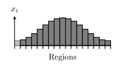
A Unimodal agglomeration ($\bar{\bm{x}}+\zeta\bm{z}_{1}$)

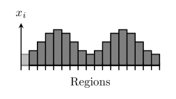
B Bimodal agglomeration ($\bar{\bm{x}}+\zeta\bm{z}_{2}$)

C Quad-modal agglomeration ($\bar{\bm{x}}+\zeta\bm{z}_{4}$)

D Octa-modal agglomeration ($\bar{\bm{x}}+\zeta\bm{z}_{8}$)

Figure 7: Schematic illustrations of spatial patterns induced by each migration pattern ($N=16$). The cases when $k$ is a power of $2$ are presented.

Figure 7 shows spatial patterns $\bar{\bm{x}}+\zeta\bm{z}_{k}$ ($k=1$, $2$, $4$, $8$) for $N=16$ with small $\zeta>0$. Basic migration patterns $\bm{z}_{1}$, $\bm{z}_{2}$, $\bm{z}_{4}$, and $\bm{z}_{8}$ express, respectively, the formation of a uni-, bi-, quad- and octa-modal agglomerations, respectively.

Let $\omega_{k}$ be the eigenvalue of $\mathbf{V}$ associated with $\bm{z}_{k}$. Then,

$$\bar{\omega}=\bm{z}^{\top}\mathbf{V}\bm{z}=\big{(}\sum_{k}\zeta_{k}\bm{z}_{k}\big{)}^{\top}\mathbf{V}\big{(}\sum_{k}\zeta_{k}\bm{z}_{k}\big{)}=\sum_{k}\zeta_{k}^{2}\bm{z}_{k}^{\top}\mathbf{V}\bm{z}_{k}=\sum_{k}\zeta_{k}^{2}\omega_{k}$$ (19)

because $\bm{z}_{k}^{\top}\bm{z}_{l}=0$ for $k\neq l$ and $\omega_{k}\bm{z}_{k}=\mathbf{V}\bm{z}_{k}$. Thus, $\bar{\omega}$ is maximized by choosing the basic migration pattern that has the largest eigenvalue:

$$\max_{\bm{z}}\ \bar{\omega}=\omega_{\text{max}}\text{\quad where \quad}\omega_{\text{max}}\equiv\max_{k}\ \{\omega_{k}\}.$$ (20)

If $\omega_{\text{max}}<0$, then $\bar{\bm{x}}$ is stable; when $\omega_{\text{max}}$ turns to positive, $\bar{\bm{x}}$ becomes unstable. Each $\omega_{k}$ is the gain from migration towards $\bm{z}_{k}$’s direction, and $\bar{\bm{x}}$ becomes unstable when some migration direction becomes profitable. The spatial pattern that emerges at the onset of instability is $\bar{\bm{x}}+\zeta\bm{z}_{\text{max}}$, where $\bm{z}_{\text{max}}$ is the basic migration pattern associated with $\omega_{\text{max}}$. This generalizes the discussion based on $\omega$ and $\bm{z}=(1,-1)$ in the two-region case.

We need the specific formulae for eigenvalues $\{\omega_{k}\}$ of $\mathbf{V}$. For canonical models, we have $\mathbf{V}=G(\bar{\mathbf{D}})$ where $\bar{\mathbf{D}}$ is the row-normalized proximity matrix, and $G$ is a rational function. Under this condition, the two-region formula $\omega=G(\chi)$ generalizes as follows:

$$\omega_{k}=G(\chi_{k}) \forall k,$$ (21)

where $\chi_{k}$ is the eigenvalue of $\bar{\mathbf{D}}$ associated with $\bm{z}_{k}$.

Each $\chi_{k}$ is an index of the marginal increase of the average proximity among agents when the $k$-modal pattern $\bar{\bm{x}}+\zeta\bm{z}_{k}$ emerges. Further, $\chi_{k}$ decreases in the number of peaks $k$ under Assumption RE. This is because the average proximity from one agent to other agents is the largest in a unimodal pattern as in Figure 7A. As the number of peaks in the spatial distribution increases, the average proximity between agents decreases. In fact, under Assumption RE,

$$\max_{k}\{\chi_{k}\}=\chi_{1}\quad\text{and}\quad\min_{k}\{\chi_{k}\}=\chi_{\frac{N}{2}}$$ (22)

for any given value of $\phi\in(0,1)$ (Akamatsu-Takayama-Ikeda-JEDC2012), where we recall that the maximum possible number of symmetric peaks is $\frac{N}{2}$. Every $\chi_{k}$ takes values on $(0,1)$ and is a decreasing function of $\phi$, reflecting that, irrespective of $k$, the proximity of an agent to others increases monotonically when the freeness of interregional interactions increases monotonically.

4.2 Endogenous spatial patterns for the three model classes

In the general derivation above, the properties of the symmetric racetrack geography are summarized by $\{\bm{z}_{k}\}$ and $\{\chi_{k}\}$, while gain function $G$ encapsulates the other model-dependent properties of the payoff function $\bm{v}$. That said, $\omega_{\text{\text{max}}}=\max_{k}\omega_{k}=\max_{k}G(\chi_{k})$ at the onset of instability depends on the properties of $G$. Thus, the model class matters.

The simplest example is the Beckmann model, which is Class II. As $G(\chi)=-\gamma+\chi$ and $\max_{k}\{\chi_{k}\}=\chi_{1}$, we see

$$\omega_{\text{max}}=\max_{k}\{\omega_{k}\}=\max_{k}\{G(\chi_{k})\}=\max_{k}\{-\gamma+\chi_{k}\}=-\gamma+\max_{k}\{\chi_{k}\}=-\gamma+\chi_{1}.$$

This means that, for mobile agents in the model, $\bm{z}_{1}$ is the most profitable migration pattern at any given $\phi$, and instability of $\bar{\bm{x}}$ leads to the formation of a unimodal agglomeration (Figure 7A). The maximality of $\omega_{1}$ is intuitive. In the model, a unimodal distribution is the most beneficial outcome as agents prefer proximity to others, albeit agents must locally disperse to avoid congestion. This argument can be simply understood by drawing the curves of $\{\omega_{k}\}$ on the $\phi$ axis. Figure 8A shows $\{\omega_{k}\}$ for the Beckmann model with $N=16$. When all the curves stay below $\phi$ axis, $\bar{\bm{x}}$ is stable (the gray region). When one and only one $\omega_{k}$ cuts the axis, then $\bar{\bm{x}}$ deviates in $\bm{z}_{k}$ direction. Obviously, $\omega_{1}$ is the first to cut the axis from below.

With the same line of logic as this example, we can show the following proposition to characterize the endogenous spatial patterns that emerge in Class I, II, or III models when $\bar{\bm{x}}$ becomes unstable (see Appendix B for proof).

Proposition 1.

Suppose Assumptions RE, S, and E. Consider a canonical model.

1. If the model is of Class I, then there exists $\phi^{*}\in(0,1)$ such that $\bar{\bm{x}}$ is stable for all $\phi\in(0,\phi^{*})$ and unstable for all $\phi\in(\phi^{*},1)$. The instability of $\bar{\bm{x}}$ at $\phi^{*}$ leads to the formation of a multimodal pattern with $\frac{N}{2}$ peaks.

2. If the model is of Class II, there exists $\phi^{**}\in(0,1)$ so that $\bar{\bm{x}}$ is stable for all $\phi\in(\phi^{**},1)$ and unstable for all $\phi\in(0,\phi^{**})$. The instability of $\bar{\bm{x}}$ at $\phi^{**}$ leads to the formation of a unimodal pattern.

3. If the model is of Class III, there exist $\phi^{*},\phi^{**}\in(0,1)$ with $\phi^{*}<\phi^{**}$ so that $\bar{\bm{x}}$ is stable for all $\phi\in(0,\phi^{*})\cup(\phi^{**},1)$. The instabilities of $\bar{\bm{x}}$ at $\phi^{*}$ and $\phi^{**}$ lead to the formation of a multimodal pattern with $\frac{N}{2}$ peaks and a unimodal pattern, respectively.

Note that (a) and (b) generalizes the “reversed scenarios” of the two-region Krugman and Helpman models in that $\bar{\bm{x}}$ is stable for the low (high) values of $\phi$ in Class I (II) models. The new phenomenon is that model classes qualitatively differ in the number of peaks they endogenously produce. Class I models produce a $\frac{N}{2}$-modal distribution, which can be interpreted as the formation of $\frac{N}{2}$ small cities. Class II models entail a unimodal distribution, which can be interpreted as the formation of a large economic agglomeration extending over multiple regions. Class III is a synthesis of Classes I and II. If $N=16$, the instability at $\phi^{*}$ in Classes I and III leads to the formation of octa-modal pattern (Figure 7D), whereas that at $\phi^{**}$ in Classes II and III leads to the formation of unimodal pattern (Figure 7A). These contrasts in spatial patterns are hidden in the two-region setup as $\bm{z}=(1,-1)$ is the only possible migration pattern.

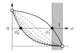
A The Beckmann model (Class II)

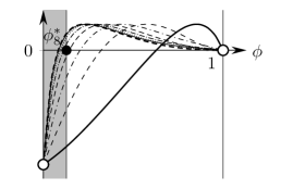
B The Krugman model (Class I)

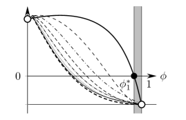
C The Helpman model (Class II)

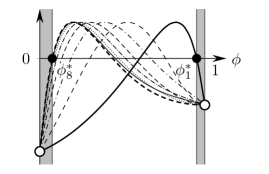
D The Pflüger–Südekum model (Class III)

Figure 8: Examples of $\omega_{k}=G(\chi_{k}(\phi))$ when $N=16$. $\phi_{k}^{*}$ indicates a solution to $\omega_{k}(\phi)=0$. See also Figure B.1. It is noted that Panel (A) illustrates the shapes of $\{\chi_{k}\}$ on the $\phi$ axis.

The curves of $\{\omega_{k}\}$ for representative examples of general equilibrium models from the three classes are shown in Figure 8 for the $N=16$ case. Figure 8B and Figure 8C respectively depict $\{\omega_{k}\}$ for the Krugman and Helpman models as the leading examples of Classes I and II. In the ranges of $\phi$ where $\bar{\bm{x}}$ is stable (the gray regions), $\max\{\omega_{k}\}=\omega_{8}$ for the Krugman model, whereas $\max\{\omega_{k}\}=\omega_{1}$ for the Helpman model, which are consequences of the maximality of $\chi_{1}$ and the minimality of $\chi_{\frac{N}{2}}$ (see Figure B.1). Thus, when $\bar{\bm{x}}$ becomes unstable, $\frac{16}{2}=8$-modal agglomeration as in Figure 7D emerges for the former model, whereas a unimodal agglomeration as in Figure 7A emerges for the latter. Figure 8D shows $\{\omega_{k}\}$ for an instance of Class III, the Pfluger-Suedekum-JUE2008 model. There are two ranges of $\phi$ under which $\bar{\bm{x}}$ is stable. With both local and global dispersion forces, the model behaves as a Class I (II) model at lower (higher) values of $\phi$. Octa-modal agglomeration emerges at $\phi_{8}^{*}$ as in the Krugman model and a unimodal agglomeration emerges at $\phi_{1}^{*}$ as in the Helpman model.

4.3 Evolution of spatial patterns

Proposition 1 builds on local analysis around uniform distribution $\bar{\bm{x}}$ and characterizes bifurcations from $\bar{\bm{x}}$. It does not consider “global” behavior, that is, the whole evolutionary path of spatial equilibria along the $\phi$ axis. To proceed beyond the local result, we must assume a specific payoff function instead of the general class of canonical models (Definition 1). Indeed, it is often possible to formally study global behavior in detail beyond Proposition 1 by considering a specific model (payoff function $\bm{v}$). For specific Class I models, it can be demonstrated that successive “period-doubling” bifurcations can occur. The number of agglomerations typically evolves as $N\to\frac{N}{2}\to\frac{N}{4}\to\ldots$ so long as it remains to be an integer (Akamatsu-Takayama-Ikeda-JEDC2012; ikeda2012spatial; Osawa-et-al-JRS2017). For Class II models, Takayama-Ikeda-Thisse-RSUE2020 provides a detailed analysis of Murata-Thisse-JUE2005 model in a racetrack economy to demonstrate single-peaked spatial distributions emerge. Also, AMT-2016 formally shows that, in the four-region racetrack economy, Helpman-Book1998 model produces unimodal configuration, and multimodal agglomeration cannot become stable when the symmetric dispersion is unstable.

A caveat is that the formal analyses of the models’ global behavior suffer from severe model dependence without changing qualitative implications regarding whether spatial configurations become unimodal or multimodal. Instead of model-specific theory, we provide numerical examples to illustrate representative agglomeration behavior for each model class. Figure 9 illustrates the typical global behaviors of the three model classes on the $N=16$ racetrack economy. We follow a path of stable spatial distribution branching from $\bar{\bm{x}}$, from $\phi=0$ (high transport costs) to $\phi=1$ (low transport costs). The lower in each figure, the higher the freeness of transport $\phi$. For interpretability, the spatial distributions in the racetrack economy are visualized on a line segment, so that the leftmost region is neighboring to the rightmost region.

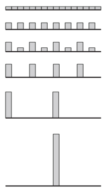
A Class I

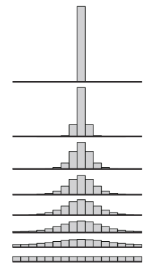
B Class II

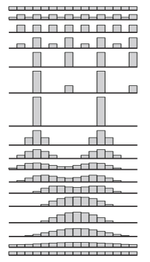
C Class III

Figure 9: Stable spatial patterns at different transport cost levels.

Figure 9A considers a Class I model, the Krugman model. The stable spatial configuration starts from a uniform distribution when $\phi$ is small. A multimodal distribution with $\frac{16}{2}=8$ agglomerations endogenously emerges when $\phi$ reaches the critical value [Proposition 1 (a)]. Through successive symmetry-breaking bifurcations, an increase in $\phi$ induces a decrease in the number of agglomerations, an increase in the spacing between them, and an increase in the size of each agglomeration. The number of agglomerations evolves as $16\to 8\to 4\to 2\to 1$.

By contrast, in Class II models, only unimodal distributions emerge endogenously. Figure 9B considers the Helpman model. The uniform distribution $\bar{\bm{x}}$ is unstable when $\phi$ is small and agents concentrate around a single peak. When the transport cost decreases, it causes the flattening of the single agglomeration as the peak population density is reduced. At the critical level of $\phi$, the spatial distribution becomes uniform [Proposition 1 (b)].

Class III is a synthesis of Classes I and II. Figure 9C considers a Class III model proposed by Pfluger-Suedekum-JUE2008. The uniform distribution is stable when $\phi$ is small. As $\phi$ increases, octa-modal agglomerations emerge at some point as in Class I models. At moderate levels of transport cost, multiple bell-shaped agglomerations are generated. For this range, a decrease in transport costs causes a decrease in the number of agglomerations (as in Class I models) and the flattening of each agglomeration (as in Class II models). When $\phi$ is close to one, the spatial distribution becomes unimodal, similar to the Class II model in Figure 9B. The overall behavior of the Class III model is qualitatively consistent with the evolution of Japanese urban agglomerations discussed in Section 1.

As further examples, Appendix C provides numerical simulations for the $N=8$ case with bifurcation diagrams and discussions on various connections to the empirical literature. Also, Appendix E provides numerical simulations for the case we drop Assumption RE by considering a long narrow economy and a square economy. Qualitative contrasts between model classes regarding the number, size, and spatial extent of cities generalize beyond the symmetric racetrack economy.

5 Regional heterogeneities

To focus on endogenous mechanisms, Proposition 1 abstracts away exogenous geographical asymmetry among regions due to their relative position in the transport network and other idiosyncratic regional characteristics (RE and S). It is of interest to what extent the implications of Proposition 1 generalize to asymmetric cases, given that quantitative spatial models in the literature incorporate flexible structures regarding interregional transport costs and differences in regional characteristics (Redding-Rossi-Hansberg-ARE2017).

Throughout this section, we retain Assumption RE and focus on the marginal roles of local regional characteristics by relaxing Assumption S. Specifically, we study the sensitivity of spatial patterns to regional characteristics such as local amenities and productivity differences. We show that a model’s spatial scale of dispersion force(s) tends to govern whether the effects of exogenous advantages are amplified when transport cost varies.

Let $\bm{a}=(a_{i})_{i\in\mathcal{N}}$ with $a_{i}>0$ be exogenous characteristics of region $i$, which may or may not affect the payoffs in other regions, so that the payoff function becomes $\bm{v}(\bm{x},\bm{a})$. For example, $a_{i}$ may be the level of exogenous amenities in region $i$ or region $i$’s exogenous productivity. In the latter case, trade flows and the resulting payoffs in other regions can depend on $a_{i}$.

The regions are symmetric if $\bm{a}=\bar{\bm{a}}\equiv(\bar{a},\bar{a},\ldots,\bar{a})$, for some $\bar{a}>0$. Therefore, $(\bar{\bm{x}},\bar{\bm{a}})$ is an equilibrium. To introduce regional heterogeneity, consider an infinitesimal variation in the local characteristic so that $\bm{a}=\bar{\bm{a}}+\bm{\epsilon}$ with small $\bm{\epsilon}=(\epsilon_{i})_{i\in\mathcal{N}}$. Suppose there is a new equilibrium, say $\bm{x}(\bm{a})$, which is close to $\bar{\bm{x}}$. The “covariance” between region $i$’s relative (dis)advantage $\epsilon_{i}=a_{i}-\bar{a}$ and the relative deviation of its population from the uniformity, $x_{i}(\bm{a})-\bar{x}$, is given by:

$$\rho\equiv(\bm{a}-\bar{\bm{a}})^{\top}\left(\bm{x}(\bm{a})-\bar{\bm{x}}\right)=\sum_{i\in\mathcal{N}}\left(a_{i}-\bar{a}\right)\left(x_{i}(\bm{a})-\bar{x}\right).$$ (23)

We assume that $\bar{\bm{x}}$ is stable as otherwise considering $\bm{x}(\bm{a})$ is nonsensical. This is also in line with the quantitative literature where the uniqueness of equilibrium is often assumed (e.g. Redding-Sturm-AER2008; Allen-Arkolakis-QJE2014).

We focus on a class of local characteristics that acts positively in the payoff for agents. For this, we suppose $\bm{a}$ satisfies $\rho>0$. Let $\mathbf{A}\equiv\frac{\bar{a}}{\bar{v}}[\frac{\partial v_{i}}{\partial a_{j}}]$ be the elasticity matrix of the payoff regarding $\bm{a}$, evaluated at $(\bar{\bm{x}},\bar{\bm{a}})$. We suppose the following.

Assumption A.

For the local characteristic $\bm{a}$ under consideration, there is a rational function $G^{\natural}$ that is continuous over $[0,1]$, positive whenever $\bar{\bm{x}}$ is stable, and satisfies $\mathbf{A}=G^{\natural}(\bar{\mathbf{D}})$.

For each model in Examples 3.3–3.5, there is $G^{\natural}$ that satisfies the hypotheses of Assumption A for each choice of a local characteristic vector. The simplest example is local amenity.

Example 5.1.

Assume that the payoff function is $v_{i}(\bm{x},\bm{a})=a_{i}v_{i}(\bm{x})$, where $a_{i}>0$ is the exogenous level of regional amenities and $\bm{v}(\bm{x})=(v_{i}(\bm{x}))_{i\in\mathcal{N}}$ is the homogeneous component of the payoff function satysifying Assumption S. Then, $\mathbf{A}=\frac{\bar{a}}{\bar{v}}\bar{v}\mathbf{I}=\bar{a}\mathbf{I}$ and $G^{\natural}(\cdot)=\bar{a}>0$. ∎

Analogous to gain function $G$ of a model, $G^{\natural}$ summarizes the effect of the marginal changes in local characteristics $\bm{a}$ on the regional payoffs $\bm{v}$. Particularly, $G^{\natural}(\cdot)>0$ implies $\rho>0$.

Example 5.2.

In a symmetric two-region economy, whenever $\bar{\bm{x}}$ is stable,

$$\rho=c\delta(\chi)\quad\text{where}\quad\delta(\chi)\equiv-\dfrac{G^{\natural}(\chi)}{G(\chi)}\quad\text{and}\quad\chi=\frac{1-\phi}{1+\phi}$$ (24)

with some $c>0$. If $\bar{\bm{x}}$ is stable, $\omega=G(\chi)<0$. Thus, $\rho>0$ if $G^{\natural}(\chi)>0$ for all $\chi$ with $\omega=G(\chi)<0$. To show (24), note that the marginal payoff gain due to exogenous advantage in region $1$ can be summarized by the following elasticity:

$$\alpha\equiv\frac{\bar{a}}{\bar{v}}\left(\dfrac{\partial{v_{1}(\bar{\bm{x}},\bar{\bm{a}})}}{\partial{a_{1}}}-\dfrac{\partial{v_{2}(\bar{\bm{x}},\bar{\bm{a}})}}{\partial{a_{1}}}\right)$$ (25)

where $\alpha$ is the eigenvalue of $\mathbf{A}$ associated with $\bm{z}=(1,-1)$. Under Assumption A, $\alpha=G^{\natural}(\chi)>0$. Suppose $\bar{\bm{x}}=(\bar{x},\bar{x})$ is perturbed to $\bm{x}=(\bar{x}+\xi,\bar{x}-\xi)$ due to an exogenous regional asymmetry of the form $\bm{a}=(\bar{a}+\epsilon,\bar{a}-\epsilon)$ with small $\xi$ and $\epsilon$. As $\bm{x}$ is an equilibrium, $v_{1}(\bm{x})=v_{2}(\bm{x})$. Thus, $\xi$ and $\epsilon$ should cancel out two forces, namely, gain (or loss, as $\bar{\bm{x}}$ is stable) $\omega=G(\chi)<0$ from endogenous migration and gain $\alpha>0$ from exogenous asymmetry. We have $\omega\xi+\alpha\epsilon=0$, so that $\xi=-\frac{\alpha}{\omega}\epsilon=-\frac{G^{\natural}(\chi)}{G(\chi)}\epsilon$ and we obtain (24) with $c=2\epsilon^{2}$ as $\rho=\epsilon\xi+(-\epsilon)(-\xi)=2\epsilon\xi$. The fraction $\delta(\chi)=\frac{G^{\natural}(\chi)}{|G(\chi)|}=\frac{\alpha}{|\omega|}$ compares the magnitudes of gain from marginal exogenous advantage and of loss from marginal endogenous migration around $\bar{\bm{x}}$. ∎

An important question is whether $\rho$ increases or decreases when $\phi$ increases. In other words, does improved transportation access strengthen (weaken) the role of local characteristics and what are the responses of the spatial distribution of economic activities to an improvement in interregional access if $\bm{a}$ is fixed? The response of $\rho$ is a prototypical version of the questions asked in counterfactual exercises employing calibrated quantitative spatial economic models (see, e.g., Redding-Rossi-Hansberg-ARE2017, for a survey).

We characterize the response of $\rho$ to changes in $\phi$ as follows.

Proposition 2.

Suppose Assumption RE. Consider a canonical model with gain function $G$. Take local characteristic $\bm{a}$ that satisfies Assumption A with some $G^{\natural}$. Assume that $\bar{\bm{x}}$ is stable and define $\delta(\cdot)=-\frac{G^{\natural}(\cdot)}{G(\cdot)}$. Then, the following hold true for $\rho$ in (23):

1. $\rho^{\prime}(\phi)>0$, if $\delta^{\prime}(\chi)<0$ for all $\chi\in(0,1)$ such that $G(\chi)<0$.

2. $\rho^{\prime}(\phi)<0$, if $\delta^{\prime}(\chi)>0$ for all $\chi\in(0,1)$ such that $G(\chi)<0$.

The impacts of improved interregional access are obviously model dependent. However, model class matters. For simple cases, the response of $\rho$ under a given model can be inferred by the spatial scale of the dispersion force in the model.

When we consider heterogeneous local amenity (Example 5.1), there is a clear contrast between the Krugman (Class I) and Helpman (Class II) models.

Example 5.3.

Suppose $G^{\natural}(\cdot)=\bar{a}>0$ as in Example 5.1. Then, $\operatorname{sgn}[\delta^{\prime}(\cdot)]=\operatorname{sgn}[\frac{\bar{a}G^{\prime}(\cdot)}{G(\cdot)^{2}}]=\operatorname{sgn}[G^{\prime}(\cdot)]$. The Krugman model (Example 3.1) satisfies $G^{\prime}(\chi)<0$ whenever $G(\chi)<0$ (Figure 5A) and thus $\rho^{\prime}(\phi)>0$. The Helpman model (Example 3.2) satisfies $G^{\prime}(\chi)>0$ whenever $G(\chi)<0$ (Figure 5B) and thus $\rho^{\prime}(\phi)<0$ whenever the equilibrium is unique as assumed in quantitative applications. ∎

To see why such contrast emerges, considering a two-region setup suffices.

Example 5.4 (Example 5.2, continued).

For $N=2$, we have $\rho(\phi)=c\delta(\chi(\phi))$ with $\chi=\frac{1-\phi}{1+\phi}$. We have $\rho^{\prime}(\phi)=c\delta^{\prime}(\chi(\phi))\chi^{\prime}(\phi)$ where $\chi^{\prime}(\phi)<0$. For example, suppose that $\delta^{\prime}(\chi)<0$. We observe that, in general, $\delta^{\prime}(\chi)<0$ means either gain $\alpha=G^{\natural}(\chi)$ from the exogenous regional asymmetry decreases in $\chi$ or the magnitude of loss $|\omega|=|G(\chi)|$ from the endogenous migration increases in $\chi$. This is satisfied in Class I models. In Class I models, $|\omega|$ decreases in $\phi$ (i.e., increases in $\chi$) as long as $\bar{\bm{x}}$ is stable, because $\omega$ approaches to zero at the bifurcation point. When $G^{\natural}$ is constant, then we expect $\delta^{\prime}(\cdot)<0$ in Class I models because $\delta$ is inversely proportional to $|\omega|$. A similar discussion applies to Class II models, and we can expect that Class II models satisfy $\delta^{\prime}(\cdot)>0$. ∎

The contrast between Classes I and II generalizes to the regional characteristics that indirectly affect payoffs in the other regions.

Example 5.5.

The Krugman model (Example 3.1) is of Class I. In the model, $\bm{l}=(l_{i})_{i\in\mathcal{N}}$ can be regarded as a regional characteristic vector. For this model, $G^{\natural}$ is nonconstant but positive for all $[0,1]$. Also, $\delta^{\prime}(\chi)<0$ for all $\chi\in(0,1)$, so that $\rho^{\prime}(\phi)>0$, if $\bar{\bm{x}}$ is stable. See Remark D.3 in Appendix D. ∎

Example 5.6.

Redding-Rossi-Hansberg-ARE2017 studies a Class II model, namely the Helpman model with a modified market equilibrium condition:

$$w_{i}x_{i}=\sum_{j\in\mathcal{N}}\dfrac{x_{i}a_{i}w_{i}^{1-\sigma}\phi_{ij}}{\sum_{k\in\mathcal{N}}x_{k}a_{k}w_{k}^{1-\sigma}\phi_{kj}}w_{j}x_{j} \forall i\in\mathcal{N},$$ (26)

where $\bm{a}$ represents productivity differences. We have $G^{\natural}(\cdot)>0$ for all $[0,1]$. When equilibrium is unique, $\delta^{\prime}(\chi)>0$ for all $\chi\in(0,1)$ and thus $\rho^{\prime}(\phi)<0$. See Remark D.6 in Appendix D. ∎

Examples 5.3, 5.6, and 5.5 demonstrate that the spatial scale of dispersion forces in a model can determine whether the endogenous causation of the model strengthens the exogenous advantages when interregional transport costs change. When interregional access improves, the endogenous mechanisms of a model strengthen (weakens) the effects of exogenous local advantages if the model has only a global (local) dispersion force. If exogenous heterogeneity causes one region to attract more population, such effects will be magnified in Class I models, while they are reduced in Class II models.

The qualitative differences between Classes I and II can be understood from the basic properties of the local and global dispersion forces in Section 3.2. For a Class I model, a larger $\phi$ means a relatively weaker global dispersion force, which tends to amplify (both endogenous and exogenous) location-specific advantages towards the concentration of mobile agents. However, in a Class II model, a larger $\phi$ means a relatively stronger local dispersion force, which reduces not only the benefits from concentration due to endogenous agglomeration externalities but also those due to location-specific exogenous advantages.

Proposition 2 builds on local sensitivity analysis at $\bar{\bm{x}}$. Appendix F provides numerical examples for the eight-region case to confirm the implications of Proposition 2 are valid under nonmarginal asymmetry. It is an important empirical question to what extent these results generalize quantitatively when large regional heterogeneities as in reality are present.

6 Concluding remarks

This study has demonstrated that in many-region models of endogenous agglomeration, the spatial scale (local or global) of the dispersion force in a model governs the endogenous spatial patterns and comparative statics of the model. Three prototypical model classes were identified according to the spatial scale of their dispersion forces (i.e., only local, only global, and both local and global; Table 1).

Several aspects deserve further research. First, generalizing the theoretical results to different proximity structures is important. An efficient strategy would be to fix a few representative models (instead of geography) as test pilots and identify general insights when the proximity structure systematically varies (Matsuyama-RIE2017). The important implications of Proposition 1 on endogenous spatial patterns (whether a model produces unimodal or multimodal patterns) may be robust to generalizations of assumed geography, as discussed in Appendix E.

Second, it is important to consider multiple types of mobile agents subject to different proximity matrices and/or degrees of increasing returns. Such a structure is ubiquitous in multiple-sector models (Fujita-et-al-EER1999; Hsu-EJ2012; Gaubert-AER2018; Davis-Dingel-JIE2020) and intra-city models with both firms and households (e.g., Fujita-Ogawa-RSUE1982; Lucas-Rossi-Hansberg-ECTA2002; Ahlfeldt-et-al-ECTA2015; Heblich-etal-QJE2020). The racetrack economy provides a good starting point for analyzing these models (Tabuchi-Thisse-JUE2011; Osawa-Akamatsu-DP2019). Multiple-sector models are also important for understanding the mechanisms behind the remarkable regularities in size and spatial variations of economic agglomerations in the real world. For example, Mori-etal-PNAS2020 use the data from six countries, including the US, to demonstrate that the spatial common power law holds, that is, city-size distributions exhibit similar power laws both in the country and its spatial sub-regions. Notably, a multi-sector economic geography model can replicate common power laws in a symmetric racetrack economy (Mori-et-al-DP2022).

Finally, models featuring a continuum of agents, as in this study, are complementary to the recent development of granular spatial models (e.g., Ahlfeldt-et-al-CEPR2022) in which endogenous agglomeration arises from the increasing returns and indivisibility of agents. While continuum models (e.g., Hsu-EJ2012; Tabuchi-Thisse-JUE2011; Mori-et-al-DP2022) can endogenously replicate the systematic regularities such as the periodic agglomeration patterns, and city-size power laws including their fractal structure (Mori-etal-PNAS2020), granular spatial models are better at explaining idiosyncratic location choice behavior by superstar firms and plants (e.g., Greenstone-et-al-JPE2010). Combining these two approaches may provide a fundamental explanation for the spatial economy through endogenous mechanisms.

Appendix A Cities and transport network in Japan

We construct cities from the Grid Square Statistics of the Population Census in 1970–2020 (every five years). We define a city as an urban agglomeration (UA) as a set of contiguous 1 km-by-1 km cells whose population density is at least 1000/km² and a total population of at least 10,000. The results are robust for alternative threshold densities and populations. Fig. A.1 illustrates the identified 431 UAs in 2020. They occupy 80% of the national population and 8% of inhabitable land. The grey area indicates populated cells but a population density of less than 1,000, whereas darker cells have a larger population. As indicated in the figure, we consider only the cells reachable from four major islands, Hokkaido, Honshu, Shikoku, and Kyushu.

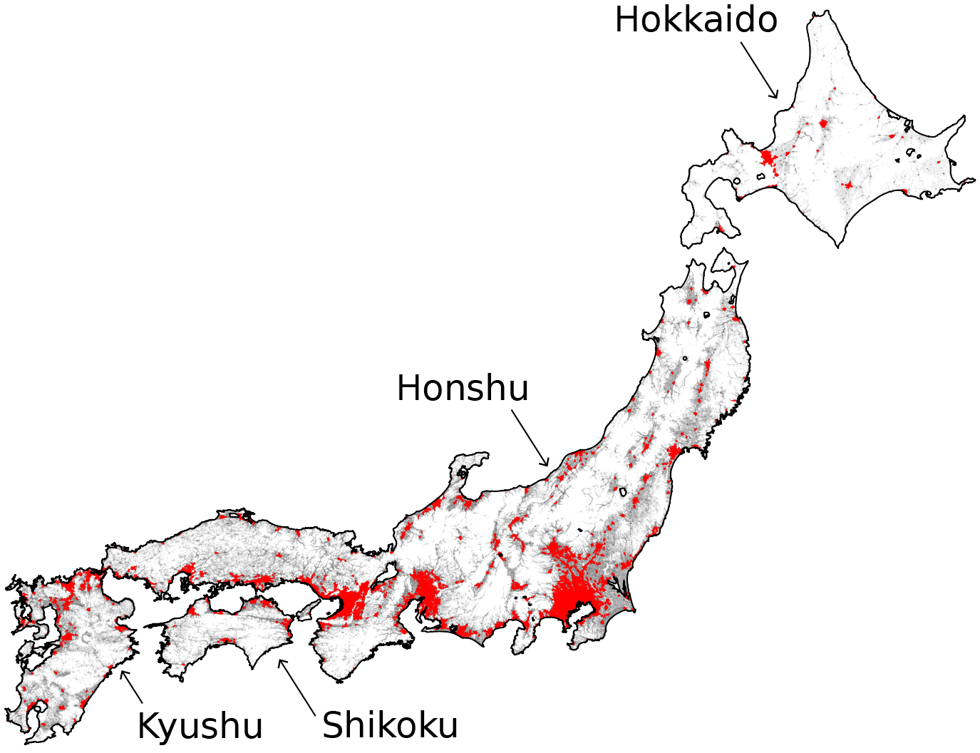
Figure A.1: Urban agglomerations of Japan in 2020

UAs are identified for each census year during the 1970–2020 period. Unique IDs throughout the period are assigned by the following steps.

1. IDs for the UAs in $t=1970$ are set to be their city-size ranking in the year.

2. A UA in year $t$ and a UA in year $t+5$ are considered the same if they mutually have the largest population in their areal intersection. In that case, their IDs in year $t+5$ are inherited from year $t$.

3. If UA $i$ in year $t$ has the largest population (in year $t$) in the areal intersection with UA $j$ in year $t+5$, and UA $j$ in year $t+5$ has the largest population in the areal intersection with a UA other than $i$ in year $t$, then UA $i$ is absorbed to UA $j$ in year $t+5$.

4. If UA $j$ in year $t+5$ has no intersection with any UA in year $t$, then UA $j$ is either a newly formed UA or a UA split from the existing UA. For a newly formed UA or a split UA with no predecessor in older years $<t$, a new ID is assigned in the order of their population size in year $t+5$.

5. If a UA is split from the existing UA in year $t+5$ but has a predecessor a year before $t$, the latest predecessor’s ID is recovered. If there are multiple latest predecessors, the one with the largest population in the areal intersection with the UA is chosen. Thus, a UA $i$, which was absorbed to another UA $j$ and then split from UA $j$, will be named $i$ again.

Fig. A.2A and B depict the development of high-speed railway and highway networks, respectively, in Japan between 1970 and 2020.

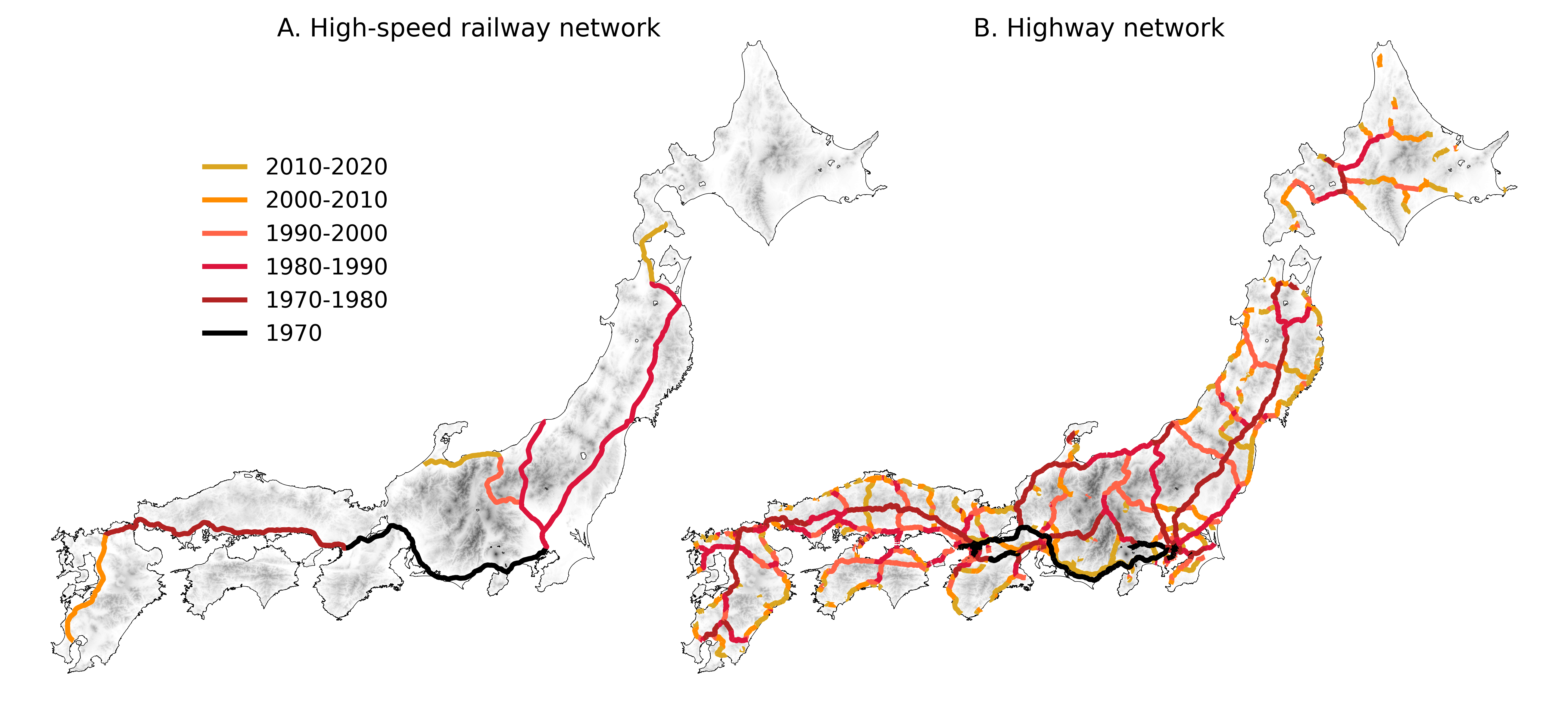
Figure A.2: The development of high-speed network in Japan

Appendix B Proofs

B.1 Proof of Proposition 1

We characterize the stability of $\bar{\bm{x}}=(\bar{x},\ldots,\bar{x})$ and bifurcation from it. We must assume some myopic dynamics to define the stability of $\bar{\bm{x}}$. A myopic dynamic describes the rate of change in $\bm{x}$. Denote the dynamic that adjusts $\bm{x}$ over the set of possible spatial distributions $\mathcal{X}\equiv\left\{\bm{x}\geq\bm{0}\mathrel{}\middle|\mathrel{}\sum_{i\in\mathcal{N}}x_{i}=1\right\}$ by $\dot{\bm{x}}=\bm{f}(\bm{x})$, where $\dot{\bm{x}}$ represents the time derivative. For the majority of myopic dynamics in the literature, $\bm{f}(\bm{x})\equiv\tilde{\bm{f}}(\bm{x},\bm{v}(\bm{x}))$ where $\tilde{\bm{f}}$ maps each pair $(\bm{x},\bm{v}(\bm{x}))$ of a state and its associated payoff to a motion vector $\dot{\bm{x}}$ that satisfies $\bm{1}^{\top}\dot{\bm{x}}=0$. We will focus exclusively on such dynamics. Let restricted equilibrium be a state $\bm{x}^{*}\in\mathcal{X}$ such that $v_{j}(\bm{x}^{*})=v_{k}(\bm{x}^{*})$ for all $j$, $k\in\{i\in\mathcal{N}\mid x_{i}^{*}>0\}$, a spatial distribution in which all populated regions earn the same payoff level. A spatial equilibrium is always a restricted equilibrium.

We assume that $\bm{f}$ and $\tilde{\bm{f}}$ are differentiable and satisfy:

$$\bm{f}(\bm{x})=\bm{0}\text{ if $\bm{x}$ is a Nash equilibrium},$$ (RS)

if $$\bm{f}(\bm{x})\neq\bm{0} \bm{v}(\bm{x})^{\top}\bm{f}(\bm{x})>0$$, then , and (PC)

$$\mathbf{P}\tilde{\bm{f}}(\bm{x},\bm{v}(\bm{x}))=\tilde{\bm{f}}(\mathbf{P}\bm{x},\mathbf{P}\bm{v}(\bm{x})) \mathbf{P} \mathbf{P}\mathbf{D}=\mathbf{D}\mathbf{P}$$for all permutation matrices with . (Sym)

We call dynamics that satisfy (RS), (PC), and (Sym) admissible dynamics.

Remark B.1.

The conditions (RS) and (PC) are, respectively, called restricted stationality and positive correlation (Sandholm-Book2010). The condition (Sym) implies $\bm{f}$ does not feature ex-ante preference over alternatives in $\mathcal{N}$. We assume $\bm{f}$ is defined for all nonnegative orthant $\mathbb{R}_{\geq 0}^{N}$ for simplicity. We suppose $\bm{f}$ is differentiable to conduct linear stability analysis. ∎

Example B.1.

Admissible dynamics include the Brown–von Neumann–Nash dynamic (Brown-vonNeumann-Rand1950; Nash-AM1951), the Smith dynamic (Smith-TS1984), and Riemannian game dynamics (Mertikopoulos-Sandholm-JET2018) that satisfy (Sym), e.g., the projection dynamic (Dupuis-Nagurney-AOR1993) and the replicator dynamic (Taylor-Jorker-MB1978). ∎

Consider a rest point $\bm{x}^{*}$ of $\bm{f}$, i.e., $\bm{x}^{*}\in\mathcal{X}$ such that $\bm{f}(\bm{x}^{*})=\bm{0}$. Denote the Jacobian matrix of $\bm{f}$ at $\bm{x}^{*}$ by $\nabla\bm{f}(\bm{x}^{*})=[\frac{\partial f_{i}}{\partial x_{j}}(\bm{x}^{*})]$. Assume that $\nabla\bm{f}(\bm{x}^{*})$ has no eigenvalues with zero real parts. Then, $\bm{x}^{*}$ is linearly stable if all the eigenvalues of $\nabla\bm{f}(\bm{x}^{*})$, which we denote by $\{\eta_{k}\}$, have negative real parts (see, e.g., Hirsch-et-al-Book2012). Spatial equilibrium $\bm{x}^{*}$ is said to be stable (unstable) if it is linearly stable (unstable) under admissible dynamics.

Consider $\bar{\bm{x}}$. Suppose $\bar{\bm{x}}$ is an isolated spatial equilibrium. Then, (PC) implies that there is a neighborhood $\mathcal{O}\subset\mathcal{X}$ of $\bar{\bm{x}}$ such that $\bm{v}(\bm{x})^{\top}\bm{f}(\bm{x})>0$ for all $\bm{x}\in\mathcal{O}\setminus\{\bar{\bm{x}}\}$. By expanding $\bm{v}$ and $\bm{f}$ about $\bar{\bm{x}}$, we have

$$\left(\bm{v}(\bar{\bm{x}})+\nabla\bm{v}(\bar{\bm{x}})\bm{z}\right)^{\top}\left(\bm{f}(\bar{\bm{x}})+\nabla\bm{f}(\bar{\bm{x}})\bm{z}\right)>0.$$ (B.1)

Note that $\bm{v}(\bar{\bm{x}})=\bar{v}\bm{1}$, $\nabla\bm{v}(\bar{\bm{x}})=\frac{\bar{v}}{\bar{x}}\mathbf{V}$, $\bm{f}(\bar{\bm{x}})=\bm{0}$ by (RS), and $\bm{1}^{\top}\nabla\bm{f}(\bar{\bm{x}})\bm{z}=0$; the last equality $\bm{1}^{\top}\nabla\bm{f}(\bar{\bm{x}})\bm{z}=0$ follows because $\dot{\bm{x}}=\bm{f}(\bm{x})\approx\bm{f}(\bar{\bm{x}})+\nabla\bm{f}(\bar{\bm{z}})\bm{z}=\nabla\bm{f}(\bar{\bm{x}})\bm{z}$ and $\bm{1}^{\top}\dot{\bm{x}}=\sum_{i\in\mathcal{N}}\dot{x}_{i}=0$ must hold for all $\bm{x}$, since the total mass of agents is a constant. From (B.1), we then see

$$\tfrac{\bar{v}}{\bar{x}}\left(\mathbf{V}\bm{z}\right)^{\top}\left(\nabla\bm{f}(\bar{\bm{x}})\bm{z}\right)>0$$ (B.2)

for any infinitesimal deviation $\bm{z}=\bm{x}-\bar{\bm{x}}$ from the uniform distribution.

As we consider canonical models, there is a rational function $G(\cdot)=\frac{G^{\sharp}(\cdot)}{G^{\flat}(\cdot)}$ with some polynomials $G^{\sharp}$ and $G^{\flat}(\cdot)>0$ such that $\mathbf{V}=G(\bar{\mathbf{D}})=G^{\flat}(\bar{\mathbf{D}})^{-1}G^{\sharp}(\bar{\mathbf{D}})$. We assume $G^{\flat}(\cdot)>0$, so that $G^{\sharp}(\cdot)$ is a net gain function. Under Assumption RE, $\bar{\mathbf{D}}$ is real, symmetric, and circulant matrix (Horn-Johnson-Book2012, Section 0.9.6). Then, $\mathbf{V}$ is also a real, symmetric, and circulant matrix. Because of (Sym), $\nabla\bm{f}(\bar{\bm{x}})$ is also real, symmetric, and circulant. Then, due to the standard properties of circulant matrices, $\bar{\mathbf{D}}$, $\mathbf{V}$, and $\nabla\bm{f}(\bar{\bm{x}})$ share the same set of eigenvectors.

For each eigenvector $\bm{z}_{k}$ of $\bar{\mathbf{D}}$, $\mathbf{V}$, or $\nabla\bm{f}(\bar{\bm{x}})$, (B.2) implies that

$$\left(\mathbf{V}\bm{z}_{k}\right)^{\top}\left(\nabla\bm{f}(\bar{\bm{x}})\bm{z}_{k}\right)=\omega_{k}\eta_{k}>0,$$ (B.3)

where $\omega_{k}$ and $\eta_{k}$ are the eigenvalues of $\mathbf{V}$ and $\nabla\bm{f}(\bar{\bm{x}})$ associated with $\bm{z}_{k}$. Since $\eta_{k}$ and $\omega_{k}$ are both real because $\nabla\bm{f}(\bar{\bm{x}})$ and $\mathbf{V}$ are both symmetric, $\operatorname{sgn}[\eta_{k}]=\operatorname{sgn}[\omega_{k}]=\operatorname{sgn}[G(\chi_{k}(\phi))]=\operatorname{sgn}[G^{\sharp}(\chi_{k}(\phi))]$ where $G^{\sharp}$ is a net gain function of the model. Therefore, $\bar{\bm{x}}$ is stable spatial equilibrium under any admissible dynamic if and only if $\omega_{k}^{\sharp}\equiv G^{\sharp}(\chi_{k}(\phi))<0$ for all $k$.

The eigenpairs $\{(\chi_{k},\bm{z}_{k})\}$ of the row-normalized proximity matrix $\bar{\mathbf{D}}$ are derived in Akamatsu-Takayama-Ikeda-JEDC2012, where $\chi_{k}$ is the eigenvalue of $\bar{\mathbf{D}}$ associated to $\bm{z}_{k}$.

Lemma B.1 (Akamatsu-Takayama-Ikeda-JEDC2012, Lemma 4.2).

Assume that $N$ is an even and let $M\equiv\frac{N}{2}$. Then, $\bar{\mathbf{D}}$ satisfies the following properties:

1. $\bar{\mathbf{D}}$ has $M+1$ distinct eigenvalues $\{\chi_{k}\}_{k=0}^{M}$ whose formulae given by:

   $$\chi_{k}(\phi)=\begin{cases}\Psi_{k}(\phi)\Psi_{M}(\phi)&(k\text{: even})\\ \Psi_{k}(\phi)\Psi_{M}(\phi)\bar{\Psi}(\phi)&(k\text{: odd})\end{cases}\quad k=0,1,2,\ldots,M,$$ (B.4)

   $$\text{where\quad}\Psi_{k}(\phi)\equiv\dfrac{1-\phi^{2}}{1-2\phi\cos(\theta k)+\phi^{2}},\bar{\Psi}(\phi)\equiv\dfrac{1+\phi^{M}}{1-\phi^{M}},\theta=\frac{2\pi}{N}.$$

2. $\chi_{k}$ ($k\neq 0$) is differentiable, strictly decreasing in $\phi$, and $\lim_{\phi\to 0}\chi_{k}=1$ and $\lim_{\phi\to 1}\chi_{k}=0$.

3. For any given $\phi\in(0,1)$, $\{\chi_{k}\}$ ($k=0,1,2,\ldots,M$) are ordered as

   $$\begin{cases}1=\chi_{0}>\chi_{2}>\cdots>\chi_{2k}>\cdots>\chi_{M}>0,\\ 1>\chi_{1}>\chi_{3}>\cdots>\chi_{2k+1}>\cdots>\chi_{M-1}>0,\end{cases}$$ (B.5)

   with $\chi_{1}>\chi_{2}$. Thus, $\max_{k\geq 1}\{\chi_{k}\}=\chi_{1}$ and $\min_{k\geq 1}\{\chi_{k}\}=\min\{\chi_{M-1},\chi_{M}\}$.

4. If $N$ is a multiple of four, $\min_{k}\{\chi_{k}\}=\chi_{M}=\left(\frac{1-\phi}{1+\phi}\right)^{2}$.

5. Denote a normalized vector by $\langle z_{i}\rangle_{i=0}^{N-1}\equiv\frac{1}{\|\bm{z}\|}(z_{i})_{i=0}^{N-1}$. The eigenpairs $\{(\chi_{k},\bm{z}_{k})\}$ are

   $$\chi_{0}=1, \bm{z}_{0}\equiv\langle 1\rangle_{i=0}^{N-1},$$ (B.6)

   $$\chi_{k}, \begin{cases}\bm{z}_{k}^{+}\equiv\langle\cos(\theta ki)\rangle_{i=0}^{N-1},\\ \bm{z}_{k}^{-}\equiv\langle\sin(\theta ki)\rangle_{i=0}^{N-1},\end{cases} \theta=\frac{2\pi}{N},k=1,2,\ldots,M-1$$ (B.7)

   $$\chi_{M}, \bm{z}_{M}\equiv\langle(-1)^{i}\rangle_{i=0}^{N-1}.$$ (B.8)

The eigenpairs of $\mathbf{V}=G(\bar{\mathbf{D}})$ are given by $\{(G(\chi_{k}),\bm{z}_{k})\}$ (see, e.g., Horn-Johnson-Book2012, Section 1.1). Thus, letting $\mathcal{K}\equiv\{1,2,\ldots,M\}$, $\bar{\bm{x}}$ is stable if $\omega^{\sharp}_{k}\equiv G^{\sharp}(\chi_{k}(\phi))<0$ for all $k\in\mathcal{K}$. Figure B.1 schematically shows connections between $\{\omega_{k}^{\sharp}\}$, $G^{\sharp}(\chi)$, and $\{\chi_{k}\}$ to help understanding the following arguments.

Class I. By assumption, there is $\chi^{*}$ such that $G^{\sharp}(\chi)<0$ for all $\chi\in(\chi^{*},1)$, that $G^{\sharp}(\chi^{*})=0$, and that $G^{\sharp}(\chi)>0$ for all $\chi\in(0,\chi^{*})$. By Lemma B.1, $\{\chi_{k}(\phi)\}$ are strictly decreasing from $1$. Thus, $\bar{\bm{x}}$ is stable if and only if $\chi_{k}\in(\chi^{*},1)$, so that $\omega^{\sharp}_{k}\equiv G^{\sharp}(\chi_{k})<0$, for all $k\in\mathcal{K}$, i.e., if $\chi^{*}<\min_{k\in\mathcal{K}}\chi_{k}=\chi_{M}$. Thus, $\bar{\bm{x}}$ is stable for all $(0,\phi_{M}^{*})$ where $\phi_{M}^{*}=\frac{1-\sqrt{\chi^{*}}}{1+\sqrt{\chi^{*}}}$ is the unique solution for $\chi_{M}(\phi)=\chi^{*}$. Because $G^{\sharp}(\chi)>0$ for all $\chi\in(0,\chi^{*})$ and $\chi_{M}$ is strictly decreasing, $\bar{\bm{x}}$ is unstable for all $(\phi_{M}^{*},1)$ because $\omega_{M}^{\sharp}>0$ for the range.

Class II. By assumption, there is $\chi^{**}$ such that $G^{\sharp}(\chi)<0$ for all $\chi\in(0,\chi^{**})$, that $G^{\sharp}(\chi^{**})=0$, and that $G^{\sharp}(\chi^{**})>0$ for all $\chi\in(\chi^{**},1)$. Thus, $\bar{\bm{x}}$ is stable if and only if $\chi_{k}\in(0,\chi^{**})$, so that $\omega^{\sharp}_{k}=G^{\sharp}(\chi_{k})<0$, for all $k\in\mathcal{K}$, i.e., if $\chi^{**}>\max_{k\in\mathcal{K}}\chi_{k}=\chi_{1}$. Thus, $\bar{\bm{x}}$ is stable for all $(\phi_{1}^{*},1)$ where $\phi_{1}^{*}$ is the unique solution for $\chi_{1}(\phi)=\chi^{**}$. Because $G^{\sharp}(\chi)>0$ for all $\chi\in(\chi^{**},1)$ and $\chi_{1}$ is strictly decreasing, $\bar{\bm{x}}$ is unstable for all $(0,\phi_{1}^{*})$.

Class III. Via a similar logic, we see $\bar{\bm{x}}$ is stable if $\phi\in(0,\phi_{M}^{*})\cup(\phi_{1}^{*},1)$.

\begin{overpic}[width=298.75394pt,clip]{./graphics/G-f-graphs.pdf} \scriptsize\put(32.0,2.3){$c_{0}$} \put(45.0,2.0){$\phi^{**}=\phi_{1}^{*}$} \put(78.0,2.0){$\phi^{*}=\phi_{M}^{*}$} \put(96.0,4.0){$-\log(\phi)$} \put(42.0,30.0){$\chi_{k}$} \put(42.0,65.0){$\omega_{k}^{\sharp}=G^{\sharp}(\chi_{k})$} \put(40.5,38.0){$c_{0}$} \put(41.5,4.0){$0$} \put(41.5,25.0){$1$} \put(41.5,54.0){$0$} \put(96.0,54.0){$-\log(\phi)$} \put(-5.0,4.0){$G^{\sharp}(\chi)$} \put(13.3,2.0){$0$} \put(13.3,30.0){$\chi$} \put(15.0,11.5){$\chi^{**}$} \put(15.0,18.5){$\chi^{*}$} \put(47.0,19.0){$\chi_{1}$} \put(50.0,16.0){$\chi_{2}$} \put(70.0,15.0){$\chi_{M}$} \put(57.0,40.0){$\omega_{1}^{\sharp}$} \put(58.0,43.0){\vector(1,2){2.0}} \put(75.0,64.0){$\omega_{M}^{\sharp}$} \put(77.5,61.5){\vector(-1,-2){2.0}} \end{overpic}

Figure B.1: The relationships between $G^{\sharp}$, $\{\chi_{k}\}$, and $\{\omega_{k}^{\sharp}\}$.

Top: Graphs of $\omega_{k}^{\sharp}=G^{\sharp}(\chi_{k})$. Bottom left: Net gain function $G^{\sharp}$ for a hypothetical Class III model with a quadratic net gain function of the form $G^{\sharp}(\chi)=c_{0}+c_{1}\chi+c_{2}\chi^{2}$. Bottom right: The (model-independent) eigenvalues $\{\chi_{k}(\phi)\}$ of $\bar{\mathbf{D}}$. In the shaded regions of $\phi$ or $\chi$, $\bar{\bm{x}}$ is stable. For the $\phi$ axis, the negative $\log$ scale is used for better readability, with the transport cost level being high toward the right. Similar plots in the main text are shown in the simple $\phi$ axis. We have $\max\{\chi_{k}\}=\chi_{1}$ and $\min\{\chi_{k}\}=\chi_{M}$ at any given level of $\phi$.

Consider a state where $\bar{\bm{x}}$ is stable. Suppose one and only one $\omega_{k}$ ($k\in\mathcal{K}$) switches its sign from negative to positive at $\phi_{k}^{*}$. From (B.3), the corresponding eigenvector of the dynamic $\bm{f}$, $\eta_{k}$, must switch its sign from negative to positive at $\phi_{k}^{*}$. It is a fact in bifurcation theory that, at such point, $\bar{\bm{x}}$ must deviate towards the direction of associated eigenvector $\bm{z}_{k}$. Specifically, $\bm{z}_{k}$ is tangent to unstable manifold diverging from $\bar{\bm{x}}$ (see, e.g., Hirsch-et-al-Book2012; Kuznetsov-Book2013). Thus, a multimodal pattern with $M=\frac{N}{2}$ peaks emerges at $\phi_{M}^{*}$, whereas a unimodal pattern emerges at $\phi_{1}^{**}$.

Remark B.2.

The bifurcation toward the unimodal direction ($k=1$) is a double bifurcation at which the relevant eigenvalue, $\omega_{1}$, has multiplicity two (B.7). For this case, possible migration patterns are linear combinations of the form $c^{+}\bm{z}_{1}^{+}+c^{-}\bm{z}_{1}^{-}$ with $c^{+},c^{-}\in\mathbb{R}$. Under Assumptions RE and S, we have $(c^{+},c^{-})=(c,0)$ or $(c,c)$ for some $c\in\mathbb{R}$ (ikeda2012spatial). Although which of the two possibilities occur depends on the specific functional form of $\bm{v}$, the implication of Proposition 1 is unaffected because any linear combination of $\bm{z}_{1}^{+}$ and $\bm{z}_{1}^{-}$ is a unimodal curve. ∎

Remark B.3.

In Assumption RE, we suppose $N$ is a multiple of four so that $\min_{k\in\mathcal{K}}\{\chi_{k}\}=\chi_{M}$. This assumption is inconsequential for the essential implication of Proposition 1 on the shape of emergent spatial patterns. If $N$ is an even, $\min_{k\in\mathcal{K}}\{\chi_{k}\}=\min\{\chi_{M-1},\chi_{M}\}$. If $N$ is an odd, $\min_{k\in\mathcal{K}}\{\chi_{k}\}=\min\{\chi_{\lfloor N/2\rfloor},\chi_{\lfloor N/2\rfloor-1}\}$. Thus, except for $N=2$ or $3$ where the economy cannot feature multimodal patterns, $\min_{k\in\mathcal{K}}\{\chi_{k}\}$ corresponds to a multimodal direction. ∎

B.2 Proof of Proposition 2

The equilibrium condition when all regions are populated is given by

$$\bm{v}(\bm{x},\bm{a})-\bar{v}(\bm{x},\bm{a})\bm{1}=\bm{0},$$ (B.9)

where $\bar{v}(\bm{x},\bm{a})\equiv\sum_{i\in\mathcal{N}}v_{i}(\bm{x},\bm{a})x_{i}$ is the average payoff and $\bm{1}$ is $N$-dimensional all-one vector. The pair $(\bar{\bm{x}},\bar{\bm{a}})$ is a solution to (B.9). Suppose that there is a spatial equilibrium nearby $\bar{\bm{x}}$ when $\bm{a}=\bar{\bm{a}}+\bm{\epsilon}$ with small $\bm{\epsilon}=(\epsilon_{i})_{i\in\mathcal{N}}$. Let $\bm{x}(\bm{a})$ denote the perturbed version of $\bar{\bm{x}}$, which is a function in $\bm{a}$. In the following, we consider some level of $\phi$ such that $\bar{\bm{x}}$ is stable, because otherwise studying a perturbed version of $\bar{\bm{x}}$ is meaningless.

The covariance $\rho$ discussed in Section 5 is represented as follows:

$$\rho\equiv(\bm{a}-\bar{\bm{a}})^{\top}\left(\bm{x}(\bm{a})-\bar{\bm{x}}\right)=(\mathbf{C}\bm{a})^{\top}\mathbf{C}\bm{x}(\bm{a})=\bm{a}^{\top}\mathbf{C}\bm{x}(\bm{a})$$ (B.10)

where $\mathbf{C}\equiv\mathbf{I}-\frac{1}{N}\bm{1}\bm{1}^{\top}$. Let $\mathbf{X}\equiv[\frac{\partial x_{i}}{\partial a_{j}}(\bar{\bm{a}})]$ be the Jacobian matrix of $\bm{x}$ with respect to $\bm{a}$ at $(\bar{\bm{x}},\bar{\bm{a}})$. Then, $\bm{x}(\bm{a})\approx\bar{\bm{x}}+\mathbf{X}(\bm{a}-\bar{\bm{a}})=\bar{\bm{x}}+\mathbf{X}\mathbf{C}\bm{a}$ and thus $\rho=\bm{a}^{\top}\mathbf{C}\mathbf{X}\mathbf{C}\bm{a}$ as $\mathbf{C}\bar{\bm{x}}=\bm{0}$. The implicit function theorem regarding (B.9) at $(\bar{\bm{x}},\bar{\bm{a}})$ gives:

$$\mathbf{X} =-\left(\mathbf{V}_{x}-\bm{1}\bar{\bm{x}}^{\top}\mathbf{V}_{x}-\bm{1}\bm{v}(\bar{\bm{x}})^{\top}\right)^{-1}\left(\mathbf{V}_{a}-\bm{1}\bar{\bm{x}}^{\top}\mathbf{V}_{a}\right)$$ (B.11)

$$=\left(\tfrac{\bar{v}}{\bar{x}}\tfrac{1}{N}\bm{1}\bm{1}^{\top}-\left(\mathbf{I}-\tfrac{1}{N}\bm{1}\bm{1}^{\top}\right)\mathbf{V}_{x}\right)^{-1}\left(\mathbf{I}-\tfrac{1}{N}\bm{1}\bm{1}^{\top}\right)\mathbf{V}_{a}$$ (B.12)

$$=\tfrac{\bar{x}}{\bar{v}}\left((\mathbf{I}-\mathbf{C})-\mathbf{C}\tfrac{\bar{x}}{\bar{v}}\mathbf{V}_{x}\right)^{-1}\mathbf{C}\tfrac{\bar{v}}{\bar{a}}\tfrac{\bar{a}}{\bar{v}}\mathbf{V}_{a}$$ (B.13)

$$=\tfrac{\bar{x}}{\bar{a}}\left((\mathbf{I}-\mathbf{C})-\mathbf{C}\mathbf{V}\right)^{-1}\mathbf{C}\mathbf{A}$$ (B.14)

where $\bar{v}$ is the payoff level, $\mathbf{V}_{x}\equiv[\frac{\partial v_{i}}{\partial x_{j}}(\bar{\bm{x}},\bar{\bm{a}})]$, $\mathbf{V}_{a}\equiv[\frac{\partial v_{i}}{\partial a_{j}}(\bar{\bm{x}},\bar{\bm{a}})]$, $\mathbf{V}\equiv\frac{\bar{x}}{\bar{v}}\mathbf{V}_{x}$, and $\mathbf{A}\equiv\frac{\bar{a}}{\bar{v}}\mathbf{V}_{a}$. Under Assumptions RE, S, and A, $\mathbf{X}$ is real, symmetric, and circulant.

The set of eigenvectors of $\mathbf{C}\mathbf{X}\mathbf{C}$ can be chosen as in Lemma B.1 (a) because it is a circulant matrix of the same size as $\bar{\mathbf{D}}$. Let $\{\lambda_{k}\}_{k=0}^{M}$ be the distinct eigenvalues of $\mathbf{C}\mathbf{X}\mathbf{C}$. As $\mathbf{C}\mathbf{X}\mathbf{C}$ is symmetric, it admits the eigenvalue decomposition:

$$\mathbf{C}\mathbf{X}\mathbf{C}=\lambda_{0}\bm{1}\bm{1}^{\top}+\sum_{k=1}^{M-1}\lambda_{k}\left(\bm{z}_{k}^{+}{\bm{z}_{k}^{+}}^{\top}+\bm{z}_{k}^{-}{\bm{z}_{k}^{-}}^{\top}\right)+\lambda_{M}\bm{z}_{M}\bm{z}_{M}^{\top}.$$ (B.15)

This fact yields the following representation of $\rho$:

$$\rho=\bm{a}^{\top}\mathbf{C}\mathbf{X}\mathbf{C}\bm{a}=\sum_{k\neq 0}\tilde{a}_{k}^{2}\lambda_{k},$$ (B.16)

where $\tilde{\bm{a}}\equiv(\tilde{a}_{k})$ is the representation of $\bm{a}$ in the new coordinate system $\{\bm{z}_{k}\}$. We drop $k=0$ since $\lambda_{0}=0$, which reflects that $\bm{z}_{0}=\bm{1}$ is a uniform increase in $\bm{a}$ and thus is inconsequential. All the matrices in (B.14) are circulant and hence shares the same set of eigenvectors. Thus, $\lambda_{k}$ is obtained from (B.14) as follows:

$$\lambda_{k}=\frac{\bar{x}}{\bar{a}}\frac{\kappa_{k}\alpha_{k}}{((1-\kappa_{k})-\kappa_{k}\omega_{k})}=-\frac{\bar{x}}{\bar{a}}\frac{\alpha_{k}}{\omega_{k}} \forall k\in\mathcal{K},$$ (B.17)

where $\kappa_{k}$, $\omega_{k}$, and $\alpha_{k}$ are the $k$th eigenvalues of $\mathbf{C}$, $\mathbf{V}$, and $\mathbf{A}$, respectively, with $\kappa_{0}=0$ and $\kappa_{k}=1$ for all $k\neq 0$. Since $\omega_{k}=G(\chi_{k})$ and $\alpha_{k}=G^{\natural}(\chi_{k})$ with $\{\chi_{k}\}_{k\in\mathcal{K}}$ are the eigenvalues of $\bar{\mathbf{D}}$ because we assume $\mathbf{G}=G(\bar{\mathbf{D}})$ and $\mathbf{A}=G^{\natural}(\bar{\mathbf{D}})$,

$$\lambda_{k}=-\frac{\bar{x}}{\bar{a}}\dfrac{G^{\natural}(\chi_{k})}{G(\chi_{k})}=\frac{\bar{x}}{\bar{a}}\delta(\chi_{k}) \forall k\in\mathcal{K}$$ (B.18)

and $\lambda_{0}=0$ where $\delta(\chi)\equiv-\frac{G^{\natural}(\chi)}{G(\chi)}$.

From (B.16), $\rho>0$ for all $\bm{a}$ if all $\{\lambda_{k}\}$ are positive except for $\lambda_{0}=0$. The denominator of (B.18), $G(\chi_{k})$, must be negative for all $k$ because $\bar{\bm{x}}$ is stable by assumption. Thus, we see that $\rho>0$ if $G^{\natural}(\chi)>0$ for all $\chi$ since $\chi_{k}\in(0,1)$ for all $k\in\mathcal{K}$.

Proposition 2 follows by noting that

$$\rho^{\prime}(\phi)=\sum_{k\neq 0}\tilde{a}_{k}^{2}\frac{\mathrm{d}{\lambda_{k}}}{\mathrm{d}\phi}=\frac{\bar{x}}{\bar{a}}\sum_{k\neq 0}\tilde{a}_{k}^{2}\delta^{\prime}(\chi_{k})\frac{\mathrm{d}{\chi_{k}}}{\mathrm{d}\phi}=-\frac{\bar{x}}{\bar{a}}\sum_{k\neq 0}\tilde{a}_{k}^{2}\delta^{\prime}(\chi_{k})\left|\frac{\mathrm{d}{\chi_{k}}}{\mathrm{d}\phi}\right|.$$

From Lemma B.1, $\{\chi_{k}\}_{k\in\mathcal{K}}$ are strictly decreasing in $\phi$. Thus, for $\rho^{\prime}(\phi)>0$ ($\rho^{\prime}(\phi)<0$), it is sufficient that $\delta^{\prime}(\chi)<0$ ($\delta^{\prime}(\chi)>0$) for all $\chi$ such that $G(\chi)<0$.

By Takashi Akamatsu, Tomoya Mori, Minoru Osawa, and Yuki Takayama

We provide derivations and numerical examples omitted in the main text. Appendix C provides numerical examples for the eight-region racetrack economy. Appendix D provides omitted derivations for the examples in the main text. Appendix E provides numerical examples where we relax the racetrack assumption (Assumption RE). Appendix F provides numerical examples for Proposition 2.

Appendix C Eight-region racetrack economy

Proposition 1 builds on local stability analysis around the uniform distribution $\bar{\bm{x}}$. To complement the formal result, we numerically simulate an overall evolution of the spatial structure for a selected model from Classes I, II, and III in the $N=8$ racetrack economy. See Appendix D for the details of the models and the parameter settings. We numerically follow stationary equilibria branching from $\bar{\bm{x}}$ and then numerically check the local stability of those stationary equilibrium solutions under the replicator dynamic (Taylor-Jorker-MB1978).

C.1 Class I model

Figure C.1 reports stable equilibrium patterns in the course of increasing $\phi$ for the Krugman model. In Figure 1A, the black solid (dashed) curves depict the stable (unstable) equilibrium values of $x_{i}$ at each $\phi$. Figure 1B is the schematic illustration of the stable spatial pattern on the path. The letters in Figure 1B correspond to those in Figure 1A.

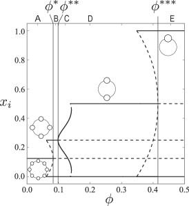
A Bifurcation diagram

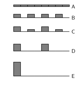
B Spatial patterns

Figure C.1: Class I model (Krugman-JPE1991)

The global dispersion force in the Krugman model stems from competition between firms over consumers’ demand. When $\phi$ is low (when transport costs are high), firms have few incentives to agglomerate, and the uniform distribution is stable. As $\phi$ increases, competition with firms in other regions becomes fiercer, as the markets of other regions become closer. At some point firms are better off forming small agglomerations so that each agglomeration has its dominant market area but is relatively remote from other agglomerations of firms. At the so-called “break point” $\phi^{*}$, a bifurcation from $\bar{\bm{x}}$ occurs and the spatial pattern is pushed towards the formation of $\frac{8}{2}=4$ distinct agglomerations [Proposition 1 (a)].

A further increase in $\phi$ causes the second and third bifurcations at $\phi^{**}$ and $\phi^{***}$, respectively. These bifurcations sequentially double the spacing between agglomerations, each time halving their number, $4\to 2\to 1$, in a close analogy to the first bifurcation at $\phi^{*}$. At the higher extreme of $\phi$, agents concentrate in a single region. This behavior can be understood as a gradual extension of the market area of each agglomeration.

In the model, agglomerations become larger when interregional access improves. However, such an effect is limited to the “selected” regions. Furthermore, as $\phi$ increases, once selected regions can decline to form an agglomeration shadow (Arthur-Book1994; Fujita-Krugman-RSUE1995) of other agglomerations. For example, consider the fifth region from the left in Figure 1B. This region attracts agents at $\phi^{*}$ and $\phi^{**}$. The impact of an increase in $\phi$ on its population is positive. After $\phi^{***}$ is encountered, it immediately loses its population. For the region, a monotonic increase in $\phi$ implies a winning situation followed by a losing one. The global dispersion force in Class I models is thus related to the rise and fall of major economic agglomerations. lp;Class I models do not provide robust predictions for each agglomeration, but they do for the overall spatial distribution of agents: the number of distinct agglomerations and spacing between them monotonically decreases and increases, respectively, with the monotonic reduction in interregional transport costs.

C.2 Class II model

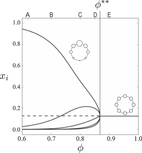
A Bifurcation diagram

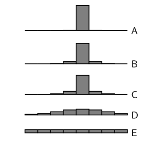
B Spatial patterns

Figure C.2: Class II model (Allen-Arkolakis-QJE2014)

Figure C.2 considers a Class II model by Allen-Arkolakis-QJE2014 (Appendix D.2.4). The model incorporates a local dispersion force but no global dispersion force. The uniform equilibrium $\bar{\bm{x}}$ is stable when transport costs are low (when $\phi$ is close to $1$). If we start from $\bar{\bm{x}}$ and consider the process of a monotonic decrease in $\phi$ from $\phi\approx 1$, then a unimodal pattern emerges due to the bifurcation at $\phi^{**}$. This is the bifurcation in the model. When $\phi$ decreases further, the spatial pattern smoothly converges to a full concentration in a single region in the lower extreme ($\phi\approx 0$). The local dispersion force is less important than the benefits of agglomeration when interregional transportation is prohibitively costly. Mobile agents prefer concentrating on a smaller number of regions because of the agglomeration forces. As $\phi$ increases, agglomeration force due to costly transportation diminishes, and the relative rise in the local dispersion force induces a crowding-out from the populated region to the adjacent regions. As a result, the spatial pattern gradually flattens and connects to $\bar{\bm{x}}$ at $\phi^{**}$.

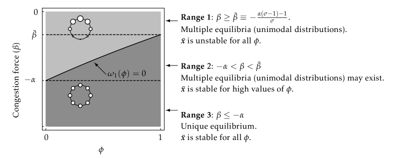
Figure C.3: Uniqueness and stability of equilibria in the Allen–Arkolakis model

We can interpret the region at the mode of population distribution (region $i$ such that $x_{i}>x_{i-1}$ and $x_{i}>x_{i+1}$ where mod $N$ for indices) as the location of an agglomeration. Then, this model endogenously produces at most one agglomeration.

Remark C.1.

In Class II models, we can ensure the uniqueness of the equilibrium regardless of the level of interregional transport costs by imposing strong local dispersion force (e.g., Redding-Sturm-AER2008; Allen-Arkolakis-QJE2014). Example 2.1 is a prototypical case in which a strong congestion force suppress endogenous agglomeration ($\gamma\geq 1$). Such uniqueness implies the stability of $\bar{\bm{x}}$ for all $\phi$ in a racetrack economy. No endogenous asymmetry can emerge, as $\bar{\bm{x}}$ is the only stable equilibrium (Assumption E is not satisfied). Figure C.3 shows the classification of possible spatial patterns and their stability for the Allen–Arkolakis model in a racetrack economy. The uniqueness condition for the model is $\beta\leq-\alpha$ (Range 3), which is a sufficient condition for the stability of $\bar{\bm{x}}$. Figure C.3 can be seen as a refinement of Figure I of Allen-Arkolakis-QJE2014 that shows endogenous spatial patterns in a circular domain. ∎

C.3 Class III model

Class III models exhibit a rich and realistic interplay between the number of agglomerations, spacing between them (as in Class I models), and the spatial extent of each agglomeration (as in Class II models).

Figure 4A shows the evolution of the number of agglomerations in the course of increasing $\phi$ under the Pfluger-Suedekum-JUE2008’s model (Appendix D.2.3). The number of agglomerations in a spatial distribution is defined by that of the local maxima therein. Figure 4A exhibits the mixed characteristics of Figures C.1 and C.2, as expected. When $\phi<\phi^{*}$ or $\phi>\phi^{**}$, $\bar{\bm{x}}$ is stable. We interpret the number of agglomerations in $\bar{\bm{x}}$ as either $8$ (for a low $\phi$) or $1$ (for a high $\phi$) to acknowledge that $\bar{\bm{x}}$ at the low and high levels of $\phi$ are distinct. When $\phi$ gradually increases from $\phi\approx 0$, the number of agglomerations reduces from $8\to 4\to 2\to 1$ as in the Class I models (Figure C.1), whereas it is always $1$ in the latter stage as per the Class II models (Figure C.2). The initial stage is governed by a decline in the global dispersion force, while the later stage is marked by a relative rise of the local dispersion force.

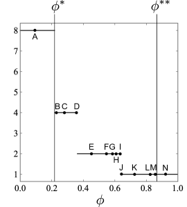
A Number of agglomerations

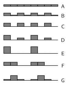
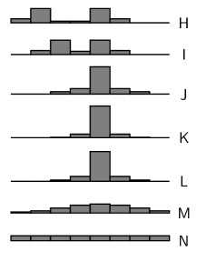
B Spatial patterns

Figure C.4: Class III model (Pfluger-Suedekum-JUE2008)

Figure 4B illustrates the spatial patterns associated with Figure 4A. Uniform pattern $\bar{\bm{x}}$ is initially stable (Pattern A) and the first bifurcation at $\phi^{*}$ leads to a quad-modal agglomeration (B, C), whereas the second bifurcation to the formation of a bimodal agglomeration (D, E). These transitions are in line with Figure C.1 and are governed by the gradual decline in the global dispersion force. A further decline in the global dispersion force increases the relative importance of the local dispersion force. As a result, the bimodal agglomeration flattens out gradually (F, G). When $\phi$ increases further, it reduces to a unimodal agglomeration (J, K). The unimodal agglomeration flattens out as $\phi$ increases (L, M) until it converges to the complete dispersion (N) at $\phi^{**}$. See also Appendix E.

Remark C.2.

In our framework, the payoff function is homogeneous across mobile agents. The effects of introducing idiosyncratic payoff shocks are of interest, since it is a standard recipe in quantitative models (Redding-Rossi-Hansberg-ARE2017). The idiosyncratic payoff shocks should act as some dispersion force without connection to the underlying geography. In fact, such idiosyncratic heterogeneity is isomorphic to a local dispersion force. For example, for additive random utility models, the idiosyncratic payoff is defined by $\hat{v}_{ni}(\bm{x})=\tilde{v}_{i}(\bm{x})+\epsilon_{ni}$ where $\tilde{v}_{i}(\bm{x})$ is the homogeneous payoff for choosing region $i$ and $\epsilon_{ni}$ is random shock drawn for each agent $n$ in region $i$. A spatial equilibrium is defined by $x_{i}=P_{i}(\bm{x})$, where $P_{i}(\bm{x})\equiv\Pr\big{(}i\in\operatornamewithlimits{arg\,max}_{j\in\mathcal{N}}\hat{v}_{nj}(\bm{x})\big{)}\in(0,1)$ is the probability for an agent to choose region $i$ when the current state is $\bm{x}$. Random utility models have deterministic interpretations (anderson1992discrete) in the sense that there is a deterministic (homogeneous) payoff function $\bm{v}(\bm{x})=(v_{i}(\bm{x}))_{i\in\mathcal{N}}$, associated with the stochastic (heterogeneous) payoff $(\hat{v}_{ni}(\bm{x}))$, such that $\bm{x}^{*}$ is a deterministic spatial equilibrium under $\bm{v}$ if and only if $x_{i}^{*}=P_{i}(\bm{x}^{*})$. Thus, the two equilibrium concepts are isomorphic in terms of the equilibrium spatial distribution of agents (Behrens-Murata-DP2018). For additive random utility models, hofbauer2007evolution demonstrates that the deterministic payoff is represented as $\bm{v}(\bm{x})=\tilde{\bm{v}}(\bm{x})-\nabla H(\bm{x})$, where $H$ is a scalar-valued function. When $\epsilon_{ni}$ is Gumbel-distributed, $H(\bm{x})=\eta\sum_{i\in\mathcal{N}}x_{i}\log x_{i}$, where $\eta$ is a constant. Thus, $v_{i}(\bm{x})=\tilde{v}_{i}(\bm{x})-\eta\log x_{i}-\eta$, implying $\mathbf{V}\propto\tilde{\mathbf{V}}-\eta\mathbf{I}$, where $\mathbf{V}$ and $\tilde{\mathbf{V}}$ are, respectively, the elasticity matrix for $\bm{v}$ and $\tilde{\bm{v}}$ at $\bar{\bm{x}}$. If $G$ and $\tilde{G}$ are the gain functions for $\bm{v}$ and $\tilde{\bm{v}}$, then $G(\chi)\propto\tilde{G}(\chi)-\eta$. Introducing payoff shocks is equivalent to adding a negative constant term (local dispersion force) to the gain function of the homogeneous component $\tilde{\bm{v}}$. As such, introducing payoff shocks to a Class I model changes the model to Class III. ∎

Appendix D Derivations for examples

This section collects derivations for $G$ and $G^{\sharp}$ for the examples in the main text. Below, $\mathbf{F}_{x}=[\frac{\partial f_{i}}{\partial x_{j}}]$ is the partial derivative (the Jacobian matrix) of a vector-valued function $\bm{f}(\bm{x})$ with respect to $\bm{x}$. For example, $\mathbf{V}_{x}\equiv[\frac{\partial v_{i}}{\partial x_{j}}]$, $\tilde{\mathbf{V}}_{w}\equiv[\frac{\partial\tilde{v}_{i}}{\partial w_{j}}]$, and $\mathbf{W}_{x}\equiv[\frac{\partial w_{i}}{\partial x_{j}}]$. They are evaluated at $\bar{\bm{x}}$ unless otherwise noted. Throughout, $\bar{v}$, $\bar{w}$, $\bar{e}$ and so on represent $v_{i}$, $w_{i}$, $e_{i}$ evaluated at $\bar{\bm{x}}$, unless otherwise noted.

D.1 General derivations of $\mathbf{V}=\frac{\bar{x}}{\bar{v}}\mathbf{V}_{x}$ and $\mathbf{A}=\frac{\bar{a}}{\bar{v}}\mathbf{V}_{a}$

D.1.1 The payoff elasticity matrix with respect to $\bm{x}$ $\mathbf{V}=\frac{\bar{x}}{\bar{v}}\mathbf{V}_{x}$

The payoff functions for the models we referenced in the main text reduce to the following form:

$$\bm{v}(\bm{x})=\tilde{\bm{v}}(\bm{x},\bm{w}),$$ (D.1)

$$\bm{s}(\bm{x},\bm{w})=\bm{0}.$$ (D.2)

The condition (D.2) represents, for example, the market equilibrium conditions for a given $\bm{x}$ that defines endogenous variable $\bm{w}$ other than $\bm{x}$ as an implicit function of $\bm{x}$. For $\bm{v}(\bm{x})$ to be well-defined, (D.2) must admit a unique solution of $\bm{w}$ for all $\bm{x}\in\mathcal{X}$. We assume this throughout the analysis. Suppose $\bm{s}$ and $\bm{v}$ are continuously differentiable. Then, we have

$$\mathbf{V}_{x}(\bm{x})=\tilde{\mathbf{V}}_{x}(\bm{x})+\tilde{\mathbf{V}}_{w}(\bm{x})\mathbf{W}_{x}(\bm{x}),$$ (D.3)

$$\mathbf{W}_{x}(\bm{x})=-\mathbf{S}_{w}(\bm{x})^{-1}\mathbf{S}_{x}(\bm{x}),$$ (D.4)

where $\mathbf{W}_{x}(\bm{x})$ is obtained by the implicit function theorem regarding (D.2).

Under Assumptions RE and S, if $\bm{x}=\bar{\bm{x}}$, $\mathbf{V}_{x}=\mathbf{S}_{w}^{-1}(\mathbf{S}_{w}\tilde{\mathbf{V}}_{x}-\tilde{\mathbf{V}}_{w}\mathbf{S}_{x})$, since all matrices commute (they are real, symmetric, and circulant at $\bar{\bm{x}}$). In the Krugman and Helpman models, $G^{\flat}(\bar{\mathbf{D}})$ arises from $\mathbf{S}_{w}$ and represents general equilibrium effects through (D.2). For any model whose payoff function reduces to the equations of the form (D.1) and (D.2), $\mathbf{V}=G^{\flat}(\bar{\mathbf{D}})^{-1}G^{\sharp}(\bar{\mathbf{D}})$ where polynomials $G^{\sharp}(\cdot)$ and $G^{\flat}(\cdot)$ are chosen such that $G^{\sharp}(\bar{\mathbf{D}})=\mathbf{S}_{w}\tilde{\mathbf{V}}_{x}-\tilde{\mathbf{V}}_{w}\mathbf{S}_{x}$ and $G^{\flat}(\bar{\mathbf{D}})=\mathbf{S}_{w}$.

Example D.1.

In Examples 3.1 and 3.2, (D.2) is given by

$$s_{i}(\bm{x},\bm{w})=w_{i}x_{i}-\sum_{j\in\mathcal{N}}m_{ij}e_{j}=0,$$ (D.5)

where $e_{i}=e(w_{i},x_{i})$ with some nonnegative function $e$ and $\mathbf{M}=\mathbf{M}(\bm{x})=[m_{ij}]$ is

$$m_{ij}=\dfrac{x_{i}w_{i}^{1-\sigma}\phi_{ij}}{\sum_{k\in\mathcal{N}}x_{k}w_{k}^{1-\sigma}\phi_{kj}}.$$ (D.6)

In matrix form, we may write (D.5) as $\bm{y}-\mathbf{M}\bm{e}=\bm{0}$ where $\bm{y}=(w_{i}x_{i})_{i\in\mathcal{N}}$. It gives

$$\mathbf{S}_{x}(\bm{x})=\operatornamewithlimits{diag}[\bm{w}]-\left(\operatornamewithlimits{diag}[\mathbf{M}\bm{e}]-\mathbf{M}\operatornamewithlimits{diag}[\bm{e}]\mathbf{M}^{\top}\right)\operatornamewithlimits{diag}[\bm{x}]^{-1}-\mathbf{M}\mathbf{E}_{x},$$ (D.7a)

$$\mathbf{S}_{w}(\bm{x})=\operatornamewithlimits{diag}[\bm{x}]+(\sigma-1)\left(\operatornamewithlimits{diag}[\mathbf{M}\bm{e}]-\mathbf{M}\operatornamewithlimits{diag}[\bm{e}]\mathbf{M}^{\top}\right)\operatornamewithlimits{diag}[\bm{w}]^{-1}-\mathbf{M}\mathbf{E}_{w}.$$ (D.7b)

Suppose Assumptions RE and S. Suppose $\bm{x}=\bar{\bm{x}}$ and let $\bar{w}$ be the uniform level of $\{w_{i}\}$ at $\bar{\bm{x}}$. We have $\mathbf{M}=\bar{\mathbf{D}}$ at $\bm{x}=\bar{\bm{x}}$. Suppose the scalars $\epsilon_{x}$ and $\epsilon_{w}$ are chosen to satisfy $\mathbf{E}_{x}=\epsilon_{x}\bar{w}\mathbf{I}$ and $\mathbf{E}_{w}=\epsilon_{w}\bar{x}\mathbf{I}$ at $\bar{\bm{x}}$. Let $\bar{e}=e(\bar{w},\bar{x})$ and $\zeta\equiv\frac{\bar{e}}{\bar{w}\bar{x}}$. We see that

$$\mathbf{S}_{x}=-\bar{w}\left((\zeta-1)\mathbf{I}+\epsilon_{x}\bar{\mathbf{D}}-\zeta\bar{\mathbf{D}}^{2}\right),$$ (D.8a)

$$\mathbf{S}_{w}=\bar{x}\left(\left(1+\zeta(\sigma-1)\right)\mathbf{I}-\epsilon_{w}\bar{\mathbf{D}}-\zeta(\sigma-1)\bar{\mathbf{D}}^{2}\right).$$ (D.8b)

If $e(w_{i},x_{i})=w_{i}x_{i}$, then $\epsilon_{x}=\epsilon_{w}=1$ and $\zeta=1$, thereby $\mathbf{W}_{x}=\frac{\bar{w}}{\bar{x}}(\sigma\mathbf{I}+(\sigma-1)\bar{\mathbf{D}})^{-1}\bar{\mathbf{D}}$. ∎

D.1.2 The payoff elasticity matrix with respect to $\bm{a}$ $\mathbf{A}=\frac{\bar{x}}{\bar{a}}\mathbf{V}_{a}$

In (B.14), $\mathbf{X}=[\partial x_{i}(\bar{\bm{a}})/\partial a_{i}]=\mathbf{X}_{a}$ acts as $\hat{\mathbf{X}}\equiv-\mathbf{V}_{x}^{-1}\mathbf{V}_{a}$ for $\bm{z}$ such that $\bm{z}^{\top}\bm{1}=\bm{0}$. Thus, $\mathbf{V}_{a}$ is of interest.

For purely local characteristics (Example 5.1), since $v_{i}(\bm{x},\bm{a})=a_{i}v_{i}(\bm{x})$, it follows that $\mathbf{V}_{a}=\operatornamewithlimits{diag}[\bm{v}(\bm{x})]$. At $\bar{\bm{x}}$, we have $\mathbf{V}_{a}=\bar{v}\mathbf{I}$. Thus, $\hat{\mathbf{X}}=-\bar{v}\mathbf{V}_{x}^{-1}$.

For regional characteristics that affect trade flows (Examples 5.6 and 5.5), the payoff function and the market equilibrium condition are, respectively, modified to $\bm{v}(\bm{x},\bm{a})=\tilde{\bm{v}}(\bm{x},\bm{w},\bm{a})$ and $\bm{s}(\bm{x},\bm{w},\bm{a})=\bm{0}$. By applying the implicit function theorem, we see $\mathbf{V}_{a}=\tilde{\mathbf{V}}_{a}+\tilde{\mathbf{V}}_{w}\mathbf{W}_{a}=\tilde{\mathbf{V}}_{a}-\tilde{\mathbf{V}}_{w}\mathbf{S}_{w}^{-1}\mathbf{S}_{a}$. As all matrices commute at $\bar{\bm{x}}$ under Assumptions RE and S, it is equivalent to consider

$$\hat{\mathbf{X}} =-\left(\tilde{\mathbf{V}}_{x}-\tilde{\mathbf{V}}_{w}\mathbf{S}_{w}^{-1}\mathbf{S}_{x}\right)^{-1}\left(\tilde{\mathbf{V}}_{a}-\tilde{\mathbf{V}}_{w}\mathbf{S}_{w}^{-1}\mathbf{S}_{a}\right)$$ (D.9)

$$=\left(\mathbf{S}_{w}\tilde{\mathbf{V}}_{x}-\tilde{\mathbf{V}}_{w}\mathbf{S}_{x}\right)^{-1}\left(\tilde{\mathbf{V}}_{w}\mathbf{S}_{a}-\mathbf{S}_{w}\tilde{\mathbf{V}}_{a}\right).$$ (D.10)

Example D.2.

In Example 5.6, we have

$$s_{i}(\bm{x},\bm{w},\bm{a})=w_{i}x_{i}-\sum_{j\in\mathcal{N}}\dfrac{x_{i}a_{i}w_{i}^{1-\sigma}\phi_{ij}}{\sum_{k\in\mathcal{N}}x_{k}a_{k}w_{k}^{1-\sigma}\phi_{kj}}e_{j}=0.$$ (D.11)

So, $\mathbf{S}_{a}=-\left(\operatornamewithlimits{diag}[\mathbf{M}\bm{e}]-\mathbf{M}\operatornamewithlimits{diag}[\bm{e}]\mathbf{M}^{\top}\right)\operatornamewithlimits{diag}[\bm{a}]^{-1}=-\frac{\bar{e}}{\bar{a}}\left(\mathbf{I}-\bar{\mathbf{D}}^{2}\right)$. See Appendix D.2.2. ∎

Example D.3.

In Example 5.5, we have

$$s_{i}(\bm{x},\bm{w},\bm{a})=w_{i}x_{i}-\sum_{j\in\mathcal{N}}\dfrac{x_{i}w_{i}^{1-\sigma}\phi_{ij}}{\sum_{k\in\mathcal{N}}x_{k}w_{k}^{1-\sigma}\phi_{kj}}e(w_{j},x_{j},a_{j})=0$$ (D.12)

where $e$ maps the tuple $(w_{j},x_{j},a_{j})$ to the regional expenditure. Then, we have $\mathbf{S}_{a}=-\mathbf{M}\mathbf{E}_{a}$, or $\mathbf{S}_{a}=-\epsilon_{a}\bar{\mathbf{D}}$ at $\bar{\bm{x}}$ where $\epsilon_{a}=\frac{\partial e(\bar{x},\bar{w},\bar{a})}{\partial a_{i}}$. See Appendix D.2.1. ∎

D.2 Model-specific derivations of $\mathbf{V}=\frac{\bar{x}}{\bar{v}}\mathbf{V}_{x}$

We provide omitted derivations of the gain functions $G$ for the main examples. See Akamatsu-et-al-DP2017 for derivations for other models in Examples 3.3, 3.4, and 3.5.

D.2.1 Krugman-JPE1991 model (Examples 3.1 and 5.5)

There are two types of workers, mobile and immobile, and their total masses are $1$ and $L$, respectively. $\bm{x}\equiv(x_{i})_{i\in\mathcal{N}}$ is the distribution of mobile workers. Each worker supplies one unit of labor inelastically.

There are two industrial sectors: agriculture (abbreviated as A) and manufacturing (abbreviated as M). The A-sector is perfectly competitive and a unit input of immobile labor is required to produce one unit of goods. The M-sector follows Dixit–Stiglitz monopolistic competition. M-sector goods are horizontally differentiated and produced under increasing returns to scale using mobile labor as the input. The goods of both sectors are transported. Transportation of A-sector goods is frictionless, while that of M-sector goods is of an iceberg form. For each unit of M-sector goods transported from region $i$ to $j$, only the proportion $1/\tau_{ij}$ arrives, where $\tau_{ij}>1$ for $i\neq j$ and $\tau_{ii}=1$.

All workers have an identical preference for both M- and A-sector goods. The utility of a worker in region $i$ is given by a two-tier form. The upper tier is Cobb–Douglas over the consumption of A-sector goods $C_{i}^{\mathrm{A}}$ and that of M-sector constant-elasticity-of-substitution (CES) aggregate $C_{i}^{\mathrm{M}}$ with $\sigma>1$

$$C_{i}^{\mathrm{M}}\equiv\Big{(}\sum_{j\in\mathcal{N}}\int_{0}^{n_{j}}q_{ji}(\xi)^{\frac{\sigma-1}{\sigma}}\mathrm{d}\xi\Big{)}^{\frac{\sigma}{\sigma-1}},$$ (D.13)

that is, $u_{i}=(C_{i}^{\mathrm{A}})^{\mu}(C_{i}^{\mathrm{A}})^{1-\mu}$ where $\mu\in(0,1)$ is the constant expenditure of the latter. With free trade in the A-sector, the wage of the immobile worker is equalized, and we normalize it to unity by taking A-sector goods as the numéraire. Consequently, region $i$’s expenditure on the M-sector goods is given by $e_{i}=\mu(w_{i}x_{i}+l_{i})$ where $l_{i}$ denotes the mass of immobile workers in region $i$.

In the M-sector, to produce $q$ units, a firm requires $\alpha+\beta q$ units of mobile labor. Profit maximization of firms yields the price of differentiated goods produced in region $i$ and exported to $j$ as $p_{ij}=\frac{\sigma\beta}{\sigma-1}w_{i}\tau_{ij}$, which in turn determines gravity trade flow from $j$ to $i$. That is, when $X_{ij}$ denotes the price of M-sector goods produced in region $i$ and sold in region $j$, $X_{ij}=m_{ij}e_{j}$ where the share $m_{ij}\in(0,1)$ is defined by (D.6) with $\phi_{ij}\equiv\tau_{ij}^{1-\sigma}$. The proximity matrix is thus $\mathbf{D}=[\phi_{ij}]=[\tau_{ij}^{1-\sigma}]$.

Given $\bm{x}$, we determine the market wage $\bm{w}\equiv(w_{i})_{i\in\mathcal{N}}$ by the M-sector product market-clearing, zero-profit, and mobile labor market-clearing conditions. These conditions are summarized by the trade balance $w_{i}x_{i}=\sum_{j\in\mathcal{N}}X_{ij}$, or (D.5) with $e(x_{i},w_{i})=\mu(w_{i}x_{i}+l_{i})$. By adding up (D.5) for the Krugman model, we see $\sum_{i\in\mathcal{N}}w_{i}x_{i}=\frac{\mu}{1-\mu}L$, which constrains the total income of mobile workers at any configuration $\bm{x}$. The existence and uniqueness of the solution for (D.5) follow from standard arguments (e.g., Facchinei-Pang-Book2007). Given the solution $\bm{w}(\bm{x})$ of (D.5), we have the indirect utility of mobile workers, which is given by $v_{i}=\Delta_{i}^{\frac{\mu}{\sigma-1}}w_{i}$, where $\Delta_{i}\equiv\sum_{k\in\mathcal{N}}x_{k}w_{k}^{1-\sigma}d_{ki}$.

To satisfy Assumption S, let $l_{i}=l\equiv\frac{L}{N}$ for all $i\in\mathcal{N}$. We have

$$\nabla\log\bm{v}(\bar{\bm{x}}) =\dfrac{\mu}{\sigma-1}\mathbf{M}^{\top}\operatornamewithlimits{diag}[\bm{x}]^{-1}-\mu\mathbf{M}^{\top}\operatornamewithlimits{diag}[\bm{w}]^{-1}\mathbf{W}_{x}+\operatornamewithlimits{diag}[\bm{w}]^{-1}\mathbf{W}_{x}$$ (D.14)

$$=\frac{1}{\bar{x}}\dfrac{\mu}{\sigma-1}\bar{\mathbf{D}}+\frac{1}{\bar{w}}\left(\mathbf{I}-\mu\bar{\mathbf{D}}\right)\mathbf{W}_{x},$$ (D.15)

where (D.4) and (D.8) give $\mathbf{W}_{x}$. By plugging $\delta=\frac{\mu(\bar{w}\bar{x}+l)}{\bar{w}\bar{x}}=1$ and $\epsilon_{x}=\epsilon_{w}=\mu$ to (D.8),

$$\mathbf{W}_{x}=\dfrac{\bar{w}}{\bar{x}}\left(\sigma\mathbf{I}-\mu\bar{\mathbf{D}}-(\sigma-1)\bar{\mathbf{D}}^{2}\right)^{-1}\left(\mu\bar{\mathbf{D}}-\bar{\mathbf{D}}^{2}\right).$$ (D.16)

Then, (D.15) and (D.16) imply

$$\mathbf{V}=\bar{x}\nabla\log\bm{v}(\bar{\bm{x}})=\frac{\mu}{\sigma-1}\bar{\mathbf{D}}+\left(\mathbf{I}-\mu\bar{\mathbf{D}}\right)\left(\sigma\mathbf{I}-\mu\bar{\mathbf{D}}-(\sigma-1)\bar{\mathbf{D}}^{2}\right)^{-1}\left(\mu\bar{\mathbf{D}}-\bar{\mathbf{D}}^{2}\right),$$ (D.17)

or equivalently, $\mathbf{V}=G(\bar{\mathbf{D}})$ where

$$G(\chi) =\underbrace{\frac{\mu}{\sigma-1}\chi}_{\text{(a)}}+\underbrace{(1-\mu\chi)}_{\text{(b)}}\underbrace{\left(\frac{1}{\sigma}\right)\frac{\mu\chi-\chi^{2}}{1-\frac{\mu}{\sigma}\chi-\frac{\sigma-1}{\sigma}\chi^{2}}}_{\text{(c)}}.$$ (D.18)

From (D.18) we have $\mathbf{V}=G^{\flat}(\bar{\mathbf{D}})^{-1}G^{\sharp}(\bar{\mathbf{D}})$, where we define

$$G^{\sharp}(\chi)\equiv\mu\left(\dfrac{1}{\sigma-1}+\dfrac{1}{\sigma}\right)\chi-\left(\dfrac{\mu^{2}}{\sigma-1}+\dfrac{1}{\sigma}\right)\chi^{2},$$ (D.19)

$$G^{\flat}(\chi)\equiv 1-\frac{\mu}{\sigma}\chi-\frac{\sigma-1}{\sigma}\chi^{2}.$$ (D.20)

Remark D.1.

Using the Krugman model as an example, we discuss how economic forces in a model are embedded in $G$ and $G^{\sharp}$. We recall that positive (negative) terms in $G$ represent agglomeration (dispersion) forces (Definition 2). In (D.18), (a) corresponds to the elasticity of price index with respect to agents’ spatial distribution $\bm{x}$, (b) to the elasticity of payoff with respect to nominal wage $\bm{w}$, (c) to the elasticity of wage with respect to agents’ spatial distribution. Here, (a) and the second term in (b) corresponds to the so-called cost-of-living effect through price index; (a) is positive, i.e., it is an agglomeration force, as the price index in a region becomes lower when more agents (firms) locate geographically close regions; the second term in (b) (i.e., $-\mu\chi$) is negative because higher wage in a region implies higher goods prices in its nearby regions. Also, (b) as a whole is positive, meaning that the payoff of a region is increasing in wages even with the negative effect through price index. The last component (c) includes both positive and negative terms; in its numerator, the first term ($\mu\chi$) is demand linkage where firms’ profits rise when they are close to regions with high total income, and the second term ($-\chi^{2}$) is the market-crowding effect due to competition between firms. The sign of (c) is $\chi$-dependent; for example, it is negative when $\chi$ is high ($\phi$ is low) and positive otherwise. The denominator of (c) represents the general equilibrium effects through the so-called short-run equilibrium condition under given $\bm{x}$, i.e., (D.5). As $G^{\sharp}$ is obtained by combining these components and collecting terms according to the order of $\chi$, these economic forces affect both the first- and second-order coefficients of $G^{\sharp}$. Concretely, in (D.19), $\frac{\mu}{\sigma-1}\chi$ comes from (a), $\frac{\mu}{\sigma}\chi$ comes from (b) $\times$ (c), $-\frac{1}{\sigma}\chi^{2}$ comes from (b) $\times$ (c), and $-\frac{\mu^{2}}{\sigma-1}\chi^{2}=-\left(\frac{\mu^{2}}{\sigma}+\frac{\mu^{2}}{\sigma(\sigma-1)}\right)\chi^{2}$ comes from all three components while its leading term $-\frac{\mu^{2}}{\sigma}\chi^{2}$ comes from (b) $\times$ (c). Thus, by considering $G^{\sharp}$ for a model, one can examine the net effect of all economic forces in the model at once, and the net effect is decomposed according to its spatial scale (i.e., the order of $\chi$). ∎

Remark D.2.

In Figure C.1, we set $\mu=0.5$, $\sigma=10$, and $L=8$. ∎

Remark D.3 (Example 5.5).

To obtain $G^{\natural}$ for $\bm{l}=(l_{i})_{i\in\mathcal{N}}$, we evaluate $\mathbf{V}_{l}=-\tilde{\mathbf{V}}_{w}\mathbf{S}_{w}^{-1}\mathbf{S}_{l}$ as $\mathbf{A}=\frac{l}{\bar{v}}\mathbf{V}_{l}$. From Example D.3, $\mathbf{S}_{l}=-\mu\bar{\mathbf{D}}$. Also, $\tilde{\mathbf{V}}_{w}=\bar{v}\frac{\partial}{\partial\bm{w}}\log\bm{v}(\bar{\bm{x}})=\frac{\bar{v}}{\bar{w}}(\mathbf{I}-\mu\bar{\mathbf{D}})$ and $\tilde{\mathbf{V}}_{l}=\bm{0}$. Thus,

$$G^{\natural}(\chi)=c\frac{\chi(1-\mu\chi)}{G^{\flat}(\chi)}>0$$ (D.21)

where $c=\frac{l}{\bar{w}}\frac{\mu}{\sigma}=\frac{1-\mu}{\sigma}\bar{x}>0$. It then follows that

$$\delta(\chi)=-\frac{\bar{x}}{\bar{a}}\frac{G^{\natural}(\chi)}{G(\chi)}=-\frac{c\bar{x}}{\bar{a}}\frac{\chi(1-\mu\chi)}{G^{\sharp}(\chi)}.$$ (D.22)

Straightforward algebra verifies that $\delta^{\prime}(\chi)<0$ if $G^{\sharp}(\chi)>0$. ∎

D.2.2 Helpman-Book1998 model (Examples 3.2 and 5.6)

Helpman-Book1998 removed the A-sector in the Krugman model and assumed that all workers are mobile. Instead of the A-sector, the model introduces the housing (abbreviated as H) sector. Each region $i$ is endowed with a fixed stock $a_{i}$ of housing. Workers’ preference is Cobb–Douglas of M-sector CES aggregate $C_{i}^{\mathrm{M}}$ and H-sector goods $C_{i}^{\mathrm{H}}$, $u_{i}=(C_{i}^{\mathrm{M}})^{\mu}(C_{i}^{\mathrm{H}})^{\gamma}$, where $\mu\in(0,1)$ is the expenditure share of the former and $\gamma=1-\mu\in(0,1)$ is that for the latter. There are two variants for assumptions on how housing stocks are owned: public landownership (abbreviated as PL) and local landownership (LL). The original formulation by Helpman-Book1998 supposes housing stocks are equally owned by all workers (i.e., PL). The income of a worker in region $i$ is the sum of the wage and an equal dividend $r>0$ of rental revenue over the economy. However, ottaviano2002agglomeration, Murata-Thisse-JUE2005, and Redding-Sturm-AER2008 assumed that housing stocks are locally owned (i.e., LL). The income of a worker in region $i$ is the sum of the wage and an equal dividend of rental revenue in each region.

Regarding the market equilibrium conditions, the only difference from the Krugman model is regional expenditure $e_{i}$ on M-sector goods in each region:

[PL] $$e_{i}=\mu\left(w_{i}+r\right)x_{i},$$ (D.23)

[LL] $$e_{i}=w_{i}x_{i}.$$ (D.24)

Also, the arket wage is given as the solution for (D.5). For the PL case, we set $r=1$ for normalization. For the LL case, $\bm{w}(\bm{x})$ is uniquely given up to normalization. The indirect utility function is, with $\Delta_{i}\equiv\sum_{j\in\mathcal{N}}x_{j}w_{j}^{1-\sigma}\phi_{ji}$ and $r>0$,

[PL] $$v_{i}=\left(\frac{x_{i}}{a_{i}}\right)^{-\gamma}(w_{i}+r)^{\mu}\Delta_{i}^{\frac{\mu}{\sigma-1}},$$ (D.25)

[LL] $$v_{i}=\left(\frac{x_{i}}{a_{i}}\right)^{-\gamma}w_{i}^{\mu}\Delta_{i}^{\frac{\mu}{\sigma-1}}.$$ (D.26)

Let $a_{i}=1$ to satisfy Assumption S. We compute that

$$\mathbf{V}=\bar{x}\left(\frac{\mu}{\sigma-1}\mathbf{M}^{\top}\operatornamewithlimits{diag}[\bm{x}]^{-1}+\hat{\mathbf{V}}_{w}\mathbf{W}_{x}-\gamma\operatornamewithlimits{diag}[\bm{x}]^{-1}\right),$$ (D.27)

where $$\text{[PL]}\quad\hat{\mathbf{V}}_{w}\equiv\mu\left(\operatornamewithlimits{diag}[\bm{w}+r\bm{1}]^{-1}-\mathbf{M}^{\top}\operatornamewithlimits{diag}[\bm{w}]^{-1}\right),$$ (D.28)

$$\text{[LL]}\quad\hat{\mathbf{V}}_{w}\equiv\mu\left(\mathbf{I}-\mathbf{M}^{\top}\right)\operatornamewithlimits{diag}[\bm{w}]^{-1},$$ (D.29)

and $\mathbf{M}$ is defined by (D.6). For the PL case, we obtain $\mathbf{V}=G(\bar{\mathbf{D}})$ with

$$G(\chi)=-\gamma+\frac{\mu}{\sigma-1}\chi+\frac{\mu\left(\mu-\chi\right)\chi(1-\chi)}{\sigma-\mu\chi-(\sigma-1)\chi^{2}}$$ (D.30)

where we compute $\mathbf{W}_{x}$ from (D.7) with $\zeta=\frac{\mu(\bar{w}+1)}{\bar{w}}$, $\epsilon_{x}=\frac{\bar{w}+1}{\bar{w}}$, $\epsilon_{w}=\mu$; we note that $\frac{\bar{w}}{\bar{w}+1}=\mu$ under our normalization. Thus, for the PL case, we can choose $G^{\sharp}$ and $G^{\flat}$ that satisfy $\mathbf{V}=G^{\flat}(\bar{\mathbf{D}})^{-1}G^{\sharp}(\bar{\mathbf{D}})$ as follows:

$$G^{\sharp}(\chi)\equiv-\gamma+\left(\frac{\mu}{\sigma-1}+\dfrac{\mu(\mu+\gamma)}{\sigma}\right)\chi-\left(\frac{\mu^{2}}{\sigma-1}+\dfrac{\mu+\gamma}{\sigma}-\gamma\right)\chi^{2},$$ (D.31)

$$G^{\flat}(\chi)\equiv 1-\dfrac{\mu}{\sigma}\chi-\dfrac{\sigma-1}{\sigma}\chi^{2}$$ (D.32)

where we recall $\mu+\gamma=1$.

Remark D.4.

As in the Krugman model (Remark D.1), one can identify the correspondence between the coefficients in $G$ (D.31) and those in $G^{\sharp}$ (D.30). For example, local dispersion force $-\gamma$ in (D.30) affects not only constant term in $G^{\sharp}(\cdot)$ but also the first- and the second-order terms of $\chi$. Other forces can be understood similarly to the Krugman model (Remark D.1). ∎

For the LL case, $\mathbf{W}_{x}$ is given in Example D.1 and we obtain

$$G(\chi)=-\gamma+\frac{\mu}{\sigma-1}\chi+\frac{\mu(1-\chi)\chi}{\sigma+(\sigma-1)\chi}.$$ (D.33)

We can choose $G^{\sharp}$ and $G^{\flat}$ as follows:

$$G^{\sharp}(\chi)\equiv-\gamma+\left(\frac{\mu}{\sigma-1}+\frac{\mu+\gamma}{\sigma}-\gamma\right)\chi,$$ (D.34)

$$G^{\flat}(\chi)\equiv 1+\dfrac{\sigma-1}{\sigma}\chi.$$ (D.35)

Remark D.5.

Equilibrium is unique when $\gamma\sigma=(1-\mu)\sigma>1$ (Redding-Sturm-AER2008). For both PL and LL, it implies that $G^{\sharp}(\chi)<0$ for all $\chi\in(0,1)$. ∎

Remark D.6 (Example 5.6).

The regional model in §3 of Redding-Rossi-Hansberg-ARE2017 is a variant of the Helpman model with LL, in which variable input of mobile labor depends on region $i$ (i.e., productivity differs across regions). The cost function of firms in region $i$ is $C_{i}(q)=w_{i}(\alpha+\beta_{i}q)$. The market equilibrium condition for this case is, with $a_{i}\equiv\beta_{i}^{1-\sigma}>0$, given by

$$s_{i}(\bm{x},\bm{w})=w_{i}x_{i}-\sum_{j\in\mathcal{N}}\dfrac{x_{i}a_{i}w_{i}^{1-\sigma}\phi_{ij}}{\sum_{k\in\mathcal{N}}x_{k}a_{k}w_{k}^{1-\sigma}\phi_{kj}}w_{j}x_{j}=0.$$ (D.36)

The payoff function is given by (D.29) with $\Delta_{i}=\sum_{k\in\mathcal{N}}x_{k}a_{k}w_{k}^{1-\sigma}\phi_{ki}$.

From Example D.2, $\mathbf{S}_{a}=-\frac{\bar{w}\bar{x}}{\bar{a}}\left(\mathbf{I}-\bar{\mathbf{D}}\right)\left(\mathbf{I}+\bar{\mathbf{D}}\right)$ as $\bar{e}=\bar{w}\bar{x}$. Also, we have $\tilde{\mathbf{V}}_{w}=\frac{\bar{v}}{\bar{w}}\mu(\mathbf{I}-\bar{\mathbf{D}})$, $\tilde{\mathbf{V}}_{a}=\frac{\bar{v}}{\bar{a}}\frac{\mu}{\sigma-1}\bar{\mathbf{D}}$, and $\mathbf{S}_{w}=\sigma\bar{x}G^{\flat}(\bar{\mathbf{D}})$. As $\mathbf{V}_{a}=\tilde{\mathbf{V}}_{a}-\tilde{\mathbf{V}}_{w}\mathbf{S}_{w}^{-1}\mathbf{S}_{a}$ and $\mathbf{A}=\frac{\bar{a}}{\bar{v}}\mathbf{V}_{a}=G^{\natural}(\bar{\mathbf{D}})$, we compute

$$G^{\natural}(\chi)=c\frac{(\sigma-1)+\sigma\chi}{G^{\flat}(\chi)}>0$$ (D.37)

where $c\equiv\frac{\bar{v}}{\bar{a}}\frac{\mu}{\sigma}>0$. This in turn implies

$$\delta(\chi)=-\frac{\bar{x}}{\bar{a}}\frac{G^{\natural}(\chi)}{G(\chi)}=-\frac{c\bar{x}}{\bar{a}}\frac{(\sigma-1)+\sigma\chi}{G^{\sharp}(\chi)}$$ (D.38)

where $G^{\sharp}(\chi)$ is that for the LL case (D.35). We have $\delta^{\prime}(\chi)>0$ for all $\chi$ whenever $(1-\mu)\sigma>1$. ∎

D.2.3 Pfluger-Suedekum-JUE2008 model (Example 3.5)

The Pflüger–Südekum model builds on Pfluger-RSUE2003 and introduces the housing sector (again denoted by H). In this model, a quasi-linear upper-tier utility is assumed: $u_{i}=C_{i}^{\mathrm{A}}+\mu\log C_{i}^{\mathrm{M}}+\gamma\log C_{i}^{\mathrm{H}}$. The production cost for a firm in $i\in\mathcal{N}$ is $\alpha w_{i}+\beta q$. Then, $\bm{w}$ is given as follows:

$$w_{i}=\dfrac{\mu}{\sigma}\sum_{j\in\mathcal{N}}\dfrac{\phi_{ij}}{\sum_{k\in\mathcal{N}}\phi_{kj}x_{k}}(x_{j}+l_{j}).$$ (D.39)

The indirect utility of a mobile worker in region $i$ is

$$v_{i}(\bm{x})=\frac{\mu}{\sigma-1}\ln[\Delta_{i}]-\gamma\ln\frac{x_{i}+l_{i}}{a_{i}}+w_{i},$$ (D.40)

where $\Delta_{i}=\sum_{j\in\mathcal{N}}\phi_{ji}x_{j}$, and $l_{i}$ and $a_{i}$ denote the mass of immobile workers and amount of housing stock in region $i$, respectively. The nominal wage in region $i$ is given by (D.39). Let $l_{i}=l$ and $a_{i}=a$ for all $i$ to meet Assumption S. Then, we see that $\mathbf{V}=\frac{1}{\bar{v}}G^{\sharp}(\bar{\mathbf{D}})$ with

$$G^{\sharp}(\chi) =-\dfrac{\gamma}{1+L}+\mu\left(\frac{1}{\sigma-1}+\frac{1}{\sigma}\right)\chi-\frac{\mu}{\sigma}(1+L)\chi^{2}.$$ (D.41)

Remark D.7.

In Figures 4A and 4B, $\mu=0.4$, $\sigma=2.5$, $L=4$, $\gamma=0.5$, and $a_{i}=1$. ∎

D.2.4 Allen-Arkolakis-QJE2014 (AA) (Example 3.4)

The AA model is a perfectly competitive Armington-IMF1969-based framework with positive and negative local externalities. We consider a discrete-space version of the model and abstract away all exogenous differences across regions. In the model, productivity of a location is proportional to $x_{i}^{\alpha}$ with $\alpha>0$, representing positive externalities. The market equilibrium condition is

$$s_{i}(\bm{x},\bm{w})=w_{i}x_{i}-\sum_{j\in\mathcal{N}}\dfrac{w_{i}^{1-\sigma}x_{i}^{\alpha(\sigma-1)}\phi_{ij}}{\sum_{k\in\mathcal{N}}w_{k}^{1-\sigma}x_{k}^{\alpha(\sigma-1)}\phi_{kj}}w_{j}x_{j}=0.$$ (D.42)

With market wage $\bm{w}$, we have $v_{i}(\bm{x})=x_{i}^{\beta}w_{i}\Delta_{i}^{\frac{1}{\sigma-1}}$ with $\Delta_{i}\equiv\sum_{k\in\mathcal{N}}w_{k}^{1-\sigma}x_{k}^{\alpha(\sigma-1)}\phi_{ki}$; $x_{i}^{\beta}$ ($\beta<0$) represents negative externalities from congestion. We have $\mathbf{V}=G^{\flat}(\bar{\mathbf{D}})^{-1}G^{\sharp}(\bar{\mathbf{D}})$ with

$$G^{\sharp}(\chi)=-\left(\alpha+\beta-\frac{1+\alpha}{\sigma}\right)+\left(\alpha+\beta+\frac{1-\beta}{\sigma}\right)\chi,$$ (D.43)

$$G^{\flat}(\chi)=\left(\sigma+(\sigma-1)\chi\right)\left(1-\chi\right).$$ (D.44)

Remark D.8.

In Figure C.2, we set $(\alpha,\beta,\sigma)=(0.5,-0.3,6)$. ∎

Appendix E Geographical advantages

This appendix illustrates that the implications of Proposition 1 qualitatively generalize to various geographical setups (one-dimensional line segment, two-dimensional spaces with/without boundaries). In particular, it is demonstrated that the spatial distribution of agents become multimodal in Class I models, whereas it becomes unimodal in Class II models, even when we relax Assumption RE.

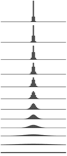
A The Helpman model (Class II)

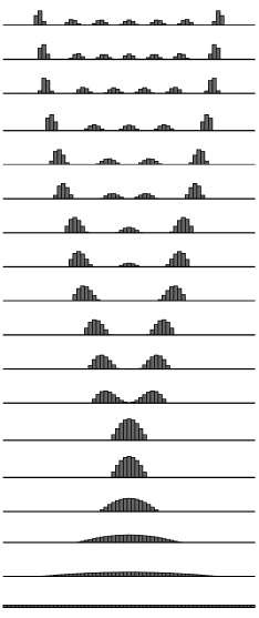
B The Pflüger–Südekum model (Class III)

Figure E.1: Stable spatial patterns for Classes II and III in a line segment (number of regions $N=65$). All regions share the same local parameters. The transport cost between every consecutive pair of regions is uniform. The level of transport cost monotonically decreases from top to bottom. For an extensive discussion on the behavior of a Class I model in a line segment, see Ikeda-et-al-IJET2017.

The simplest way to introduce geographical asymmetry into our one-dimensional setup is to consider a bounded line segment, which is a standard spatial setting in urban economic theory. Ikeda-et-al-IJET2017 considered a Class I model (Forslid-Ottaviano-JoEG2003) in a line segment. The study showed that multiple agglomerations emerge as in the racetrack economy and demonstrated that the evolution of spatial structure in a line segment approximately follows the “period doubling” behavior discussed in Section C.1. For Class II and III, Figure E.1 reports examples of endogenous agglomeration patterns in the Helpman and Pflüger–Südekum models. For both models, qualitative properties of the spatial patterns are consistent with those discussed in Appendix C.

The real-world geography is two-dimensional. The two-dimensional counterpart of the racetrack economy is bounded lattices with periodic boundary conditions (i.e., flat torus), for which a basic theory of spatial agglomeration is provided in Ikeda-Murota-Book2014. For Class I models, it is now understood that they engender multiple disjointed agglomerations and period-doubling behavior emerge from the model, as in the racetrack setup studied in this paper. As concrete examples, Figure E.2 shows endogenous equilibrium spatial patterns over a bounded square economy with $9\times 9=81$ regions in the course of increasing $\phi$ for the Krugman and Allen–Arkolakis models. The parameters are the same as Figure C.1 and Figure C.2. The Krugman model (Class I) engenders multiple disjointed agglomerations. When $\phi$ increases, the number of agglomerations gradually decreases while the spacing between them enlarges. For the AA model (Class II), in contrast, the spatial pattern is initially unimodal. As $\phi$ increases, it gradually flattens to exhibit suburbanization. All these behaviors are qualitatively consistent with Proposition 1 and examples in Appendix C, suggesting the robustness of qualitative implications of our theoretical developments.

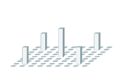
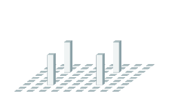
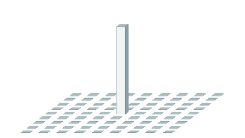
A The Krugman model (Class I)

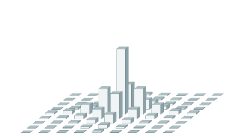
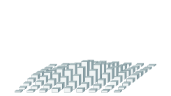
B The Allen–Arkolakis model (Class II)

Figure E.2: Stable spatial patterns in a square economy ($N=9^{2}=81$).

Remark E.1.

The implications of Proposition 1 seem to extend to different assumptions on transport technology that are not formally covered by our multiplicative specification of $\mathbf{D}$ in Assumption RE. For example, consider the models by Mossay-Picard-JET2011; Picard-Tabuchi-JET2013; Blanchet-et-al-IER2016, all of which assume linear transport technology. Mossay-Picard-JET2011 considered a variant of the Beckmann model (Class II) and showed that the only possible equilibrium is a unimodal distribution in a continuous line segment. Blanchet-et-al-IER2016 considered a general Class II model over a continuous one- or two-dimensional space; they showed that the equilibrium spatial pattern for the Beckmann model is unique and given by a regular concave paraboloid, i.e., a unimodal pattern. Picard-Tabuchi-JET2013 also considered a Class II general equilibrium model in a two-dimensional space and showed that spatial distribution becomes unimodal. For more complicated examples, the numerical results of anas1996general and anas1998urban in line segments bear a close resemblance to, respectively, agglomeration behaviors of Class I and II models, although they assume endogenous transport costs between locations. These examples highlight the utility of distinguishing local and global dispersion forces. ∎

Remark E.2.

Our observations in this section are consistent with findings in mathematics of pattern formation (see, e.g., kondo2010reaction, for a survey). From a broader scientific perspective, the racetrack setting (one-dimensional space with periodic boundary conditions) is a standard starting point of theoretical analysis of pattern formation phenomena (as initiated by Turing-PTB1953). In particular, the properties of stable spatial patterns under a model in symmetric settings qualitatively generalize to asymmetric settings (e.g., arcuri1986pattern) in the sense that if a model produces multimodal spatial patterns on the circular domain, then the model is capable of producing multimodal spatial patterns on asymmetric domains. Further, a basic requirement for the formation of stable multimodal spatial patterns is the existence of short-range positive feedback combined with long-range negative feedback for a concentration of mobile factors (meinhardt2000pattern). In our paper, global dispersion forces correspond to long-range negative feedback. ∎

Appendix F Local advantages

This section provides numerical examples for Proposition 2 for the $N=8$ case. As in Example 5.1, we multiply the payoff in region $1$ by $a_{1}\geq 1$, whereas we let $a_{i}=1$ for all $i\neq 1$. We consider the Krugman and Allen–Arkolakis (AA) models and basic model parameters to be the same as Figure C.1 and Figure C.2 except that region $1$ has an exogenous advantage.

Figure 1A reports the evolutionary paths of $x_{1}$ for the AA model (Class II) under the uniqueness of the equilibrium. The curves depict region $1$’s population share, $x_{1}$, at stable equilibria against $\phi$. Four incremental settings $a_{1}\in\{1.000,1.001,1.005,1.010\}$ are considered, including the baseline case with no location-fixed advantage ($a_{1}=1.000$). We have $\delta^{\prime}(\chi)>0$ for all $\chi\in(0,1)$ and see that $x_{1}-\bar{x}>0$ when $a_{1}>1$ and $x_{1}-\bar{x}$ increases as $a_{1}$ increases, which are intuitive. Additionally, $x_{1}-\bar{x}$ decreases as $\phi$ increases. We confirm that $\rho(\phi)>0$ and $\rho^{\prime}(\phi)<0$ for all $\phi$.

Similarly, Figure 1B and Figure 1C consider, respectively, the Krugman and AA models under a multiplicity of equilibria. Unlike the AA model, the Krugman model admits multiple equilibria for some $\phi$ for any pair of the structural parameters $(\mu,\sigma)$. Proposition 2 correctly predicts the sign of $\rho^{\prime}(\phi)$ for the range of $\phi$ such that $\bar{\bm{x}}$ is stable when $a_{1}=1$; we have $\rho^{\prime}(\phi)>0$ when $\phi\in(0,\phi^{*})$ for the Km model, whereas $\rho^{\prime}(\phi)<0$ when $\phi\in(\phi^{**},1)$ for the AA model.

Although Proposition 2 does not cover the ranges where $\bar{\bm{x}}$ is unstable, it tends to predict the general tendency of the evolution of $\rho$. In Figure 1B, in particular, $\rho^{\prime}(\phi)>0$ holds true except for the transitional phase after $\phi^{**}$.

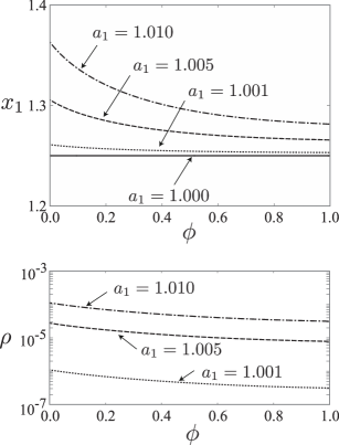
A The Allen–Arkolakis model (unique equilibrium)

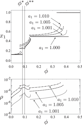
B The Krugman model

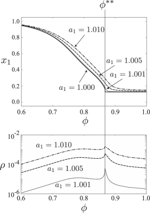
C The Allen–Arkolakis model

Figure F.1: Population share of the advantageous region $1$ and covariance $\rho$

In Figure 1B, the definition of $\rho$ is modified for spatial patterns with unpopulated regions. For the range $\phi\in(\phi^{*},\phi^{**})$, $\rho$ is evaluated with respect to the four-centric pattern $(2\bar{x},0,2\bar{x},0,2\bar{x},0,2\bar{x},0)$:

$$\rho\equiv\sum_{i\in\mathcal{I}(\bm{x})}(x_{i}-2\bar{x})(a_{i}-\bar{a}(\bm{x})),$$ (F.1)

where $\mathcal{I}(\bm{x})=\{i\in\mathcal{I}\mid x_{i}>0\}$ is the set of populated regions and $\bar{a}(\bm{x})\equiv\frac{1}{|\mathcal{I}(\bm{x})|}\sum_{i\in\mathcal{I}(\bm{x})}a_{i}$. We define $\rho$ for two-centric pattern $(4\bar{x},0,0,0,4\bar{x},0,0,0)$ similarly. For the transitional phase after $\phi^{**}$ we let

$$\rho\equiv\sum_{i\in\mathcal{I}(\bm{x})}(x_{i}-x_{i}^{*})(a_{i}-\bar{a}(\bm{x})),$$ (F.2)

where $x_{i}^{*}$ corresponds to the stable solution for the symmetric case ($a_{1}=1$). We have $\rho^{\prime}(\phi)>0$ for the four- and two-centric patterns. This is natural because these patterns may be regarded as the uniform distribution on the four- and two-region cases, respectively.

For Figure 1C, we employ (F.2) as the definition of $\rho$ for the case $\phi\in(0,\phi^{**})$, i.e., we consider the deviation from the baseline equilibrium ($a_{1}=1$). We observe that $\rho^{\prime}(\phi)<0$ does not necessarily hold true for $\phi\in(0,\phi^{**})$. For instance, $\rho^{\prime}(\phi)>0$ when $\phi$ is small. Nonetheless, when the hypothesis of Proposition 2 holds ($\bar{\bm{x}}$ is stable in the baseline case), $\rho$ decreases in $\phi$.

References

- Ahlfeldt et al. (2022) Ahlfeldt, Gabriel M., Thilo Albers, and Kristian Behrens (2022): “A granular spatial model,” CEPR Discussion paper No. 17126.
- Ahlfeldt et al. (2015) Ahlfeldt, Gabriel M., Stephen J. Redding, Daniel M. Sturm, and Nikolaus Wolf (2015): “The economics of density: Evidence from the Berlin Wall,” Econometrica, 83 (6), 2127–2189.
- Akamatsu et al. (2016) Akamatsu, Takashi, Tomoya Mori, and Yuki Takayama (2016): “Agglomerations in a Multi-region Economy: Polycentric versus monocentric patterns,” Discussion papers, Research Institute of Economy, Trade and Industry (RIETI).
- Akamatsu et al. (2012) Akamatsu, Takashi, Yuki Takayama, and Kiyohiro Ikeda (2012): “Spatial discounting, Fourier, and racetrack economy: A recipe for the analysis of spatial agglomeration models,” Journal of Economic Dynamics and Control, 99 (11), 32–52.
- Allen and Arkolakis (2014) Allen, Treb and Costas Arkolakis (2014): “Trade and the topography of the spatial economy,” The Quarterly Journal of Economics, 129 (3), 1085–1140.
- Allen et al. (2019) Allen, Treb, Costas Arkolakis, and Yuta Takahashi (2019): “Universal gravity,” Journal of Political Economy, Forthcoming.
- Anderson and de Palma (2000) Anderson, Simon P. and André de Palma (2000): “From local to global competition,” European Economic Review, 44 (3), 423–448.
- Arkolakis et al. (2012) Arkolakis, Costas, Arnaud Costinot, and Andrés Rodríguez-Clare (2012): “New trade models, same old gains?” American Economic Review, 102 (1), 94–130.
- Bairoch (1988) Bairoch, Paul (1988): Cities and Economic Development: From the Dawn of History to the Present, Chicago: The University of Chicago Press.
- Baldwin et al. (2003) Baldwin, Richard E., Rikard Forslid, Philippe Martin, Gianmarco I. P. Ottaviano, and Frederic Robert-Nicoud (2003): Economic Geography and Public Policy, Princeton University Press.
- Beckmann (1976) Beckmann, Martin J. (1976): “Spatial equilibrium in the dispersed city,” in Mathematical Land Use Theory, ed. by Yorgos Papageorgiou, Lexington Book, 117–125.
- Behrens et al. (2014) Behrens, Kristian, Gilles Duranton, and Frédéric Robert-Nicoud (2014): “Productive cities: Sorting, selection, and agglomeration,” Journal of Political Economy, 122 (3), 507–553.
- Behrens et al. (2017) Behrens, Kristian, Giordano Mion, Yasusada Murata, and Jens Südekum (2017): “Spatial frictions,” Journal of Urban Economics, 97, 40–70.
- Berliant and Mori (2017) Berliant, Marcus and Tomoya Mori (2017): “Beyond urban form: How Masahisa Fujita shapes us,” International Journal of Economic Theory, 13, 5–28.
- Brown and von Neumann (1950) Brown, George W. and John von Neumann (1950): “Solutions of games by differential equations,” in Contributions to the Theory of Games I, ed. by Harold W. Kuhn and Albert W. Tucker, Princeton University Press, 73–80.
- Caliendo et al. (2019) Caliendo, Lorenzo, Maximiliano Dvorkin, and Fernando Parro (2019): “Trade and labor market dynamics: General equilibrium analysis of the China trade shock,” Econometrica, 87 (3), 741–835.
- Davis and Dingel (2020) Davis, Donald R. and Jonathan I. Dingel (2020): “The Comparative Advantage of Cities,” Journal of International Economics, 123, 1032–91.
- Diamond (2016) Diamond, Rebecca (2016): “The determinants and welfare implications of US workers’ diverging location choices by skill: 1980-2000,” American Economic Review, 106 (3), 479–524.
- Dingel et al. (2019) Dingel, Jonathan I., Kyle C. Meng, and Solomon M. Hsiang (2019): “Spatial correlation, trade, and inequality: Evidence from the global climate,” Unpublished manuscript.
- Dupuis and Nagurney (1993) Dupuis, Paul and Anna Nagurney (1993): “Dynamical systems and variational inequalities,” Annals of Operations Research, 44 (1), 7–42.
- Duranton and Puga (2004) Duranton, Gilles and Diego Puga (2004): “Micro-foundations of urban agglomeration economies,” in Handbook of Regional and Urban Economics, ed. by J. Vernon Henderson and Jacques-François Thisse, North-Holland, vol. 4, 2063–2117.
- Duranton and Puga (2019) ——— (2019): “Urban growth and its aggregate implications,” CEPR Discussion Paper No. 1421.
- Forslid and Ottaviano (2003) Forslid, Rikard and Gianmarco I. P. Ottaviano (2003): “An analytically solvable core-periphery model,” Journal of Economic Geography, 33 (3), 229–240.
- Fujita et al. (1999a) Fujita, Masahisa, Paul R. Krugman, and Tomoya Mori (1999a): “On the evolution of hierarchical urban systems,” European Economic Review, 43 (2), 209–251.
- Fujita et al. (1999b) Fujita, Masahisa, Paul R. Krugman, and Anthony Venables (1999b): The Spatial Economy: Cities, Regions, and International Trade, Princeton University Press.
- Fujita and Ogawa (1982) Fujita, Masahisa and Hideaki Ogawa (1982): “Multiple equilibria and structural transformation of non-monocentric urban configurations,” Regional Science and Urban Economics, 12, 161–196.
- Fujita and Thisse (2013) Fujita, Masahisa and Jacques-François Thisse (2013): Economics of Agglomeration: Cities, Industrial Location, and Regional Growth (Second Edition), Cambridge University Press.
- Gaubert (2018) Gaubert, Cecile (2018): “Firm sorting and agglomeration,” American Economic Review, 108 (11), 3117–3153.
- Greenstone et al. (2010) Greenstone, Michael, Richard Hornbeck, and Enrico Moretti (2010): “Identifying agglomeration spillovers: Evidence from winners and losers of large plant openings,” Journal of Political Economy, 118 (3), 536–598.
- Harris and Wilson (1978) Harris, Britton and Alan G. Wilson (1978): “Equilibrium values and dynamics of attractiveness terms in production-constrained spatial-interaction models,” Environment and Planning A, 10 (4), 371–388.
- Heblich et al. (2020) Heblich, Stephan, Stephen J Redding, and Daniel M Sturm (2020): “The making of the modern metropolis: evidence from London,” The Quarterly Journal of Economics, 135 (4), 2059–2133.
- Helpman (1998) Helpman, Elhanan (1998): “The size of regions,” in Topics in Public Economics: Theoretical and Applied Analysis, ed. by David Pines, Efrainm Sadka, and Itzhak Zilcha, Cambridge University Press, 33–54.
- Henderson (1974) Henderson, J. Vernon (1974): “The sizes and types of cities,” American Economic Review, 64 (4), 640–656.
- Hirsch et al. (2012) Hirsch, Morris W., Stephen Smale, and Robert L. Devaney (2012): Differential Equations, Dynamical Systems, and an Introduction to Chaos, Academic Press.
- Horn and Johnson (2012) Horn, Roger A. and Charles R. Johnson (2012): Matrix Analysis (Second Edition), Cambridge University Press.
- Hsu (2012) Hsu, Wen-Tai (2012): “Central place theory and city size distribution,” The Economic Journal, 122, 903–932.
- Ikeda et al. (2012) Ikeda, Kiyohiro, Takashi Akamatsu, and Tatsuhito Kono (2012): “Spatial period-doubling agglomeration of a core–periphery model with a system of cities,” Journal of Economic Dynamics and Control, 36 (5), 754–778.
- Krugman (1991) Krugman, Paul R. (1991): “Increasing returns and economic geography,” Journal of Political Economy, 99 (3), 483–499.
- Krugman (1993) ——— (1993): “On the number and location of cities,” European Economic Review, 37 (2), 293–298.
- Kuznetsov (2004) Kuznetsov, Yuri A. (2004): Elements of Applied Bifurcation Theory (3rd Eds.), Springer-Verlag.
- Lucas and Rossi-Hansberg (2002) Lucas, Robert E. and Esteban Rossi-Hansberg (2002): “On the internal structure of cities,” Econometrica, 70 (4), 1445–1476.
- Matsuyama (2017) Matsuyama, Kiminori (2017): “Geographical advantage: Home market effect in a multi-region world,” Research in Economics, 71, 740–758.
- Mertikopoulos and Sandholm (2018) Mertikopoulos, Panayotis and William H. Sandholm (2018): “Riemannian game dynamics,” Journal of Economic Theory, 177, 315–364.
- Mori et al. (2022) Mori, Tomoya, Takashi Akamatsu, Yuki Takayama, and Minoru Osawa (2022): “Origin of power laws and their spatial fractal structure for city-size distributions,” ArXiv:2207.05346.
- Mori et al. (2020) Mori, Tomoya, Tony E Smith, and Wen-Tai Hsu (2020): “Common power laws for cities and spatial fractal structures,” Proceedings of the National Academy of Sciences, 117 (12), 6469–6475.
- Mumford (1961) Mumford, Lewis (1961): The City in History: Its Origins, Its Transformations, and Its Prospects, New York: A Harvest Book.
- Murata and Thisse (2005) Murata, Yasusada and Jacques-Frano̧is Thisse (2005): “A simple model of economic geography à la Helpman–Tabucbi,” Journal of Urban Economics, 58 (1), 137–155.
- Nash (1951) Nash, John (1951): “Non-cooperative games,” Annals of Mathematics, 54 (2), 286–295.
- Osawa and Akamatsu (2020) Osawa, Minoru and Takashi Akamatsu (2020): “Equilibrium refinement for a model of non-monocentric internal structures of cities: A potential game approach,” Journal of Economic Theory, 187, 105025.
- Osawa et al. (2017) Osawa, Minoru, Takashi Akamatsu, and Yuki Takayama (2017): “Harris and Wilson (1978) model revisited: The spatial period-doubling cascade in an urban retail model,” Journal of Regional Science, 57 (3), 442–466.
- Papageorgiou and Smith (1983) Papageorgiou, Yorgos Y. and Terrence R. Smith (1983): “Agglomeration as local instability of spatially uniform steady-states,” Econometrica, 1109–1119.
- Pflüger (2004) Pflüger, Michael (2004): “A simple, analytically solvable, Chamberlinian agglomeration model,” Regional Science and Urban Economics, 34 (5), 565–573.
- Pflüger and Südekum (2008) Pflüger, Michael and Jens Südekum (2008): “Integration, agglomeration and welfare,” Journal of Urban Economics, 63 (2), 544–566.
- Pflüger and Tabuchi (2010) Pflüger, Michael and Takatoshi Tabuchi (2010): “The size of regions with land use for production,” Regional Science and Urban Economics, 40 (6), 481–489.
- Puga (1999) Puga, Diego (1999): “The rise and fall of regional inequalities,” European Economic Review, 43 (2), 303–334.
- Redding and Rossi-Hansberg (2017) Redding, Stephen J. and Esteban Rossi-Hansberg (2017): “Quantitative spatial economics,” Annual Review of Economics, 9, 21–58.
- Redding and Sturm (2008) Redding, Stephen J. and Daniel Sturm (2008): “The cost of remoteness: Evidence from German division and reunification,” American Economic Review, 98 (5), 1766–1797.
- Sandholm (2010) Sandholm, William H. (2010): Population Games and Evolutionary Dynamics, MIT Press.
- Smith (1984) Smith, Michael J. (1984): “The stability of a dynamic model of traffic assignment: An application of a method of Lyapunov,” Transportation Science, 18 (3), 245–252.
- Tabuchi (1998) Tabuchi, Takatoshi (1998): “Urban agglomeration and dispersion: A synthesis of Alonso and Krugman,” Journal of Urban Economics, 44 (3), 333–351.
- Tabuchi and Thisse (2011) Tabuchi, Takatoshi and Jacques-François Thisse (2011): “A new economic geography model of central places,” Journal of Urban Economics, 69 (2), 240–252.
- Takayama and Akamatsu (2011) Takayama, Yuki and Takashi Akamatsu (2011): “Emergence of polycentric urban configurations from combination of communication externality and spatial competition,” Journal of JSCE Series D3: Infrastructure Planning and Management, 67 (1), 001–020.
- Takayama et al. (2020) Takayama, Yuki, Kiyohiro Ikeda, and Jacques-François Thisse (2020): “Stability and sustainability of urban systems under commuting and transportation costs,” Regional Science and Urban Economics, 84, 103553.
- Taylor and Jonker (1978) Taylor, Peter D. and Leo B. Jonker (1978): “Evolutionarily stable strategies and game dynamics,” Mathematical Biosciences, 40, 145–156.
- United Nations (2018) United Nations (2018): “World Urbanization Prospects 2018,” .
Online Appendix
for “Multimodal Agglomeration in Economic Geography”