Ab initio nuclear thermodynamics

Abstract

We propose a new Monte Carlo method called the pinhole trace algorithm for ab initio calculations of the thermodynamics of nuclear systems. For typical simulations of interest, the computational speedup relative to conventional grand-canonical ensemble calculations can be as large as a factor of one thousand. Using a leading-order effective interaction that reproduces the properties of many atomic nuclei and neutron matter to a few percent accuracy, we determine the location of the critical point and the liquid-vapor coexistence line for symmetric nuclear matter with equal numbers of protons and neutrons. We also present the first ab initio study of the density and temperature dependence of nuclear clustering.

In recent years much progress has been made in ab initio or fully microscopic calculations of the structure of atomic nuclei Stroberg:2016ung ; Piarulli:2017dwd ; Lonardoni:2017hgs ; Gysbers:2019uyb ; Smirnova:2019yiq ; Contessi2017 . These first principles calculations are based on chiral effective field theory, whereby nuclear interactions are included term by term in order of importance Epelbaum:2008ga . Unfortunately, most ab initio methods rely on computational strategies that are not designed for calculations at nonzero temperature. One exception is many-body perturbation theory where diagrammatic expansions are used to calculate bulk thermodynamic properties Baldo:1999cvh ; Holt:2013fwa . Another exception is the method of self-consistent Green’s functions, which provides non-perturbative solutions of the finite temperature system  Soma:2009pf ; Carbone:2018kji ; Carbone:2019pkr ; Carbone:2020 . As with most first principles methods, however, these approaches have difficulties describing cluster correlations, which is an important feature of nuclear multifragmentation and the phase diagram of nuclear matter.

Yet another exception, which we focus on here, is the method of lattice effective field theory. Lattice effective field theory has the advantage that non-perturbative effects such as clustering are reproduced automatically when using Monte Carlo simulations. Early efforts to describe nuclear thermodynamics using lattice simulations exist in the literature Muller:1999cp ; Lee:2004si , but there has been little progress since then. The difficulties stem from the computational cost of performing grand-canonical calculations of nucleons in large spatial volumes. One can reduce the effort by working in a restricted single-particle space Alhassid:2014fca ; Gilbreth:2019gkb . Fully unbiased calculations, however, require a great amount of effort as they use matrices of size $4V\times 4V$, where $V$ is the spatial lattice volume. In this Letter, we report a new paradigm for calculating ab initio nuclear thermodynamics, which we call the pinhole trace algorithm. In this algorithm, the matrices are much smaller, namely of size $A\times A$, where $A$ is the number of nucleons. The resulting computational acceleration can be as large as a factor of one thousand.

The ab initio calculations presented here use the pinhole trace algorithm to implement nuclear lattice effective field theory (NLEFT) Lee2009 ; Lahde2019 at finite temperature. At fixed nucleon number $A$, and temperature $T$, the expectation value of any observable $\mathcal{O}$ is

$$\langle\mathcal{O}\rangle_{\beta}=\frac{Z_{\mathcal{O}}(\beta)}{Z(\beta)}=\frac{{\rm Tr}_{A}(e^{-\beta H}\mathcal{O})}{{\rm Tr}_{A}(e^{-\beta H})},$$ (1)

where $Z(\beta)$ is the canonical partition function, $\beta=T^{-1}$ is the inverse temperature, $H$ is the Hamiltonian, and ${\rm Tr}_{A}$ is the trace over the $A$-nucleon states. Throughout, we use units where $\hbar=c=k_{B}=1$.

The canonical partition function $Z(\beta)$ can be written explicitly in the single particle basis as

$$Z(\beta) = \sum_{c_{1},\cdots,c_{A}}\langle c_{1},\cdots,c_{A}|\exp(-\beta H)|c_{1},\cdots,c_{A}\rangle,$$ (2)

where the basis states are Slater determinants composed of point particles, $c_{i}=({\bm{n}_{i},\sigma_{i},\tau_{i}})$ are the quantum numbers of the $i$-th particle, with $\bm{n_{i}}$ an integer triplet specifying the lattice coordinate, $\sigma_{i}$ is the spin and $\tau_{i}$ is the isospin. On the lattice, the components of $\bm{n_{i}}$ take integer values from 0 to $L-1$, where $L$ is the box length in units of the lattice spacing. The neutron number $N$ and proton number $Z$ are separately conserved, and the summation in Eq. (2) is limited to the subspace with the specified values for $N$ and $Z$.

In the Supplemental Materials we present the full details of the lattice calculations. But in order to explain the basic design of our computational approach, we illustrate here a simplified calculation where the Hamiltonian has a two-body contact interaction

$$H=H_{\rm free}+\frac{1}{2}C\sum_{\bm{n}}:\rho^{2}({\bm{n}}):,$$ (3)

where $H_{\rm free}$ is the free nucleon Hamiltonian with nucleon mass $m=938.9$ MeV, $\rho({\bm{n}})=\sum_{\sigma,\tau}\hat{a}^{\dagger}_{{\bm{n}},\sigma,\tau}\hat{a}_{{\bm{n}},\sigma,\tau}$ is the density operator. The $::$ symbols indicate normal ordering where the annihilation operators are on the right and creation operators are on the left. We assume an attractive interaction with $C<0$.

The imaginary time direction, whose length is set by the inverse temperature $\beta$, is divided into $L_{t}$ slices with time lattice spacing $a_{t}$ such that $\beta=L_{t}a_{t}$. For each time slice the two-body interaction is decomposed using an auxiliary-field transformation such that at each lattice site we have

$$\exp\left(-\frac{a_{t}C}{2}\rho^{2}\right)=\sqrt{\frac{1}{2\pi}}\int ds\exp\left(-\frac{s^{2}}{2}+\sqrt{-a_{t}C}s\rho\right),$$ (4)

where $s$ is the auxiliary field.

Putting these pieces together, we obtain the (auxiliary-field) path-integral expression for Eq. (2)

$$Z(\beta) = \sum_{c_{1},\cdots,c_{A}}\int\mathcal{D}s_{1}\cdots\mathcal{D}s_{L_{t}}\langle c_{1},\cdots,c_{A}|\times$$ (6)

$$M(s_{L_{t}})\cdots M(s_{1})|c_{1},\cdots,c_{A}\rangle,$$

where

$$M(s_{n_{t}})=:\exp\left[-a_{t}K+\sqrt{-a_{t}C}\sum_{{\bm{n}}}s_{n_{t}}({\bm{n}})\rho({\bm{n}})\right]:$$ (7)

is the normal-ordered transfer matrix for time step $n_{t}$, and $s_{n_{t}}$ is our shorthand for all auxiliary fields at that time step Lee2009 ; Lahde2019 . $K=-\nabla^{2}/2M$ is the kinetic energy operator, which is discretized using finite difference formulae Lee2009 . For a given configuration $s_{n_{t}}$, the transfer matrix $M(s_{n_{t}})$ consists of a string of one-body operators which are directly applied to each single-particle wave function in the Slater determinant. For notational convenience, we will use the abbreviations $\vec{c}=\{c_{1},\cdots,c_{A}\}$ and $\vec{s}=\{s_{1},\cdots,s_{L_{t}}\}$.

The pinhole trace algorithm (PTA) was inspired by the pinhole algorithm used to sample the spatial positions and spin/isospin of the nucleons Elhatisari2017 . However, the purpose, implementation, and underlying physics of the PTA for nuclear thermodynamics are vastly different from the original pinhole algorithm used for density distributions. In the PTA we evaluate Eq. (6) using Monte Carlo methods, i.e. importance sampling is used to generate an ensemble $\Omega$ of $\{\vec{s},\vec{c}\}$ of configurations according to the relative probability distribution

$$P(\vec{s},\vec{c})=\left|\braket{\vec{c}}{M(s_{L_{t}})\cdots M(s_{1})}{\vec{c}}\right|.$$ (8)

The expectation value of any operator $\hat{O}$ can be expressed as

$$\langle\hat{O}\rangle=\langle\mathcal{M}_{O}(\vec{s},\vec{c})\rangle_{\Omega}/\langle\mathcal{M}_{1}(\vec{s},\vec{c})\rangle_{\Omega},$$ (9)

where

$$\mathcal{M}_{O}(\vec{s},\vec{c}) = \langle\vec{c}|M(s_{L_{t}})\cdots M(s_{L_{t}/2+1})\hat{O}\times$$ (11)

$$M(s_{L_{t}/2})\cdots M(s_{1})|\vec{c}\rangle/P(\vec{s},\vec{c}).$$

To generate the ensemble $\Omega$ we use the Metropolis algorithm to update $\vec{s}$ and $\vec{c}$ alternately. We first fix the nucleon configuration $\vec{c}$ and update the auxiliary fields $\vec{s}$. Starting from the rightmost time slice $s_{1}$, we update $s_{1},\cdots,s_{L_{t}}$ successively, as detailed in Supplemental Materials.

After updating $\vec{s}$, we then update the nucleon configuration $\vec{c}$. To that end, we randomly choose a nucleon $i$ and move it to one of its neighboring sites

$$c_{i}=\{\bm{n}_{i},\sigma_{i},\tau_{i}\}\rightarrow c^{\prime}_{i}=\{\bm{n}^{\prime}_{i},\sigma_{i},\tau_{i}\},$$ (12)

or flip its spin,

$$c_{i}=\{\bm{n}_{i},\sigma_{i},\tau_{i}\}\rightarrow c^{\prime}_{i}=\{\bm{n}_{i},-\sigma_{i},\tau_{i}\}.$$ (13)

The corresponding new nucleon configuration $\vec{c}\,^{\prime}$ is accepted if

$$P(\vec{s},\vec{c}\,^{\prime})/P(\vec{s},\vec{c})>r^{\prime}$$ (14)

with $0\leq r^{\prime}<1$ a random number. Because in the $\vec{c}$ update only one nucleon is moved or spin flipped at a time, the successive configurations are correlated. Only when all nucleons have been updated do we obtain statistically independent configurations. For calculations described here, we found that about 16 $\vec{c}$ updates for every $\vec{s}$ update produced the optimal sampling efficiency.

At low temperatures the signal in Eq. (2) may be overwhelmed by stochastic noise due to the notorious sign problem, i.e. to the almost complete cancellation between positive and negative amplitudes. In auxiliary-field simulations with attractive pairing interactions, the sign problem is held in check by pairing symmetries. For the case of spin pairing, this means that for any nucleon with quantum numbers $({\bm{n}},\sigma,\tau)$, we can find another nucleon with $({\bm{n}},-\sigma,\tau)$. As the transfer matrix in Eq. (7) is spin-independent, the pairing symmetry is preserved irrespective of the auxiliary fields. A similar pairing symmetry also holds for isospin pairing, with $\tau$ and $-\tau$. These pairing symmetries produce single-nucleon amplitude matrices with eigenvalues that come in complex conjugate pairs, such that the corresponding matrix determinants remain positive.

In the PTA, the nucleon positions and indices are allowed to explore unpaired configurations and could spoil the protection from sign oscillations provided by pairing symmetries. Indeed, this possibility is one reason why the method had not been considered earlier, and why grand-canonical calculations have instead been used for the thermodynamics of nuclear systems as well as ultracold atoms Drut2006 ; Drut2008 . Fortunately, we find that this issue is not realized here. For all temperatures considered in this Letter, we find that the sign problem is rather mild, as the positive sign configurations have stronger amplitudes due to the attractive pairing interactions. However, the sign problem will eventually reemerge for temperatures very low compared to the Fermi energy. For interactions without pairing symmetries, the sign problem will be far more severe and appear even in auxiliary-field Monte Carlo calculations without pinholes.

For the values of $A$, $V$, and $L_{t}$ of interest in this work, the computational scaling of the PTA is $A^{2}VL_{t}$, while that for the grand-canonical algorithm described in Ref. Blankenbecler:1981jt is $AV^{2}L_{t}$. Details of the computational scaling analysis can be found in the Supplemental Materials. The cost savings of the PTA is a factor of $V/A$, and the speed up factor associated with the PTA will be as large as one thousand, depending on the lattice spacing and particle density.

Next we discuss the measurement of the observables. While the energies and density correlation functions can be directly measured by inserting the corresponding operators in the middle time step as in Eq. (9), we still need to design efficient algorithms for computing intensive variables, e.g., chemical potential $\mu$ or pressure $p$. This contrasts with grand-canonical ensemble calculations where the chemical potential is given as an external constraint.

In classical thermodynamics simulations, the Widom insertion method (WIM) Widom1963 is used to determine the statistical mechanical properties Binder1997 ; Dullens2005 . In the WIM we freeze the motion of the molecules and insert a test particle to the system and measure the free-energy difference, from which the chemical potential can be determined. The advantage of the WIM is that we do not need the total free energy, which would require an evaluation of the partition function. In the PTA we encounter a similar problem. The absolute free energy can only be inferred with an integration of the energy from absolute zero, which induces large uncertainties. To solve this problem, we adapt the WIM to the quantum lattice simulations, with the test particles substituted by fermionic particles or holes in the system.

For every configuration $\vec{c}$ generated in the PTA, we calculate the expectation values associated with adding one nucleon or removing on nucleon. We define

$$\mathcal{B}_{1} = \sum_{c^{\prime}}\braket{\vec{c}\cup c^{\prime}}{M(s_{n_{t}})\cdots M(s_{1})}{\vec{c}\cup c^{\prime}}/P(\vec{s},\vec{c}),$$

$$\mathcal{B}_{-1} = \sum_{i}\braket{\vec{c}\setminus c_{i}}{M(s_{n_{t}})\cdots M(s_{1})}{\vec{c}\setminus c_{i}}/P(\vec{s},\vec{c}),$$ (15)

where the summation over $c^{\prime}$ runs over all single particle quantum numbers and the summation over $i$ runs over all existing particles. $P(\vec{s},\vec{c})$ is the probability given in Eq. (8). The extra free energy of inserting or removing one particle is given by

$$F(A\pm 1)-F(A)=-T\ln\left[\frac{\langle\mathcal{B}_{\pm 1}\rangle_{\Omega}}{(A\pm 1)!}\right].$$ (16)

Using the symmetric difference, we have

$$\mu=[F(A+1)-F(A-1)]/2=\frac{T}{2}\ln\left[A(A+1)\frac{\langle\mathcal{B}_{-1}\rangle_{\Omega}}{\langle\mathcal{B}_{1}\rangle_{\Omega}}\right].$$ (17)

In the PTA the summations in Eq. (15) can be calculated using random sampling. For $\mathcal{B}_{1}$ we insert a nucleon with random spin and location and propagate it through all time slices, while for $\mathcal{B}_{-1}$ we simply remove one of the existing nucleon. As only one particle is inserted/removed in each measurement, we find this algorithm very efficient and precise in calculating the chemical potential $\mu$. Subsequently, we determine the pressure $p$ by integrating the Gibbs-Duhem equation, $dp=\rho d\mu$, starting from the vacuum with $p=0,\rho=0$.

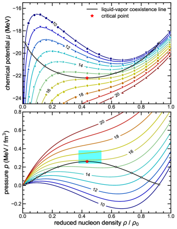
Figure 1: (Upper panel) The $\mu$-$\rho$ isotherms of symmetric nuclear matter computed on the lattice with $L^{3}=6^{3}$. The numbers on the lines are temperatures in MeV, and the temperature difference between adjacent isotherms is 1 MeV. The black line denotes the liquid-vapor coexistence line derived from Maxwell construction, and the red star marks the calculated critical point. (Lower panel) The $p$-$\rho$ isotherms of symmetric nuclear matter are shown for $L^{3}=6^{3}$. The black line denotes the liquid-vapor coexistence line, and the red star marks the calculated critical point. The cyan rectangle marks the empirical critical point extracted from heavy-ion collisions Elliott2013 .

As the long-range Coulomb interaction is ill-defined in the thermodynamic limit without screening, it is standard practice to remove the Coulomb force from nuclear matter calculations. We note that in actual heavy-ion collisions the Coulomb interaction can be important, and so the comparison with Coulomb-removed nuclear matter is not entirely straightforward. We first focus on the nuclear equation of state at nonzero temperatures, which is important for describing the evolution and dynamics of core-collapse supernovae Togashi2017 , neutron star cooling Page2004 , neutron star mergers Most:2018eaw and heavy-ion collisions Das:2004az . We then consider nuclear clustering as a function of density and temperature.

In this work we perform simulations on $L^{3}=4^{3},5^{3},6^{3}$ cubic lattice with up to 144 nucleons and a spatial lattice spacing $a=1/150$ MeV${}^{-1}\approx 1.32$ fm, such that the corresponding momentum cutoff is $\Lambda=\pi/a\approx 471$ MeV. The temporal lattice spacing is taken to be $a_{t}=1/2000$ MeV^-1. For these calculations we use the pionless effective field theory Hamiltonian introduced in Ref. Lu:2018bat , consisting of two- and three-body contact interactions which reproduce the binding energy and charge distribution of many light and medium-mass nuclei. While this is a simple leading order theory and the results are only a first step towards higher-order calculations in chiral effective field theory, our simplified calculation has the important dual purpose of making our discussion of the PTA accessible to a broader audience for potential applications to the thermodynamics of condensed matter systems and ultracold atoms.

We impose twisted boundary conditions along the coordinate directions, which means that each nucleon momentum component $p_{i}$ must equal $\theta_{i}/L+2\pi n_{i}/L$ for our chosen twist angle $\theta_{i}$ and some integer $n_{i}$. As detailed in Supplemental Materials, we average each observable over all possible twist angles by Monte Carlo sampling. As others have found Lin2001 ; Hagen:2013yba ; Schuetrumpf:2016uuk , twist averaging significantly accelerates the convergence to the thermodynamic limit.

In Fig. 1 we present the calculated chemical potential and pressure isotherms for $L^{3}=6^{3}$. Each point represents a separate simulation. The temperature $T$ covers the range from 10 MeV to 20 MeV and densities from 0.0080 fm^-3 to 0.20 fm^-3. The statistical errors are very small, less than 0.02 MeV for $\mu$ and less than 0.002 MeV/fm³ for $p$. These are too small to be clearly visible in Fig. 1 and are not shown. The liquid-vapor coexistence line is determined through the Maxwell construction of each isotherm and depicted as a solid black line in Fig. 1. The liquid-vapor critical point is then located by solving the equations $d\mu/d\rho=d^{2}\mu/d\rho^{2}=0$. The same process applied to the data for $L=4^{3}$ and $L=5^{3}$ in order to estimate the error associated with extrapolation to the thermodynamic limit.

In Table 1 we present the calculated critical temperature $T_{c}$, density $\rho_{c}$ and critical pressure $P_{c}$. The first error bar represents the combined uncertainty from statistics and extrapolation to the thermodynamic limit. The second error bar is the estimated systematic uncertainty associated with the contribution of omitted higher-order interactions. For completeness we also present the saturation density $\rho_{\rm sat}$ at $T=0$ MeV and the saturation energy per nucleon $E_{\rm sat}/A$. We compare our results with the perturbative calculations using N³LO chiral interactions Wellenhofer2014 with two different momentum cutoffs. There appears to be a significant amount of dependence on the momentum cutoff, and the difference gives a rough estimate of the corresponding uncertainties. In the last column we present the empirical values deduced from the heavy-ion collision experiments Elliott2013 .

We note that while the empirical $\rho_{\rm sat}$ extracted from heavy-ion collisions is about $25\%$ lower than the standard value of $0.17$ fm^-3 and our lattice $\rho_{\rm sat}$ is about $25\%$ higher than $0.17$ fm^-3, the ratios for $\rho_{c}/\rho_{\rm sat}$ for the two cases are in agreement with each other and also in agreement with the two N³LO chiral results. This is consistent with the general expectation that small systematic errors in the density can be reduced by computing ratios of densities.

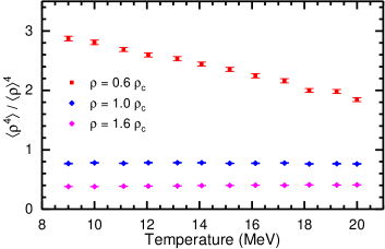
Figure 2: The temperature dependence of the four-body density $\langle:\rho^{4}:\rangle$ scaled by the fourth power of the nucleon density $\langle\rho\rangle$. The results are calculated for symmetric nuclear matter on the lattice with $L^{3}=5^{3}$. The squares, circles, and diamonds represent total nucleon number $A=16,28,40$, respectively. The corresponding nucleon densities are $\rho=0.6\rho_{c},1.0\rho_{c},1.6\rho_{c}$, with $\rho_{c}=0.089$ fm^-3 the calculated critical density.

Table 1: The calculated critical temperature $T_{c}$, pressure $P_{c}$, density $\rho_{c}$, saturation density $\rho_{\rm sat}$ and energy per nucleon $E_{\rm sat}/A$. For comparison we also present the results of perturbative calculations using N³LO chiral potentials, ”n3lo414” and ”n3lo500” correspond to cutoff momentum $\Lambda=414$ and $500$ MeV, respectively Wellenhofer2014 . ”Exp.” denotes the empirical values inferred from the cluster distributions in the multi-fragmentation experiments Elliott2013 .

		This work	n3lo414	n3lo500	Exp.
$T_{c}$(MeV)		$15.80(0.32)(1.60)$	$17.4$	$19.1$	$17.9(4)$
$P_{c}$(MeV/fm3)		$0.260(05)(30)$	$0.33$	$0.42$	$0.31(7)$
$\rho_{c}$(fm-3)		$0.089(04)(18)$	$0.066$	$0.072$	$0.06(1)$
$\rho_{{\rm sat}}$(fm-3)		$0.205(08)(40)$	$0.171$	$0.174$	$0.132$
$E_{{\rm sat}}/A$(MeV)		$-16.9(0.3)(1.7)$	$-15.79$	$-16.51$

Nuclear clustering is another important phenomenon essential to our understanding of the phase diagram of nuclear matter and multifragmentation in heavy-ion collisons Ono:2019 . Here we present the first study of nuclear clustering in a fully ab initio thermodynamics calculation. Nuclear clustering is a manifestation of strong many-body correlations which goes well beyond mean-field theory, and thus is very difficult to reproduce using most ab initio methods. In Fig. 2 we show the expectation values of the four-body density $\langle:\rho^{4}:\rangle$ for different temperatures. To build a dimensionless observable, we scale the results by the nucleon density $\langle\rho\rangle$ to the fourth power. The resulting quantity $\kappa$ is a sensitive indicator of the degree of four-body clustering or alpha clustering. Here we present the results for three different nucleon densities, which correspond to $0.6$, $1.0$ and $1.6$ times the critical density $\rho_{c}$. For sub-critical density $\rho=0.6\rho_{c}$ the system is a plasma of small clusters and we found $\kappa\gg 1$. As the temperature increases the clusters begin to disintegrate and $\kappa$ decreases. For the critical density $\rho=\rho_{c}$ and super-critical density $\rho=1.6\rho_{c}$, we found negligible alpha clustering with $\kappa<1$. Here the thermal motion and small interparticle spacing overwhelm the tendency for clustering in such hot and dense environments. In this regime we find that alpha clustering is a monotonically decreasing function of the nucleon density, but does not depend on the temperature. Since nuclear clustering is very difficult to probe using other ab initio methods, it would be extremely interesting and useful to build upon this first study and investigate the density and temperature dependence of nuclear clustering in more detail with the PTA and high-quality chiral nuclear forces.

Future work will improve upon these calculations by including higher-order interactions in lattice effective field theory. With the pinhole trace algorithm, many exciting applications are possible based on first principles calculations of quantum many-body systems at nonzero temperature. This includes studies of superfluidity in symmetric and asymmetric nuclear matter, neutrino interactions in warm nuclear matter and supernova explosions, the properties of neutron stars and neutron star mergers, the temperature and density dependence of nuclear clusters, and extensions to other quantum many-body systems such as ultracold atoms and molecules.

I Supplemental Materials

I.1 Lattice Hamiltonian

For calculating the nuclear equation of state and four-body clustering we take the leading order pionless effective field theory presented in Ref. Lu:2018bat . In this section we give the details. On a periodic $L^{3}$ cube with lattice coordinates $\bm{n}=(n_{x,}n_{y},n_{z})$, The Hamiltonian is

$$H_{{\rm SU(4)}}=H_{\rm free}+\frac{1}{2!}C_{2}\sum_{\bm{n}}:\tilde{\rho}^{2}(\bm{n}):+\frac{1}{3!}C_{3}\sum_{\bm{n}}:\tilde{\rho}^{3}(\bm{n}):,$$ (S1)

where $H_{\rm free}$ is the free nucleon Hamiltonian with nucleon mass $m=938.9$ MeV and the $::$ symbol indicate normal ordering. The density operator $\tilde{\rho}(\bm{n})$ is defined as

$$\tilde{\rho}(\bm{n})=\sum_{i}\tilde{a}_{i}^{\dagger}(\bm{n})\tilde{a}_{i}(\bm{n})+s_{L}\sum_{|\bm{n}^{\prime}-\bm{n}|=1}\sum_{i}\tilde{a}_{i}^{\dagger}(\bm{n}^{\prime})\tilde{a}_{i}(\bm{n}^{\prime}),$$ (S2)

where $i$ is the joint spin-isospin index and the smeared annihilation and creation operators are defined as

$$\tilde{a}_{i}(\bm{n})=a_{i}(\bm{n})+s_{NL}\sum_{|\bm{n}^{\prime}-\bm{n}|=1}a_{i}(\bm{n}^{\prime}).$$ (S3)

The summation over the spin and isospin implies that the interaction is SU(4) invariant. The parameter $s_{L}$ controls the strength of the local part of the interaction, while $s_{NL}$ controls the strength of the nonlocal part of the interaction. Here we include both kinds of smearing. Both $s_{L}$ and $s_{NL}$ have an impact on the range of the interactions. The parameters $C_{2}$ and $C_{3}$ give the strength of the two-body and three-body interactions, respectively.

In this letter we use a lattice spacing $a=1.32$ fm, which corresponds to a momentum cutoff $\Lambda=\pi/a\approx 471$ MeV. The dynamics with momentum $Q$ much smaller than $\Lambda$ can be well described and residual lattice artifacts are suppressed by powers of $Q/\Lambda$. In this letter we use the parameter set $C_{2}=-3.41\times 10^{-7}$ MeV^-2, $C_{3}=-1.4\times 10^{-14}$ MeV^-5, $s_{L}=0.061$ and $s_{NL}=0.5$. These parameters are adjusted to reproduce the deuteron, triton and the properties of medium mass nuclei.

Nominally we are using a lattice action that can be viewed as a leading order interaction in pionless effective field theory. However it would be misleading to associate the systematic errors of this work with that of other leading order pionless studies such as Ref. Contessi:2017rww . Our collaboration has studied the importance of the range and strength of the local part of the nucleon-nucleon interaction in order to reproduce the bulk properties of nuclear matter Elhatisari:2016owd ; Rokash:2016tqh . The interaction used here utilizes this information in order to reproduce the binding energies and radii of light and medium-mass nuclei and the equation of state of neutron matter with no more than a few percent error. All of the errors associated with the systematic deficiencies of our interactions have been estimated and presented in our results.

we calculate the NN S-wave phase shifts below relative fit errors by comparing results with the and

I.2 Auxiliary field formalism

We simulate the interactions of nucleons on the lattice using projection Monte Carlo with auxiliary fields; see Ref. Lee2009 ; Lahde2019 for an overview of methods used in lattice EFT. We use an auxiliary-field formalism where the interactions among nucleons are replaced by interactions of nucleons with auxiliary fields at every lattice point in space and time. In the auxiliary-field formalism each nucleon evolves as if it is a single particle in a fluctuating background of auxiliary fields. We use a single auxiliary field at LO in the EFT expansion coupled to the total nucleon density. The interactions are reproduced by integrating over the auxiliary field. In our lattice simulations, the spatial lattice spacing is taken to be $a$ = (150 MeV)^-1= 1.32 fm, and the time lattice spacing is $a_{t}$ = (2000 MeV)^-1= 0.0985 fm. For any fixed initial and final state, the amplitude for a given configuration of auxiliary field is proportional to the determinant of an $A\times A$ matrix $M_{ij}$. The entries of $M_{ij}$ are the single nucleon amplitudes for a nucleon starting at state $j$ at $\tau$ = 0 and ending at state $i$ at $\tau$ = $\tau_{f}$.

We use a discrete auxiliary field that can simulate the two-, three- and four-body forces simultaneously without sign oscillations. This follows from an exact operator identity connecting the exponential of the two-particle density $\rho^{2}$ to a sum of the exponentials of the one-particle density $\rho$:

$$:\exp\left(-\frac{1}{2}C\rho^{2}-\frac{1}{6}C_{3}\rho^{3}-\frac{1}{24}C_{4}\rho^{4}\right):=\sum_{k=1}^{N}\omega_{k}:\exp\left(\sqrt{-C}\phi_{k}\rho\right):$$ (S4)

where $C$ is the interaction coefficient, $C_{3}$ and $C_{4}$ are coupling constants for three-body and four-body forces, respectively, $\omega_{k}$’s and $\phi_{k}$’s are real numbers and the :: symbols indicate the normal ordering of operators. In this letter we only consider attractive two-body interactions with $C<0$. In order to avoid the sign problem we further require $\omega_{k}>0$ for all $k$. The implementation of higher-body interactions using auxiliary fields is also discussed in Ref. Korber:2017emn .

To determine the constants $\phi_{k}$’s and $\omega_{k}$’s, we expand Eq. (S4) up to $\mathcal{O}(\rho^{4})$ and compare both sides order by order. In the context of the nuclear EFT, the three- and four-body interactions are usually much weaker than the two-body interaction, and we use the following ansatz with $N=3$,

$$\omega_{1}=\frac{1}{\phi_{1}(\phi_{1}-\phi_{3})},\qquad\omega_{2}=1+\frac{1}{\phi_{1}\phi_{3}},\qquad\omega_{3}=\frac{1}{\phi_{3}(\phi_{3}-\phi_{1})}$$ (S5)

where $\phi_{2}=0$ and $\phi_{1}$ and $\phi_{3}$ are two roots of the quadratic equation,

$$\phi^{2}+\frac{C_{3}}{\sqrt{-C^{3}}}\phi-\frac{C_{3}^{2}}{C^{3}}+(\frac{C_{4}}{C^{2}}-3)=0.$$ (S6)

Using Vieta’s formulas, it is straightforward to verify that Eq. (S5) satisfies Eq. (S4) up to $\mathcal{O}(\rho^{4})$. For a pure two-body interaction $C_{3,4}=0$, the solution is simplified to $\phi_{1}=-\phi_{3}=\sqrt{3}$, $\phi_{2}=0$, $\omega_{1}=\omega_{3}=1/6$, $\omega_{2}=2/3$. The formalism Eq. (S5) is very efficient in simulating the many-body forces non-perturbatively. The corresponding auxiliary field $s(n_{t},\bm{n})$ only assumes three different values $\phi_{1}$, $\phi_{2}$ and $\phi_{3}$ and can be sampled with the shuttle algorithm described below.

I.3 Updating the auxiliary field

We update the auxiliary field $s(n_{t},\bm{n})$ using a shuttle algorithm, in which only one time slice is updated at a time. The shuttle algorithm works as follows. (1) Choose one time slice $n_{t}$, record the corresponding auxiliary field as $s_{{\rm old}}(n_{t},\bm{n}$). (2) Update the corresponding auxiliary fields at each lattice site $\bm{n}$ according to the probablity distribution $P\left[s_{{\rm new}}(n_{t},\bm{n})=\phi_{k}\right]=\omega_{k}$, $k=1,2,3$. Note that $\omega_{1}+\omega_{2}+\omega_{3}=1$. (3) Calculate the determinant of the $A\times A$ correlation matrix $M_{ij}$ using $s_{{\rm old}}(n_{t},\bm{n})$ and $s_{{\rm new}}(n_{t},\bm{n})$, respectively. (4) Generate a random number $r\in[0,1)$ and make the “Metropolis test”: if

$$\left|\frac{\det\left[M_{ij}\left(s_{{\rm new}}(n_{t},\bm{n})\right)\right]}{\det\left[M_{ij}\left(s_{{\rm old}}(n_{t},\bm{n})\right)\right]}\right|>r,$$

accept the new configuration $s_{{\rm new}}(n_{t},\bm{n})$ and update the wave functions accordingly, otherwise keep $s_{{\rm old}}(n_{t},\bm{n})$. (5) Proceed to the neighboring time slice, repeat steps 1)-4), and turn round at the ends of the time series.

The shuttle algorithm is well suited for small $a_{t}$. In this case the number of time slices is large and the impact of a single update is small. As the new configuation is close to the old one, the acceptance rate is high. We compared the results with the HMC algorithm and found that the new algorithm is more efficient. In most cases the number of independent configurations per hour generated by the shuttle algorithm is usually three or four times larger than that generated by the HMC algorithm.

I.4 Computational scaling

We discuss the computational scaling of our pinhole trace algorithm (PTA) simulations and the comparison with grand canonical simulations based on the well-known BSS method first described in Ref. Blankenbecler:1981jt . Both are determinant Monte Carlo algorithms for lattice simulations with auxiliary fields, and so the comparison is relatively straightforward. We consider a system with $A$ nucleons, $V=L^{3}$ spatial lattice points, and $L_{t}$ time steps. We will drop constant factors such as the factor of 4 associated with the number of nucleon degrees of freedom. In the PTA we compute $A$ single nucleon wave functions, where each wave function has $V$ components, and the correlation matrix $M_{ij}$ will be an $A\times A$ matrix. Meanwhile the BSS algorithm requires computing $V$ single nucleon wave functions, where each wave function has $V$ components, and the correlation matrix $M_{ij}$ will be a $V\times V$ matrix.

For both algorithms, we update the auxiliary fields sequentially according to time step. We update all of the auxiliary fields at one time step before moving on to the next time step. We now consider a full sweep that updates all of the auxiliary fields. During this sweep through the auxiliary fields, the cost associated with updating the single nucleon wave functions is $AVL_{t}$ for the PTA and $V^{2}L_{t}$ for the BSS algorithm.

For small $A$ we can update all of the $V$ auxiliary fields for a given time step in parallel. But as $A$ becomes large, we need to perform $A$ separate updates per time step, with $V/A$ auxiliary fields updated at a time. For the PTA, the cost of calculating correlation matrices for the full update over auxiliary fields is $A^{2}VL_{t}$, and the cost of calculating matrix determinants for the full update is $A^{4}L_{t}$. For the BSS algorithm, the cost of calculating correlation matrices for the full update is $VL_{t}$, and the cost of calculating matrix determinants for the full update is $AV^{2}L_{t}$.

The PTA has an additional update associated with the pinholes. The cost of calculating correlation matrices for the full update of all $A$ pinholes is $A^{2}VL_{t}$, and the cost of calculating matrix determinants for the full update is $A^{4}L_{t}$. For the values of $A$, $V$, and $L_{t}$ of interest in this work, the overall computational scaling of the PTA is $A^{2}VL_{t}$, while that for the BSS algorithm is $AV^{2}L_{t}$. We see that the cost savings of the PTA is a factor of $V/A$. We find that the speed up associated with the PTA can be as large as one thousand, depending on the lattice spacing and particle density.

I.5 Autocorrelation and sign problem in the PTA

In this section we test the performance of the PTA in terms of autocorrelation and the sign problem. In Fig. S1 we show the auto-correlation coefficient

$$\rho(n)=\frac{{\rm Cov}[E(n_{0}),E(n_{0}+n)]}{\sqrt{{\rm D}[E(n_{0})]{\rm D}[E(n_{0}+n)]}},$$ (S7)

where $E(n_{0})$ and $E(n_{0}+n)$ are the energies calculated after $n_{0}$ and $n_{0}+n$ update cycles, respectively. ${\rm Cov}$ and ${\rm D}$ are covariance and variance, respectively. It is clearly seen that the auto-correlation time increases with the nucleon number, which means that for larger systems more $\vec{c}$ updates will be needed to accelerate the convergence to equilibrium and reduce the uncertainties. Nevertheless, in all calculations considered here, 16 $\vec{c}$ updates for every $\vec{s}$ update appear to achieve optimal efficiency.

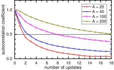
Figure S1: The auto-correlation coefficient of the total energy for the pinhole trace algorithm. $A$ is the number of nucleons, the temperature is $T=10$ MeV and box size is $L=6$. For each update cycle we update the auxiliary field once and pinhole configurations 16 times.

At low temperatures the Monte Carlo simulations face the notorious sign problem, which refers to cancellations between positive and negative amplitudes. The average phase

$$\langle e^{i\theta}\rangle=\langle\mathcal{M}_{1}(\vec{s},\vec{c})\rangle_{\Omega}$$ (S8)

signifies the severity of the sign problem. In practice the calculations become noisy when $\langle e^{i\theta}\rangle$ is less than $0.1$. In Fig. S2 we show the average phase of PTA for temperatures from 1 MeV to 15 MeV in the ¹⁶O nucleus. Here the average phase is a monotonically increasing function of the temperature and asymptotes to 1 at high temperatures. For temperatures as low as 1 MeV, the average phase decreases to $0.3$, which requires a factor of ten times more measurements to achieve the same prescribed precision. Nevertheless, for all temperatures above 1 MeV, we find that the sign problem is rather mild.

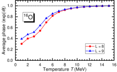
Figure S2: The average phase $\langle e^{i\theta}\rangle$ as a function of the temperature $T$ in ¹⁶O. Circles and triangles denote results for $L=8$ and $L=9$ respectively.

Table S1: Average phase $\langle e^{i\theta}\rangle$ in an $L=6$ box. The Hamiltonian is the leading order pionless contact interactions in Ref. Lu:2018bat .

$T$ (MeV)	16O	17O	18O	144Hf
$10.0$	0.94	0.94	0.93	0.60
$5.0$	0.47	0.45	0.43	0.02
$2.0$	0.19	0.07	0.08	0.01

In Table S1 we present the average phase $\langle e^{i\theta}\rangle$ for several nuclei at different temperatures. It is clear that the sign problem deteriorates for lower temperature or higher density. In all temperatures we find the largest phase for ¹⁶O. The effect of broken pair in ¹⁷O and ¹⁸O is significant for $T=2.0$ MeV, but negligible for $T=5.0$ MeV and above. This implies that the sign problem is due to the fermionic nature of the nucleons, which is quenched either by pairing to form bosons or at high temperatures.

I.6 Benchmark of the Widom insertion method

In this section we benchmark the WIM using a free nucleon gas where the chemical potential can be calculated analytically. In Fig. S3 we compare the Monte Carlo results with the exact solutions. In the grand canonical ensemble, the chemical potential $\mu$ can be determined by solving the equation

$$\int_{0}^{\Lambda}\frac{\rho(\epsilon)}{1+e^{-\beta(\epsilon-\mu)}}d\epsilon=A,$$ (S9)

where

$$\rho(\epsilon)=\frac{2}{\pi^{2}}mV\sqrt{2m\epsilon}$$ (S10)

is the level density for free Fermi gas with two species, $m$ is the nucleon mass, and $\Lambda=(\pi/a)^{2}/(2m)$ is the energy cutoff imposed by the lattice at lattice spacing $a$. In Fig. S3 the solid line shows the exact solutions and the circles show lattice results calculated using the QWIM. The temperature is $T=10$ MeV, and the box size is $L=5$. We see that the lattice results agrees well with the analytic solutions for $A\leq 100$. The deviation for small $A$ can be explained by the difference between the canonical ensemble at fixed $A$ and the grand canonical ensemble at fixed $\mu$.

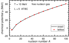
Figure S3: The chemical potential of the free nucleon gas ($N$ = $Z$ = $A/2$) as a function of the nucleon number $A$. The temperature $T=10$ MeV and the box size $L=$5. Average twisted boundary conditions are applied in all directions (as explained below). The circles denote the lattice results using the Widom insertion method. The solid line shows the exact solution in the grand canonical ensemble.

I.7 Backbending of the isotherms

The calculated isotherms we have found follow the pattern expected for a liquid-vapor phase transition in a finite system. Above $T_{c}$ the system is in a supercritical state, while below $T_{c}$ the pure liquid and vapor phases exist in the high- and low-density regime, respectively. For states encompassed by the two arms of the coexistence line, the system is a mixture of the liquid and vapor phases. In the thermodynamic limit, where $N,V\rightarrow\infty$ with $\rho=N/V$ fixed, $\mu$ and $p$ are constants in the coexistence regime along an isotherm. Both $\mu$ and $p$ are uniquely determined by the chemical and mechanical equilibrium conditions, $\mu_{l}=\mu_{v}=\mu_{\rm coex}$ and $p_{l}=p_{v}=p_{\rm coex}$, where the subscripts $l$ and $v$ denote the liquid and vapor phases, respectively. For a finite system the above conditions still hold. However, the surface effects are non-negligible, and $\mu_{\rm coex}$ and $p_{\rm coex}$ can have different values. A well-known example is that the pressure of the vapor in equilibrium with small liquid drops can be larger than its thermodynamic-limit value, with the difference compensated by the contribution of the surface tension. Bearing the importance of the surface contributions in mind, we can easily interpret the ab initio calculations presented in Fig. 1 of the main text.

The most prominent feature of the isotherms in Fig. 1 is the backbending curvature in the coexistence regime below $T_{c}$. Note that the origin of this backbending is completely different from that of similar structures found in the van der Waals model or other mean field calculations. The mean field models describe homogeneous systems and the backbending of the $p$-$\rho$ isotherms result in a negative compressibility. In this regard the assumption of homogeneity conflicts with the condition of mechanical equilibrium. Conversely, in our ab initio calculations we do not rely on the assumption of homogeneity; the results always describe realistic systems. In particular, phase separation occurs spontaneously whenever it is favored by the free energy criterion. In the coexistence regime, the most probable configurations consist of high-density liquid regions and low-density vapor regions, the surface separating these regions gives rise to a positive contribution to the total free energy, which prohibits the formation of small liquid drop in vapor or small bubbles in liquid. The distortions of the isotherms reflect the efforts of the system to overcome such a surface energy barrier.

In Fig. S4 we show schematic plots illustrating the underlying mechanism. Given a fixed volume $V$ and a temperature $T$ below the critical value $T_{c}$, the free energy $F$ is a function of the nucleon number $A$. In the middle panel of Fig. S4 we show the free energy curve across the liquid-vapor coexistence region. We subtract $\mu_{\rm coex}A$ from $F$ to remove most of the $A$-dependence, with $\mu_{\rm coex}$ assuming the value at the thermodynamic limit. For a finite system the surface free energy $F_{\rm surf}$ is approximately proportional to the area of the surface. In the upper panel of Fig. S4 we show the most probable configurations for different densities. At low densities we have a nucleus surrounded by small clusters, while at high densities we see bubbles in a nuclear liquid. At intermediate densities the system contains bulk nuclear matter with appreciable surface areas. The surface area first increases after the formation of a nucleus then decreases when most of the volume is occupied by the liquid phase. Correspondingly $F_{\rm surf}$ has a unique maximum and creates a bump in the free energy curve. In the lower panel of Fig. S4 we show the corresponding chemical potential $\mu=\partial{F}/\partial{A}$. The backbending is a natural result of the surface free energy contributions.

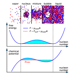
Figure S4: The schematic plots of the vapor-liquid phase transition in a finite nuclear system with fixed volume $V$ and temperature $T<T_{c}$. (Upper panel) The most probable configurations for different nucleon number $A$. Red (blue) points stand for protons (neutrons). The dashed lines signify the surfaces separating the liquid and vapor phases. (Middle panel) The free energy. Solid (dashed) lines denote the results with (without) the surface contributions. (Lower panel) The chemical potential $\mu=\partial{F}/\partial{A}$.

I.8 Finite volume effects

In any first principles calculation of a quantum many-body system, we are necessarily working with finite number of nucleons in a finite volume. The finite volume together with the chosen boundary condition will induce fictitious shell effects. New lattice magic numbers for protons or neutrons emerge where the calculated observables exhibit unphysical kinks. It was observed that 66 particles for one species of spin-1/2 fermions give results close to the thermodynamic limit. This number was extensively used in most of the nuclear matter, neutron matter or cold atom simulations Forbes2011 ; Carlson2011 . However one would ideally like to explore different densities by varying the number of nucleons as well as different the lattice volumes. For this we must reduce as much as possible the problem of ficitious shell effects.

The origin of the finite volume shell effects is the constraint imposed by the boundary conditions on the particle momenta. For a cubic box with periodic boundary conditions (PBC), particles are only allowed to have momenta $\bm{p}=\frac{2\pi}{L}\bm{n}$, which results in a series of magic numbers 2, 14, 38, $\cdots$ for one species of spin-1/2 fermions. One solution is to use twisted boundary conditions (TBC) Byers1961 which attach extra phases to wave functions when particles cross the boundaries. In this case the particle momenta are $\bm{p}=\bm{\theta}+\frac{2\pi}{L}\bm{n}$ for some chosen twist angles $\bm{\theta}$. It has been found that averaging over all possible twist angles provides an efficient way of approaching the infinite volume limit Loh1988 ; Valenti1991 ; Hagen:2013yba ; Schuetrumpf:2016uuk .

The TBC method was first proposed for exactly solvable models Loh1988 ; Valenti1991 ; Gros1992 ; Gammel1993 ; Gros1996 and then found applications in quantum Monte Carlo methods Lin2001 . Many groups have applied TBC to lattice QCD calculations to find infinite volume results otherwise not accessible Bedaque2004 ; Divitiis2004 ; Bedaque2005 ; Sachrajda2004 . Meanwhile, the application of TBC to lattice effective field theory was shown to be successful, though still limited to few-body and exactly solvable systems Korber2016 . In this section we discuss the application of the TBC to lattice Monte Carlo calculations and show how it helps remove finite-volume shell effects in thermodynamics calculations.

We apply the twisted boundary conditions to the single particle wave functions,

$$\psi(x+L,y,z,\sigma,\tau) = \exp(i2\sigma\theta_{x})\psi(x,y,z,\sigma,\tau),$$

$$\psi(x,y+L,z,\sigma,\tau) = \exp(i2\sigma\theta_{y})\psi(x,y,z,\sigma,\tau),$$

$$\psi(x,y,z+L,\sigma,\tau) = \exp(i2\sigma\theta_{z})\psi(x,y,z,\sigma,\tau),$$ (S11)

where $-\pi\leq\theta_{x}$, $\theta_{y}$, $\theta_{z}<\pi$ are the independent twist angles in the three directions. Note that for spin $\sigma=\pm 1/2$ we use the opposite twist angles, which is necessary to preserve time reversal symmetry and avoid sign cancellations. In this paper we employ TBC by averaging over all possible $(\theta_{x},\theta_{y},\theta_{z}),$ which we call average twisted boundary conditions, ATBC. This can be easily implemented in Monte Carlo calculations by allocating to every thread a random phase triplet with elements uniformly distributed in the interval $[-\pi,\pi)$.

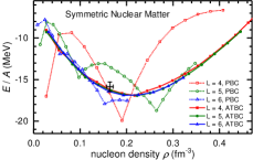
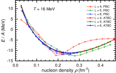
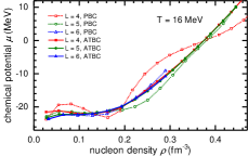
Figure S5: (Upper panel) The binding energy per nucleon calculated with periodic boundary conditions (open symbols) and average twisted boundary conditions (full symbols, as explained below). The temperature is $T=0$ MeV. The squares, circles and triangles show the results calculated with box sizes $L=$ 4, 5 and 6, respectively. The cross with error bars shows the empirical saturation density and binding energy. (Middle panel) The binding energy per nucleon for $T=$ 16 MeV. (Lower panel) The chemical potential at $T=16$ MeV.

In Fig. S5 we compare the binding energies at $T=0$ and $T=16$ MeV and the chemical potential at $T=16$ MeV calculated with different boundary conditions. For the same density, different box sizes correspond to different nucleon numbers. The open symbols denote the results calculated with periodic boundary conditions, the full symbols show the results for the average twisted boundary conditions. Here we see clear shell effects for the PBC calculations. For each box size the energy and chemical potential oscillates with respect to the nucleon number and exhibit extrema at lattice magic numbers $A=$ 4, 28, 76, $\cdots$. The amplitudes of the oscillation are smaller for larger boxes, but for $L=6$ the ficitious shell effects are still apparent. For example, for $T=0$ MeV the energy minimum occurs at $\rho\approx 0.153$ fm^-3, which is a shell effect that corresponds to $A=76$. These results can be misleading if we do not take into account the finite volume corrections.

With ATBC, each of the kinks found above disappear and the results collapse onto universal curves. The chemical potential or the Fermi level, which is very sensitive to the shell structure, can now be precisely calculated and the results for $L=4,5,6$ can be used to estimate the uncertainty in the extrapolation to the thermodynamic limit.

Some remarks must be added for the finite volume effects. Here we distinguish between finite volume effects and finite size effects. The former comes into play together with the boundary conditions and can be removed by using twisted boundary conditions. However, the latter is due to the finite particle number and manifests itself mainly through the surface effects. That is, the finite size effects are maximized for inhomogeneous systems, in particular, the system comprising of two or more phases. The contact surfaces of the different phases give positive contributions to the free energy, which will vanish at the thermodynamic limit. For example, for symmetric nuclear matter with sub-saturation density, the system we described can be viewed as a large volume of liquid containing a number of small bubbles, with bubble density $\rho=1/V$, where $V$ is the volume used in the simulation. For large $V$ at fixed density, the bubbles merge together into large ones and the surface effects will eventually disappear.

The finite size effects scale with the surface-volume ratio, which in turn scales as $O(A^{-1/3})$ with respect to the nucleon number. Thus these effects decay very slowly and cannot be removed with present computational settings. One example of the surface effects are the upbending of the $T=0$ energy curves at low densities in Fig. S5. For infinite nuclear matter, at the sub-saturation densities the density and the binding energy per nucleon will be exactly the value at the saturation point. However, for finite systems the extra surface energy causes the upbending of the energy curve and makes it converging to the binding energy per nucleon of small nucleus in the vacuum, $E/A\approx-8$ MeV.

In Fig. S6 we show the energy per nucleon at $T=0$ calculated with different box sizes. In order to show the finite size effects we have removed the finite volume effects by imposing the average twisted boundary conditions. The calculated energies at sub-saturation energy tend to increase with respect to the box size. However, the convergence is extremely slow. To reduce the finite size effects by one order of magnitude, we have to use $10^{3}$ times more nucleons and $10^{3}$ times larger volume, which is not affordable at present.

We must stress that the existence of the surface effects at phase coexistence is not a deficiency of our method. Instead of studying the infinite homogeneous matter, our method focuses on the real finite systems with phenomena like cluster and phase separation. Consequently, we believe that our formalism, together with the advanced nuclear interactions, will pave the way of fully understanding the nuclear thermodynamic processes.

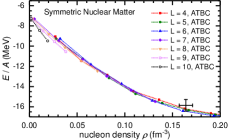
Figure S6: The energy per nucleon at $T=0$ MeV calculated with box sizes from $L=4$ to $L=10$. Average twisted boundary conditions are imposed in all directions. The cross with error bars shows the empirical saturation point.

I.9 Interpolation and error analysis

In extracting the equation of state and critical point, we make an interpolation for the lattice results using the fifth-order virial expansion,

$$\mu(\rho,T)=a_{0}+a_{1}\ln\rho+\sum_{i=1}^{4}a_{i+1}\rho^{i},$$ (S12)

where $a_{i}$ are functions of $T$ and should be fitted for each isotherm separately. Note that this expression is only meant to parametrize the isotherms and the resulting parameters cannot be compared directly with the real virial coeffcients. For non-integer temperatures the chemical potential is obtained by cubic spline interpolation. We the use the interpolated equation of state for differentiation and integration.

The errors in the critical values are estimated by the bootstrap method whereby we resample each lattice result with variance given by the Monte Carlo simulation results several times, and estimate the variance of the critical values by the resulting distribution.

References

- (1) B. N. Lu, N. Li, S. Elhatisari, D. Lee, E. Epelbaum and U.-G. Meißner, Phys. Lett. B 797, 134863 (2019).
- (2) L. Contessi, A. Lovato, F. Pederiva, A. Roggero, J. Kirscher and U. van Kolck, Phys. Lett. B 772, 839-848 (2017).
- (3) S. Elhatisari, N. Li, A. Rokash, J. M. Alarcón, D. Du, N. Klein, B. n. Lu, U. G. Meißner, E. Epelbaum, H. Krebs, T. A. Lähde, D. Lee and G. Rupak, Phys. Rev. Lett. 117, no.13, 132501 (2016).
- (4) A. Rokash, E. Epelbaum, H. Krebs and D. Lee, Phys. Rev. Lett. 118, no.23, 232502 (2017)
- (5) D. Lee, Prog. Part. Nucl. Phys. 63, 117 (2009).
- (6) T. A. Lähde, U.-G. Meißner, “Nuclear Lattice Effective Field Theory: An Introduction”, Lecture Notes in Physics, Volume 957, Springer, (2019).
- (7) C. Körber, E. Berkowitz and T. Luu, EPL 119, no.6, 60006 (2017)
- (8) R. Blankenbecler, D. J. Scalapino and R. L. Sugar, Phys. Rev. D 24, 2278 (1981),
- (9) M. Forbes, S. Gandolfi, and A. Gezerlis, Phys. Rev. Lett. 106, 235303 (2011).
- (10) J. Carlson, Sefano Gandolfi, Kevin E. Schmidt, Shiwei Zhang, Phys. Rev. A 84, 061602R (2011).
- (11) N. Byers and C. N. Yang, Phys. Rev. Lett. 7, 46 (1961).
- (12) E. Y. Loh, Jr. and D. K. Campbell, Synthetic Metals 27, A499 (1988).
- (13) G. Hagen, T. Papenbrock, A. Ekström, K. A. Wendt, G. Baardsen, S. Gandolfi, M. Hjorth-Jensen and C. J. Horowitz, Phys. Rev. C 89, no. 1, 014319 (2014).
- (14) B. Schuetrumpf, W. Nazarewicz and P.-G. Reinhard, Phys. Rev. C 93, no. 5, 054304 (2016).
- (15) R. Valenti, C. Gros, P. J. Hirschfeld and W. Stephan, Phys. Rev. B 44, 13203 (1991).
- (16) C. Gros, Z. Phys. B 86, 359 (1992).
- (17) J. Tinka Gammel, D. K. Campbell, and E. Y. Loh, Jr., Synthetic Metals 55, 4437 (1993).
- (18) C. Gros, Phys. Rev, B 53, 6865 (1996).
- (19) C. Lin, F.-H. Zong, D. M. Ceperley, Phys. Rev. E 64, 016702 (2001).
- (20) Paulo F. Bedaque, Phys. Lett. B 593, 82 (2004).
- (21) G. M. Divitiis, R. Petronzio, N. Tantalo, Phys. Lett. B 595, 408 (2004).
- (22) Paulo F. Bedaque, Jiunn-Wei Chen, Phys. Lett. B 616, 208 (2005).
- (23) C. T. Sachrajda, G. Villadoro, Phys. Lett. B 609, 73 (2005).
- (24) C. Körber, T. Luu, Phys. Rev. C 93, 054002 (2016).