Learning from Noisy Anchors for One-stage Object Detection

Abstract

State-of-the-art object detectors rely on regressing and classifying an extensive list of possible anchors, which are divided into positive and negative samples based on their intersection-over-union (IoU) with corresponding ground-truth objects. Such a harsh split conditioned on IoU results in binary labels that are potentially noisy and challenging for training. In this paper, we propose to mitigate noise incurred by imperfect label assignment such that the contributions of anchors are dynamically determined by a carefully constructed cleanliness score associated with each anchor. Exploring outputs from both regression and classification branches, the cleanliness scores, estimated without incurring any additional computational overhead, are used not only as soft labels to supervise the training of the classification branch but also sample re-weighting factors for improved localization and classification accuracy. We conduct extensive experiments on COCO, and demonstrate, among other things, the proposed approach steadily improves RetinaNet by $\sim$2% with various backbones.

1 Introduction

Object detectors aim to identify rigid bounding boxes that enclose objects of interest in images and have steadily improved over the past few years. Key to the advancement in accuracy is the reduction of object detection to an image classification problem. In particular, a set of candidate boxes, i.e., anchors, of various pre-defined sizes and aspect ratios, are extensively used to be regressed to desired locations and classified into object labels (or background). While training the regression branch is straightforward with ground-truth (GT) coordinates of objects available, optimizing the classification network is challenging: only a small fraction of anchors sufficiently overlap with GT boxes. This limited number of proposals are considered as positive samples, together with a vast number of remaining negative anchors, to learn good classifiers with the help of techniques like focal loss [22] or hard sample mining methods [36, 31, 26] that can mitigate data imbalance problems.

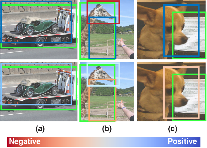
Figure 1: Candidate anchors and their assigned labels (represented by color) in sampled images. Top: classical training methods assign binary labels, i.e., positive (in blue) and negative (in red) to anchors based on IoU between candidates and ground-truth boxes (in green). Bottom: soft labels, represented by the density of colors, assigned to anchors by our approach based on a proposed cleanliness metric for anchors. Best viewed digitally.

Despite the success of such training schemes in various detectors [30, 28, 24, 21, 22], the split of positive and negative anchors relies on a design choice—proposals whose IoUs with GT boxes are higher than a pre-defined foreground threshold are considered as positive samples while those with IoUs lower than a background threshold are treated as negative. Although simple and effective, the use of pre-defined thresholds is simply based on ad-hoc heuristics, and more importantly, the resulting hard division of anchors as either positive or negative is questionable. Unlike standard image classification problems where positive and negative samples are more clearly determined by whether an object occurs, anchors that overlap with GT boxes correspond to patches of objects, covering a fraction of an object’s extent and thus containing only partial information. Therefore, labels assigned to anchors conditioned on their overlap with GT boxes, are ambiguous. For example, the giraffe head in Figure 1 will be considered as a negative sample since the IoU is low, yet it contains meaningful semantic information useful for both localization and classification. In addition, an axis-aligned candidate with satisfactory overlapping with a GT box might contain background clutter and even other objects (see the green car on the truck and the dog in front of the laptop in Figure 1), due to the limitations of representing objects using rectangles. Therefore, labels used to train the classification branch are noisy, and it is challenging to define perfectly clean labels as there is no oracle information to measure the quality of proposals. In addition, noise in labels is further amplified with sampling methods [31, 26] or focal loss [22], since ambiguous and noisy samples tend to produce large losses [2].

In light of this, we explicitly consider label noise for anchors with an aim to reduce its impact during classification and regression. In particular, we associate a cleanliness score with each anchor to adaptively adjust its importance during training. Defining cleanliness is non-trivial, since information on the quality of anchors is limited. However, these scores are expected to be (1) determined automatically rather than based on heuristics; (2) soft and continuous so that anchors are not split into positive and negative set with a hard threshold; (3) can reflect the probability of anchors to be successfully regressed to desired locations and classified into object (or background) labels.

It has been demonstrated that the outputs from networks can indicate the noise level of samples when labels are corrupted and noisy for image classification tasks—the network tends to learn clean samples quickly early on and make confident predictions for them, while recognizing noisy samples slowly yet progressively [13, 15, 29, 34, 18]. In this spirit, we use network outputs as proxies to estimate cleanliness for anchors. We define the cleanliness score of an anchor as a combination of localization accuracies from the regression subnetwork and prediction scores produced by the classification head. Such a definition not only satisfies the aforementioned desiderata but also correlates the classification branch with its regression counterpart. This injects localization information to the classification subnetwork, and thus reduces the discrepancies between training and testing, since proposals are simply ranked based on classification confidence with NMS, unaware of localization accuracy during evaluation.

The cleanliness scores then serve as soft labels to supervise the training of the classification branch. Since they reflect the uncertainty of network predictions and contain richer information than binary labels, this prevents the network from generating over-confident predictions for noisy samples. Furthermore, the cleanliness scores, through a non-linear transformation, are used as sample re-weighting factors to regulate the contributions of different anchors to loss functions for both classification and regression networks. This assists the model to attend to samples with high cleanliness scores, indicating both accurate regression and classification potentials, and to ignore noisy anchors. It worth pointing out the scores based on the outputs of networks are derived without incurring additional computational cost, and can be readily plugged into anchor-based object detectors.

We conduct extensive studies on COCO with state-of-the-art one-stage detectors, and demonstrate that our method improves baselines by $\sim$ 2$\%$ using various backbone networks with minimal surgery to loss functions. In particular, with the common practice [12] of multi-scale training, our approach improves RetinaNet [22] to 41.8% and a 44.1% AP with ResNet-101 [14] and ResNeXt-101-32$\times$8d [39] as backbones, respectively, which are 2.7% and 3.3% higher than the original RetinaNet [22] and better or comparable with state-of-the-art one-stage object detectors. We additionally show the proposed approach can also be applied to two-stage detectors for improved performance.

2 Related Work

Anchor-based object detectors.

Inheriting from the traditional sliding-window paradigms, most modern object detectors perform classification and box regression conditioned on a set of bounding box priors [28, 24, 30, 22, 2, 33, 19]. In particular, one-stage detectors like RetinaNet [22], SSD [24] and YOLOv2 [28] use pre-defined anchors directly, while two-stage detectors like Faster R-CNN [30] use generated region proposals refined from anchors either once or in a cascaded manner. A multitude of detectors have been newly proposed based on these frameworks [32, 37, 25, 2, 44, 7, 6, 46, 4]. However, they rely on pre-defined IoU thresholds to assign binary positive and negative labels to proposals in order to train the classification branch. Instead, we associate each box with a carefully designed cleanliness score as soft labels, dynamically adjusting the contributions of different proposals and hence makes the training noise-tolerant.

Anchor-free object detectors.

There are a few recent studies attempting to address the issues caused by the use of anchors by formulating object detection as a keypoint localization problem. In particular, they aim to localize object keypoints, such as corners [16], centers [40, 8] and representative points covering [35] or circumscribing [42] the spatial extent of objects. The discovered keypoints are either grouped into boxes directly [16, 8] or used as reference points for box regression [35, 42, 40]. They achieve comparable accuracies with anchor-based counterparts, confirming that the conventional classification supervision using anchors is not perfect. However, these keypoint-based methods often require more training time to converge. Instead, we improve anchors with slight modifications to loss functions based on the introduced cleanliness scores. This facilitates efficient training yet competitive performance without additional computational cost.

Sampling/re-weighting in object detection.

The training of object detectors often faces a huge class imbalance due to the large percentage of background candidates. A common technique to address the imbalance is sampling batches with a fixed foreground-to-background ratio [11, 30]. In addition, various hard [31, 26, 5, 24] and soft [22, 17, 3] sampling strategies have been proposed. The core idea of them is to prevent easy samples from overwhelming the loss and then focus the training on hard samples. Despite their effectiveness, these sampling strategies tend to amplify the noise caused by the imperfect split of positive and negative samples, since confusing samples are observed to produce larger losses[13, 1]. We demonstrate that our method is complementary to these sampling methods while alleviates the impact of noise for training.

Learning with noisy labels.

Extensive studies have been conducted on learning from noisy labels, where noise is generally modeled by deep neural networks [15, 13, 34, 18, 29] or graphical models [38, 20], etc. Then, outputs from these models are used to re-weight training samples or infer the correct labels. These approaches focus on the task of image classification where noise is from incorrect annotation or caused by the use of weakly-labeled web images from social media or search engines. In contrast, our focus is on object detection, where label noise results from the imperfect split of positive and negative candidates produced by the solely IoU-based label assignment strategy.

3 Background

We briefly review the standard protocols and design choices for training one-stage detectors and discuss their limitations. State-of-the-art one-stage detectors take as inputs raw images and produce a set of candidate proposals (i.e., anchors), in the form of feature vectors, to predict the labels of potential objects with a classification branch, and regress coordinates of ground-truth bounding boxes through a regression branch. In particular, the regression branch typically uses a smoothed $\ell_{1}$ loss [10] to encourage correct regression of bounding boxes while the classification counterpart incentivizes accurate predictions of object (or background) labels through a binary cross entropy (BCE) loss :

$$\texttt{BCE}\,(p,t)=-t\cdot w_{p}\cdot\texttt{log}(p)-(1-t)\cdot w_{n}\cdot\texttt{log}(1-p),$$ (1)

where $t\in$ {0, 1} denotes the label of a candidate box with background (bg) as 0 and foreground (fg) as 1, and $p\in$ [0, 1] is the predicted classification confidence. $w_{p}$ and $w_{n}$ denote the weighting parameter used in focal loss [22], to down-weight well-classified samples. In contrast to standard image classification tasks where labels are more clearly defined based on the presence of objects, the labels of anchors serving as supervisory signals are artificially defined based on their overlapping with GT-boxes in the following way:

$$t=\begin{cases}1&\text{if }\,\text{IoU}\geq\texttt{fg-threshold}\\ 0&\text{if }\,\text{IoU}<\texttt{bg-threshold}\\ -1&\text{otherwise}.\\ \end{cases}$$ (2)

The fg-threshold is typically set to $0.5$, which is in part motivated by the PASCAL VOC [9] detection benchmark [31] and has been empirically found to be effective for a variety of detectors. Similarly, a box is labeled as background if its IoU with GT is less than the bg-threshold, which is set to $0.4$ in RetinaNet [22].

While offering top-notch performance in most popular detectors, the heuristic approach of identifying positive and negative samples might not be ideal as the thresholds are manually selected and fixed for all objects, regardless of their categories, shapes, sizes, etc. For example, a candidate box with a high IoU for irregular-shaped objects might contain background clutter or even other objects. On the other hand, anchors with smaller IoUs might still contain important clues. For instance, the candidate box containing a giraffe head in Figure 1 would be considered as background, but it contains useful appearance information for recognizing and localizing a giraffe. This hard label assignment leads to noisy samples which are difficult to learn and produce relatively large losses. As a result, noise will be magnified when re-sampling methods like OHEM [31] or focal loss [22] are used to mitigate class imbalance and easy sample dominance problems, since more attention is paid to these hard but probably not meaningful proposals.

4 Our Approach

As discussed above, noise incurred by the imperfect split of positive and negative samples and the limitations of representing objects with rectangles, not only confuses the classification branch to derive good decision boundaries but also misleads re-sampling/weighting methods. Therefore, we propose to reduce the impact of noisy proposals by dynamically adjusting their importance. To accomplish this, we introduce the notion of cleanliness for anchors based on their the likelihood to be successfully classified and regressed. Cleanliness scores are continuous in order to adaptively control the contribution of different proposals.

Recent advances on learning from noisy labels when training networks suggest that the confidence scores of networks indicates the noise level of samples when making predictions, i.e., networks can easily learn easy samples with high confidence while tending to make uncertain predictions for hard and noisy samples. Motivated by this observation, we define the cleanliness scores of anchors using knowledge learned from the classification and localization branches in detectors:

$$c=\begin{cases}\alpha\cdot\texttt{loc\_a}+(1-\alpha)\cdot\texttt{cls\_c}\quad&\text{for}~{}b\in\mathcal{A}_{pos}\\ 0&\text{for}~{}b\in\mathcal{A}_{neg}.\\ \end{cases}$$ (3)

Here, $b$ is a candidate box, loc_a and cls_c denote the localization accuracy and the classification confidence, respectively, and $\alpha$ is a control parameter, balancing the impact of localization and classification. In addition, $\mathcal{A}_{pos}$ and $\mathcal{A}_{neg}$ separately represent positive and negative candidate sets from top-N proposals for each GT-object based on their IoU before box refinement. Note that most candidate boxes only cover background regions due to the dense placement of anchors and should not be labeled and learned as positive samples; consequently, we only assign cleanliness scores to a set of plausible positive candidates, with others labeled as 0. Furthermore, we use direct outputs from the classification network as cls_c and instantiate loc_a as IoU between regressed candidate box and its matched GT-object. Note that although we use network outputs, the approach does not suffer from cold start—initial values of cls_c and output from regression branch are both small, so the derived cleanliness score is an approximation of IoU between anchor and matched GT-object, which does not destablize training during the first few iterations.

Soft labels.

The cleanliness scores are readily used as soft labels to control the contributions of different anchors to the BCE loss in Equation 1 by replacing $t$ with $c$. Since cleanliness scores are dynamically estimated based on the trade-off between loc_a and cls_c, the network can focus on clean samples and not on improperly labeled noisy samples. In addition, these soft and continuous labels allows the network to be more compatible with detection evaluation protocols, where all final predictions are ranked based on their classification scores in NMS, as will be shown in the experiments. The reasons are two-folds: (1) soft labels prevent the model from generating over-confident binarized decisions, producing more meaningful rankings; (2) the localization accuracies are modeled in the soft labels, reducing the misalignment between classification and localization.

Algorithm 1 The algorithm of our approach.

Input: $\mathcal{I}$, $\mathcal{GT}$, $\mathcal{B}$, cls_c, loc_a, $\alpha$, $\gamma$, $N$
$\mathcal{I}$ is the input image,
$\mathcal{GT}$ is the set of ground truth objects within $\mathcal{I}$,
$\mathcal{B}$ is the set of candidates boxes (i.e. anchors),
cls_c is the classification confidence of corresponding ground truth class for candidates,
loc_a is the localization accuracy of candidates,
$\alpha,\gamma$ are the modulating factors, $N$ controls size of positive candidate set.
Output: Losses for classification and box regression $L_{cls},L_{reg}$.

1:$\mathcal{A}_{pos},\mathcal{A}_{neg},S\leftarrow\varnothing$

2:for $gt\in\mathcal{GT}$ do

3:    $indices=argsort($IoU$(\mathcal{B},gt))$ $\triangleright$ Sort in descending order.

4:    $\mathcal{A}_{pos}\leftarrow\mathcal{A}_{pos}\cup\{indices[0:N]:gt\}$

5:end for

6:$\mathcal{A}_{neg}\leftarrow\{(\mathcal{B}-\mathcal{A}_{pos}).indices:0\}$

7:for $b_{i}\in\mathcal{A}_{pos}$ do

8:    $c=\alpha\cdot\texttt{loc\_a}_{i}+(1-\alpha)\cdot\texttt{cls\_c}_{i}$ $\triangleright$ Equation 3

9:    $r=(\alpha\cdot f(\texttt{loc\_a}_{i})+(1-\alpha)\cdot f(\texttt{cls\_c}_{i}))^{\gamma}$ $\triangleright$ Equation 4

10:    $S\leftarrow S\cup\{b_{i}:\{c,r\}\}$

11:end for

12:for $b_{i}\in\mathcal{A}_{neg}$ do $S\leftarrow S\cup\{b_{i}:\{c\leftarrow 0.0,r\leftarrow 1.0\}\}$ end for

13:$L_{cls}=\Sigma_{i}^{S}r_{i}\cdot$ BCE$(p_{i},c_{i})$ $\triangleright$ Equation 5

14:$L_{reg}=\Sigma_{i}^{S}r_{i}\cdot$ $\texttt{smooth}\_\ell_{1}$ $\triangleright$ Equation 6

15:return $L_{cls},L_{reg}$

Sample re-weighting.

One-stage detectors are usually confronted with a severe imbalance of training data with a large amount of negative proposals and only a few positive ones. To mitigate this issue, focal loss [22] decreases the loss of easy samples and focuses more on hard and noisy samples. However, for proposals with label noise, they will be stressed during training even though they could simply be outliers. Therefore, we also propose to re-weight samples based on cleanliness scores defined in Equation 3. While we could to directly use Eqn. 3 for re-weighting, the variations of cleanliness scores among different proposals are not significantly large as loc_a and cls_c are normalized. To encourage a large variance, we pass loc_a and cls_c through a non-linear function $f(x)=\frac{1}{1-x}$. The re-weighting factor $r$ for each box $b\in\mathcal{A}_{pos}$ becomes:

$$r=(\alpha\cdot f(\texttt{loc\_a})+(1-\alpha)\cdot f(\texttt{cls\_c}))^{\gamma},$$ (4)

where $\gamma$ is used to further enlarge the score variance, which is fixed to 1 in the experiments. In addition, we also normalize $r$ to have a mean of 1, since the mean of all positive samples are 1 given that they are equally important before re-weighting. Re-weighting proposals in this way not only downplays the role of very hard samples that cannot be modeled by the network but also helps revisiting clean samples that are regarded as well-classified to promote the discriminative power of classification. Finally, with the aforementioned soft labels and sampling re-weighting factors based on cleanliness scores, loss functions used to train classification $L_{cls}$ and regression $L_{reg}$ networks can then be written as:

$$L_{cls} =\sum_{i}^{\mathcal{A}_{pos}}r_{i}~{}\texttt{BCE}(p_{i},c_{i})+\sum_{j}^{\mathcal{A}_{neg}}\texttt{BCE}(p_{j},c_{j}),$$ (5)

$$L_{reg} =\sum_{i}^{\mathcal{A}_{pos}}r_{i}~{}\texttt{smooth}\_\ell_{1}.$$ (6)

Here, $r$ is used to weight both losses, BCE loss is computed with $c$ as supervisory signal, and widely adopted smooth $\ell_{1}$ loss is used for regression [22]. The complete algorithm of our approach is in Alg. 1.

5 Experiments

5.1 Experimental Setup

Datasets.

We evaluate the proposed approach on the COCO benchmark [23]. Following standard training and testing protocols [22, 21], we use the trainval35k set (the union of the $80K$ training images and $35K$ validation images) for training and the minival set ($5K$ images), or the test-dev2017 set for testing. The performance is measured by COCO Average Precision (AP) [23]. For ablation, we report results on minival. For main results, we report AP on the test-dev2017 set where annotations are not publicly available.

Detectors.

We mainly experiment with RetinaNet [22], a state-of-the-art one-stage detector, with different backbones including ResNet-50, ResNet-101 [14] and ResNeXt-101-32$\times$8d [39]. In addition, we demonstrate the idea can also be extended to two-stage detectors using Faster R-CNNs [30]. For ablation studies, we use RetinaNet with a backbone of ResNet-50.

Implementation details

. We use PyTorch for implementation and adopt 4 GPUs for training with a batch size of 8 (2 images per GPU) using SGD and optimize for $180K$ iterations in total (1$\times$ schedule) unless specified otherwise. The initial learning rate is set as $0.01$ for Faster R-CNNs and $0.005$ for RetinaNet, then divided by $10$ at $120K$ and $160K$ iterations. We use a weight decay of $0.0001$ and a momentum of $0.9$. As in [22, 35, 46, 17, 27], input images are resized to have a shorter side of 800 while the longer side is kept less than 1333; we also perform random horizontal image flipping for data augmentation. When multi-scale training is performed, input images are jittered over scales {640, 672, 704, 736, 768, 800} at shorter side. For multi-scale testing, we use scales {400, 500, 600, 700, 900, 1000, 1100, 1200} and horizontal flipping as augmentations following Detectron [12].

5.2 Main Results

We report the performance of our approach on the COCO test-dev2017 set using RetinaNet and compare with other state-of-the-art methods in Table 2. In particular, we compare with variants of RetinaNet such as FSAF [46], POD [27], GHM [17], Cas-Retinanet [43], RefineDet [44] and several anchor-free methods including FCOS [35], Cornernet [16], ExtremeNet [45] and CenterNets [40, 8]. For fair comparisons, following the common setup [22, 46, 27, 43], we also train our method with a longer schedule (1.5x of the schedule mentioned in Section 5.1) and a scale jittering.

We can see from the table that, without introducing any computational overhead, our method improves RetinaNet by 2.7% and 3.3% AP with a ResNet-101 and a ResNeXt-101-32$\times$8d as backbone networks, respectively, confirming the effectiveness of our method. It worth noting all these RetinaNet models are trained with focal loss [22], which demonstrates the compatibility of our approach with techniques used to address the imbalance of training samples. In addition, our approach achieves better or comparable performance compared with various state-of-the-art detectors in both single-scale and multi-scale testing scenarios. Note that our approach performs better or on par with some detectors with multiple refinement stages [44, 43] or longer training schedule (e.g., a 2x of default schedule) [35, 45, 16, 40]. With a strong backbone network ResNeXt-101-32$\times$8d and multi-scale testing, we achieve a high AP of 45.5%.

5.3 Ablation Study

Different backbone architectures.

We also experiment with different backbone networks for RetinaNet, including ResNet-50, ResNet-101 and ResNeXt-101-32$\times$8d. The results are summarized in Table 1. We observe that our method steadily improves the baselines by $\sim$2% for different backbones.

Method		Backbone		AP	AP50	AP75
Baseline		ResNet-50		36.2	54.0	38.7
Ours				38.0+1.8	56.9	40.6
Baseline		ResNet-101		38.1	56.4	40.7
Ours				40.2+2.1	59.3	42.9
Baseline		ResNeXt-101		40.3	59.2	43.1
Ours				42.3+2.0	61.6	45.4

Table 1: Results with our approach and comparisons with baselines, using RetinaNet [22] with different backbone networks.

Method		Backbone		AP	AP50	AP75		APS	APM	APL
RetinaNet [22]		ResNet-101		39.1	59.1	42.3		21.9	42.7	50.2
Regionlets [41]		ResNet-101		39.3	59.8	n/a		21.7	43.7	50.9
GHM [17]		ResNet-101		39.9	60.8	42.5		20.3	43.6	54.1
FCOS† [35]		ResNet-101		41.0	60.7	44.1		24.0	44.1	51.0
Cas-RetinaNet [43]		ResNet-101		41.1	60.7	45.0		23.7	44.4	52.9
POD [27]		ResNet-101		41.5	62.4	44.9		24.5	44.8	52.9
RefineDet [44]		ResNet-101		36.4/41.8	57.5/62.9	39.5/45.7		16.6/25.6	39.9/45.1	51.4/54.1
FSAF [46]		ResNet-101		40.9/42.8	61.5/63.1	44.0/46.5		24.0/27.8	44.2/25.5	51.3/53.2
CenterNet (Duan et al.)${}^{*}\dagger$ [8]		Hourglass-52		41.6/43.5	59.4/61.3	44.2/46.7		22.5/25.3	43.1/45.3	54.1/55.0
RetinaNet [22]		ResNXet-101-32$\times$8d		40.8	61.1	44.1		24.1	44.2	51.2
GHM [17]		ResNXet-101-32$\times$8d		41.6	62.8	44.22		22.3	45.1	55.3
FCOS† [35]		ResNXet-101-32$\times$8d		42.1	62.1	45.2		25.6	44.9	52.0
FSAF [46]		ResNXet-101-32$\times$8d		42.9/44.6	63.8/65.2	46.3/48.6		26.6/29.7	46.2/47.1	52.7/54.6
CornerNet${}^{*}\dagger$ [16]		Hourglass-104		40.5/42.1	56.5/57.8	43.1/45.3		19.4/20.8	42.7/44.8	53.9/56.7
ExtremeNet${}^{*}\dagger$ [45]		Hourglass-104		40.2/43.7	55.5/60.5	43.2/47.0		20.4/24.1	43.2/46.9	53.1/57.6
CenterNet (Zhou et al.)${}^{*}\dagger$ [40]		Hourglass-104		42.1/45.1	61.1/63.9	45.9/49.3		24.1/26.6	45.5/47.1	52.8/57.7
CenterNet (Duan et al.)${}^{*}\dagger$ [8]		Hourglass-104		44.9/47.0	62.4/64.5	48.1/50.7		25.6/28.9	47.4/49.9	57.4/58.9
Ours		ResNet-101		41.8/43.4	61.1/62.5	44.9/47.0		23.4/26.0	44.9/46.0	52.9/55.4
Ours		ResNXet-101-32$\times$8d		44.1/45.5	63.8/65.0	47.5/49.3		26.0/28.2	47.4/48.4	55.0/57.6

• $*$ Horizontal flipping used for both single-scale and multi-scale testing

• $\dagger$ Longer training schedule

Table 2: Detection results (% AP) on COCO test-dev2017 set. Single-scale / multi-scale (if exists) testing results are reported. Our method improves RetinaNet detectors by $\approx$ $3\%$ AP and obtains better or comparable performance compared with state-of-the-art one-stage detectors.

Contributions of soft labels (SL) and re-weighting (SR).

To demonstrate the effectiveness of the two key components based on cleanliness scores, we report the results of our approach using SL and SR, separately in Table 3. We can see that applying either soft labels or re-weighting coefficients derived from the cleanliness scores improves the baselines, while combining both methods offers the largest performance improvement. It worth pointing out when soft labels are not applied, simply re-weighting the samples with hard binary samples brings relatively minor performance gain, suggesting the use of soft supervisory signals for training the classification branch is critical.

SL		SR		AP	AP50	AP75		APS	APM	APL
				36.2	54.0	38.7		19.3	40.1	48.8
✓				37.1	56.5	40.0		19.4	40.9	49.3
		✓		36.7	54.4	39.3		19.5	40.3	49.4
✓		✓		37.7	56.5	40.2		20.0	41.1	51.2

Table 3: Ablation experiments on the effectiveness of components in our method, Soft Labels (SL) and Sample Re-weighting (SR).

$\gamma$		AP	AP50	AP75
0.0		37.1	56.6	40.0
0.5		37.6	56.9	40.1
1.0		37.7	56.5	40.2
1.25		37.7	56.2	40.3
1.5		37.7	55.9	40.5
1.75		35.9	52.9	38.4

(a) Varying $\gamma$ for sample re-weighting.

$N$		$\gamma$		AP	AP50	AP75
30		1.0		37.7	56.5	40.2
40		1.0		37.7	56.8	40.3
50		1.0		37.3	56.2	39.9
60		1.0		37.1	55.8	39.5
80		1.0		36.6	55.6	38.9
80		1.25		36.9	55.5	39.2

(b) Varying $N$ for collecting $\mathcal{A}_{pos}$.

$\alpha$		AP	AP50	AP75
0.0		37.3	56.3	39.7
0.25		37.3	56.2	39.9
0.5		37.7	56.5	40.2
0.75		38.0	56.9	40.6
1.0		37.8	56.5	40.5

(c) Varying the balancing factor $\alpha$.

Table 4: Ablation experiments on sensitivity of hyper-parameters in our method: (a) $\gamma$ modulates the degree of focus on different samples. (b) $N$ controls size of $\mathcal{A}_{pos}$. (c) $\alpha$ balances cls_c and loc_a in calculating cleanliness score.

Hyper-parameters sensitivity.

We also analyze the sensitivity of different hyper-parameters used in our approach: $\gamma$ controls the degree of focus on different samples, $N$ governs the size of $\mathcal{A}_{pos}$ and $\alpha$ balances cls_c and loc_a when computing cleanliness scores. As shown in Table 4, our method is relatively robust to different parameters. We observe that $\gamma$ and $N$ should be selected together, since a large $\gamma$ focuses training on a small proportion of samples while a large $N$ adds more noisy samples to $\mathcal{A}_{pos}$; detection performance would drastically degrade nevertheless if either of them is too large. When $\gamma=0$, all samples are equally re-weighted for network learning and SR is thus disabled. The effect of $\alpha$ reveals the trade-off between cls_c and loc_a to compute cleanliness scores for label assignment and sample re-weighting. As shown in Table 4c, $\alpha=0.75$ yields the best result—loc_a tends to be more important than cls_c as larger $\alpha$ offers better performance. This also confirms that considering both classification and regression branches when defining the cleanliness scores is important.

Extension to two-stage detectors.

Our method offers clear performance gains for one-stage detectors, and we hypothesize that it could be easily plugged into multi-stage detectors, producing better proposals. We validate our assumption with Faster R-CNN [30]. In particular, we first train the Region Proposal Network (RPN) with our approach to analyze recalls, since one-stage detectors are a variant of RPN. Table 5 presents the recall of generated proposals with different methods. We can see that our approach outperforms the baseline RPN model by clear margins—7.8, 5.4, 3.4 percentage points for AR₁₀₀, AR₃₀₀ and AR₁₀₀₀, respectively. It also surpasses the performance of a two-stage iterative RPN in [44] and a “RefineRPN” structure similar to [44] where anchors are regressed and classified twice with different features. Note that larger improvements are observed when a smaller number of proposals are kept, suggesting that our method can be better at ranking predictions according to actual localization accuracy. We also analyze the contributions of soft labels and sample re-weighting, and observe similar trends as in one-stage detectors.

Method		AR100	AR300	AR1000
RPN Baseline [21]		43.3	51.6	56.9
RPN-0.5		46.8	53.4	56.2
RPN+Iterative [37]		49.7	56.0	60.0
RefineRPN [37, 44]		50.2	56.3	60.6
RPN-0.5 + SR		48.3	54.6	56.6
Ours		51.1	57.0	60.3

Table 5: Results of region proposals evaluated on COCO minival, measured by Average Recall (AR). RPN Baseline uses {0.3, 0.7} IoU thresholds for GT assignment (background if $<$0.3, foreground if $>$0.7, ignored if in between) while RPN-0.5 uses to separate positive and negative samples. SR denotes sample reweighting.

Method		AP	AP50	AP75		APS	APM	APL
Baseline		36.8	58.5	39.8		21.0	39.9	47.6
Ours		37.8	59.2	41.1		21.7	41.3	48.9

Table 6: Results of Faster R-CNN with FPN, with and without our approach.

We then train a Faster R-CNN [30] with FPN [21] in an end-to-end manner by using our approach only for RPNs. The results are shown in Table 6. We observe 1% mAP improvement compared to standard training of faster rcnns, demonstrating that our approach is also applicable to two-stage detectors without any additional computation.

5.4 Discussions

In this section, we perform various quantitative and qualitative analyses to investigate the performance gains brought by our approach.

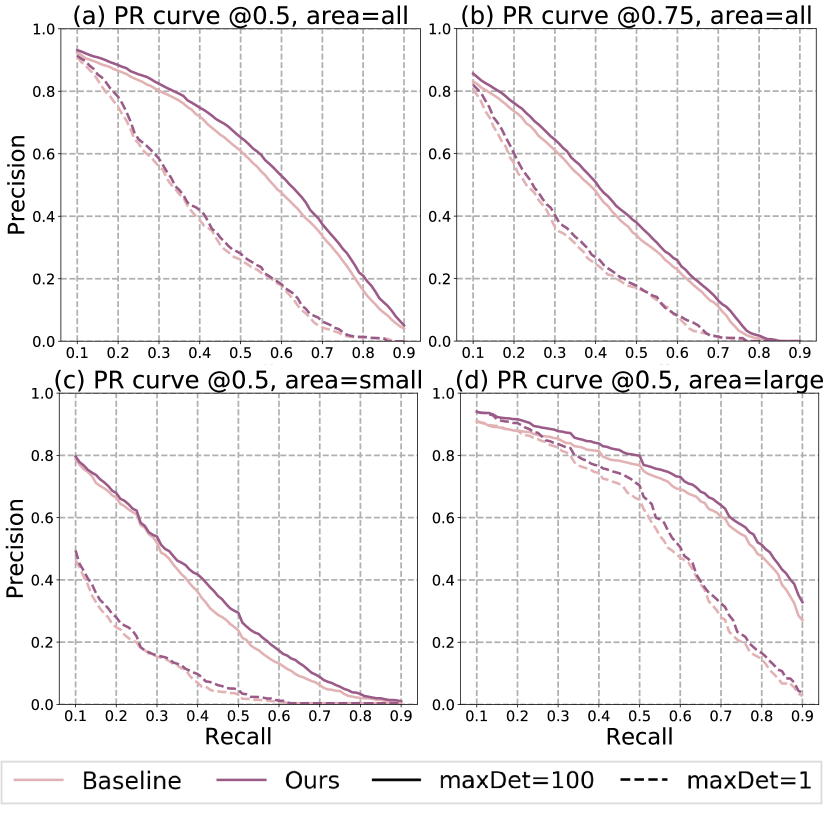
Figure 2: Precision vs. recall (PR) curves of our approach, and comparisons with baselines under different IoU thresholds, object sizes (area) and maximum number of predictions per image (maxDet).

Recall vs. precision.

To better understand how our method improves detection performance, we plot the precision vs. recall curves in Fig 2 and analyze the performance gains. As demonstrated, our method steadily promotes detection performance in different conditions like IoU thresholds, object sizes and maximum number of predictions per image during evaluation. It is also worth noting that our method obtains clear precision gains for all recall ratios, and hence it could be beneficial to various object detection applications in real-world scenarios.

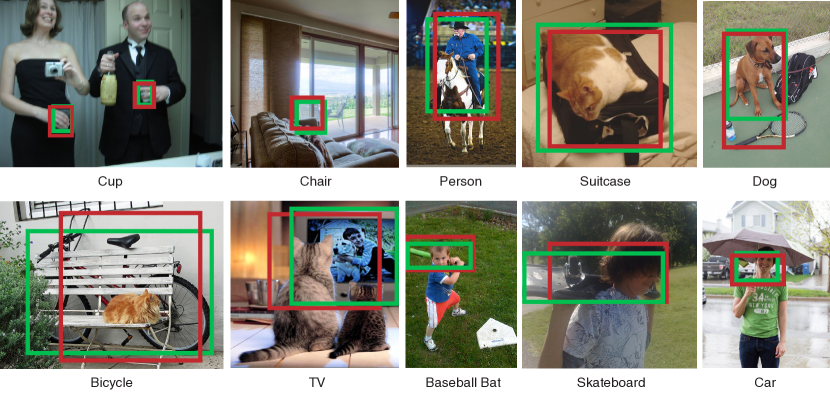
Figure 3: Example candidate boxes (in red) with high IoUs with ground-truth boxes (in green), yet containing noisy contents, are down-weighted by our method. Anchors and ground-truth boxes are denoted in red and green, respectively.

Classification confidence prediction.

We also analyze the predicted classification confidence and investigate whether our proposed method helps alleviate the issue of over confident predictions and reduce the discrepancy between classification prediction and localization accuracy. For baseline detectors and our method, we collect their top-2% confident predictions on COCO minival set before and after NMS and then calculate their mean classification confidence and IoUs with matched ground-truth boxes. As shown in Table 7, detectors trained with our method produces relatively milder predictions than the baseline for classification. Although predictions of the baseline offer a higher average IoU before NMS, it is surpassed by our method after running NMS. This suggests that our method is more friendly when ranking is performed during evaluation since predicted labels are softer and contain more ordering information, and thus is more compatible with NMS. To further verify the ability of our method to correlate classification confidence with localization accuracy, we calculate the Pearson correlation coefficient on these predictions before NMS, and the coefficients between classification confidence and output IoU are 0.169 and 0.194 for baseline and our approach, respectively. This indicates that cleanliness scores considering both branches are able to help bridge the gap between classification and localization.

Method		Before NMS			After NMS
		Mean Conf	Mean IoU		Mean Conf	Mean IoU
Baseline		0.845	0.895		0.958	0.914
Ours		0.782	0.882		0.920	0.921

Table 7: Mean classification confidence and output IoUs with matched ground-truth using predictions before (left) and after NMS (right).

Qualitative analysis.

In addition to quantitative results, we also demonstrate qualitatively in Figure 3 that our method is able to down-weight noisy anchors. As shown in the Figure, our method assigns smaller soft label and re-weighting coefficients to ambiguous samples that contain irrelevant objects or complex background. For example, the anchors encompassing cups in the top-left of Figure 3 are occluded by the lady’s and gentleman’s hands and thus are down-weighted, although they sufficiently overlap with the ground-truth. Similarly, the anchor in the top-middle associated with the person is also down-weighted, since it largely contains irrelevant regions from a horse. This verifies that the label noise can be modeled by our definition of cleanliness and hence are mitigated to improve the training process of object detection. We note that these ambiguous anchors are fairly common—such anchors can be easily found across ten different categories as shown in Figure 3.

6 Conclusion

In this paper, we have presented an approach that is explicitly designed to mitigate noise in anchors used for training object detectors. In particular, we introduced a carefully designed cleanliness score for each anchor used to dynamically adjust their importance during training. These cleanliness scores, leveraging outputs from classification and detection branches, serve as proxies to measure the probability of anchors to be successfully regressed and classified. They are further used as soft supervisory signals to train the classification network and re-weight samples to achieve better localization and classification performance. Extensive studies have been conducted on COCO, and the results demonstrate the effectiveness of the proposed approach both quantitatively and qualitatively.

Acknowledgement HL, ZW and LSD are supported by the Intelligence Advanced Research Projects Activity (IARPA) via Department of Interior/Interior Business Center (DOI/IBC) contract number D17PC00345. The U.S. Government is authorized to reproduce and distribute reprints for Governmental purposes not withstanding any copyright annotation thereon. The views and conclusions contained herein are those of the authors and should not be interpreted as necessarily representing the official policies or endorsements, either expressed or implied of IARPA, DOI/IBC or the U.S. Government.

References

- [1] Devansh Arpit, Stanisław Jastrzębski, Nicolas Ballas, David Krueger, Emmanuel Bengio, Maxinder S Kanwal, Tegan Maharaj, Asja Fischer, Aaron Courville, Yoshua Bengio, et al. A closer look at memorization in deep networks. In ICML, 2017.
- [2] Zhaowei Cai and Nuno Vasconcelos. Cascade r-cnn: High quality object detection and instance segmentation. arXiv preprint arXiv:1906.09756, 2019.
- [3] Yuhang Cao, Kai Chen, Chen Change Loy, and Dahua Lin. Prime sample attention in object detection. arXiv preprint arXiv:1904.04821, 2019.
- [4] Kai Chen, Jiangmiao Pang, Jiaqi Wang, Yu Xiong, Xiaoxiao Li, Shuyang Sun, Wansen Feng, Ziwei Liu, Jianping Shi, Wanli Ouyang, et al. Hybrid task cascade for instance segmentation. In CVPR, 2019.
- [5] Bowen Cheng, Yunchao Wei, Honghui Shi, Rogerio Feris, Jinjun Xiong, and Thomas Huang. Revisiting rcnn: On awakening the classification power of faster rcnn. In ECCV, 2018.
- [6] Jifeng Dai, Yi Li, Kaiming He, and Jian Sun. R-fcn: Object detection via region-based fully convolutional networks. In NeurIPS, 2016.
- [7] Jifeng Dai, Haozhi Qi, Yuwen Xiong, Yi Li, Guodong Zhang, Han Hu, and Yichen Wei. Deformable convolutional networks. In ICCV, 2017.
- [8] Kaiwen Duan, Song Bai, Lingxi Xie, Honggang Qi, Qingming Huang, and Qi Tian. Centernet: Keypoint triplets for object detection. In ICCV, 2019.
- [9] Mark Everingham, Luc Van Gool, Christopher KI Williams, John Winn, and Andrew Zisserman. The pascal visual object classes (voc) challenge. IJCV, 2010.
- [10] Ross Girshick. Fast r-cnn. In CVPR, 2015.
- [11] Ross Girshick, Jeff Donahue, Trevor Darrell, and Jitendra Malik. Rich feature hierarchies for accurate object detection and semantic segmentation. In CVPR, 2014.
- [12] Ross Girshick, Ilija Radosavovic, Georgia Gkioxari, Piotr Dollár, and Kaiming He. Detectron. https://github.com/facebookresearch/detectron, 2018.
- [13] Bo Han, Quanming Yao, Xingrui Yu, Gang Niu, Miao Xu, Weihua Hu, Ivor Tsang, and Masashi Sugiyama. Co-teaching: Robust training of deep neural networks with extremely noisy labels. In NeurIPS, 2018.
- [14] Kaiming He, Xiangyu Zhang, Shaoqing Ren, and Jian Sun. Deep residual learning for image recognition. In CVPR, 2016.
- [15] Lu Jiang, Zhengyuan Zhou, Thomas Leung, Li-Jia Li, and Li Fei-Fei. Mentornet: Learning data-driven curriculum for very deep neural networks on corrupted labels. In ICML, 2017.
- [16] Hei Law and Jia Deng. Cornernet: Detecting objects as paired keypoints. In ECCV, 2018.
- [17] Buyu Li, Yu Liu, and Xiaogang Wang. Gradient harmonized single-stage detector. In AAAI, 2019.
- [18] Junnan Li, Yongkang Wong, Qi Zhao, and Mohan S Kankanhalli. Learning to learn from noisy labeled data. In CVPR, 2019.
- [19] Yanghao Li, Yuntao Chen, Naiyan Wang, and Zhaoxiang Zhang. Scale-aware trident networks for object detection. In ICCV, 2019.
- [20] Yuncheng Li, Jianchao Yang, Yale Song, Liangliang Cao, Jiebo Luo, and Li-Jia Li. Learning from noisy labels with distillation. In CVPR, 2017.
- [21] Tsung-Yi Lin, Piotr Dollár, Ross Girshick, Kaiming He, Bharath Hariharan, and Serge Belongie. Feature pyramid networks for object detection. In CVPR, 2017.
- [22] Tsung-Yi Lin, Priya Goyal, Ross Girshick, Kaiming He, and Piotr Dollár. Focal loss for dense object detection. In ICCV, 2017.
- [23] Tsung-Yi Lin, Michael Maire, Serge Belongie, James Hays, Pietro Perona, Deva Ramanan, Piotr Dollár, and C Lawrence Zitnick. Microsoft coco: Common objects in context. In ECCV, 2014.
- [24] Wei Liu, Dragomir Anguelov, Dumitru Erhan, Christian Szegedy, Scott Reed, Cheng-Yang Fu, and Alexander C Berg. Ssd: Single shot multibox detector. In ECCV, 2016.
- [25] Xin Lu, Buyu Li, Yuxin Yue, Quanquan Li, and Junjie Yan. Grid r-cnn. In CVPR, 2019.
- [26] Jiangmiao Pang, Kai Chen, Jianping Shi, Huajun Feng, Wanli Ouyang, and Dahua Lin. Libra r-cnn: Towards balanced learning for object detection. In CVPR, 2019.
- [27] Junran Peng, Ming Sun, Zhaoxiang Zhang, Tieniu Tan, and Junjie Yan. Pod: Practical object detection with scale-sensitive network. In ICCV, 2019.
- [28] Joseph Redmon and Ali Farhadi. Yolo9000: better, faster, stronger. In CVPR, 2017.
- [29] Mengye Ren, Wenyuan Zeng, Bin Yang, and Raquel Urtasun. Learning to reweight examples for robust deep learning. In ICML, 2018.
- [30] Shaoqing Ren, Kaiming He, Ross Girshick, and Jian Sun. Faster r-cnn: Towards real-time object detection with region proposal networks. In NeurIPS, 2015.
- [31] Abhinav Shrivastava, Abhinav Gupta, and Ross Girshick. Training region-based object detectors with online hard example mining. In CVPR, 2016.
- [32] Bharat Singh, Hengduo Li, Abhishek Sharma, and Larry S Davis. R-fcn-3000 at 30fps: Decoupling detection and classification. In CVPR, 2018.
- [33] Bharat Singh, Mahyar Najibi, and Larry S Davis. Sniper: Efficient multi-scale training. In NeurIPS, 2018.
- [34] Sunil Thulasidasan, Tanmoy Bhattacharya, Jeff Bilmes, Gopinath Chennupati, and Jamal Mohd-Yusof. Combating label noise in deep learning using abstention. In ICML, 2019.
- [35] Zhi Tian, Chunhua Shen, Hao Chen, and Tong He. FCOS: Fully convolutional one-stage object detection. In ICCV, 2019.
- [36] Paul Viola and Michael Jones. Rapid object detection using a boosted cascade of simple features. In CVPR, 2001.
- [37] Jiaqi Wang, Kai Chen, Shuo Yang, Chen Change Loy, and Dahua Lin. Region proposal by guided anchoring. In CVPR, 2019.
- [38] Tong Xiao, Tian Xia, Yi Yang, Chang Huang, and Xiaogang Wang. Learning from massive noisy labeled data for image classification. In CVPR, 2015.
- [39] Saining Xie, Ross Girshick, Piotr Dollár, Zhuowen Tu, and Kaiming He. Aggregated residual transformations for deep neural networks. In CVPR, 2017.
- [40] Philipp Krähenbühl Xingyi Zhou, Dequan Wang. Objects as points. arXiv preprint arXiv:1904.07850, 2019.
- [41] Hongyu Xu, Xutao Lv, Xiaoyu Wang, Zhou Ren, Navaneeth Bodla, and Rama Chellappa. Deep regionlets for object detection. In ECCV, 2018.
- [42] Ze Yang, Shaohui Liu, Han Hu, Liwei Wang, and Stephen Lin. Reppoints: Point set representation for object detection. In ICCV, 2019.
- [43] Hongkai Zhang, Hong Chang, Bingpeng Ma, Shiguang Shan, and Xilin Chen. Cascade retinanet: Maintaining consistency for single-stage object detection. In BMVC, 2019.
- [44] Shifeng Zhang, Longyin Wen, Xiao Bian, Zhen Lei, and Stan Z Li. Single-shot refinement neural network for object detection. In CVPR, 2018.
- [45] Xingyi Zhou, Jiacheng Zhuo, and Philipp Krahenbuhl. Bottom-up object detection by grouping extreme and center points. In CVPR, 2019.
- [46] Chenchen Zhu, Yihui He, and Marios Savvides. Feature selective anchor-free module for single-shot object detection. In CVPR, 2019.