Multimodal Generative Models for Compositional Representation Learning

Abstract

As deep neural networks become more adept at traditional tasks, many of the most exciting new challenges concern multimodality—observations that combine diverse types, such as image and text. In this paper, we introduce a family of multimodal deep generative models derived from variational bounds on the evidence (data marginal likelihood). As part of our derivation we find that many previous multimodal variational autoencoders used objectives that do not correctly bound the joint marginal likelihood across modalities. We further generalize our objective to work with several types of deep generative model (VAE, GAN, and flow-based), and allow use of different model types for different modalities. We benchmark our models across many image, label, and text datasets, and find that our multimodal VAEs excel with and without weak supervision. Additional improvements come from use of GAN image models with VAE language models. Finally, we investigate the effect of language on learned image representations through a variety of downstream tasks, such as compositionally, bounding box prediction, and visual relation prediction. We find evidence that these image representations are more abstract and compositional than equivalent representations learned from only visual data.

1 Introduction

The evidence that reaches our senses is an indirect reflection of complex latent structure in the world. Objects are composed from pieces and substances, they interact with each other in complex ways, and are acted on by agents who have complex goals and beliefs. Because different modalities—vision, touch, sound, language—reflect these latent causes in different ways, models that learn from multiple modalities should yield richer, more abstract, and more generalizable representations. For instance, language is intrinsically compositional, reflecting complex properties and relations. Vision does not directly reflect this structure, spreading the same causes across pixels, but provides far more continuous detail. This suggests the hypothesis that visual representations learned from both visual and linguistic data would reflect the abstract compositional structure of objects more directly. In this paper we explore a new family of multimodal generative models and show that it efficiently learns from complex multimodal data, including from weak supervision, and appears to reflect more abstract and compositional information.

The bulk of previous work on multimodal learning has focused on supervised approaches using deep neural networks (Ngiam et al., 2011; Xu et al., 2015; Liu et al., 2018; Baruch and Keller, 2018). While this family of models can work well, their performance is predicated on large curated datasets of paired examples from different modalities—requiring all the modalities describing each observation to be present. This can be almost impossible in many domains where data is either rare or prohibitively expensive. For example, collecting tactile data requires specialized equipment and is difficult to do at the scale of ImageNet or even COCO. Under these stringent restrictions of data size, supervised multimodal approaches may be suspect to overfitting and poor generalization.

Generative models specialize in un-supervised learning, and deal naturally with missing data (such as missing modalities). There have recently been a number of multimodal generative models (Wang et al., 2016; Suzuki et al., 2016; Vedantam et al., 2017; Wu and Goodman, 2018) built on the variational autoencoder (Kingma and Welling, 2013). Some of these multimodal VAEs enable weakly-supervised learning, where the model only needs a small number of paired examples to learn the “alignment” between different modalities learned by using unpaired data. In many domains it is often the case that while paired examples are expensive, unpaired examples (a single modality) are cheap. For instance, one can find an unlimited amount of unrelated images and text online. However, previous experiments have been limited to straightforward domains with simple images (e.g. MNIST) and labels. These models struggle with richer domains such as natural language or more naturalistic images (e.g. CIFAR). In this paper we argue that there are two reasons for this: the objectives previously used were often not correct bounds on the joint probability, and, individual modalities did not allow strong enough generative models to capture the natural variation in the data.

In this work, we introduce a new family of objectives for multimodal generative models, derived from minimizing variational divergences. We show that many of the previous multimodal VAEs are either special cases of our family or have undesirable objectives that over-emphasize either the marginal or conditional densities. We show that our new multimodal VAE is more stable than and outperforms prior works. Then, to handle richer images (which VAEs notoriously (Zhao et al., 2017a) fail to capture), we show that our multimodal objective is well-defined when individual modalities are parameterized by VAEs, GANs, or invertible flows. Doing so allows us to combine the benefits across these different models: using VAEs for discrete domains such as text and GANs/flows for complex images. We then thoroughly investigate how our family of models performs under weak supervision, varying both the amount of paired and unpaired data. Finally, we explore the representations learned, finding that visual representations co-learned with language are more abstract: they are more compositional and better support transfer tasks of object detection and visual relation prediction.

2 Background

We briefly review popular unimodal generative models.

2.1 Variational Autoencoders

A variational autoencoder (VAE) (Kingma and Welling, 2013; Rezende et al., 2014) specifies a joint distribution $p_{\theta}({\bm{x}},{\bm{z}})=p({\bm{z}})p_{\theta}({\bm{x}}|{\bm{z}})$ over a set of observed variables ${\bm{x}}\in\mathcal{X}$ and stochastic variables ${\bm{z}}\in\mathcal{Z}$ parameterized by $\theta\in\Theta$. The prior, $p({\bm{z}})$ is often isotropic Gaussian whereas the likelihood, $p_{\theta}({\bm{x}}|{\bm{z}})$ is usually Bernoulli for images and Categorical for language. Instead of computing the (intractable) posterior distribution $p_{\theta}({\bm{z}}|{\bm{x}})$, VAEs introduce an approximate posterior $q_{\phi}({\bm{z}}|{\bm{x}})\in\mathcal{Q}$ from a variational family of “simple” distributions that we can score and sample from (e.g. Gaussians). Letting $p_{d}({\bm{x}})$ represent an empirical distribution from which we sample our training dataset, we define a variational joint distribution as $q_{\phi}({\bm{x}},{\bm{z}})=p_{d}({\bm{x}})q_{\phi}({\bm{z}}|{\bm{x}})$. We can interpret VAEs as minimizing the Kullback-Liebler divergence, denoted $D_{\text{KL}}$, between the two joint distributions:

$$D_{\mathrm{KL}}(q_{\phi}({\bm{x}},{\bm{z}})||p_{\theta}({\bm{x}},{\bm{z}})) =\mathbb{E}_{q_{\phi}({\bm{x}},{\bm{z}})}\left[\log\frac{q_{\phi}({\bm{x}},{\bm{z}})}{p_{\theta}({\bm{x}},{\bm{z}})}\right]$$

$$\propto\mathbb{E}_{p_{d}({\bm{x}})}\mathbb{E}_{q_{\phi}({\bm{z}}|{\bm{x}})}\left[\log\frac{q_{\phi}({\bm{z}}|{\bm{x}})}{p_{\theta}({\bm{x}},{\bm{z}})}\right]$$

$$=\mathbb{E}_{p_{d}({\bm{x}})}[-\text{ELBO}({\bm{x}})]$$ (1)

Minimizing Eq. 1 is equivalent to maximizing the evidence lower bound (ELBO) as commonly presented in VAE literature. In practice, $q_{\phi}({\bm{z}}|{\bm{x}})$ and $p_{\theta}({\bm{x}}|{\bm{z}})$ consist of deep neural networks, and Eq. 1 is optimized with stochastic gradient descent using the reparameterization trick to minimize variance when estimating the gradient.

2.2 Generative Adversarial Networks

As elegant as they are, VAEs are not very adept with naturalistic images, as evidenced by blurry samples (Zhao et al., 2017a, b; Gulrajani et al., 2016). In response, newer generative models focus heavily on sample quality. In particular, a generative adversarial network (GAN) (Goodfellow et al., 2014) is a family of deep generative models that learns a deterministic transformation, $f_{\theta}:\mathcal{Z}\rightarrow\mathcal{X}$, on samples from a prior distribution $p({\bm{z}})$ along with an adversarial model trained to distinguish between transformed samples $f_{\theta}({\bm{z}})$ and empirical samples drawn from $p_{d}({\bm{x}})$. The two models are jointly trained in a mini-max game. Unlike VAEs, GANs do not explicitly learn a distribution over ${\bm{x}}$ (i.e. likelihood-free) but allow us to sample from an implicit distribution, $p_{\theta}({\bm{x}}|{\bm{z}})$. As in (Nowozin et al., 2016; Dumoulin et al., 2016), we rewrite the minimax objective as a Fenchel dual of a $f$-divergence (with KL as the metric).

$$D_{\mathrm{KL}}(q_{\phi}({\bm{x}},{\bm{z}})||p_{\theta}({\bm{x}},{\bm{z}})) \geq\sup_{T\in\mathcal{T}}\left(\mathbb{E}_{q_{\phi}({\bm{x}},{\bm{z}})}[T({\bm{x}},{\bm{z}})]-\mathbb{E}_{p_{\theta}({\bm{x}},{\bm{z}})}[e^{T({\bm{x}},{\bm{z}})-1}]\right)$$

$$\geq\sup_{T\in\mathcal{T}_{\psi}}\left(\mathbb{E}_{q_{\phi}({\bm{x}},{\bm{z}})}[T({\bm{x}},{\bm{z}})]-\mathbb{E}_{p_{\theta}({\bm{x}},{\bm{z}})}[e^{T({\bm{x}},{\bm{z}})-1}]\right)$$ (2)

where $p_{\theta}({\bm{x}},{\bm{z}})=p_{\theta}({\bm{x}}|{\bm{z}})p({\bm{z}})$ and $\mathcal{T}$ specifies a class of functions $T:\mathcal{X}\times\mathcal{Z}\rightarrow\mathbb{R}$. This is lower bounded by a smaller class of functions $\mathcal{T}_{\psi}$ parameterized by neural network parameters, $\psi$; we often call $T\in\mathcal{T}_{\psi}$ a discriminator or critic. Like in VAEs, the joint $q_{\phi}({\bm{x}},{\bm{z}})$ is implicitly defined by an empirical distribution $p_{d}({\bm{x}})$ and $q_{\phi}({\bm{z}}|{\bm{x}})$, an approximate inference network. Since we can sample from $p_{\theta}({\bm{x}},{\bm{z}})$ using ${\bm{x}}=f_{\theta}({\bm{z}})$ where ${\bm{z}}\sim p({\bm{z}})$, we can optimize Eq. 2 with SGD and reparameterization.

2.3 Flow-based Models

Flow-based models (Dinh et al., 2016; Papamakarios et al., 2017; Kingma and Dhariwal, 2018; Huang et al., 2018) are another class of generative models that have been shown to work well with naturalistic images. Similar to GANs, flows learn a deterministic transformation $f_{\theta}:\mathcal{Z}\rightarrow\mathcal{X}$ but with the additional constraint that $f_{\theta}$ must be invertible and possess a tractable Jacobian determinant. For example, many flows enforce the Jacobian matrix to be diagonal (Rezende and Mohamed, 2015) or triangular (Dinh et al., 2016) such that the determinant has a closed form expression. Unlike both VAEs and GANs, satisfying these constraints allows us to do exact inference using a change of variables transformation:

$$\log p({\bm{x}})=\log p({\bm{z}})+\log|\det\frac{\partial{\bm{z}}}{\partial{\bm{x}}^{T}}|$$ (3)

where ${\bm{z}}=f_{\theta}^{-1}({\bm{x}})$, and $p({\bm{z}})$ is a simple prior. As a result, generating an observation requires first sampling ${\bm{z}}\sim p({\bm{z}})$, then computing ${\bm{x}}=f_{\theta}({\bm{z}})$. Symmetrically, inference is the opposite: first sample ${\bm{x}}\sim p_{d}({\bm{x}})$, followed by ${\bm{z}}=f_{\theta}^{-1}({\bm{x}})$. Unlike GANs, there is no adversary or additional objective. In practice, $f_{\theta}$ is parameterized by a neural network.

3 Methods

We now introduce a family of multimodal generative models extending the VAE framework presented above. For simplicitly, we restrict to two modalities: Let ${\bm{x}}\in\mathcal{X}$ and ${\bm{y}}\in\mathcal{Y}$ denote observed variables (e.g. images and text) that describe the same natural phenomena. Assume we are given an empirical distribution $p_{d}({\bm{x}},{\bm{y}})$ over paired images and text. Using a latent variable ${\bm{z}}\in\mathcal{Z}$, we define a generative model over the joint distribution that factors as $p_{\theta}({\bm{x}},{\bm{y}},{\bm{z}})=p_{\theta}({\bm{x}}|{\bm{z}})p_{\theta}({\bm{y}}|{\bm{z}})p({\bm{z}})$ where $p({\bm{z}})$ is a prior i.e. ${\bm{x}}\perp{\bm{y}}|{\bm{z}}$. Further, we define three variational posteriors, one for the joint setting $q_{\phi}({\bm{x}},{\bm{y}},{\bm{z}})=p_{d}({\bm{x}},{\bm{y}})q_{\phi}({\bm{z}}|{\bm{x}},{\bm{y}})$, and two for the unimodal cases $q_{\phi}({\bm{x}},{\bm{z}})=p_{d}({\bm{x}})q_{\phi}({\bm{z}}|{\bm{x}})$ and $q_{\phi}({\bm{y}},{\bm{z}})=p_{d}({\bm{y}})q_{\phi}({\bm{z}}|{\bm{y}})$. We note the following property between the joint and unimodal posteriors.

Lemma 1

The multimodal and unimodal posteriors are related by marginalization:

$$\int_{\mathcal{X}}q_{\phi}({\bm{x}},{\bm{y}},{\bm{z}})=q_{\phi}({\bm{y}},{\bm{z}})\quad,\quad\int_{\mathcal{Y}}q_{\phi}({\bm{x}},{\bm{y}},{\bm{z}})=q_{\phi}({\bm{x}},{\bm{z}})$$

Proof  We show the first equality. The second will follow by an identical argument.

$$\int_{\mathcal{X}}q_{\phi}({\bm{x}},{\bm{y}},{\bm{z}}) =\int_{\mathcal{X}}p_{d}({\bm{x}},{\bm{y}})q_{\phi}({\bm{z}}|{\bm{x}},{\bm{y}})=p_{d}({\bm{y}})\int_{\mathcal{X}}p_{d}({\bm{x}}|{\bm{y}})q_{\phi}({\bm{z}}|{\bm{x}},{\bm{y}})$$

$$=p_{d}({\bm{y}})\int_{\mathcal{X}}q_{\phi}({\bm{z}},{\bm{x}}|{\bm{y}})=p_{d}({\bm{y}})q_{\phi}({\bm{z}}|{\bm{y}})=q_{\phi}({\bm{y}},{\bm{z}})$$

 
At first, defining three variational posteriors might seem excessive. Truthfully, the most naive generalization of Eq. 1 to the multimodal setting would only require the joint posterior $q_{\phi}({\bm{x}},{\bm{y}},{\bm{z}})$ by minimizing

$$\mathcal{L}_{0}=D_{\mathrm{KL}}(q_{\phi}({\bm{x}},{\bm{y}},{\bm{z}})||p_{\theta}({\bm{x}},{\bm{y}},{\bm{z}}))$$ (4)

which is a lower bound on $\log p_{\theta}({\bm{x}},{\bm{y}})$ by Jensen’s inequality. However, with a multimodal model, we often want to “translate” between modalities. For instance, we might want to hallucinate conditional images and generate conditional captions. Purely optimizing Eq. 4 does not facilitate such operations as we cannot do inference given a single modality (i.e. missing a modality). To address this, we will need the other two posteriors. We present the following theorem, which decomposes Eq. 4 into a sum of two divergence terms: one for the marginal and one for the conditional.

Theorem 1

Let ${\bm{x}}\in\mathcal{X}$, ${\bm{y}}\in\mathcal{Y}$ be two observed variables, and ${\bm{z}}\in\mathcal{Z}$ be a latent variable. Let $p_{\theta}({\bm{x}},{\bm{y}},{\bm{z}})$ denote a latent variable model parameterizing the joint distribution. Let $q_{\phi}({\bm{x}},{\bm{y}},{\bm{z}})$, $q_{\phi}({\bm{x}},{\bm{z}})$ and $q_{\phi}({\bm{y}},{\bm{z}})$ denote three posteriors over multimodal and unimodal inputs. Define a set of distances between distributions:

$$D_{\alpha} =D_{\mathrm{KL}}(q_{\phi}({\bm{x}},{\bm{z}})||p_{\theta}({\bm{x}},{\bm{z}}))$$

$$D_{\beta} =D_{\mathrm{KL}}(q_{\phi}({\bm{x}},{\bm{y}},{\bm{z}})||q_{\phi}({\bm{x}},{\bm{z}})p_{\theta}({\bm{y}}|{\bm{x}},{\bm{z}}))$$

$$D_{\gamma} =D_{\mathrm{KL}}(q_{\phi}({\bm{y}},{\bm{z}})||p_{\theta}({\bm{y}},{\bm{z}}))$$

$$D_{\eta} =D_{\mathrm{KL}}(q_{\phi}({\bm{x}},{\bm{y}},{\bm{z}})||q_{\phi}({\bm{y}},{\bm{z}})p_{\theta}({\bm{x}}|{\bm{y}},{\bm{z}}))$$

Then, the sum of the distances is equal to twice $\mathcal{L}_{0}$.

$$\mathcal{L}_{\text{M}}=D_{\alpha}+D_{\beta}+D_{\gamma}+D_{\eta}=2\mathcal{L}_{0}$$ (5)

Proof  To show that the statements hold, we need to show both

$$D_{\mathrm{KL}}(q_{\phi}({\bm{x}},{\bm{y}},{\bm{z}})||p_{\theta}({\bm{x}},{\bm{y}},{\bm{z}})) =D_{\mathrm{KL}}(q_{\phi}({\bm{x}},{\bm{z}})||p_{\theta}({\bm{x}},{\bm{z}}))+D_{\mathrm{KL}}(q_{\phi}({\bm{x}},{\bm{y}},{\bm{z}})||q_{\phi}({\bm{x}},{\bm{z}})p_{\theta}({\bm{y}}|{\bm{x}},{\bm{z}}))$$

$$D_{\mathrm{KL}}(q_{\phi}({\bm{x}},{\bm{y}},{\bm{z}})||p_{\theta}({\bm{x}},{\bm{y}},{\bm{z}})) =D_{\mathrm{KL}}(q_{\phi}({\bm{y}},{\bm{z}})||p_{\theta}({\bm{y}},{\bm{z}}))+D_{\mathrm{KL}}(q_{\phi}({\bm{x}},{\bm{y}},{\bm{z}})||q_{\phi}({\bm{y}},{\bm{z}})p_{\theta}({\bm{x}}|{\bm{y}},{\bm{z}}))$$

We show only first equality since the other should be a symmetric argument. We begin by writing the divergence explicitly,

$$D_{\mathrm{KL}}(q_{\phi}({\bm{x}},{\bm{y}},{\bm{z}})||p_{\theta}({\bm{x}},{\bm{y}},{\bm{z}})) =\int_{\mathcal{X}}\int_{\mathcal{Y}}\int_{\mathcal{Z}}q_{\phi}({\bm{x}},{\bm{y}},{\bm{z}})\log\frac{q_{\phi}({\bm{x}},{\bm{y}},{\bm{z}})}{p_{\theta}({\bm{x}},{\bm{y}},{\bm{z}})}d{\bm{z}}d{\bm{y}}d{\bm{x}}$$

$$=\int_{\mathcal{X}}\int_{\mathcal{Y}}\int_{\mathcal{Z}}q_{\phi}({\bm{x}},{\bm{y}},{\bm{z}})\log\frac{q_{\phi}({\bm{x}},{\bm{z}})}{p_{\theta}({\bm{x}},{\bm{z}})}d{\bm{z}}d{\bm{y}}d{\bm{x}}$$

$$\qquad+\int_{\mathcal{X}}\int_{\mathcal{Y}}\int_{\mathcal{Z}}q_{\phi}({\bm{x}},{\bm{y}},{\bm{z}})\log\frac{q_{\phi}({\bm{y}}|{\bm{x}},{\bm{z}})}{p_{\theta}({\bm{y}}|{\bm{x}},{\bm{z}})}d{\bm{z}}d{\bm{y}}d{\bm{x}}$$

$$=D_{1}({\bm{x}},{\bm{y}},{\bm{z}})+D_{2}({\bm{x}},{\bm{y}},{\bm{z}})$$

We consider the two terms separately. We will show that each term can be written as a KL divergence. In the first line, use Lemma. 1 in the second equality.

$$D_{1}({\bm{x}},{\bm{y}},{\bm{z}}) =\int_{\mathcal{X}}\int_{\mathcal{Z}}\log\frac{q_{\phi}({\bm{x}},{\bm{z}})}{p_{\theta}({\bm{x}},{\bm{z}})}(\int_{\mathcal{Y}}q_{\phi}({\bm{x}},{\bm{y}},{\bm{z}})d{\bm{y}})d{\bm{z}}d{\bm{x}}=\int_{\mathcal{X}}\int_{\mathcal{Z}}\log\frac{q_{\phi}({\bm{x}},{\bm{z}})}{p_{\theta}({\bm{x}},{\bm{z}})}q_{\phi}({\bm{x}},{\bm{z}})d{\bm{z}}d{\bm{x}}$$

$$=D_{\mathrm{KL}}(q_{\phi}({\bm{x}},{\bm{z}})||p_{\theta}({\bm{x}},{\bm{z}}))$$

$$D_{2}({\bm{x}},{\bm{y}},{\bm{z}}) =\int_{\mathcal{X}}\int_{\mathcal{Y}}\int_{\mathcal{Z}}q_{\phi}({\bm{x}},{\bm{y}},{\bm{z}})\log\frac{q_{\phi}({\bm{x}},{\bm{y}},{\bm{z}})}{q_{\phi}({\bm{x}},{\bm{z}})p_{\theta}({\bm{y}}|{\bm{x}},{\bm{z}})}d{\bm{z}}d{\bm{y}}d{\bm{x}}$$

$$=D_{\mathrm{KL}}(q_{\phi}({\bm{x}},{\bm{y}},{\bm{z}})||q_{\phi}({\bm{x}},{\bm{z}})p_{\theta}({\bm{y}}|{\bm{x}},{\bm{z}})$$

 
In Thm. 5, we propose $\mathcal{L}_{\text{M}}$ as an objective to optimize a multimodal generative model. It remains to show that Eq. 5 is a valid lower bound on the multimodal evidence, $\log p_{\theta}({\bm{x}},{\bm{y}})$. We do so with the following Corollaries.

Corollary 1

If $q_{\phi}({\bm{z}}|{\bm{y}})$ is a good approximation of $p_{\theta}({\bm{z}}|{\bm{y}})$, then $D_{\beta}\leq\log p_{\theta}({\bm{x}}|{\bm{y}})$. If $q_{\phi}({\bm{z}}|{\bm{x}})$ is a good approximation of $p_{\theta}({\bm{z}}|{\bm{x}})$, then $D_{\eta}\leq\log p_{\theta}({\bm{y}}|{\bm{x}})$.

Proof  We assume that $p_{\theta}({\bm{z}}|{\bm{y}})$ can be substituted by $q_{\phi}({\bm{z}}|{\bm{y}})$.

$$\log p_{\theta}({\bm{x}}|{\bm{y}}) \geq\mathbb{E}_{q_{\phi}({\bm{z}}|{\bm{x}},{\bm{y}})}[\log\frac{p_{\theta}({\bm{x}}|{\bm{z}})p_{\theta}({\bm{z}}|{\bm{y}})}{q_{\phi}({\bm{z}}|{\bm{x}},{\bm{y}})}]=\mathbb{E}_{q_{\phi}({\bm{z}}|{\bm{x}},{\bm{y}})}[\log\frac{p_{\theta}({\bm{x}}|{\bm{z}})q_{\phi}({\bm{z}}|{\bm{y}})}{q_{\phi}({\bm{z}}|{\bm{x}},{\bm{y}})}]$$

$$=\mathbb{E}_{q_{\phi}({\bm{z}}|{\bm{x}},{\bm{y}})}[\log p_{\theta}({\bm{x}}|{\bm{z}})q_{\phi}({\bm{z}}|{\bm{y}})]+D(q_{\phi}({\bm{z}}|{\bm{x}},{\bm{y}})||q({\bm{z}}|{\bm{y}}))$$

$$=D_{\mathrm{KL}}(q_{\phi}({\bm{y}},{\bm{z}})||q_{\phi}({\bm{x}},{\bm{z}})p_{\theta}({\bm{y}}|{\bm{x}},{\bm{z}})))$$

where line 1 follows by assumption and the last line follows by Lemma 2.  
As an immediate consequence, we get the following:

Corollary 2

Given $\mathcal{L}_{\text{M}}$ as defined in Eq. 5, each component is a lower bound on a marginal or conditional distribution:

$$D_{\alpha} \leq\log p_{\theta}({\bm{x}}), D_{\beta}\leq\log p_{\theta}({\bm{y}})$$ (6)

$$D_{\gamma} \leq\log p_{\theta}({\bm{x}}|{\bm{y}}), D_{\eta}\leq\log p_{\theta}({\bm{y}}|{\bm{x}})$$ (7)

Summed together, $\mathcal{L}_{\text{M}}=D_{\alpha}+D_{\beta}+D_{\gamma}+D_{\eta}$, this objective lower bounds double the joint distribution, $2\log p_{\theta}({\bm{x}},{\bm{y}})$.

Proof  Eq. 7 restates Coro. 1. See (Kingma and Welling, 2013) for a proof of Eq. 6.  
Thus, optimizing $\mathcal{L}_{\text{M}}$ optimizes the marginals and conditionals as well as the joint density in a principled manner. If we can explicitly evaluate the likelihoods (e.g. VAE), we can further simplify Thm. 5 into an interpretable form.

Lemma 2

$D_{\alpha},D_{\beta},D_{\gamma},D_{\lambda}$ as defined in Thm. 5 can be written as a sum of four reconstruction terms and four Kullback-Liebner divergence terms.

$$\small D_{\alpha} \propto\mathbb{E}_{p_{d}}[\mathbb{E}_{q_{\phi}({\bm{z}}|{\bm{x}})}[\log p_{\theta}({\bm{x}}|{\bm{z}})]+D_{\mathrm{KL}}(q_{\phi}({\bm{z}}|{\bm{x}})||p({\bm{z}}))]$$ (8)

$$D_{\gamma} \propto\mathbb{E}_{p_{d}}[\mathbb{E}_{q_{\phi}({\bm{z}}|{\bm{y}})}[\log p_{\theta}({\bm{y}}|{\bm{z}})]+D_{\mathrm{KL}}(q_{\phi}({\bm{z}}|{\bm{y}})||p({\bm{z}}))]$$ (9)

$$D_{\beta} \propto\mathbb{E}_{p_{d}}[\mathbb{E}_{q_{\phi}({\bm{z}}|{\bm{x}},{\bm{y}})}[\log p_{\theta}({\bm{x}}|{\bm{z}})]+D_{\mathrm{KL}}(q_{\phi}({\bm{z}}|{\bm{x}},{\bm{y}})||q_{\phi}({\bm{z}}|{\bm{y}}))]$$ (10)

$$D_{\eta} \propto\mathbb{E}_{p_{d}}[\mathbb{E}_{q_{\phi}({\bm{z}}|{\bm{x}},{\bm{y}})}[\log p_{\theta}({\bm{y}}|{\bm{z}})]+D_{\mathrm{KL}}(q_{\phi}({\bm{z}}|{\bm{x}},{\bm{y}})||q_{\phi}({\bm{z}}|{\bm{x}}))]$$ (11)

Proof  Eq. 8, 9 have been shown in Sec. 2.1. We will prove Eq. 10 as the last is symmetric.

$$-D(q_{\phi}({\bm{y}},{\bm{z}})||r_{\phi,\theta}({\bm{x}},{\bm{y}},{\bm{z}})) =-\int_{\mathcal{X}}\int_{\mathcal{Y}}\int_{\mathcal{Z}}q_{\phi}({\bm{x}},{\bm{y}},{\bm{z}})\log\frac{q_{\phi}({\bm{x}},{\bm{y}},{\bm{z}})}{q_{\phi}({\bm{x}},{\bm{z}})p_{\theta}({\bm{y}}|{\bm{x}},{\bm{z}})}d{\bm{z}}d{\bm{y}}d{\bm{x}}$$

$$\propto-\int_{\mathcal{X}}\int_{\mathcal{Y}}p_{d}({\bm{x}},{\bm{y}})\int_{\mathcal{Z}}q_{\phi}({\bm{z}}|{\bm{x}},{\bm{y}})\log\frac{q_{\phi}({\bm{z}}|{\bm{x}},{\bm{y}})}{q_{\phi}({\bm{z}}|{\bm{x}})p_{\theta}({\bm{y}}|{\bm{x}},{\bm{z}})}d{\bm{z}}d{\bm{y}}d{\bm{x}}$$

$$=\mathbb{E}_{p_{d}({\bm{x}},{\bm{y}})}[\int_{\bm{z}}q_{\phi}({\bm{z}}|{\bm{x}},{\bm{y}})\log\frac{q_{\phi}({\bm{z}}|{\bm{x}})p_{\theta}({\bm{y}}|{\bm{x}},{\bm{z}})}{q_{\phi}({\bm{z}}|{\bm{x}},{\bm{y}})}d{\bm{z}}]$$

$$=\mathbb{E}_{p_{d}({\bm{x}},{\bm{y}})}[\mathbb{E}_{q_{\phi}({\bm{z}}|{\bm{x}},{\bm{y}})}[\log p_{\theta}({\bm{x}}|{\bm{z}})]+D(q_{\phi}({\bm{z}}|{\bm{x}},{\bm{y}})||q_{\phi}({\bm{z}}|{\bm{y}}))]$$

where in line 2, we factor out $\frac{p_{d}({\bm{x}},{\bm{y}})}{p_{d}({\bm{x}})}$ as a constant (which should not effect optimization); in line 4 we note $p_{\theta}({\bm{y}}|{\bm{x}},{\bm{z}})=p_{\theta}({\bm{y}}|{\bm{z}})$ since ${\bm{x}}\perp{\bm{y}}|{\bm{z}}$ (consider the graphical stucture for the multimodal VAE).  
The first and third terms in Lemma 2 are standard ELBOs for ${\bm{x}}$ and ${\bm{y}}$. The second and fourth terms each contain a KL divergence term pulling the unimodal variational posterior, $q_{\phi}({\bm{z}}|\cdot)$ closer to the multimodal posterior, $q_{\phi}({\bm{z}}|{\bm{x}},{\bm{y}})$. This intuitively regularizes the inference network when given only one observed modality. For example, minimizing $D_{\mathrm{KL}}(q_{\phi}({\bm{z}}|{\bm{x}},{\bm{y}})||q_{\phi}({\bm{z}}|{\bm{y}}))$ can be interpreted as “do inference as if ${\bm{x}}$ was present when using $q_{\phi}({\bm{z}}|{\bm{y}})$”. One can also interpret this as mapping the unimodal inputs ${\bm{x}}$, ${\bm{y}}$, and multimodal input $({\bm{x}},{\bm{y}})$ to a shared embedding space. Most importantly, we note that by introducing these unimodal inference networks, we can now translate between modalities as desired. For example, we can now sample from ${\bm{y}}\sim p_{\theta}({\bm{y}}|{\bm{z}})$ where ${\bm{z}}\sim q_{\phi}({\bm{z}}|{\bm{x}})$ and vice versa.

3.1 Product of Experts

As presented, the joint variational posterior $q_{\phi}({\bm{z}}|{\bm{x}},{\bm{y}})$ could be a separate neural network with independent parameters with respect to $q_{\phi}({\bm{z}}|{\bm{x}})$ and $q_{\phi}({\bm{z}}|{\bm{y}})$. While this is no doubtedly expressive, it does not scale well to applications with more than two modalities: we would need to define $2^{K}$ inference networks for $K$ modalities, $({\bm{x}}_{1},...,{\bm{x}}_{K})$, which can quickly make learning infeasible. Previous work (Wu and Goodman, 2018; Vedantam et al., 2017) posed an elegant solution to this problem of scalability: define $q_{\phi}({\bm{z}}|{\bm{x}},{\bm{y}})$ as a product of the unimodal posteriors. Precisely, they use a product-of-experts (Hinton, 1999), also called PoE, to relate the true joint posterior to the true unimodal posteriors:

$$p({\bm{z}}|{\bm{x}}_{1},...,{\bm{x}}_{K})\propto\frac{\prod_{i=1}^{K}p({\bm{z}}|{\bm{x}}_{i})}{\prod_{i=1}^{K-1}p({\bm{z}})}\approx\frac{\prod_{i=1}^{K}q({\bm{z}}|{\bm{x}}_{i})p({\bm{z}})}{\prod_{i=1}^{K-1}p({\bm{z}})}=p({\bm{z}})\prod_{i=1}^{K}q({\bm{z}}|{\bm{x}}_{i})$$ (12)

where each true posterior $p({\bm{z}}|{\bm{x}}_{i})$ is approximated by the product distribution $q({\bm{z}}|{\bm{x}}_{i})p({\bm{z}})$, resulting in the product of $K$ experts and a “prior expert” $p({\bm{z}})$.

Given our new multimodal objective function, $\mathcal{L}_{\text{M}}$, we would like to preserve using the PoE for efficient inference. However, it remains to show that under certain assumptions, using the PoE in defining a joint posteriors will converge to the true distribution $p_{\theta}({\bm{z}}|{\bm{x}},{\bm{y}})$.

Theorem 2

Let $p$ denote the true generative model and $q_{\phi}$ denote a variational inference network. If we assume a product-of-experts rule such that $q_{\phi}({\bm{z}}|{\bm{x}},{\bm{y}})=p({\bm{z}})q_{\phi}({\bm{z}}|{\bm{x}})q_{\phi}({\bm{z}}|{\bm{y}})$ and if $q_{\phi}({\bm{z}}|{\bm{x}},{\bm{y}})=p({\bm{z}}|{\bm{x}},{\bm{y}})$ i.e. the true posterior is properly contained in the variational family, then the loss $\mathcal{L}_{\text{M}}=0$.

Proof  To be precise, we make the following assumpmtions:

$$q({\bm{x}},{\bm{y}},{\bm{z}}) =p_{d}({\bm{x}},{\bm{y}})q_{\phi}({\bm{z}}|{\bm{x}},{\bm{y}})$$ (13)

$$q({\bm{z}}|{\bm{x}},{\bm{y}}) =p({\bm{z}}|{\bm{x}},{\bm{y}})=\frac{p({\bm{z}}|{\bm{x}})p({\bm{z}}|{\bm{y}})}{p({\bm{z}})}\cdot\frac{p({\bm{x}})p({\bm{y}})}{p({\bm{x}},{\bm{y}})}\propto\frac{p({\bm{z}}|{\bm{x}})p({\bm{z}}|{\bm{y}})}{p({\bm{z}})}$$ (14)

$$p({\bm{y}}|{\bm{z}},{\bm{x}}) =p({\bm{y}}|{\bm{z}})$$ (15)

where $p_{d}({\bm{x}},{\bm{y}})$ is an empirical distribution. We first observe that $p_{d}(\cdot)=p(\cdot)$ since if $p$ is the true generative model, then any empirical dataset would be sampled from $p$. Then,

$$\mathcal{L}_{\text{M}} =\int_{\mathcal{X}}\int_{\mathcal{Y}}\int_{\mathcal{Z}}q({\bm{x}},{\bm{y}},{\bm{z}})\log\frac{q({\bm{x}},{\bm{z}})p({\bm{y}}|{\bm{x}},{\bm{z}})}{q({\bm{x}},{\bm{y}},{\bm{z}})}d{\bm{z}}d{\bm{y}}d{\bm{x}}$$ (17)

$$=\int_{\mathcal{X}}\int_{\mathcal{Y}}p_{d}({\bm{x}},{\bm{y}})\int_{\mathcal{Z}}q({\bm{z}}|{\bm{x}},{\bm{y}})\log\{\frac{q({\bm{z}}|{\bm{x}})p({\bm{y}}|{\bm{z}})}{q({\bm{z}}|{\bm{x}},{\bm{y}})}\cdot\frac{p_{d}({\bm{x}})}{p_{d}({\bm{x}},{\bm{y}})}\}d{\bm{z}}d{\bm{y}}d{\bm{x}}$$ (18)

$$=\int_{\mathcal{X}}\int_{\mathcal{Y}}p_{d}({\bm{x}},{\bm{y}})\int_{\mathcal{Z}}p({\bm{z}}|{\bm{x}},{\bm{y}})\log\{\frac{p({\bm{z}}|{\bm{x}})p({\bm{y}}|{\bm{z}})}{p({\bm{z}}|{\bm{x}},{\bm{y}})}\cdot\frac{p_{d}({\bm{x}})}{p_{d}({\bm{x}},{\bm{y}})}\}d{\bm{z}}d{\bm{y}}d{\bm{x}}$$ (19)

$$=\int_{\mathcal{X}}\int_{\mathcal{Y}}p_{d}({\bm{x}},{\bm{y}})\int_{\mathcal{Z}}p({\bm{z}}|{\bm{x}},{\bm{y}})\log\{\frac{p({\bm{z}}|{\bm{x}})p({\bm{y}}|{\bm{z}})}{\frac{p({\bm{z}}|{\bm{x}})p({\bm{z}}|{\bm{y}})}{p({\bm{z}})}\cdot\frac{p({\bm{x}})p({\bm{y}})}{p({\bm{x}},{\bm{y}})}}\cdot\frac{p_{d}({\bm{x}})}{p_{d}({\bm{x}},{\bm{y}})}\}d{\bm{z}}d{\bm{y}}d{\bm{x}}$$ (20)

$$=\int_{\mathcal{X}}\int_{\mathcal{Y}}p_{d}({\bm{x}},{\bm{y}})\int_{\mathcal{Z}}p({\bm{z}}|{\bm{x}},{\bm{y}})\log\{\frac{p({\bm{y}}|{\bm{z}})p({\bm{z}})p({\bm{x}},{\bm{y}})}{p({\bm{z}}|{\bm{y}})p({\bm{x}})p({\bm{y}})}\cdot\frac{p_{d}({\bm{x}})}{p_{d}({\bm{x}},{\bm{y}})}\}d{\bm{z}}d{\bm{y}}d{\bm{x}}$$ (21)

$$=\int_{\mathcal{X}}\int_{\mathcal{Y}}p_{d}({\bm{x}},{\bm{y}})\int_{\mathcal{Z}}p({\bm{z}}|{\bm{x}},{\bm{y}})\log\{\frac{p({\bm{x}},{\bm{y}})}{p({\bm{x}})}\cdot\frac{p_{d}({\bm{x}})}{p_{d}({\bm{x}},{\bm{y}})}\}d{\bm{z}}d{\bm{y}}d{\bm{x}}$$ (22)

$$=\int_{\mathcal{X}}\int_{\mathcal{Y}}\int_{\mathcal{Z}}p({\bm{x}},{\bm{y}},{\bm{z}})\log\{1\}d{\bm{z}}d{\bm{y}}d{\bm{x}}$$ (23)

$$=0$$ (24)

We apply Assumption 13,15 in line 18. We apply Assumption 14 in line 19. In line 22, we use the fact $p({\bm{y}}|{\bm{z}})p({\bm{z}})=p({\bm{z}}|{\bm{y}})p({\bm{y}})$. In line 23, we use that $p_{d}(\cdot)=p(\cdot)$.  

Being able to use PoE in our new family of VAEs can be especially important in cases of missing data. We will compare the performance of PoE against specifying a new neural network for $q_{\phi}({\bm{z}}|{\bm{x}},{\bm{y}})$ in our experiments.

4 VAE Experiments

To benchmark our proposed family of models, we first compare against existing multimodal VAEs and supervised baselines on a variety of bimodal datasets involving images and labels. Then, we tackle the challenge of images and language. See supplement for a description of each dataset, the model architectures, and hyperparameters.

4.1 Images and Labels

We transform unimodal image datasets into multimodal ones by treating labels as a second modality (${\bm{x}}$ represents images, ${\bm{y}}$ labels): MNIST, FashionMNIST, CelebA, and CIFAR10. All images are resized to 32 by 32 pixels and all models have identical architectures. For evaluation, we compute the marginal and joint log likelihoods on an unseen test set estimated using 1000 samples (see supplement). In lieu for the conditional probability $p_{\theta}({\bm{y}}|{\bm{x}})$, we compute the classification error of predicting the correct label from an image. We do so by taking $\mu$, the mean of the posterior $q_{\phi}({\bm{z}}|{\bm{x}})$, and decoding to the MAP label from $p_{\theta}({\bm{y}}|{\bm{z}}=\mathbf{\mu})$. Table 1 reports evaluation metrics averaged over 5 runs.

	MNIST			FashionMNIST
Model	$\log p({\bm{x}})$	$\log p({\bm{x}},{\bm{y}})$	Cls. Err.	$\log p({\bm{x}})$	$\log p({\bm{x}},{\bm{y}})$	Cls. Err.
VAE	$-113.26$	-	-	$-299.70$	-	-
Classifier	-	-	$0.984$	-	-	$0.908$
BiVCCA	$-114.15$	-	$\mathbf{0.989}$	$-303.93$	-	$\mathbf{0.915}$
MVAE	$-112.61$	$-113.62$	$0.884$	$\mathbf{-299.19}$	$-299.91$	$0.787$
JMVAE	$-113.81$	$-113.48$	$0.983$	$-301.47$	$-299.91$	$0.900$
VAEVAE	$\mathbf{-112.44}$	$\mathbf{-112.65}$	$0.985$	$-299.21$	$\mathbf{-299.34}$	$0.910$
VAEVAE‡	$-112.78$	$-113.33$	$0.983$	$-299.89$	$-299.64$	$0.906$

	CIFAR10			CelebA
Model	$\log p({\bm{x}})$	$\log p({\bm{x}},{\bm{y}})$	Cls. Err.	$\log p({\bm{x}})$	$\log p({\bm{x}},{\bm{y}})$	Cls. Err.
VAE $\mathbf{-1774.86}$	-	-	$\mathbf{-1582.69}$	-	-
Classifier	-	-	$0.637$	-	-	$\mathbf{0.923}$
BiVCCA	$-1785.33$	-	$\mathbf{0.654}$	$-1596.08$	-	$0.922$
MVAE	$-1775.33$	$-1778.80$	$0.511$	$-1584.25$	$-1588.77$	$0.841$
JMVAE	$-1780.82$	$-1778.27$	$0.541$	$-1595.13$	$-1588.76$	$0.914$
VAEVAE	$-1775.63$	$\mathbf{-1777.25}$	$0.607$	$-1584.31$	$\mathbf{-1586.92}$	$0.920$
VAEVAE‡	$-1776.71$	$-1778.45$	$0.601$	$-1586.95$	$-1587.20$	$0.918$

Table 1: Evaluation of Multimodal VAEs on Image and Label Datasets. We also include a supervised baseline (Classifier) and an image-only generative model (VAE). The model VAEVAE^‡ uses Product-of-Experts in the variational posterior. All models share the same architecture and hyperparameters. To evaluate each of the models, we compare log probabilities of test data and approximate conditional distributions by classification error (Cls. Err.) on test data.

	MNIST Math				Chairs in Context
Model	$\log p({\bm{x}})$	$\log p({\bm{y}})$	$\log p({\bm{x}},{\bm{y}})$	Perp.	$\log p({\bm{x}})$	$\log p({\bm{y}})$	$\log p({\bm{x}},{\bm{y}})$	Perp.
VAE (${\bm{x}}$)	$-113.21$	-	-	-	$\mathbf{-592.6}$	-	-	-
VAE (${\bm{y}}$)	-	$-0.143$	-	-	-	$-10.8$	-	-
Captioner	-	-	-	$2.231$	-	-	-	$\mathbf{1.7e3}$
BiVCCA	$-114.81$	$-0.193$	-	$\mathbf{2.196}$	$-601.2$	$-10.9$	-	$2.5e4$
MVAE	$\mathbf{-112.62}$	$-0.141$	$-113.72$	$1.6e4$	$-607.9$	$-10.8$	$-636.2$	$1.5e6$
JMVAE	$-115.73$	$-0.410$	$-114.00$	$9.5e3$	$-638.0$	$-13.3$	$-619.7$	$4.8e6$
VAEVAE	$-112.88$	$\mathbf{-0.133}$	$\mathbf{-113.03}$	$745.2$	$-602.3$	$-10.5$	$\mathbf{-619.5}$	$1.7e5$
VAEVAE‡	$-113.41$	$-0.133$	$-113.69$	$274.0$	$-602.3$	$\mathbf{-10.4}$	$-620.6$	$8.2e5$

	Flickr30k				COCO Captions
Model	$\log p({\bm{x}})$	$\log p({\bm{y}})$	$\log p({\bm{x}},{\bm{y}})$	Perp.	$\log p({\bm{x}})$	$\log p({\bm{y}})$	$\log p({\bm{x}},{\bm{y}})$	Perp.
VAE (${\bm{x}}$)	$-1772.8$	-	-	-	$\mathbf{-1769.5}$	-	-	-
VAE (${\bm{y}}$)	-	$-65.1$	-	-	-	$-14.3$	-	-
Captioner	-	-	-	$170.4$	-	-	-	$\mathbf{121.2}$
BiVCCA	$-1883.8$	$-65.4$	-	$\mathbf{153.9}$	$-1778.4$	$-14.9$	-	$133.8$
MVAE	$\mathbf{-1781.0}$	$-65.8$	$-1943.3$	$4.7e5$	$-1778.4$	$-14.5$	$-1875.9$	$3.6e6$
JMVAE	$-1967.2$	$-75.9$	$-1872.9$	$1.6e4$	$-2028.8$	$-21.7$	$-1823.3$	$4.3e9$
VAEVAE	$-1804.8$	$\mathbf{-64.4}$	$\mathbf{-1825.1}$	$7.7e3$	$-1786.8$	$\mathbf{-14.1}$	$\mathbf{-1818.7}$	$3.2e4$
VAEVAE‡	$-1814.2$	$-65.2$	$-1850.2$	$7.6e3$	$-1806.4$	$-14.1$	$-1834.5$	$6.5e4$

Table 2: Evaluation of Multimodal VAEs on Image and Text Datasets. We include a supervised captioning model (Captioner) and two unimodal generative models (VAE ($\mathbf{x}$), VAE ($\mathbf{y}$)). The model VAEVAE^‡ uses Product-of-Experts in the variational posterior. All models share the same architecture and hyperparameters. To evaluate each of the models, we compare log probabilities of test data and approximate conditional distributions by the perplexity of captions conditioned on the image (perp.) using test data.

Results

Previous multimodal models either bias towards capturing marginal or conditional distributions. In fact, many of their objective functions fail to lower bound one or the other (see Sec. 9). In Table 1, we find that BiVCCA and JMVAE have lower (more negative) marginal and joint log-likelihoods than other models, only doing well in classification error (conditionals). On the other hand, MVAE is the opposite, resulting in poor classification and overfitting to the marginals. However, our class of generative models (VAEVAE), which has a principled lower bound, finds a good balance between learning marginals versus conditionals. In all four datasets, VAEVAE does better than BiVCCA and JMVAE in capturing $\log p({\bm{x}})$ and $\log p({\bm{x}},{\bm{y}})$, almost matching the performance of a unimodal VAE. Furthermore, VAEVAE outperforms MVAE in classification, nearing supervised models. Finally, we find that VAEVAE with PoE, denoted by VAEVAE^‡, closely approximates the standard VAEVAE, suggesting that we can trade a little performance for the efficiency that comes with PoE.

4.2 Images and Text

Many prior work in multimodal generative models (Wang et al., 2016; Suzuki et al., 2016; Vedantam et al., 2017; Wu and Goodman, 2018) only testing their methods against simple images and labels (as above). However, we would expect many more benefits to multimodal learning given two rich modalities. So in these next set of experiments, we apply our method to four datasets with images (${\bm{x}}$) and language (${\bm{y}}$). The first is a toy setting based on MNIST where we procedurally generate math equations that evaluate to a digit in the dataset. The second is the “Chairs In Context“ (CIC) dataset (Achlioptas et al., 2018), which contains 80k human utterances paired with images of chairs from ShapeNet (Chang et al., 2015). The final two are Flickr30k (Plummer et al., 2015) and COCO captions (Chen et al., 2015), which contain richer images and text. Like above, we evaluate models with estimates of marginal $\log p_{\theta}({\bm{x}})$, $\log p_{\theta}({\bm{y}})$ and joint $\log p_{\theta}({\bm{x}},{\bm{y}})$ log probabilities with respect to a test set. Instead of classification, we measure the (conditional) perplexity of ${\bm{y}}$ given ${\bm{x}}$ as a surrogate for $\log p_{\theta}({\bm{y}}|{\bm{x}})$, which is difficult to directly estimate. A better generative model should have lower perplexity, or less surprisal for every word in a sentence. To encode and decode utterances, we use RNNVAEs (Bowman et al., 2015). Table 2 compare model performances. For baselines, we include a supervised captioning model and two VAEs, one exclusively for images and one exclusively for text. Once again, all models share architectures and hyperparameters, meaning that any differences in metrics are due to the objectives alone.

Results

We find similar patterns as described for image and label datasets, although the magnitude of the effect is higher for image and text. As before, JMVAE has poor performance in marginal and joint probabilities whereas MVAE has poor (conditional) perplexity. Our VAEVAE models often matches the MVAE in $\log p_{\theta}({\bm{x}})$, $\log p_{\theta}({\bm{y}})$, and $\log p_{\theta}({\bm{x}},{\bm{y}})$ and surpasses JMVAE in perplexity. From Table 2, we can see that supervised approaches like a captioner or BiVCCA tend to do far better in perplexity due to heavily overfitting to learning only the mapping from image to text, a much lower dimensional transformation than learning a full joint representation. But out of the joint generative models, VAEVAE outperforms others by orders of magnitude in perplexity. If a practitioner only cared about image captioning, he/she should use a supervised model. But as we will explore in the next section, in cases of missing data or low supervision, discriminative approaches quickly deteriorate. We will show how VAEVAE is able to leverage unpaired marginal data to still learn a good joint representation under data scarcity.

5 Weak Supervision

In many contexts, it is infeasible to curate a large dataset of paired modalities (e.g. matching image and text), especially as the number of modalities increase. Often, we only have the resources to build a very small set of paired examples. However, unimodal (or unpaired) data is easily accessible both from existing corpora like ImageNet (Russakovsky et al., 2015) or the Google Books corpus (Michel et al., 2011) and from scraping online content from Wikipedia or Google Images. One of the strengths of some generative models (in comparison to a supervised one) is the ability to do inference and make predictions despite missing data. As such, we might wish to use unpaired examples to thoroughly capture marginal distributions whereas existing paired examples can be used to align unimodal representations into a joint space. For the VAEVAE, since $\mathcal{L}_{M}$ is composed of two marginal and two conditional terms, we must use paired examples to evaluate the latter but are free to use unpaired examples to evaluate the former. Wu and Goodman (2018) began to investigate using unpaired examples to training the MVAE. Here, we continue with more thorough experiments where we reserve a fraction of a dataset to be paired and randomly scramble the remaining examples to remove alignment. We vary the fraction of paired examples to gauge how increased amounts of “supervision” effects training. Then, using a fixed amount of supervision, we vary the amount of unpaired examples to test if learning marginal distributions better can make joint representation learning easier.

5.1 Varying Amount of Paired Data

First we vary the amount of paired examples from 0.1% to 100% of the training dataset size. For each setting, we track classification accuracy for labelled datasets and conditional perplexity for image and text datasets. Only VAEVAE and MVAE can make use of unpaired data. All other baseline models only train on the supervised fraction.

Fig. 1(a-d) plot the classification accuracy against log of the supervision percentage (higher is better). We find VAEVAE to consistently do better in the low supervision regime (-2 to 0 log supervision). However as we approach full supervision, the supervised baseline and BiVCCA tend to outperform VAEVAE. Given enough paired data, this is expected as it is much easier to learn $p({\bm{y}}|{\bm{x}})$ alone rather the marginals, conditionals, and joint altogether. Fig. 1(e-h) show the marginal (log) densities over images in each dataset. Again we find VAEVAE to outperform most models, occasionally being beat by the MVAE. Fig. 2 show similar findings to Fig. 1 but for image and text datasets. Fig. 2(a-d) plot the log perplexity of observed text conditioned on the image (lower is better) against log supervision percentage; Fig. 2(e-h) each contain two plots (the left representing the marginal log densities for image and the right for text). The patterns are the same: VAEVAE does the best at low supervision levels and captures the marginal distributions nicely. These patterns lay bare evidence that (1) MVAE over-prioritizes the marginals as it consistently achieves the lowest accuracy under low supervision, (2) JMVAE over-prioritizes the conditionals as it consistently gets the lowest marginal log likelihood, and (3) VAEVAE achieves a good balance between the two.

5.2 Varying Amount of Unpaired Data

Using more unpaired data should help models better capture marginal distributions. We hypothesize that this could make learning the joint and conditional distributions easier as well: Imagine that the joint representation is a “simple” transformation from the unimodal representations; if we learn the latter well, any existing supervision can be used to learn that transformation. To test this intuition, we fix the amount of supervision to 1% and vary the amount of unpaired data (for each modality) from 0.1% to 100%. Again, only VAEVAE and MVAE can make use of unpaired data.

Fig. 3 show the effects on classification accuracy (a), conditional perplexity (b), and marginal log-likelihoods (c,d) as more unpaired data is given to the model. With little unpaired data, performance suffers greatly as generative models struggle to learn the underlying structure in the data distribution, leading to worse performance than a supervised baseline. But as the amount of unpaired data increases, classification error and conditional perplexity steadily decrease, beating the supervised baseline. Since unpaired data comes from the same distribution as paired data, more of it consistently leads to increased performance across datasets.

6 Generalization to Other Model Families

Thm. 5 as stated, is not restricted to VAEs. In this section, we generalize the multimodal objective to GANs and flows.

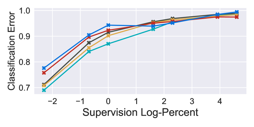
(a) MNIST

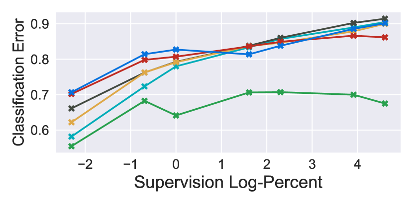
(b) FashionMNIST

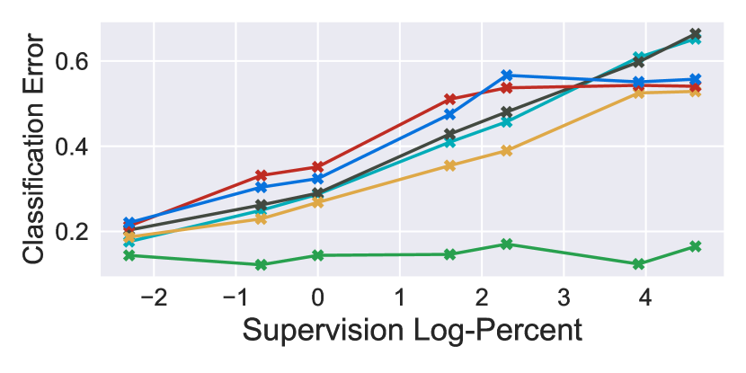
(c) CIFAR10

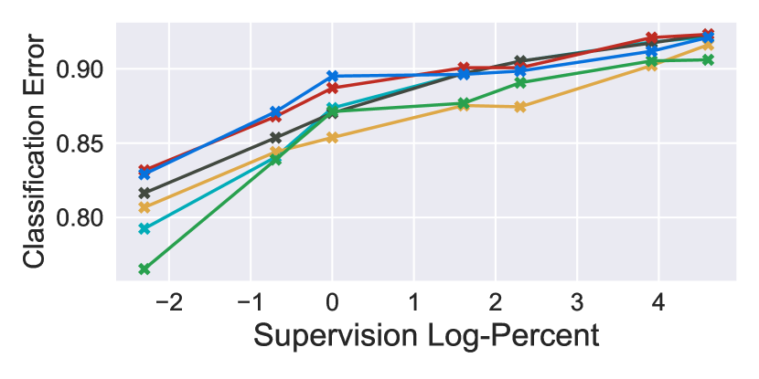
(d) CelebA

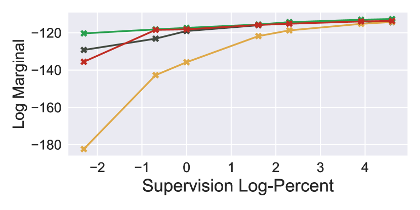
(e) MNIST

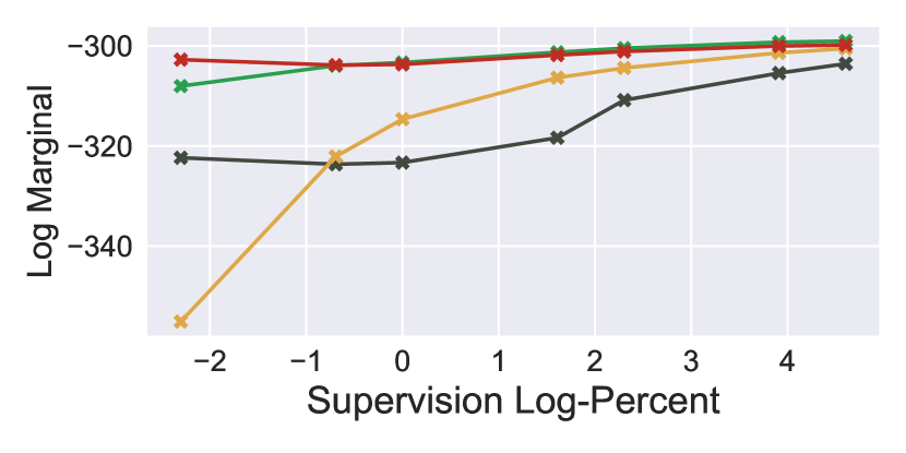
(f) FashionMNIST

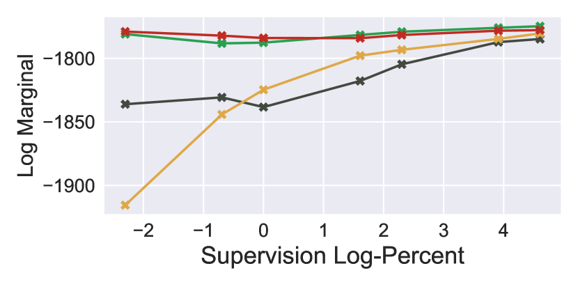
(g) CIFAR10

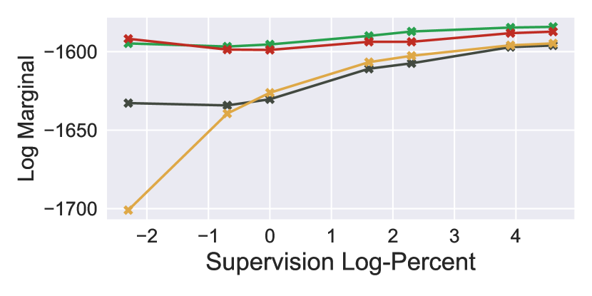
(h) CelebA

Figure 1: Effect of weak supervision on classification (a-d) and marginal density (e-h). Our proposed models have higher accuracy in low to medium supervision. Being able to use unpaired examples ensures much better density estimation. All results are averaged over 3 runs.

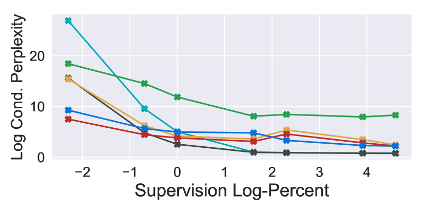
(a) MNIST-Math

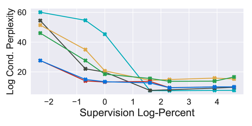
(b) CIC

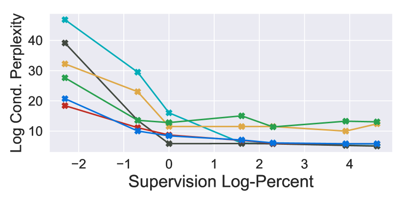
(c) Flickr30k

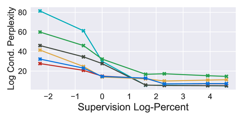
(d) COCO

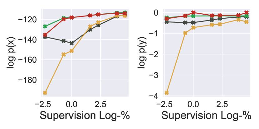
(e) MNIST-Math

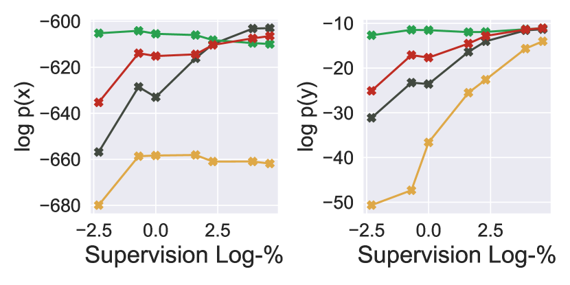
(f) CIC

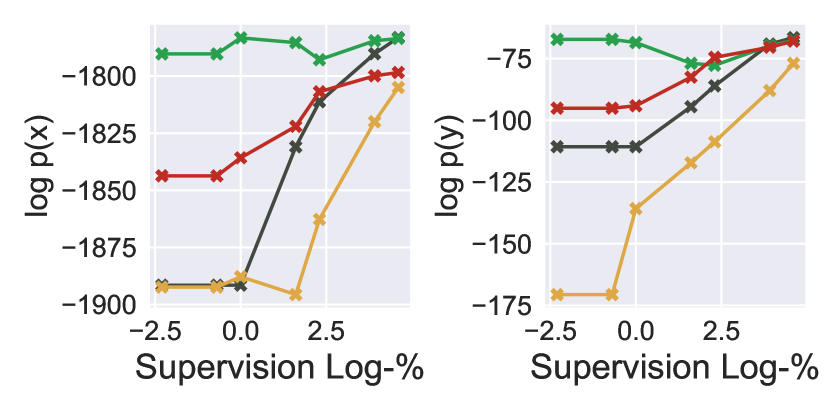
(g) Flickr30k

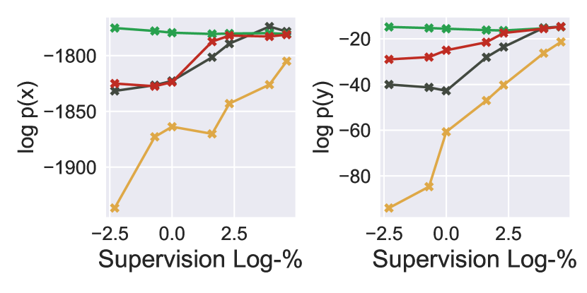
(h) COCO

Figure 2: Effect of weak supervision on conditional perplexity (a-d) and marginal densities for image and text (e-h). VAEVAE uses unpaired data to learn conditional and marginal distributions, contributing to its strong performance.

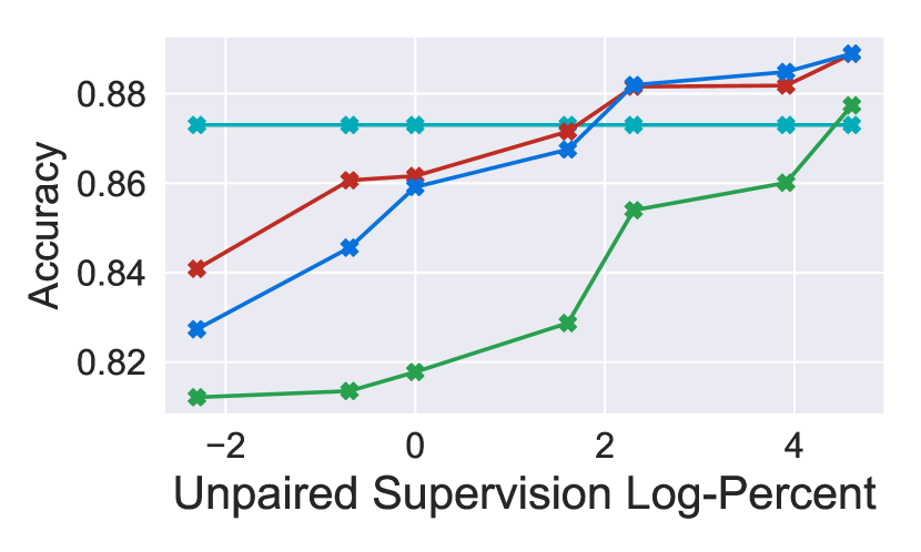
(a) CelebA

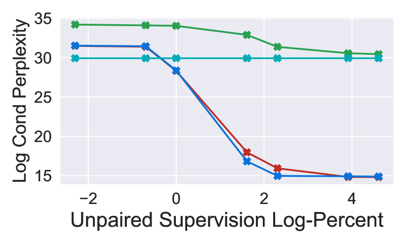
(b) COCO

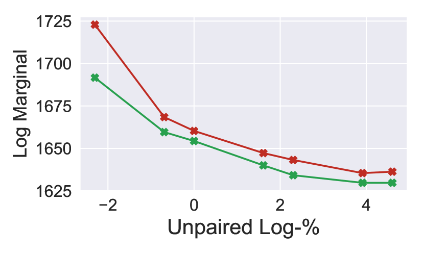
(c) CelebA

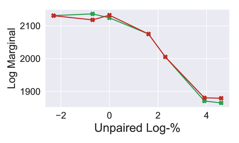
(d) COCO

Figure 3: Effect of unpaired data on conditional prediction (a,b) and marginal (image) density estimation (c,d). Since supervised baseline is unable to use unpaired data, it is constant. The amount of paired supervision is at 1% for all experiments here.

6.1 Multimodal VAEGANs

Recall in Sec. 2.2, we showed that a KL divergence can be rewritten as a supremum over the difference of two expectation terms. As $\mathcal{L}_{\text{M}}$ is composed of four KL divergences, we can replace any of four terms with its Fenchel dual. For example, the divergence between two multimodal distributions can be lower bounded by

$$D_{\mathrm{KL}}(q_{\phi}({\bm{x}},{\bm{y}},{\bm{z}})||r({\bm{x}},{\bm{y}},{\bm{z}}))\geq\sup_{S\in\mathcal{S}}\{\mathbb{E}_{q_{\phi}({\bm{x}},{\bm{y}},{\bm{z}})}[S({\bm{x}},{\bm{y}},{\bm{z}})]-\log\mathbb{E}_{r({\bm{x}},{\bm{y}},{\bm{z}})}[e^{S({\bm{x}},{\bm{y}},{\bm{z}})-1}]\}$$ (25)

where $r({\bm{x}},{\bm{y}},{\bm{z}})=q_{\phi}({\bm{x}},{\bm{z}})p_{\theta}({\bm{y}}|{\bm{x}},{\bm{z}})$ and $\mathcal{S}=\{S:\mathcal{X}\times\mathcal{Y}\times\mathcal{Z}\rightarrow\mathbb{R}\}$ specifies a family of multimodal functions analogous to the discriminator $\mathcal{T}$ from Eq. 2. We arrive at similar definitions for the other terms in Thm. 5. Drawing from (Dumoulin et al., 2016), $q_{\phi}({\bm{z}}|{\bm{x}},{\bm{y}})$, $q_{\phi}({\bm{z}}|{\bm{x}})$, and $q_{\phi}({\bm{z}}|{\bm{y}})$ are adversarially learned inference (ALI) networks, commonly Gaussian posteriors. Sampling from the joint $q_{\phi}({\bm{x}},{\bm{y}},{\bm{z}})$ amounts to sampling ${\bm{z}}\sim q_{\phi}({\bm{z}}|{\bm{x}},{\bm{y}})$ with ${\bm{x}},{\bm{y}}\sim p_{d}({\bm{x}},{\bm{y}})$, the empirical distribution. Similarly, sampling from the product $q_{\phi}({\bm{x}},{\bm{z}})p_{\theta}({\bm{y}}|{\bm{x}},{\bm{z}})$ amounts to sampling ${\bm{z}}\sim q_{\phi}({\bm{z}}|{\bm{x}})$ with ${\bm{x}}\sim p_{d}({\bm{x}})$ and ${\bm{y}}\sim p_{\theta}({\bm{y}}|{\bm{z}})$. As everything is reparameterizable, we can optimize with SGD. This allows us to define a multimodal objective by replacing any of terms in $\mathcal{L}_{\text{M}}$ with its dual. By doing so, we no longer explicitly model the likelihood term $p_{\theta}(\cdot|{\bm{z}})$, but expect improved sample quality.

Lipschitz Constraint

GANs are known to struggle with mode collapse, where generated samples have low variety, memorizing individual images from the training dataset. In practice, we find this to be even more problematic in the multimodal domain. Wasserstein GANs (WGAN) (Arjovsky et al., 2017; Gulrajani et al., 2017) have been presented as a possible solution where instead of a variational divergence, the model minimizes the earth mover (EM) distance between the generative and empirical distributions. EM distance has its own dual representation that restricts the discriminator to be 1-Lipschitz, a constraint that prevents a discriminator from overpowering the generator, helping deter mode collapse Arjovsky et al. (2017). Unfortunately, EM is not directly applicable to our family of objectives. However, using the VAEGAN as presented would indeed face mode collapse issues.

We propose a simple amendment inspired by WGAN: add a 1-Lipschitz constraint on the class of functions, $\mathcal{T}$ and $\mathcal{S}$ in Eq. 25. We note that this is still well-defined,

$$D_{\mathrm{KL}}(q_{\phi}({\bm{x}},{\bm{z}})||p_{\theta}({\bm{x}},{\bm{z}})) \geq\sup_{T\in\mathcal{T}}\{\mathbb{E}_{q_{\phi}({\bm{x}},{\bm{z}})}[T({\bm{x}},{\bm{z}})]-\log\mathbb{E}_{p_{\theta}({\bm{x}},{\bm{z}})}[e^{T({\bm{x}},{\bm{z}})-1}]\}$$ (26)

$$\geq\sup_{T\in\mathcal{T}_{1}}\{\mathbb{E}_{q_{\phi}({\bm{x}},{\bm{z}})}[T({\bm{x}},{\bm{z}})]-\log\mathbb{E}_{p_{\theta}({\bm{x}},{\bm{z}})}[e^{T({\bm{x}},{\bm{z}})-1}]\}$$ (27)

where $\mathcal{T}_{1}$ represents a class of 1-Lipschitz functions. Notably, $\mathcal{T}_{1}\subseteq\mathcal{T}$, meaning that the Eq. 26 is lower bounded by Eq. 27. Thus, Eq. 27 is still a lower bound on the original divergence. We can similarly define $\mathcal{S}_{1}\subseteq\mathcal{S}$ for the multimodal discriminator. Fig. 4 shows the effect of the Lipschitz constraint on sample quality for VAEGANs. Surprisingly, we find the constraint to reduce mode collapse and improve alignment between modalities.

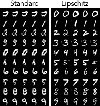
(a) MNIST

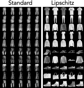
(b) FashionMNIST

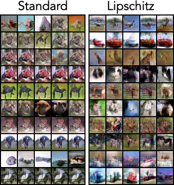
(c) CIFAR10

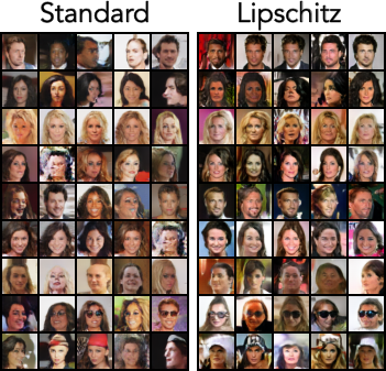
(d) CelebA

Figure 4: Conditional samples from a VAEGAN for each label with and without the Lipschitz constraint. Without the constraint, we see evidence of mode collapse (repetitive images) and incorrect samples for certain classes (e.g. digits 4 and 5 in MNIST or all of FashionMNIST).

6.2 Multimodal VAE-Flows

As flow models do exact inference, there is no need to use variational methods. But we can still decompose a multimodal flow model into a marginal and conditional component, namely

$$\log p_{\theta}({\bm{x}},{\bm{y}}) =\log p_{\theta}({\bm{x}})+\log p_{\theta}({\bm{y}}|{\bm{x}})$$ (28)

$$=\log p_{\theta}({\bm{y}})+\log p_{\theta}({\bm{x}}|{\bm{y}})$$ (29)

Sec. 2.3 showed how to parameterize the marginal terms by defining a deterministic transformation $f_{\theta}:\mathcal{X}\rightarrow\mathcal{Z}$. We can do something similar for the conditional term:

$$\log p_{\theta}({\bm{x}}|{\bm{y}}) =\log p_{\theta}({\bm{z}}|{\bm{y}})+\log|\det\frac{\partial{\bm{z}}}{\partial{\bm{x}}^{T}}|$$ (30)

$$\approx\log q_{\phi}({\bm{z}}|{\bm{y}})+\log|\det\frac{\partial{\bm{z}}}{\partial{\bm{x}}^{T}}|$$ (31)

where ${\bm{z}}=g_{\theta}({\bm{x}})$ for a new “flow” function $g:\mathcal{X}\rightarrow\mathcal{Z}$ parameterized by a neural network. Note that $g_{\theta}(\cdot)$ and $f_{\theta}(\cdot)$ are two distinct models and do not share parameters. In Eq. 31, we replaced the true (intractable) posterior with a variational approximation. Similarly, we can learn transformations for $\log p_{\theta}({\bm{x}}|{\bm{y}})$. In practice, we use real-valued non-volume preserving transforms, or real NVP (Dinh et al., 2014, 2016). These models design their flow functions using affine coupling layers, which enforces the Jacobian matrix to be triangular, thereby making the determinant tractable. We will denote these multimodal models as VAENVP. Future work could explore using recently proposed flows like Glow (Kingma and Dhariwal, 2018) or FFJORD (Grathwohl et al., 2018).

7 VAEGAN and VAENVP Experiments

We conduct several experiments using VAEs, GANs, or NVPs to capture image modalities whereas label and text, being discrete, requires VAEs. With these new hybrid models, we focus on improved sample generation, especially for naturalistic images.

7.1 Evaluation

There is a lack of consistent high-quality metrics for sample generation, so we settle for a few heuristics. As in previous work, we compute the Frenet Inception distance (FID) (Salimans et al., 2016) between generated image samples and observations from the training datset. FID is defined as

$$\text{FID}=||\mu_{r}-\mu_{g}||^{2}+\text{Tr}(\Sigma_{r}+\Sigma_{g}-2(\Sigma_{r}\Sigma_{g})^{\frac{1}{2}})$$ (32)

where $\mu_{r},\Sigma_{r}$ are the mean and covariance of activations from an intermediate layer of a deep neural network (we call this an “oracle” network) given inputs ${\bm{x}}\sim p_{d}({\bm{x}})$. The variables $\mu_{g},\Sigma_{g}$ are similarly computed using inputs ${\bm{x}}\sim p_{\theta}({\bm{x}}|{\bm{z}})$. Previous work use Inception (Szegedy et al., 2015) trained on ImageNet to compute FID. In practice, we do not find it appropriate to use the same network on all datasets (e.g. Inception on MNIST), especially ones very different in distribution and content than ImageNet. Instead, we train our own supervised network specific to each dataset to compute FID. This implies that while our FID can be compared across models for a single dataset, it cannot be compared across datasets. Specifically, we use a dual path network (DPN) (Chen et al., 2017) as the oracle for image and label datasets. Since nothing restricts FID from being used for image and text datasets, we pull statistics from an intermediate layer from a trained captioner with visual attention (Xu et al., 2015). In all settings, we compute FID using 50k samples.

Given an oracle network, we can separately use it classify or caption conditionally sampled images from a multimodal generative model. For instance, given a generated image of a MNIST digit with label 9, we can use the oracle to classify the image. Assuming the oracle is a “perfect” classifier, a better generative model would produce samples that can be classified correctly. A perfect generator would achieve a score of 1. Likewise, for image and text datasets, a perfect generator should achieve very low perplexity as scored by the oracle. We call this metric the oracle sampling error or OSE. In short, FID is a measure of marginal sample quality whereas OSE is a measure of conditional sample quality.

	MNIST		FashionMNIST		CIFAR10		CelebA
Model	FID	OSE	FID	OSE	FID	OSE	FID	OSE
VAE	$1.31$	-	$1.35$	-	$8.48$	-	$8.86$	-
GAN	$1.77$	-	$\mathbf{1.32}$	-	$\mathbf{2.35}$	-	$\mathbf{3.39}$	-
GAN§	$1.87$	-	$2.24$	-	$3.03$	-	$4.19$	-
NVP	$2.17$	-	$5.01$	-	$3.86$	-	$5.05$	-
CVAE	-	$0.91$	-	$0.82$	-	$0.18$	-	$0.89$
CGAN	-	$0.95$	-	$0.71$	-	$0.39$	-	$0.89$
BiVCCA	$4.41$	$0.90$	$5.51$	$0.75$	$8.88$	$0.09$	$18.2$	$0.90$
MVAE	$1.60$	$0.64$	$1.43$	$0.53$	$8.42$	$0.11$	$9.09$	$0.83$
JMVAE	$2.60$	$0.80$	$1.79$	$0.74$	$8.61$	$0.18$	$8.61$	$0.87$
VAEVAE	$1.88$	$0.89$	$1.68$	$0.77$	$8.48$	$0.15$	$8.53$	$0.89$
VAEVAE‡	$1.76$	$0.89$	$1.67$	$0.76$	$8.51$	$0.16$	$8.89$	$0.90$
VAEGAN	$12.8$	$0.50$	$35.7$	$0.10$	$5.92$	$0.34$	$18.7$	$0.89$
VAEGAN‡	$11.4$	$0.59$	$19.2$	$0.37$	$3.13$	$0.37$	$13.7$	$0.88$
VAEGAN§	$\mathbf{0.40}$	$\mathbf{0.99}$	$1.44$	$\mathbf{0.93}$	$2.80$	$\mathbf{0.44}$	$4.07$	$\mathbf{0.93}$
VAENVP	$3.14$	$0.94$	$4.59$	$0.76$	$4.13$	$0.32$	$5.71$	$\mathbf{0.93}$

	MNIST Math		CIC		Flickr30k		COCO
Model	FID	OSE	FID	OSE	FID	OSE	FID	OSE
VAE	$4.68$	-	$20.3$	-	$2.7e2$	-	$3.3e2$	-
GAN	$3.60$	-	$6.88$	-	$88.8$	-	$53.2$	-
GAN§	$3.75$	-	$7.21$	-	$1.6e2$	-	$1.3e2$	-
NVP	$6.44$	-	$13.0$	-	$88.9$	-	$80.9$	-
CVAE	-	$4.1e4$	-	$5e13$	-	$2.6e7$	-	$1.8e10$
CGAN	-	$3.5e4$	-	$3e13$	-	$1.2e7$	-	$4.9e9$
BiVCCA	$4.62$	$3.7e4$	$38.2$	$3e11$	$3.0e2$	$5.8e6$	$3.9e2$	$1.5e10$
MVAE	$4.18$	$4.0e4$	$25.0$	$2e13$	$3.5e2$	$4.3e7$	$4.6e2$	$1.3e10$
JMVAE	$4.39$	$3.9e4$	$45.1$	$3e13$	$3.1e2$	$5.2e7$	$3.5e2$	$1.9e10$
VAEVAE	$3.79$	$3.8e4$	$21.3$	$3e11$	$2.6e2$	$1.2e7$	$2.9e2$	$1.2e10$
VAEVAE‡	$3.88$	$3.9e4$	$15.3$	$2e11$	$2.6e2$	$1.8e7$	$3.0e2$	$1.3e10$
VAEGAN	$\mathbf{1.12}$	$4.5e4$	$31.0$	$4e13$	$17.2$	$4.7e6$	$\mathbf{7.41}$	$7.7e8$
VAEGAN‡	$2.00$	$4.7e4$	$34.4$	$3e13$	$\mathbf{9.17}$	$\mathbf{1.1e6}$	$10.6$	$\mathbf{5.6e8}$
VAEGAN§	$1.74$	$\mathbf{3.4e4}$	$\mathbf{3.01}$	$\mathbf{1e10}$	$15.7$	$4.1e6$	$10.9$	$6.2e8$
VAENVP	$4.98$	$3.8e4$	$9.46$	$2e10$	$76.9$	$9.8e6$	$57.8$	$4.4e9$

Table 3: Sample Evaluation of a suite of Unimodal and Multimodal Models. The superscript $\ddagger$ indicates using Product-of-Experts in the variational posterior. The superscript $\S$ indicates using the Lipschitz constraint in training. We use the Frenet Inception distance (FID) to measure the quality of samples from the marginal distribution. We define a new evaluation metric : oracle sampling error (OSE) to measure the quality of samples from a conditional distribution. OSE measures the classification error or conditional perplexity of generated images conditioned on labels or text, respectively.

7.2 Results

Table 3 show FID and OSE for a suite of popular unimodal and multimodal generative models. We include VAE, GAN, and NVP as lower bounds for FID and include CVAE and CGAN as upper bounds for OSE. In the table, the superscript $\S$ means the model is trained with a Lipschitz constraint; the superscript $\ddagger$ means the model is trained with PoE. In both tables, VAEGAN achieves one of (if not) the best (lowest) FID and best (highest) OSE. For simpler image domains, the sample quality of VAE, NVP, and GAN models are roughly equal (e.g. MNIST), as expected. For more complex image domains, we can see the blurriness of VAEs represented as high FIDs and low OSEs. Generally, flow models (NVP and VAENVP) are better than VAE but worse than GANs. The experiments also highlight that the Lipschitz constraint is extremely important for VAEGAN models. Without it, VAEGAN suffers greatly from mode collapse, as evidenced by very high FIDs and low OSEs (see MNIST, CIFAR, CelebA, CIC). With the Lipschitz constraint, VAEGAN^§ achieves lower FID than the unimodal baselines and higher OSE than CVAE and CGAN. The impact of the Lipschitz constraint is much less noticeable with the unimodal GAN, sometimes even lowering performance.

In the supplement, we include random samples from our generative models (see Fig. 7 and 8). For CelebA, we start to see the artifacts of each model: VAEVAE samples have blurry background, VAEGAN samples look similar to each other, and VAENVP samples appear distorted by wave-like noise. For naturalistic images like those in CIFAR10, Flickr30k, and COCO, we see a stark difference: VAEGAN samples look sharp whereas VAEVAE and VAENVP samples are dominated by artifacts. Finally, we also include randomly-chosen conditional captions. While not perfect, they do often faithfully describe the scene.

8 Abstraction of Visual Features

A key motivation for multimodal generative models is the hypothesis that sharing statistics across diverse modalities will encourage more abstract representations. Having now explored many examples of learning with images and text, we wanted to investigate the effect of language on the learned visual representations. Natural language is intrinsically compositional, emphasizing the relationships between objects and attributes in a scene. This suggests that visual representations influenced by language should also be more abstract, focusing on objects, their properties, and relations.

In order to coherently ask whether visual representations influenced by language are more abstract than those without language, we first need a way to learn representations comparably from images alone or images and language together. Our family of multimodal models provide this setting. We evaluate visual representations which are the mean of the posterior specified by the image inference network $q_{\phi}({\bm{z}}|{\bm{x}})$, after unimodal or multimodal training. Concretely, we compare VAEVAE and VAEGAN features against unimodal image representations from VAEs and GANs (trained without language). We do not use the joint representation $q_{\phi}({\bm{z}}|{\bm{x}},{\bm{y}})$ that explicitly embeds language.

Next, we need a way to evaluate relevant abstraction in the learned representations. Measuring abstraction itself is not easy, so we use three proxies. First, we directly approximate the compositionality of continuous visual representations, using a recently proposed measure. Second, we measure improvements in bounding box prediction with our “multimodal” image features, as a way of testing when learned representations are more “object centric”. Finally, we do the same for visual relation prediction, as a way of testing when learned representations are more “relational”.

8.1 Compositionality Estimation

Tree Reconstruction Error (TRE) (Andreas, 2019) is a recently proposed metric for compositionality on vector representations, when the underlying compositional structure of the domain is known. We imagine having an “oracle” that maps each input image to a composition of primitive objects and relations (a decorated tree). We then learn vector embeddings for the primitives, and potentially the composition operator, that when composed along the tree best approximate the image representation we are evaluating. A perfect approximation would indicate that the target representations exactly reflect the structure produced by the oracle. Hence we use the error between the composed representation and the target representation as a measure of (or lack of) compositionality: A smaller distance suggests more compositional structure.

We compute TRE on the ShapeWorld dataset (Kuhnle and Copestake, 2017) which contains images of geometric shapes with different colors, positions, rotations, and sizes along with captions describing the scene (e.g. “A red square above a blue circle”).

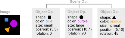
Figure 5: Setup for the oracle representation used to compute TRE. The “Object” operator is a small neural network over the features of the object. The “Scene” operator is a deterministic average.

We initialize a vector embedding for each possible color, shape, size, x coordinate, and y coordinate. Then, we define two compositional operators: first, the “Object” operator ingests the vectorized color, shape, size, and position and returns a single “Object” vector. We parameterize the “Object” operator as a MLP of varying depth. ((Andreas, 2019) assumed fixed composition by averaging, which corresponds to the special case where the “Object” MLP is linear.) Second, the “Scene” operator averages a set of “Object” vectors into a “Scene” vector. See Fig. 5 for an example. The primitive embeddings and the parameters of the “Object” operator are optimized with SGD using the distance between our image representation and the corresponding “Scene” vector as an objective. We experiment with L₁ and L₂ distance. Constructing the oracle representation in this manner ensures an object-oriented representation. Thus, we can treat the TRE score with respect to the variational image representation as a measure of its abstraction.

Table 4 measures how well VAEVAE and VAEGAN image representations can be reconstructed from the oracle representation. Compared to unimodal baselines, our model family has consistently lower TRE scores. This indicates that the representations learned mutimodally better reflect the underlying object features of this domain, abstracting away from the lower level visual information. Also, VAEGAN consistently outperforms VAEVAE, which suggests that a stronger visual model is important for capturing compositionality. As we vary the expressivity of the “Object” MLP from purely linear to three layers with ReLU, the patterns remain consistent. In the supplement Sec. E, we explore a weaker version of TRE where we use a bag-of-words feature set to represent language (e.g. color of triangles, number of triangles, color of squares, etc) with summation as the composition operator, as done in (Andreas, 2019). We find similar patterns to Table 4.

Model	Oracle	TRE (L2)	TRE (L1)
VAE	Linear	$4.468\pm 0.011$	$21.489\pm 0.058$
GAN+ALI	Linear	$4.606\pm 0.011$	$19.507\pm 0.051$
VAEVAE	Linear	$3.686\pm 0.009$	$16.188\pm 0.046$
VAEGAN	Linear	$\mathbf{2.049\pm 0.008}$	$\mathbf{10.387\pm 0.043}$
VAE	2-MLP	$2.806\pm 0.008$	$13.776\pm 0.042$
GAN+ALI	2-MLP	$2.397\pm 0.008$	$11.099\pm 0.033$
VAEVAE	2-MLP	$1.955\pm 0.008$	$10.355\pm 0.035$
VAEGAN	2-MLP	$\mathbf{1.874\pm 0.007}$	$\mathbf{9.595\pm 0.037}$
VAE	3-MLP	$2.605\pm 0.008$	$12.688\pm 0.039$
GAN+ALI	3-MLP	$2.239\pm 0.007$	$10.535\pm 0.033$
VAEVAE	3-MLP	$1.835\pm 0.008$	$8.743\pm 0.031$
VAEGAN	3-MLP	$\mathbf{1.617\pm 0.006}$	$\mathbf{8.212\pm 0.029}$

Table 4: Measuring compositionality on image representations $q_{\phi}({\bm{z}}|{\bm{x}})$ using the TRE metric and the MiniShapeWorld dataset: a lower number is better. Image features learned using VAEVAE and VAEGAN models report better TRE scores.

8.2 Object Detection

In addition to measuring compositionality directly, we can infer the impact of language on visual representations through transfer tasks that require knowledge of objects, relations, and attributes. Here, we consider bounding box prediction. The hypothesis is that image representations learned in a multimodal setting should contain more information about objects, since language aptly describes the objects in a scene. This should make it easier to identify the locations of objects in an image.

To test this hypothesis, we first take the COCO 2017 (Chen et al., 2015) dataset and pretrain a multimodal generative model e.g. VAEVAE or VAEGAN. Next, we train a well-known single-shot detection model, YOLOv3 (Redmon and Farhadi, 2018; Redmon et al., 2016) with the following edit: using a linear layer we expand the multimodal embedding to be $(1,S,S)$ where $S$ is the maximum input size at the current YOLO layer. Since it is common to train YOLOv3 with multiscale inputs, we use an adaptive pooling layer to reshape the embedding to be $(1,S_{\text{cur}},S_{\text{cur}})$ where $S_{\text{cur}}$ is the size of the inputs in the current minibatch and layer. At each residual block with input of shape $(F,S_{\text{cur}},S_{\text{cur}})$, we append the multimodal filter followed by a 1x1 convolution to project the input back to $F$ filters. Since there are several residual blocks in the YOLOv3 model, the intuition of the design to repeatedly offer information from the multimodal embedding to the detection model. The parameters of the generative model are frozen so training YOLO does not change the multimodal representation. We train for 500k iterations and measure AP[IoU=0.5] and AP[IoU=0.5:0.95] every 5000 iterations on the test set.

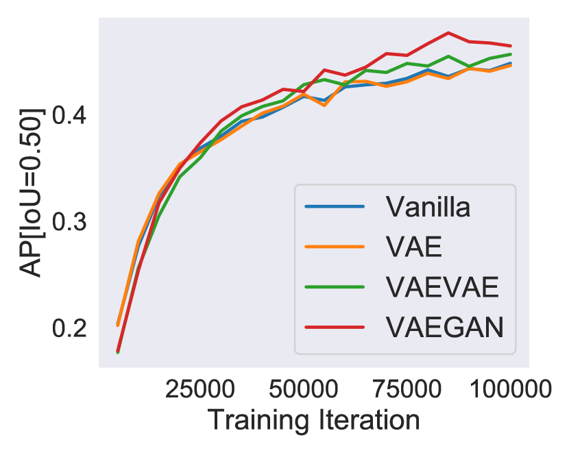
(a)

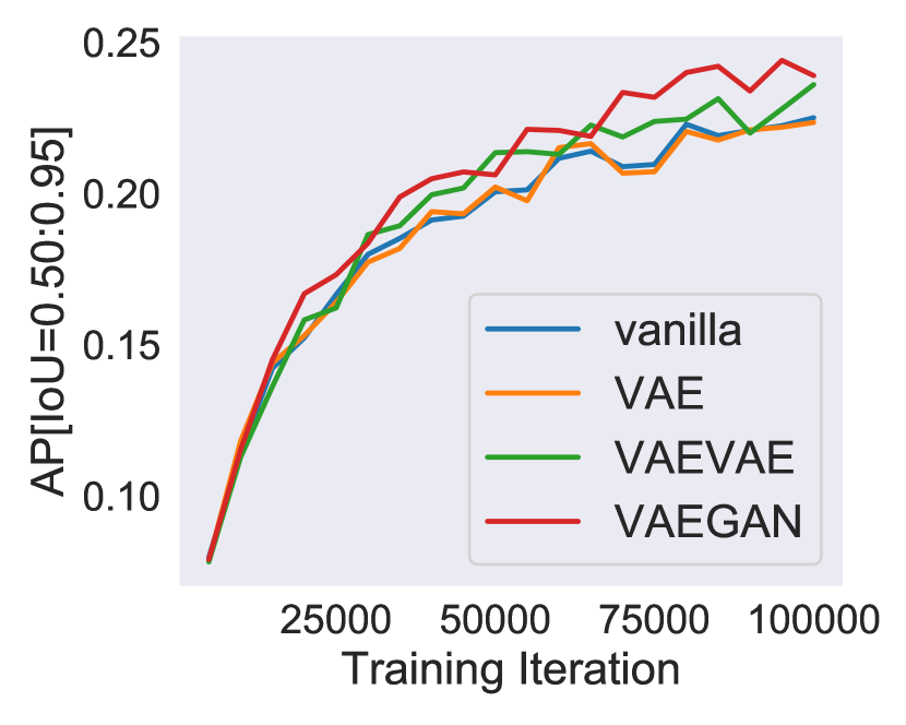
(b)

Figure 6: Comparison of trajectories showing average precisions measured every 5000 training iterations. Adding VAEVAE and VAEGAN image embeddings from $q({\bm{z}}|{\bm{x}})$ (note that no language is explicitly given) to the YOLOv3 model improves learning speed, reaching higher evaluation metrics earlier in training.

In Fig. 6, we find YOLOv3 with “multimodal” image features learns faster, evidenced by the red (VAEGAN) and green (VAEVAE) curves bounding the blue (standard) one from above. Besides the vanilla YOLOv3, we also include a baseline using image representations learned without language, from a VAE. Notably, the plots show that this baseline was almost identical in training trajectory to the vanilla YOLOv3 model, which is sensible since YOLOv3 already includes pretrained Darknet image features. Since DarkNet53 is a much larger model than the VAE, we do not expect the VAE image features do not offer any additional information. These results are encouraging, as they suggest that multimodal features can help us learn to perform complex visual tasks more efficiently. In many ways, language describing an image acts as strong supervision signal for any task involving the objects and relations in the image. Rather than initializing our bounding box detection models from image features alone (which may be less compositional), we find that we need fewer epochs or fewer parameters by using a multimodal initialization. For large models like YOLOv3 which take significant computation, faster learning can make a large impact.

	Scene Graph Det.			Scene Graph Cls.			Predicate Cls.
Recall at	20	50	100	20	50	100	20	50	100
LSVRD (Zhang et al., 2019b)	12.5	18.5	23.3	22.8	23.2	23.2	45.7	46.5	46.5
LSVRD + VAE	12.4	18.3	23.0	22.9	23.3	23.3	45.7	46.6	46.6
LSVRD + VAEGAN	12.5	18.5	23.4	33.1	33.9	33.9	55.0	56.1	56.2
LSVRD + Word2Vec (Zhang et al., 2019b)	20.2	27.4	32.1	36.2	36.9	36.9	67.4	69.0	69.0
LSVRD + VAE + Word2Vec	20.2	27.1	32.0	36.0	36.7	36.7	67.5	68.8	68.8
LSVRD + VAEGAN + Word2Vec	20.2	27.3	32.2	36.7	37.2	37.2	67.9	69.3	69.3

Table 5: Comparison with one of the state-of-the-art visual relation models on the VG200 dataset. In particular, we measure the effect of VAEGAN image representations (trained in a multimodal setting) on the “Large Scale VRD” architecture.

8.3 Visual Relation Prediction

The second transfer task we consider is relation prediction (e.g. is the person driving the car?), of which a sub-task is object detection. Since we have shown promising results with predicting bounding boxes, we might hope that language describing objects and relations in an image can have a similar effect here.

We use the Visual Genome dataset (Krishna et al., 2017), which contains images with annotated object labels, bounding boxes, and captions describing the objects in the scene. We first train the VAEVAE or VAEGAN on the image and captions alone, after which we only keep the image encoder, $q_{\phi}({\bm{z}}|{\bm{x}})$ to extract representations. For relation prediction, we use a popular subset of Visual Genome called VG200 Xu et al. (2017); Newell and Deng (2017); Zellers et al. (2018); Yang et al. (2018); Zhang et al. (2019b). VG200 contains 150 object categories and 50 predicate categories.

We pick a state-of-the-art relation predictor built on the MaskRCNN architecture He et al. (2017), denoted LSVRD (Zhang et al., 2019a) and edit the architecture to include the multimodal embedding. The LSVRD architecture contains two RCNN components, whose outputs are fed into the different heads for classification, detection, and relation prediction. For each RCNN, we combine the output of its base convolutional body (call this $a$) with the multimodal embedding in a similar fashion as above: assuming $a$ has $F$ filters, the embedding is resized to a single filter of matching width and height to $a$ (this is done via adaptive pooling to handle multiscale inputs). Then, concatenating the multimodal filter with $a$ for a total of $F+1$ filters, we use a 1x1 convolutional layer to output $F$ filters. The rest of the LSVRD network is untouched. As in (Zhang et al., 2019a), during training, the true bounding box and object classes are given to the model. For evaluation, Zhang et al. compute three metrics: scene graph detection (SGDET) where neither the bounding box nor the object class is given, scene graph classifcation (SGCLS) where only the bounding box is given, and predicate classification (PRDCLS) where both are given.

Zhang et al. already explores directly adding language features by embedding the object and predicate names with Word2Vec (Mikolov et al., 2013), which we find in Table 5 to significantly improve performance. Word2vec provides a good prior over which relations are semantically plausible, which is especially important given the sparse labels in VG200. We compare LSVRD with and without Word2vec to LSVRD with multimodal embeddings, the latter of which we expect to provide compositional image features that may positively impact learning.

Table 5 show results for six variations of LSVRD. First, we were able to reproduce the improvements in performance from using Word2Vec embeddings. Second, we point out that adding VAE embeddings to LSVRD did not impact performance – since LSVRD uses a pretrained object detection model that captures most of the salient visual features already. However, adding VAEGAN image features trained with the presence of natural language leads to significant improvements in SGCLS and PRDCLS (around 10% without Word2Vec). Critically, no explicit language features are given, the VAEGAN features are from the image encoder alone. Despite that, the performance of LSVRD + VAEGAN close the gap to using pre-trained Word2Vec embeddings. Given the previous evidence of compositionality in our multimodal representations, we suspect the VAEGAN image fatures to contain information describing objects and relations in an image imbued by language during pre-training. Finally, we separately train a version of LSVRD with both Word2Vec and VAEGAN representations. Since VAEGAN representations were exposed to complete sentences rather than individual words, we might expect further improvements. The last row of Table 5 shows a modest but consistent 0.3 to 0.5 percent increase in SGCLS and PRDCLS over a SOTA visual relation model.

9 Related Work

In recent years, there has been a series of multimodal deep generative models. We provide an overview of a few below.

Conditional Models

Many of the earlier multimodal generative models focus on conditional distributions. For example, given two modalities ${\bm{x}}$ and ${\bm{y}}$, conditional VAEs (CVAE) (Sohn et al., 2015) lower bound $\log p_{\theta}({\bm{x}}|{\bm{y}})$ where ${\bm{y}}$ is often labels (Radford et al., 2015), attributes (Yan et al., 2016), text (Reed et al., 2016), or another image (Isola et al., 2017). Similarly, conditional GANs (CGAN) (Mirza and Osindero, 2014) facilitate sample generation conditioned on another modality. This family of models are not truly multimodal as they are not bi-directional and avoid capturing marginal and joint distributions.

Joint Models

Many of the generative models over two modalities share the same graphical model, yet differ in the objective. First, the bidirectional variational canonical correlation analysis (BiVCCA) (Wang et al., 2016) optimizes a linear combination of ELBOs using the two unimodal variational posteriors:

$$\mathcal{L}_{\text{BiVCCA}} =\mathbb{E}_{p_{d}({\bm{x}},{\bm{y}})}\left(\omega\mathbb{E}_{q_{\phi}({\bm{z}}|{\bm{x}})}\left[\log\frac{p_{\theta}({\bm{x}},{\bm{y}},{\bm{z}})}{q_{\phi}({\bm{z}}|{\bm{x}})}\right]+(1-\omega)\mathbb{E}_{q_{\phi}({\bm{z}}|{\bm{y}})}\left[\log\frac{p_{\theta}({\bm{x}},{\bm{y}},{\bm{z}})}{q_{\phi}({\bm{z}}|{\bm{y}})}\right]\right)$$

where $\omega\in[0,1]$ is a weight. In particular, this model allows for bi-directional translation between modalities. However, it avoids specifying a joint variational posterior, which places a lot of the burden to do good inference on unimodal posteriors, which is difficult for very distinct modalities.

Variations on multimodal VAEs (MVAE) (Vedantam et al., 2017; Wu and Goodman, 2018) do include a multimodal variational posterior, $q_{\phi}({\bm{z}}|{\bm{x}},{\bm{y}})$. For example, (Wu and Goodman, 2018) optimize a sum of three lower bounds:

$$\mathcal{L}_{\text{MVAE}} =\text{ELBO}_{\phi,\theta}({\bm{x}},{\bm{y}})+\text{ELBO}_{\phi,\theta}({\bm{x}})+\text{ELBO}_{\phi,\theta}({\bm{y}})$$

$$\leq\log p_{\theta}({\bm{x}},{\bm{y}})+\log p_{\theta}({\bm{x}})+\log p_{\theta}({\bm{y}})$$

where the unimodal ELBOs require unimodal posteriors: $q_{\phi}({\bm{z}}|{\bm{x}})$ and $q_{\phi}({\bm{z}}|{\bm{y}})$. Specifically, (Wu and Goodman, 2018) define the $q_{\phi}({\bm{z}}|{\bm{x}},{\bm{y}})$ as the product of the unimodal posteriors.

$$q_{\phi}({\bm{z}}|{\bm{x}},{\bm{y}})\propto q_{\phi}({\bm{z}}|{\bm{x}})q_{\phi}({\bm{z}}|{\bm{y}})p({\bm{z}})$$

assuming $q_{\phi}({\bm{z}}|\cdot)$ specifies a Gaussian distribution and a product of Gaussians is itself Gaussian. While this is an elegant formulation, we note that $\mathcal{L}_{\text{MVAE}}$ double counts the marginal distributions.

$$\mathcal{L}_{\text{MVAE}} \leq 2\log p_{\theta}({\bm{x}})+\log p_{\theta}({\bm{y}})+\log p_{\theta}({\bm{y}}|{\bm{x}})$$

$$=\log p_{\theta}({\bm{x}})+2\log p_{\theta}({\bm{y}})+\log p_{\theta}({\bm{x}}|{\bm{y}})$$

This could have undesirable consequences in prioritizing the marginals over the conditionals, leading to poor cross-modality sampling. Finally, another similar model is the joint multimodal VAE (JMVAE) (Suzuki et al., 2016), which optimizes:

$$\mathcal{L}_{\text{JMVAE}} =\mathbb{E}_{p_{d}({\bm{x}},{\bm{y}})}\left[\text{ELBO}_{\phi,\theta}({\bm{x}},{\bm{y}})-\omega D_{\mathrm{KL}}(q_{\phi}({\bm{z}}|{\bm{x}},{\bm{y}})||q_{\phi}({\bm{z}}|{\bm{x}}))-\omega D_{\mathrm{KL}}(q_{\phi}({\bm{z}}|{\bm{x}},{\bm{y}})||q_{\phi}({\bm{z}}|{\bm{y}}))\right]$$

where $\omega\in\mathbb{R}^{+}$ is a hyperparameter. Critically, this is very similar to the two conditional divergence terms in our multimodal objective, $\mathcal{L}_{\text{M}}$. In (Suzuki et al., 2016), the authors have a similar derivation to Lemma 1 that shows that the JMVAE is bounded:

$$\mathcal{L}_{\text{JMVAE}}\leq\log p_{\theta}({\bm{x}}|{\bm{y}})+\log p_{\theta}({\bm{y}}|{\bm{x}})$$

Almost opposite to the MVAEs, the JMVAE prioritizes the conditionals over the marginals. Further, it does not faithfully lower bound the joint probability, $\log p_{\theta}({\bm{x}},{\bm{y}})$.

Our class of generative models neither over-prioritizes the marginals or conditionals and forms a valid lower bound on the joint density, $\log p_{\theta}({\bm{x}},{\bm{y}})$. Rather than an ad-hoc solution to missing modalities, we formally motivate the KL divergence between the joint and unimodal variational posteriors by decomposing the joint variational divergence into a marginal and conditional term. Lastly, our class of models is able to extend to likelihood-free models, which proved useful in realistic settings.

Hybrid Models

A number of models combine VAEs with GANs and Flows in the unimodal setting. Larsen et al. (2015) share parameters between the GAN generator and VAE decoder to learn more robust feature representations. Edupuganti et al. (2019) use a similar model to generate crisp images of MRI images. Wan et al. (2017) train a VAE and GAN (with ALI) on a bimodal task of reconstructing hand poses and depth images with a learned mapping between the VAE and GAN latent spaces. On the other hand, VAEs and flows have been combined (in the unimodal setting) to transform the variational posterior to a more complex family of distributions. Rezende and Mohamed (2015); Tomczak and Welling (2016); Kingma et al. (2016) apply a series of $k$ invertible transformations to $z\sim q_{\phi}(z|x)$ such that $f_{\theta}^{k}(z)$ is distributed to more expressive distribution, leading to better density estimation and sample quality. To the best of our knowledge, our class of models is the first to combine VAEs, GANs, and flow models in the multimodal setting. Further, applying such models to discrete and continuous modalities, especially images and text, is novel.

10 Conclusion

In this paper we introduced an objective for training a family of multimodal generative models. We performed a series of experiments measuring performance on marginal density estimation and translation between modalities. We found appealing results across a set of multimodal domains, including many datasets with images and text which has not been explored before in the generative setting. In particular, we found that combining different generative families like VAEs and GANs led to strong multimodal results. Finally, we conducted a thorough analysis of the effects of missing data and weak supervision on multimodal learning. We found the proposed VAEVAE and VAEGAN to outperform other generative models under high levels of missing data. Moreover, latent features learned from image distributions under the presence of language capture a notion of compositionality that led to better performance in downstream tasks. Future work could investigate applying these ideas to modelling video (Tan et al., 2019), where each frame contains visual, audio, and textual information.

A Datasets and Hyperparameters

For all experiments in Sec. 4, 5, we resized images to be 32 by 32 (note: this is different than the usual setup for MNIST, which uses 28 by 28). During training, we use 40 latent dimensions, a batch size of 64, and the Adam optimizer (Kingma and Ba, 2014). We train all models for 200 epochs. For GAN models we take the parameters from the last epoch; for all others, we take the epoch with the highest test objective as measured on the validation set. For VAE and NVP models we use a learning rate of 2e-4; for GAN models we use 2e-4 for the generator and 1e-5 for the discriminator. We found this to be important to help fight modal collapse. For grayscale and color images, we parameterize $p({\bm{x}}|{\bm{z}})$ with a Bernoulli likelihood. For labels, we use a Bernoulli likelihood for CelebA and a Categorical likelihood otherwise For text, we again use a Categorical likelihood over all words in each sentence.

MNIST

We use the MNIST hand-written digits (numbers 0 through 9) dataset (LeCun et al., 1998) with 50,000 examples for training, 10,000 validation, 10,000 testing.

FashionMNIST

This is an MNIST-like fashion dataset containing grayscale images of clothing from 10 classes—skirts, shoes, t-shirts, etc Xiao et al. (2017). This is intended to be more difficult visually than MNIST. We use the same data splits as MNIST.

CIFAR10

The CIFAR10 dataset contains 60,000 color images of ten classes (e.g. airplane, dog, ship). We use the same data splits as MNIST. Images in CIFAR10 contain much richer content than MNIST and FashionMNIST. As such, VAEs are known to struggle with sample quality, often generating very blurry images (as evidenced in this paper among many).

CelebA

The CelebFaces and Attributes (CelebA) dataset (Liu et al., 2015) contains over 200k images of celebrities. Each image is tagged with 40 attributes i.e. wears glasses, or has bangs. We use the aligned and cropped version with a selected 18 visually distinctive (and balanced) attributes, as done in (Perarnau et al., 2016).

MNIST Math

Using MNIST, we build an image-captioning dataset using arithmetic expressions that evaluate to a digit between 0 and 9 inclusive. To build a math equation, we sample a number of “+” operators (call this $k$) between 1 and 5 uniformly. Then we randomly sample $k+1$ operands (digits between 0 and 9). Following this, we rejection sample, throwing away equations that evaluate to greater than 9. Finally, we can randomly match an image in MNIST with an equation that evaluates to its corresponding label. Training and testing splits are kept as in the original MNIST.

Chairs In Context

The Chairs in Context (CIC) dataset contains 78,789 utterances, each produced by a human in conversation with another human. Specifically, this data was collected using a reference game: two participants use an online web environment where every trial, participant A is given 3 images of chairs and tasked to describe a target chair to participant B, who apriori does not know which chair is being described. In total, there are 4,511 unique chair renderings, taken from ShapeNet. In their work (Achlioptas et al., 2018), the authors focus on investigating the varying contexts (the two chairs that were not chosen) on the utterance produced. Here, we ignore context completely, taking only the target chair image and the corresponding utterance.

Flickr30k

The Flickr30k dataset is a standard benchmark dataset for image captioning, containing 158k captions generated from query text used in image search (on Flickr) for 30k images. Multiple captions are used for each image. We treat each instance as an independent observation. Each caption tends to only describe one or two of the subjects (among many) in the scene.

COCO Captions

The Microsoft COCO (Lin et al., 2014) dataset contains images of complex everyday scenes of common objects in natural contexts. In total there are 328k images, each with 5 captions describing a subset of objects in the scene. Given the already large size of the dataset, we only use the first caption for each image.

B Evaluation

For image and label datasets, we measure the image marginal and joint log likelihoods:

$$\mathbb{E}_{p_{d}^{\text{test}}({\bm{x}})}[\log p_{\theta}({\bm{x}})] =\mathbb{E}_{p_{d}^{\text{test}}({\bm{x}})}[\log\mathbb{E}_{q_{\phi}({\bm{z}}|{\bm{x}})}[\frac{p_{\theta}({\bm{x}}|{\bm{z}})p({\bm{z}})}{q_{\phi}({\bm{z}}|{\bm{x}})}]]$$

$$\mathbb{E}_{p_{d}^{\text{test}}({\bm{x}},{\bm{y}})}[\log p_{\theta}({\bm{x}},{\bm{y}})] =\mathbb{E}_{p_{d}^{\text{test}}({\bm{x}},{\bm{y}})}[\log\mathbb{E}_{q_{\phi}({\bm{z}}|{\bm{x}},{\bm{y}})}[\frac{p_{\theta}({\bm{x}}|{\bm{z}})p_{\theta}({\bm{y}}|{\bm{z}})p({\bm{z}})}{q_{\phi}({\bm{z}}|{\bm{x}},{\bm{y}})}]]$$

where the superscript test indicates an empirical distribution not seen in training. In addition, for image and text datasets, we measure the text marginal log likelihood by:

$$\mathbb{E}_{p_{d}^{\text{test}}({\bm{y}})}[\log p_{\theta}({\bm{y}})]=\mathbb{E}_{p_{d}^{\text{test}}({\bm{y}})}[\log\mathbb{E}_{q_{\phi}({\bm{z}}|{\bm{y}})}[\frac{p({\bm{z}})\prod_{{\bm{w}}_{i}\in{\bm{y}}}p_{\theta}({\bm{w}}_{i}|{\bm{z}},\vec{{\bm{w}}}_{-i})}{q_{\phi}({\bm{z}}|{\bm{y}})}]]$$ (33)

where an utterance is made up of a sequence of words $y=({\bm{w}}_{1},{\bm{w}}_{2},...)$ and $\vec{{\bm{w}}}_{-i}=({\bm{w}}_{1},...,{\bm{w}}_{i-1})$ represent the words up to index $i$. In replacement of classification error, we compute conditional perplexity:

$$\text{perp}=\exp\{-\frac{1}{N^{\text{test}}}\sum_{j=1}^{N^{\text{test}}}\frac{1}{|y_{j}|}\sum_{w_{i}\in{\bm{y}}_{j}}\log p_{\theta}({\bm{w}}_{i}|{\bm{z}},\vec{{\bm{w}}}_{-i})\}$$ (34)

where ${\bm{z}}\sim q_{\phi}({\bm{z}}|{\bm{y}})$ and $N^{\text{test}}$ is the size of the test set.

C Model Architectures

We discuss a few choices for model architectures. Exact implementations will be available online. In choosing these, we prioritized quick training times and relevant designs from previous literature. Future work can explore more complex architectures and greater hyperparameter tuning. For all models, we use ReLU or LeakyReLU. For all image generative networks (in VAEs and GANs) we use a sequence of 3 to 4 de-convolutional layers followed by a convolutional layer and fully connected units. For all image inference networks, we use 3 to 4 convolutional layers. GAN discriminators are similarly designed. GAN models additionally have batch normalization after each convolutional layers (as in DCGAN). Encoding and Decoding networks for labels have 3 linear layers given that this modality is very simple. For all text based networks, we use RNNVAE style encoders and decoders (Bowman et al., 2015); in this context, word dropout is extremely important to discourage ignoring the latent variable in this autoregressive model. For flow based models, we use the realNVP design (Dinh et al., 2016) with ResNets (He et al., 2016) in each coupling layer.

D Training with Unpaired Data

As referenced by the main text, Alg. 1 shows how to train a multimodal generative model with unpaired data. In short, sample unimodal data to compute the “unimodal” terms in the objective. The same algorithm can be used for VAEVAE and VAEGAN models.

Algorithm 1 Forward Pass with Unpaired Data

  Input: Supervision example $({\bm{x}},{\bm{y}})$, Unsupervised example ${\bm{x}}^{\prime}$, Unsupervised example ${\bm{y}}^{\prime}$

  ${\bm{z}}^{\prime},{\bm{z}}_{{\bm{x}}},{\bm{z}}_{{\bm{y}}}=q_{\phi}({\bm{z}}|{\bm{x}},{\bm{y}}),q_{\phi}({\bm{z}}|{\bm{x}}),q_{\phi}({\bm{z}}|{\bm{y}})$

  $d_{1}=D(q_{\phi}({\bm{z}}^{\prime}|{\bm{x}},{\bm{y}})||q_{\phi}({\bm{z}}^{\prime}|{\bm{y}}))$

  $d_{2}=D(q_{\phi}({\bm{z}}^{\prime}|{\bm{x}},{\bm{y}})||q_{\phi}({\bm{z}}^{\prime}|{\bm{x}}))$

  $\mathcal{L}^{\prime}=\log p_{\theta}({\bm{x}}|{\bm{z}}^{\prime})+\log p_{\theta}({\bm{y}}|{\bm{z}}^{\prime})+d_{1}+d_{2}$

  $\mathcal{L}_{\bm{x}}=\log p_{\theta}({\bm{x}}^{\prime}|{\bm{z}}_{\bm{x}})+D(q_{\phi}({\bm{z}}_{\bm{x}}|{\bm{x}}^{\prime})||p({\bm{z}}))$

  $\mathcal{L}_{\bm{y}}=\log p_{\theta}({\bm{y}}^{\prime}|{\bm{z}}_{\bm{y}})+D(q_{\phi}({\bm{z}}_{\bm{y}}|{\bm{y}}^{\prime})||p({\bm{z}}))$

  $\mathcal{L}_{\text{WS}}=\mathcal{L}^{\prime}+\mathcal{L}_{\bm{x}}+\mathcal{L}_{\bm{y}}$

E Additional Compositionality Results

In the main text, we used an elaborate procedure to define the oracle representation with the goal being a representation that identifies each individual object in the image. In their original work, (Andreas, 2019) suggested a much simpler framework: Define the vector embeddings as a bag-of-word features from the caption (e.g. there is a blue square and a red triangle) of a ShapeWorld image and sum over them as the composition operator. While straightforward, we found this setup lacked the information to identify individual objects. Critically, these features did not include the size, rotation, and location of objects. Because these features were missing, the bag-of-words could not distinguish between multiple red triangle in image, for example. However, to stay consistent to prior work, we also include results in Table. 6 of TRE as presented in (Andreas, 2019).

Model	TRE (L2)	TRE (L1)
VAE	$7.523\pm 0.034$	$81.128\pm 0.396$
GAN+ALI	$7.513\pm 0.031$	$80.910\pm 0.358$
VAEVAE	$5.953\pm 0.033$	$68.287\pm 0.346$
VAEGAN	$\mathbf{2.304\pm 0.026}$	$26.382\pm 0.362$
VAEGAN§	$3.431\pm 0.021$	$\mathbf{14.416\pm 0.104}$

Table 6: Estimating compositionality with TRE score as computed in (Andreas, 2019).

F Sample Zoo

Fig. 7, 8 show randomly chosen samples for VAEVAE, VAEGAN, and VAENVP models on a suite of multimodal datasets. For those involving images and text, we show generated captions as well.

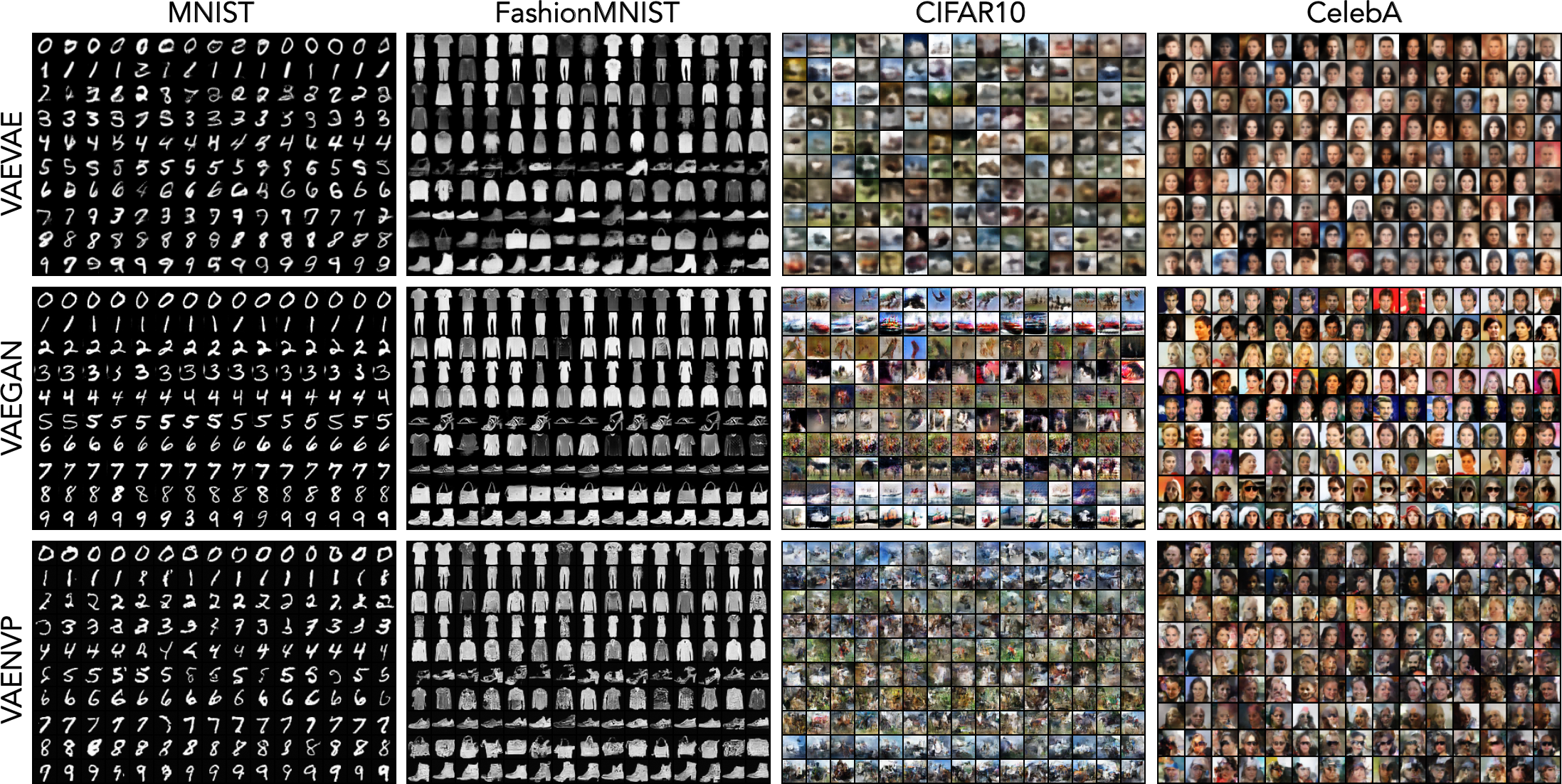
Figure 7: Image and Label Sample Zoo – Samples generated by VAEVAE, VAEGAN, and VAENVP models. Each row contains samples of the same label (e.g. digit number for MNIST or attribute in CelebA). VAEVAE models struggle with blurriness for richer images.

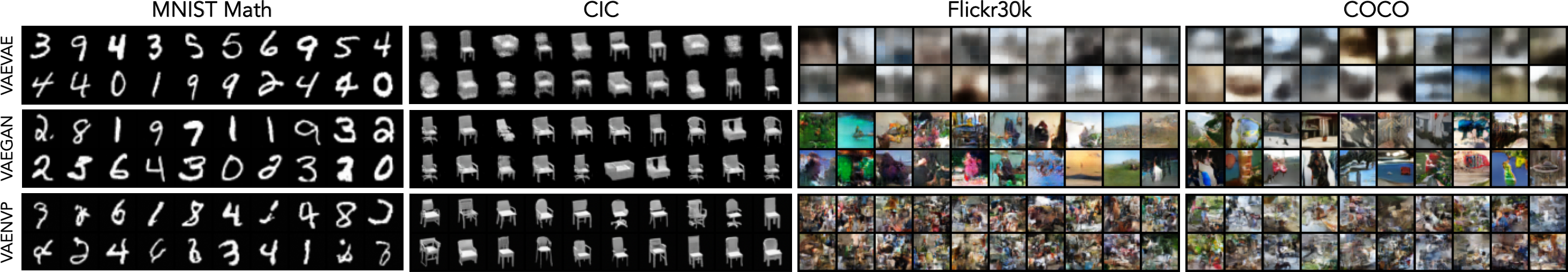
(a) Marginal Samples

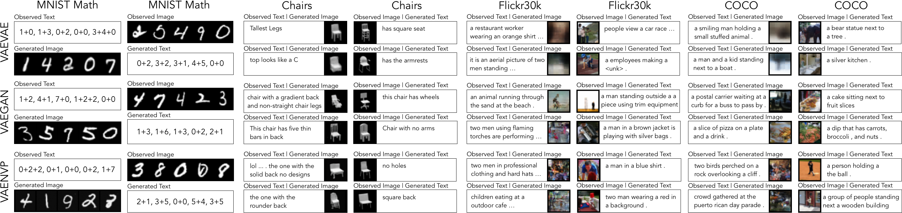
(b) Conditional Samples

Figure 8: Image and Text Sample Zoo – Marginal samples and conditional samples generated by VAEVAE, VAEGAN, and VAENVP models. VAEGAN significantly outperforms other models in sample quality for more complex image domains.

G Details on Downstream Image Experiments

Object Detection

When training VAEVAE or VAEGAN, we use 100 latent dimensions and reshape images to be a fixed 64 by 64 pixel size. As in previous experiments, we use a learning rate of 2e-4 and train for 200 epochs with a batch size of 64 and the Adam optimizer. We use an RNNVAE for the text generative model and a convolutional network for the image generative model. These are the same as describe in Sec. C.

Visual Relation Detection

Because the images in Visual Genome are in general more complex, we use 256 latent dimensions and reshape images to be 64 by 64 pixels. All other choices are as in object detection.

H Using Representations in Reference Games

In this section of the Appendix, we investigate a possible use case of multimodal representations in grounded language learning (not presented in the main text). Future work could explore this direction in more detail.

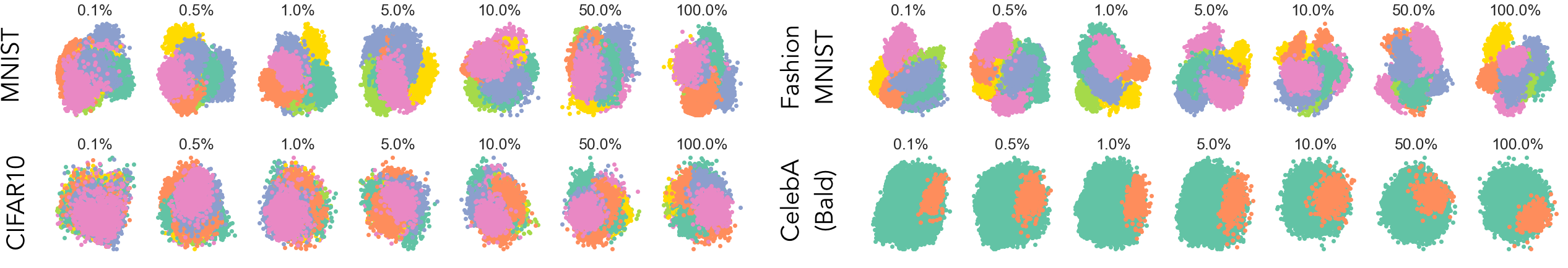
Figure 9: PCA projections of VAEVAE (joint) embeddings for varying levels of supervision across four image and label datasets. Increased supervision tends towards more well defined clusters.

One of the attractive properties of a generative model is a learned (latent) representation for a given image. Likewise, we can obtain a joint representation using a multimodal generative model. Specifically, we take the mean of the variational posterior $q_{\phi}(z|x,y)$ as a “joint” encoding of $x$ and $y$. For instance, Fig. 9 shows a 2-dimensional PCA projection of embeddings from the test set of four labelled image datasets as the amount of supervision is varied from low (0.1%) to high (100%). We note that the separation between classes increases (more defined clusters) as supervision increases. In particular, even with 5% supervision (lower for simpler decision boundaries), we start to see distinct clusters form, suggesting that we can efficiently compress the underlying structure of the data domain without over-dependence on supervision. These embeddings may be useful for downstream predictive tasks. We find similar behavior for VAEGAN models.

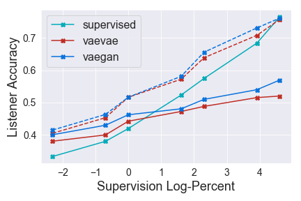
(a)

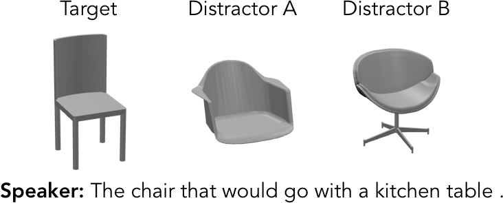
(b)

Figure 10: (a) Weak supervision experiment for listeners in a Chairs reference game. (b) Example of a target chair (chosen by listener), two distractor chairs, and a speaker utterance.

One of the attractive properties of our generative model is a multimodal representation that may be used for downstream tasks. For example, we can apply the learned representation to reference games (Achlioptas et al., 2019; Cohn-Gordon et al., 2018; Hawkins et al., 2017) as used in computational cognitive science. Reference games are an experiment tool for studying human pragmatic reasoning in a controlled setting: there are two agents: a listener and a speaker. Given a context of 3 possible images, the speaker’s task is to describe one of them. The listener’s role is to guess the speaker’s intended referent from the set of three. A large branch of research studies how to model the listener and speaker as Bayesian computational models (Goodman and Frank, 2016). More recent work (Cohn-Gordon et al., 2018) has instead parameterized the listener and speaker as deep neural networks. Within reference games, paired data is collected by human agents using Mechanical Turk, meaning that common dataset sizes are limited to a few thousand at best. This is not enough to train many deep models and therefore, a perfect use case for weakly supervised learning.

Here, we begin to study applying multimodal generative models to model listener behavior. To gauge performance, we measure how well a computational model can choose the “correct” image out of three given a speaker utterance as compared to human listener choices. In particular, the Chairs in Context (CIC) dataset was released as a reference game dataset. In our experiments above, we only used the utterance and target image but the full dataset contains a speaker utterance, a set of three chair images, and the (“target”) chair chosen by a listener. We only consider set of images in the far context, meaning the three chairs have visually distinctive features. Future work should explore the more difficult close context. In Fig. 10, we compare the accuracy of a supervised neural model as used in reference game literature (trained specifically for the reference game task) and a VAEVAE and VAEGAN as we vary the amount of paired data. With full supervision, the dataset contains 67k examples. To make a prediction for which chair the speaker is referencing using a generative model, we take $\arg\max_{i\in\{1,2,3\}}p_{\theta}({\bm{x}}={\bm{x}}_{i}|{\bm{z}}=\mathbf{\mu})$ where $\mathbf{\mu}$ is the mean for posterior $q_{\phi}({\bm{z}}|{\bm{y}})$. The set $\{{\bm{x}}_{1},{\bm{x}}_{2},{\bm{x}}_{3}\}$ represents the images in context and ${\bm{y}}$ represents the speaker utterance. Fig. 10 shows that a VAEVAE and VAEGAN outperform a supervised model in the low data regime (around 100 to 1000 examples). Beyond 1000 examples, supervised networks specifically trained as listeners in a reference game out-perform the generative models. In some sense, it is not fair to compare these generative models and the supervised model since only the latter was trained with knowledge of the reference game setup. Perhaps a more fair comparison would be to use the unsupervised embeddings learned by VAEVAE or VAEGAN and fit a small network to play the reference game. The dotted lines in Fig. 10 show exactly this; we can see the performance is much higher than the generative models alone and higher than the supervised baseline as well. Future work should investigate other reference games (Monroe et al., 2017) as well as possibility of using unpaired text and images for more efficient learning. The ability to learn listeners with less data could save time and resources for many future cognitive studies.

References

- Achlioptas et al. (2018) Panos Achlioptas, Judy E Fan, Robert XD Hawkins, Noah D Goodman, and Leo Guibas. Learning to refer to 3d objects with natural language. 2018.
- Achlioptas et al. (2019) Panos Achlioptas, Judy Fan, Robert XD Hawkins, Noah D Goodman, and Leonidas J Guibas. Shapeglot: Learning language for shape differentiation. arXiv preprint arXiv:1905.02925, 2019.
- Andreas (2019) Jacob Andreas. Measuring compositionality in representation learning. arXiv preprint arXiv:1902.07181, 2019.
- Arjovsky et al. (2017) Martin Arjovsky, Soumith Chintala, and Léon Bottou. Wasserstein gan. arXiv preprint arXiv:1701.07875, 2017.
- Baruch and Keller (2018) Elad Ben Baruch and Yosi Keller. Multimodal matching using a hybrid convolutional neural network. arXiv preprint arXiv:1810.12941, 2018.
- Bowman et al. (2015) Samuel R Bowman, Luke Vilnis, Oriol Vinyals, Andrew M Dai, Rafal Jozefowicz, and Samy Bengio. Generating sentences from a continuous space. arXiv preprint arXiv:1511.06349, 2015.
- Chang et al. (2015) Angel X Chang, Thomas Funkhouser, Leonidas Guibas, Pat Hanrahan, Qixing Huang, Zimo Li, Silvio Savarese, Manolis Savva, Shuran Song, Hao Su, et al. Shapenet: An information-rich 3d model repository. arXiv preprint arXiv:1512.03012, 2015.
- Chen et al. (2015) Xinlei Chen, Hao Fang, Tsung-Yi Lin, Ramakrishna Vedantam, Saurabh Gupta, Piotr Dollár, and C Lawrence Zitnick. Microsoft coco captions: Data collection and evaluation server. arXiv preprint arXiv:1504.00325, 2015.
- Chen et al. (2017) Yunpeng Chen, Jianan Li, Huaxin Xiao, Xiaojie Jin, Shuicheng Yan, and Jiashi Feng. Dual path networks. In Advances in Neural Information Processing Systems, pages 4467–4475, 2017.
- Cohn-Gordon et al. (2018) Reuben Cohn-Gordon, Noah Goodman, and Christopher Potts. Pragmatically informative image captioning with character-level inference. arXiv preprint arXiv:1804.05417, 2018.
- Dinh et al. (2014) Laurent Dinh, David Krueger, and Yoshua Bengio. Nice: Non-linear independent components estimation. arXiv preprint arXiv:1410.8516, 2014.
- Dinh et al. (2016) Laurent Dinh, Jascha Sohl-Dickstein, and Samy Bengio. Density estimation using real nvp. arXiv preprint arXiv:1605.08803, 2016.
- Dumoulin et al. (2016) Vincent Dumoulin, Ishmael Belghazi, Ben Poole, Olivier Mastropietro, Alex Lamb, Martin Arjovsky, and Aaron Courville. Adversarially learned inference. arXiv preprint arXiv:1606.00704, 2016.
- Edupuganti et al. (2019) Vineet Edupuganti, Morteza Mardani, Joseph Cheng, Shreyas Vasanawala, and John Pauly. Vae-gans for probabilistic compressive image recovery: Uncertainty analysis. arXiv preprint arXiv:1901.11228, 2019.
- Goodfellow et al. (2014) Ian Goodfellow, Jean Pouget-Abadie, Mehdi Mirza, Bing Xu, David Warde-Farley, Sherjil Ozair, Aaron Courville, and Yoshua Bengio. Generative adversarial nets. In Advances in neural information processing systems, pages 2672–2680, 2014.
- Goodman and Frank (2016) Noah D Goodman and Michael C Frank. Pragmatic language interpretation as probabilistic inference. Trends in cognitive sciences, 20(11):818–829, 2016.
- Grathwohl et al. (2018) Will Grathwohl, Ricky TQ Chen, Jesse Betterncourt, Ilya Sutskever, and David Duvenaud. Ffjord: Free-form continuous dynamics for scalable reversible generative models. arXiv preprint arXiv:1810.01367, 2018.
- Gulrajani et al. (2016) Ishaan Gulrajani, Kundan Kumar, Faruk Ahmed, Adrien Ali Taiga, Francesco Visin, David Vazquez, and Aaron Courville. Pixelvae: A latent variable model for natural images. arXiv preprint arXiv:1611.05013, 2016.
- Gulrajani et al. (2017) Ishaan Gulrajani, Faruk Ahmed, Martin Arjovsky, Vincent Dumoulin, and Aaron C Courville. Improved training of wasserstein gans. In Advances in Neural Information Processing Systems, pages 5767–5777, 2017.
- Hawkins et al. (2017) Robert XD Hawkins, Mike Frank, and Noah D Goodman. Convention-formation in iterated reference games. In CogSci, 2017.
- He et al. (2016) Kaiming He, Xiangyu Zhang, Shaoqing Ren, and Jian Sun. Deep residual learning for image recognition. In Proceedings of the IEEE conference on computer vision and pattern recognition, pages 770–778, 2016.
- He et al. (2017) Kaiming He, Georgia Gkioxari, Piotr Dollár, and Ross Girshick. Mask r-cnn. In Proceedings of the IEEE international conference on computer vision, pages 2961–2969, 2017.
- Hinton (1999) Geoffrey E Hinton. Products of experts. 1999.
- Huang et al. (2018) Chin-Wei Huang, David Krueger, Alexandre Lacoste, and Aaron Courville. Neural autoregressive flows. arXiv preprint arXiv:1804.00779, 2018.
- Isola et al. (2017) Phillip Isola, Jun-Yan Zhu, Tinghui Zhou, and Alexei A Efros. Image-to-image translation with conditional adversarial networks. In Proceedings of the IEEE conference on computer vision and pattern recognition, pages 1125–1134, 2017.
- Kingma and Ba (2014) Diederik P Kingma and Jimmy Ba. Adam: A method for stochastic optimization. arXiv preprint arXiv:1412.6980, 2014.
- Kingma and Welling (2013) Diederik P Kingma and Max Welling. Auto-encoding variational bayes. arXiv preprint arXiv:1312.6114, 2013.
- Kingma and Dhariwal (2018) Durk P Kingma and Prafulla Dhariwal. Glow: Generative flow with invertible 1x1 convolutions. In Advances in Neural Information Processing Systems, pages 10236–10245, 2018.
- Kingma et al. (2016) Durk P Kingma, Tim Salimans, Rafal Jozefowicz, Xi Chen, Ilya Sutskever, and Max Welling. Improved variational inference with inverse autoregressive flow. In Advances in neural information processing systems, pages 4743–4751, 2016.
- Krishna et al. (2017) Ranjay Krishna, Yuke Zhu, Oliver Groth, Justin Johnson, Kenji Hata, Joshua Kravitz, Stephanie Chen, Yannis Kalantidis, Li-Jia Li, David A Shamma, et al. Visual genome: Connecting language and vision using crowdsourced dense image annotations. International Journal of Computer Vision, 123(1):32–73, 2017.
- Kuhnle and Copestake (2017) Alexander Kuhnle and Ann Copestake. Shapeworld-a new test methodology for multimodal language understanding. arXiv preprint arXiv:1704.04517, 2017.
- Larsen et al. (2015) Anders Boesen Lindbo Larsen, Søren Kaae Sønderby, Hugo Larochelle, and Ole Winther. Autoencoding beyond pixels using a learned similarity metric. arXiv preprint arXiv:1512.09300, 2015.
- LeCun et al. (1998) Yann LeCun, Léon Bottou, Yoshua Bengio, Patrick Haffner, et al. Gradient-based learning applied to document recognition. Proceedings of the IEEE, 86(11):2278–2324, 1998.
- Lin et al. (2014) Tsung-Yi Lin, Michael Maire, Serge Belongie, James Hays, Pietro Perona, Deva Ramanan, Piotr Dollár, and C Lawrence Zitnick. Microsoft coco: Common objects in context. In European conference on computer vision, pages 740–755. Springer, 2014.
- Liu et al. (2018) Kuan Liu, Yanen Li, Ning Xu, and Prem Natarajan. Learn to combine modalities in multimodal deep learning. arXiv preprint arXiv:1805.11730, 2018.
- Liu et al. (2015) Ziwei Liu, Ping Luo, Xiaogang Wang, and Xiaoou Tang. Deep learning face attributes in the wild. In Proceedings of International Conference on Computer Vision (ICCV), 2015.
- Michel et al. (2011) Jean-Baptiste Michel, Yuan Kui Shen, Aviva Presser Aiden, Adrian Veres, Matthew K Gray, Joseph P Pickett, Dale Hoiberg, Dan Clancy, Peter Norvig, Jon Orwant, et al. Quantitative analysis of culture using millions of digitized books. science, 331(6014):176–182, 2011.
- Mikolov et al. (2013) Tomas Mikolov, Kai Chen, Greg Corrado, and Jeffrey Dean. Efficient estimation of word representations in vector space. arXiv preprint arXiv:1301.3781, 2013.
- Mirza and Osindero (2014) Mehdi Mirza and Simon Osindero. Conditional generative adversarial nets. arXiv preprint arXiv:1411.1784, 2014.
- Monroe et al. (2017) Will Monroe, Robert XD Hawkins, Noah D Goodman, and Christopher Potts. Colors in context: A pragmatic neural model for grounded language understanding. Transactions of the Association for Computational Linguistics, 5:325–338, 2017.
- Newell and Deng (2017) Alejandro Newell and Jia Deng. Pixels to graphs by associative embedding. In Advances in neural information processing systems, pages 2171–2180, 2017.
- Ngiam et al. (2011) Jiquan Ngiam, Aditya Khosla, Mingyu Kim, Juhan Nam, Honglak Lee, and Andrew Y Ng. Multimodal deep learning. In Proceedings of the 28th international conference on machine learning (ICML-11), pages 689–696, 2011.
- Nowozin et al. (2016) Sebastian Nowozin, Botond Cseke, and Ryota Tomioka. f-gan: Training generative neural samplers using variational divergence minimization. In Advances in neural information processing systems, pages 271–279, 2016.
- Papamakarios et al. (2017) George Papamakarios, Theo Pavlakou, and Iain Murray. Masked autoregressive flow for density estimation. In Advances in Neural Information Processing Systems, pages 2338–2347, 2017.
- Perarnau et al. (2016) Guim Perarnau, Joost Van De Weijer, Bogdan Raducanu, and Jose M Álvarez. Invertible conditional gans for image editing. arXiv preprint arXiv:1611.06355, 2016.
- Plummer et al. (2015) Bryan A Plummer, Liwei Wang, Chris M Cervantes, Juan C Caicedo, Julia Hockenmaier, and Svetlana Lazebnik. Flickr30k entities: Collecting region-to-phrase correspondences for richer image-to-sentence models. In Proceedings of the IEEE international conference on computer vision, pages 2641–2649, 2015.
- Radford et al. (2015) Alec Radford, Luke Metz, and Soumith Chintala. Unsupervised representation learning with deep convolutional generative adversarial networks. arXiv preprint arXiv:1511.06434, 2015.
- Redmon and Farhadi (2018) Joseph Redmon and Ali Farhadi. Yolov3: An incremental improvement. arXiv preprint arXiv:1804.02767, 2018.
- Redmon et al. (2016) Joseph Redmon, Santosh Divvala, Ross Girshick, and Ali Farhadi. You only look once: Unified, real-time object detection. In Proceedings of the IEEE conference on computer vision and pattern recognition, pages 779–788, 2016.
- Reed et al. (2016) Scott Reed, Zeynep Akata, Xinchen Yan, Lajanugen Logeswaran, Bernt Schiele, and Honglak Lee. Generative adversarial text to image synthesis. arXiv preprint arXiv:1605.05396, 2016.
- Rezende and Mohamed (2015) Danilo Jimenez Rezende and Shakir Mohamed. Variational inference with normalizing flows. arXiv preprint arXiv:1505.05770, 2015.
- Rezende et al. (2014) Danilo Jimenez Rezende, Shakir Mohamed, and Daan Wierstra. Stochastic backpropagation and approximate inference in deep generative models. arXiv preprint arXiv:1401.4082, 2014.
- Russakovsky et al. (2015) Olga Russakovsky, Jia Deng, Hao Su, Jonathan Krause, Sanjeev Satheesh, Sean Ma, Zhiheng Huang, Andrej Karpathy, Aditya Khosla, Michael Bernstein, et al. Imagenet large scale visual recognition challenge. International journal of computer vision, 115(3):211–252, 2015.
- Salimans et al. (2016) Tim Salimans, Ian Goodfellow, Wojciech Zaremba, Vicki Cheung, Alec Radford, and Xi Chen. Improved techniques for training gans. In Advances in neural information processing systems, pages 2234–2242, 2016.
- Sohn et al. (2015) Kihyuk Sohn, Honglak Lee, and Xinchen Yan. Learning structured output representation using deep conditional generative models. In Advances in neural information processing systems, pages 3483–3491, 2015.
- Suzuki et al. (2016) Masahiro Suzuki, Kotaro Nakayama, and Yutaka Matsuo. Joint multimodal learning with deep generative models. arXiv preprint arXiv:1611.01891, 2016.
- Szegedy et al. (2015) Christian Szegedy, Wei Liu, Yangqing Jia, Pierre Sermanet, Scott Reed, Dragomir Anguelov, Dumitru Erhan, Vincent Vanhoucke, and Andrew Rabinovich. Going deeper with convolutions. In Proceedings of the IEEE conference on computer vision and pattern recognition, pages 1–9, 2015.
- Tan et al. (2019) Zhi-Xuan Tan, Harold Soh, and Desmond C Ong. Factorized inference in deep markov models for incomplete multimodal time series. arXiv preprint arXiv:1905.13570, 2019.
- Tomczak and Welling (2016) Jakub M Tomczak and Max Welling. Improving variational auto-encoders using householder flow. arXiv preprint arXiv:1611.09630, 2016.
- Vedantam et al. (2017) Ramakrishna Vedantam, Ian Fischer, Jonathan Huang, and Kevin Murphy. Generative models of visually grounded imagination. arXiv preprint arXiv:1705.10762, 2017.
- Wan et al. (2017) Chengde Wan, Thomas Probst, Luc Van Gool, and Angela Yao. Crossing nets: Combining gans and vaes with a shared latent space for hand pose estimation. In Proceedings of the IEEE Conference on Computer Vision and Pattern Recognition, pages 680–689, 2017.
- Wang et al. (2016) Weiran Wang, Xinchen Yan, Honglak Lee, and Karen Livescu. Deep variational canonical correlation analysis. arXiv preprint arXiv:1610.03454, 2016.
- Wu and Goodman (2018) Mike Wu and Noah Goodman. Multimodal generative models for scalable weakly-supervised learning. In Advances in Neural Information Processing Systems, pages 5580–5590, 2018.
- Xiao et al. (2017) Han Xiao, Kashif Rasul, and Roland Vollgraf. Fashion-mnist: a novel image dataset for benchmarking machine learning algorithms. arXiv preprint arXiv:1708.07747, 2017.
- Xu et al. (2017) Danfei Xu, Yuke Zhu, Christopher B Choy, and Li Fei-Fei. Scene graph generation by iterative message passing. In Proceedings of the IEEE Conference on Computer Vision and Pattern Recognition, pages 5410–5419, 2017.
- Xu et al. (2015) Kelvin Xu, Jimmy Ba, Ryan Kiros, Kyunghyun Cho, Aaron Courville, Ruslan Salakhudinov, Rich Zemel, and Yoshua Bengio. Show, attend and tell: Neural image caption generation with visual attention. In International conference on machine learning, pages 2048–2057, 2015.
- Yan et al. (2016) Xinchen Yan, Jimei Yang, Kihyuk Sohn, and Honglak Lee. Attribute2image: Conditional image generation from visual attributes. In European Conference on Computer Vision, pages 776–791. Springer, 2016.
- Yang et al. (2018) Jianwei Yang, Jiasen Lu, Stefan Lee, Dhruv Batra, and Devi Parikh. Graph r-cnn for scene graph generation. In Proceedings of the European Conference on Computer Vision (ECCV), pages 670–685, 2018.
- Zellers et al. (2018) Rowan Zellers, Mark Yatskar, Sam Thomson, and Yejin Choi. Neural motifs: Scene graph parsing with global context. In Proceedings of the IEEE Conference on Computer Vision and Pattern Recognition, pages 5831–5840, 2018.
- Zhang et al. (2019a) Ji Zhang, Yannis Kalantidis, Marcus Rohrbach, Manohar Paluri, Ahmed Elgammal, and Mohamed Elhoseiny. Large-scale visual relationship understanding. In AAAI, 2019a.
- Zhang et al. (2019b) Ji Zhang, Yannis Kalantidis, Marcus Rohrbach, Manohar Paluri, Ahmed Elgammal, and Mohamed Elhoseiny. Large-scale visual relationship understanding. In Proceedings of the AAAI Conference on Artificial Intelligence, volume 33, pages 9185–9194, 2019b.
- Zhao et al. (2017a) Shengjia Zhao, Jiaming Song, and Stefano Ermon. Infovae: Information maximizing variational autoencoders. arXiv preprint arXiv:1706.02262, 2017a.
- Zhao et al. (2017b) Shengjia Zhao, Jiaming Song, and Stefano Ermon. Towards deeper understanding of variational autoencoding models. arXiv preprint arXiv:1702.08658, 2017b.