Efficient Querying from Weighted Binary Codes

Abstract

Binary codes are widely used to represent the data due to their small storage and efficient computation. However, there exists an ambiguity problem that lots of binary codes share the same Hamming distance to a query. To alleviate the ambiguity problem, weighted binary codes assign different weights to each bit of binary codes and compare the binary codes by the weighted Hamming distance. Till now, performing the querying from the weighted binary codes efficiently is still an open issue. In this paper, we propose a new method to rank the weighted binary codes and return the nearest weighted binary codes of the query efficiently. In our method, based on the multi-index hash tables, two algorithms, the table bucket finding algorithm and the table merging algorithm, are proposed to select the nearest weighted binary codes of the query in a non-exhaustive and accurate way. The proposed algorithms are justified by proving their theoretic properties. The experiments on three large-scale datasets validate both the search efficiency and the search accuracy of our method. Especially for the number of weighted binary codes up to one billion, our method shows a great improvement of more than 1000 times faster than the linear scan.

Introduction

With the explosive growth of data, binary codes are widely used to represent the data due to their small storage and efficient computation. Given a query, the nearest binary codes can be ranked and returned efficiently by computing the Hamming distance between the query and the binary codes. BRISK (?), ORB (?), and other binary image descriptors (?) are designed to represent the image data, and successfully used in various applications, including image matching, 3D reconstruction and object recognition. End-to-end feature learning methods (?; ?) based on the neural networks extract the binary codes from the images and are widely used in image retrieval and cross retrieval. In addition to these specific image binary codes, hashing methods (?; ?; ?; ?) are used to map different high-dimensional feature vectors into compact binary codes. Since these feature vectors may represent image data, video data, or other multimedia data, the hashing methods can be used in various multimedia retrieval applications.

However, the number of possible Hamming distance is limited and different binary codes may share the same Hamming distance to the given binary query. To alleviate this ambiguity problem and further improve the performance of binary codes, weighted binary codes are used (?; ?; ?). By assigning bitwise weights to each bit of binary codes, the distance between a pair of binary codes is calculated by weighted Hamming distance instead of Hamming distance. For example,  (?; ?) are designed to learn the weights for the binary image descriptors to improve their discriminative power for image matching. And  (?; ?) are designed to learn the weights for the binary codes generated by different hashing methods to improve their search accuracy for multimedia retrieval.

Although weighted binary codes can alleviate the ambiguity problem, querying from the binary codes by weighted Hamming distance is slower than that by Hamming distance. To accelerate the querying process from the weighted binary codes, some methods (?) use lookup tables to compute the query-independent values in advance. However, it is still an exhaustive linear scan. Some methods (?; ?) use Hamming distance to find the neighbors that have the smallest Hamming distance to the query and rank them according to the weighted Hamming distance. This non-exhaustive way is fast but cannot return the nearest weighted binary codes of the query accurately, resulting in a degraded performance of weighted binary codes in the application.

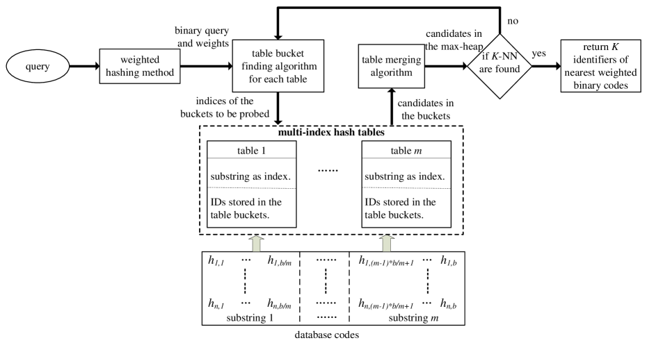
Figure 1: The diagram of our method to find the $K$ nearest weighted binary codes of the query.

In this paper, we propose a new method to rank the weighted binary codes and return the nearest weighted binary codes of the query in a non-exhaustive but accurate way. The diagram of our method is shown in Fig. 1. Based on the multi-index hash tables (?) on the binary code substrings, our method can efficiently choose the candidates in each table and merge the candidates to select the nearest weighted binary codes of the query. Theoretical analysis is provided to prove the our method can return the same ranking result as the linear scan does on the weighted binary codes. And the experiments show that our method is much faster than the linear scan.

Related Work

Multi-Index Hash Tables on Binary Codes

To avoid the exhaustive linear search on the binary codes, multi-index hash tables (?) are built to accelerate the search on the binary codes and to return the $K$ nearest binary codes of the query in a non-exhaustive way.

In the multi-index tables (?), to index the binary codes from the database, $m$ different hash tables are built based on $m$ disjoint substrings of the binary codes as the index. If a binary code differs from the query by $r$ bits, it is an $r$-neighbor of the query. And the multi-index tables can find the $r$-neighbors of the query efficiently by probing each table. To return the $K$ nearest binary codes of the query, the Hamming search radius $r$ is progressively increased to find the $r$-neighbors of the query, until $K$ nearest binary codes are found.

In (?), the author mentioned that the multi-index tables can be used to return the top $K$ weighted binary codes by using Hamming distance to find the candidates that have the smallest Hamming distance to the query and culling them according to the weighted Hamming distance. However, this method cannot return the $K$ nearest weighted binary codes accurately. When increasing the search radius progressively until $K$ neighbors are found, it guarantees that the binary codes that are found have smaller Hamming distance to the query than the ones that are not found. In contrast, it cannot guarantee that these binary codes have the smaller weighted Hamming distance than the ones that are not found. The binary codes which have the larger Hamming distance from the query may have the smaller weighted Hamming distance.

Querying from Weighted Binary Codes

As shown in Fig. 1, based on the multi-index hash tables, our method is composed of the table bucket finding algorithm and the table merging algorithm. Since we focus on finding the nearest neighbors of the query in the weighted Hamming space, in the following, we use the $K$-Nearest Neighbors ($K$-NN) of the query to denote the $K$ nearest weighted binary codes of the query.

Table Bucket Finding Algorithm

We start with a single-index hash table and propose a table bucket finding algorithm to find the table buckets in the single-index table. To further solve the long-code problem mentioned in (?), we extend to the multi-index hash tables and use the table bucket finding algorithm in each table. A table merging algorithm is proposed to merge the candidates from each table.

Assume a binary query $\mathbb{q}\in\{0,1\}^{b}$, a binary code $\mathbb{g}\in\{0,1\}^{b}$ and the weight functions $w_{i}(\cdot)$ for each bit are given, where $b$ is the length of the binary code and $w_{i}:\{0,1\}\to{\mathbb{R}}$. The weighted Hamming distance between the query $\mathbb{q}$ and the binary code $\mathbb{g}$ is defined as:

$${d_{w}}({\bf{q}},{\bf{g}})=\sum\limits_{i=1}^{b}{{w_{i}}({q_{i}}\oplus{g_{i}})},$$ (1)

where $\oplus$ is an xor operation, $w_{i}(\cdot)$ is a weight function for the $i^{th}$ bit, $q_{i}$ is the $i^{th}$ bit of $\mathbb{q}$, and $g_{i}$ is the $i^{th}$ bit of $\mathbb{g}$.

Instead of finding the $K$-NN of the query $\mathbb{q}$ exhaustively, a single-index hash table is built by using the binary codes as the index of the hash table buckets. We probe the buckets in order from smallest to largest according to their weighted Hamming distance to the query, and take the identifiers as candidates in each probed table bucket until $K$ candidates are found. These $K$ candidates are the $K$-NN of the query.

The whole process of finding the buckets in order from smallest to largest can be regarded as multiple sequences combination problem (one bit represents one sequence). A algorithm (?; ?) is used to solve the multiple sequences combination problem. However, this algorithm is not suitable in this situation. The algorithm can only traverse a few sequences (e.g. 2 or 4) simultaneously to find the combination composing the bucket index that have the smallest weighted Hamming distance to the query. But in this situation, we have $b$ sequences where $b$ is much larger than 4 such that the traversal space is very large.

Based on the characteristic of the weighted binary codes, we propose a table bucket finding algorithm to find the bit combination which can compose the bucket index with the smallest weighted Hamming distance to the query. In the process of searching for the nearest neighbors of the query, since the query is fixed in each comparison between the query and the binary codes, the weight values for the xor result between the binary codes and the query can be pre-computed and stored. Hence, Eqn. (1) is rewritten as

$${d_{w}}({\bf{g}})=\sum\limits_{i=1}^{b}{\hat{w}_{i}({g_{i}})},$$ (2)

where $g_{i}$ is the $i^{th}$ bit of $\mathbb{g}$, $\hat{w}_{i}:\{0,1\}\to{\mathbb{R}}$ is a function to store the pre-computed weight value for the $i^{th}$ bit and is defined as:

$$\left\{\begin{array}[]{l}\hat{w}_{i}(0)={w_{i}}(0\oplus{q_{i}})\\ \hat{w}_{i}(1)={w_{i}}(1\oplus{q_{i}}).\end{array}\right.$$ (3)

As the input values of the function $\hat{w}_{i}(\cdot)$ are 0 or 1, correspondingly, there are two output values of $\hat{w}_{i}(\cdot)$. To construct a $b$-bit binary code $\bf{h}$$=[h_{1}\ldots h_{b}]$ that has the smallest weighted Hamming distance (smallest sum of weights) to the query, each bit $h_{i}$ of $\mathbb{h}$ is obtained as

$${h_{i}}=\left\{\begin{array}[]{l}0\quad{\hat{w}_{i}}(0)\leq{\hat{w}_{i}}(1)\\ 1\quad otherwise.\end{array}\right.$$ (4)

When the $i^{th}$ bit of $\bf{h}$ is changed ($i.e.$ from 0 to 1 or from 1 to 0), we use $\bar{h}_{i}$ to denote the changed bit. When the bit is changed, the weight for this bit will increase. The increased weight $\Delta\hat{w}_{i}$ of the $i^{th}$ bit is defined as

$$\Delta\hat{w}_{i}=\hat{w}_{i}(\bar{h}_{i})-\hat{w}_{i}({h_{i}}).$$ (5)

The bits are ranked from smallest to largest according to $\Delta\hat{w}_{i}$ in advance. The leftmost bit has the smallest increased weight.

After ranking the bits and constructing the smallest binary code $\mathbb{h}$, to give the buckets to be probed in order from smallest to largest, we maintain a priority queue. The top of the priority queue is the binary code that has the smallest sum of weights in the queue. $\bf{h}$ is the first one that is pushed into the priority queue. When taking out the top binary code $\bf{\tilde{h}}$ from the priority queue and probing the corresponding hash bucket, two new binary codes are constructed from $\mathbb{\tilde{h}}$ by two different operations and pushed into the priority queue, respectively.

$\mathbb{Operation}$ $\mathbb{1}$ is to construct a binary code by changing the unchanged bit right next to the rightmost changed bit of $\bf{\tilde{h}}$ if the rightmost changed bit is not at the end of the current binary code. For example, assume ${\bf{\tilde{h}}}=[h_{1}\ldots\bar{h}_{r}\ldots h_{b}]$, where $\bar{h}_{r}$ is rightmost changed bit. Then, the new binary code is constructed as ${\bf{\hat{h}}}=[h_{1}\ldots\bar{h}_{r}\bar{h}_{r+1}\ldots h_{b}]$.

$\mathbb{Operation}$ $\mathbb{2}$ is to construct a binary code by moving the rightmost changed bit of ${\bf{\tilde{h}}}$ to the next bit if the position of the rightmost changed bit is not at the end. For example, assume ${\bf{\tilde{h}}}=[h_{1}\ldots\bar{h}_{r}\ldots h_{b}]$, where $\bar{h}_{r}$ is rightmost changed bit. Then, the new binary code is constructed as ${\bf{\dot{h}}}=[h_{1}\ldots h_{r}\bar{h}_{r+1}\ldots h_{b}]$.

For both operations, the new binary code has a larger sum of weights than the current one since the bits are ranked from smallest to largest according to Eqn.(5) in advance. It should be noted that for the initial binary code $\bf{h}$ which has no changed bit, only the first operation is permitted, which means to change the first bit of the binary code.

The pseudocode for querying with the single-index hash table is shown in Alg. 1. Init() is a function that constructs the binary code $\bf{h}$ which has the smallest sum of weights according to the query $\bf{q}$ and the weights $\mathbb{w}$, and generates an order that denotes the positions of bits from smallest to largest according to Eqn.(5). Operation1() and Operation2() are two functions corresponding to above two operations to generate the new binary codes, respectively.

Algorithm 1 Querying with single-index hash table

1:$\mathbb{q}$, $table$, $K$, weights $\mathbb{w}$

2:$u$ $\triangleright$ a set of ranked identifiers

3:$u\leftarrow\emptyset$

4:$pri\_que\leftarrow\emptyset$ $\triangleright$ priority queue

5:$[pri\_que,order]\leftarrow$ Init($\mathbb{q}$, $\mathbb{w}$)

6:while $|u|<K$ do

7:     $code\leftarrow pri\_que.$top()

8:     $pri\_que.$pop() $\triangleright$ remove top item from queue

9:     $pri\_que$.push(Operation1($code$, $order$))

10:     $pri\_que$.push(Operation2($code$, $order$))

11:     ${\hat{u}}\leftarrow table.$bucket($code$) $\triangleright$ identifiers in the bucket

12:     $u.$extend(${\hat{u}}$)

13:end while

To prove that our algorithm can always find the binary code that has the smallest sum of weights among the un-probed binary codes, we begin with the following corollary.

$\mathbb{Corollary}$ $\mathbb{1:}$ Every binary code can be generated by above two operations.

$\mathbb{Proof.}$ A detailed proof is provided in Appendix A in the supplemental material.

We prove the correctness of our algorithm as follows:

$\mathbb{Theorem}$ $\mathbb{1:}$ The binary code that has the smallest sum of weights among the un-probed binary codes is always in the priority queue.

$\mathbb{Proof.}$ A detailed proof is provided in Appendix B in the supplemental material.

Table Merging Algorithm

As described in  (?), when the length of the binary code increases, the range of the table index expands and there are more table buckets in the table where a lot of buckets are empty. Traversing these empty table buckets is inefficient.

To solve this problem, following (?), $m$ different hash tables are built based on the $m$ disjoint substrings of the binary codes as the index in our method. The length of each substring is $\left\lceil{b/m}\right\rceil$ or $\left\lfloor{b/m}\right\rfloor$. For convenience, we assume that $b$ can be divided by $m$, and that the substrings comprise continuous bits.

Before describing the following table merging algorithm, we define $f:\{0,1\}^{b/m}\to{\mathbb{R}}$ as a function to calculate the sum of weights of the substring $\mathbb{s}$ in the table, which is:

$$f(\mathbb{s})=\sum\limits_{j=1}^{b/m}{{\hat{w}_{j}}({s_{j}})},$$ (6)

where $s_{j}$ is the $j^{th}$ bit of $\mathbb{s}$ and ${\hat{w}_{j}}$ is the weight function for the $j^{th}$ bit in the corresponding table.

When given a query, each table maintains a priority queue according to the sum of weights of the corresponding substring. The priority queues operate the same as in Alg. 1 to find the un-probed bucket which is indexed by the corresponding substring and has the smallest sum of weights. Then, in each round we take out the top substring of each priority queue. By treating the substring as the index of the hash table bucket in the corresponding table, we can probe the table buckets and take the identifiers in each bucket as the candidates.

To merge the candidates from each bucket and determine if the $K$-NN of the query are found, a $K$-size max-heap is built to filter the candidates. The root node of the max-heap has the largest sum of weights in the heap. Assume the node $\mathbb{r}\in\{0,1\}^{b}$ in the max-heap is in the form of $\mathbb{r}=[\mathbb{r}_{1},\ldots,\mathbb{r}_{m}]$ where $\mathbb{r}_{i}$ is the substring of $\mathbb{r}$ in the $i^{th}$ table. And a function $g:\{0,1\}^{b}\to{\mathbb{R}}$ to calculate the sum of weights of the node is defined as

$$g(\mathbb{r})=\sum\limits_{i=1}^{m}{f(\mathbb{r}_{i})}.$$ (7)

For each round, when the identifiers are taken from each table, they are compared to the root node in the max-heap. If an identifier $\mathbb{\hat{r}}$ has a smaller sum of weights than the root node $\mathbb{r}$ ($i.e.$ $g(\mathbb{\hat{r}})<g(\mathbb{r})$), the root node is thrown away and the identifier is inserted into the max-heap. The process continues for multiple rounds until the root node of the max-heap is smaller or equal to a threshold.

In detail, assume there are $m$ tables and a $b$-bit binary code $\mathbb{h}$ is partitioned into $m$ disjoint substrings $\mathbb{s}$. When the top substring $\mathbb{s}_{i}$ of the $i^{th}$ priority queue is taken out, the queue will have the new top substring $\mathbb{\hat{s}}_{i}$. The associated identifiers from the table bucket $\mathbb{s}_{i}$ of the $i^{th}$ table are taken out and compared with the root node of the max-heap. The sum of weights from the top substring of each current priority queue is calculated as

$$S=\sum\limits_{i=1}^{m}{f(\mathbb{\hat{s}}_{i})}.$$ (8)

If the max-heap has $K$ nodes and the root node $\mathbb{r}$ of the max-heap is smaller or equal to the sum of weights from the top substring of each current priority queue ($i.e.$ $g(\mathbb{r})\leq S$), the top $K$ nearest neighbors are found and the process stops.

We prove that the table merging algorithm can find the $K$-NN of the query with $\mathbb{Theorem}$ $\mathbb{2}$.

$\mathbb{Theorem}$ $\mathbb{2:}$ The binary codes that are found and stored in the max-heap have the smallest sum of weights among all binary codes.

$\mathbb{Proof}.$ A detailed proof is provided in Appendix C in the supplemental material.

We can further accelerate the searching process by reducing the number of the hash table buckets to be probed. In every round, assume the priority queues are ranked in some order $\mathbb{s}_{order}$. If the top substrings from the first $j$ queues are taken out, define the current sum of weights as below

$${\hat{S}}=\sum\limits_{i=1}^{j}{f(\mathbb{\hat{s}}_{order[i]})+}\sum\limits_{i=j+1}^{m}{f({\mathbb{s}_{order[i]}})}.$$ (9)

Obviously, $\hat{S}\leq S$ according to Eqn. (7). The searching process terminates when $g(\mathbb{r})\leq\hat{S}$. It has been proved that the binary codes that are found are the smallest among all the binary codes. From the equation, we can see that when the substring in the $i^{th}$ queue is taken out, $\hat{S}$ will increase $\Delta f_{i}$, which is defined as

$$\Delta f_{i}=f(\mathbb{\hat{s}}_{i})-f({\mathbb{s}_{i}}).$$ (10)

We want to make $\hat{S}$ smallest among all the orders such that the root node of the max-heap can be smaller or equal to $\hat{S}$ faster. Hence, the order can be obtained by ranking the priority queues from smallest to largest according to Eqn.(10).

The pseudocode for querying with multi-index hash tables is shown in Alg. 2. Init(), Operation1() and Operation2() are the same functions as in the Alg. 1. $m$ denotes the number of substrings for the binary code. $table[]$, $pri\_que[]$, $order[]$ denotes a set of tables, a set of priority queues, and a set of bit rankings for each substring, respectively. Split() is a function that splits the binary code and the weights into $m$ parts. $max\_heap$.satisfied() denotes whether max-heap has $K$ nodes and the root node of the max-heap satisfies the stopping criterion. $que\_order$ denotes the order of the priority queues to be checked. Sort() is a function that determines the ranking of the priority queues from smallest to largest according to Eqn.(10). As our method performs the querying process from the weighted binary codes based on the multi-index hash tables, we call it Multi-Index Weighted Querying (MIWQ).

Algorithm 2 Querying with multi-index hash tables

1:$\mathbb{q},table[],K,m$, weights $\mathbb{w}$

2:$max\_heap$

3:$max\_heap\leftarrow\emptyset$

4:$[pri\_que[],order[]]\leftarrow$ Split(Init($\mathbb{q}$,$\mathbb{w}$),$m$)

5:while $!max\_heap.$satisfied() do

6:     for $i\leftarrow$ $1$ to $m$ do

7:         $code[i]\leftarrow pri\_que[i].$top()

8:         $pri\_que[i].$pop()

9:         $pri\_que[i].$push(Operation1($code[i],order[i]$))

10:         $pri\_que[i].$push(Operation2($code[i],order[i]$))

11:     end for

12:     $que\_order\leftarrow$ Sort($pri\_que[]$.top(), $code[]$)

13:     for $i\leftarrow$ $1$ to $m$ do

14:         $cur=que\_order[i]$

15:         $max\_heap.$insert($table[cur].$hash($code[cur]$))

16:         if $max\_heap.$satisfied() then

17:              break

18:         end if

19:     end for

20:end while

EXPERIMENTS

Datasets and Environment

The experiments are performed on the three datasets: Places205, GIST1M and SIFT1B.

The Places205 dataset (?) is a scene-centric dataset with 205 scene categories. For each category, we randomly choose 5,000 images for search and 50 images as queries. Hence, we have 1,025,000 images for search and 10,250 queries. Each image is represented by a 128-D feature (?). The features are extracted from the fc7 layer of AlexNet (?) pre-trained on ImageNet and reduced to 128 dimensions by PCA.

GIST1M dataset (?) contains 1 million 960-D GIST descriptors (?) which are global descriptors, and extracted from Tiny image set (?). The dataset contains 1000 queries.

SIFT1B dataset (?) contains 1 billion 128-D SIFT descriptors (?) and 10000 queries.

In the experiments, to evaluate the efficiency and the accuracy of different querying methods on the weighted binary codes, the classical data-independent hashing algorithm Locality-Sensitive Hashing (LSH) (?) is used to map high-dimensional vectors into binary codes, and a weighted hashing method, Asymmetric Distance (Asym) (?) is used to generate the weights for each bit of binary codes. All the experiments are run on a single core Intel Core-i7 CPU with 32GB of memory. The comparison of the querying methods on other binary codes and other weights is provided in Appendix D in the supplementary material to show the generality of our method.

Comparison to Different Querying Methods

Precision@$K$ is usually used to measure the accuracy of the approximate $K$-NN search. (?; ?). Here, we use precision@$K$ to evaluate whether our method can return the same results as the linear scan returns, and compare the performance of weighted binary codes in the approximate $K$-NN search with that of binary codes. The precision@$K$ is defined as the fraction of the true retrieved neighbors to the retrieved neighbors. It is formulated as follows

$$precision@K=\frac{{the\;true\;retrieved\;neighbors}}{K}$$ (11)

For Places205, the ground truth refers to as the true neighbors the identifiers that have the same label as the query. For GIST1M and SIFT1B, the ground truth refers to as the true neighbors the top 1000 identifiers selected by linear scan with the Euclidean distance from the query in the original space, $i.e.$ Euclidean space.

The precision@$K$ results on Places205 and GIST1M are shown in Table 1 and Table 2, respectively. In the tables, Baseline denotes querying from the binary codes according to Hamming distance, Linear Scan denotes querying from the binary code by the linear scan according to weighted Hamming distance, and Multi-Index Hashing (MIH) (?) is a non-exhaustive but inexact querying method for the binary codes according to weighted Hamming distance. These querying methods are all implemented in C++. For MIH and our method, MIWQ, we use the same heuristic (?) to determine the number of the substrings $m$, which is $b/log_{2}n$ where $b$ is the length of the binary code and $n$ is the data size. According to the results, MIH can achieve higher search accuracy than Baseline, but is inferior to MIWQ. As MIH cannot return the $K$ nearest weighted binary codes accurately, MIH is inferior to MIWQ. Since MIWQ achieves the same search accuracy as Linear Scan, it shows that MIWQ can return the $K$ nearest weighted binary codes of the query accurately.

Table 1: The precision results on Places205.

bit	method	precision ($\%$)
		1-NN	10-NN	100-NN
32	Baseline	21.56	22.23	19.83
	MIH	22.81	23.20	20.86
	Linear Scan	25.29	24.97	22.64
	$\mathbb{MIWQ}$	$\bf{25.29}$	$\bf{24.97}$	$\bf{22.64}$
64	Baseline	31.17	29.71	26.67
	MIH	31.41	30.27	27.46
	Linear Scan	34.46	31.96	28.72
	$\mathbb{MIWQ}$	$\bf{34.46}$	$\bf{31.96}$	$\bf{28.72}$

The speed-up factor is used to measure how fast our method and MIH are compared to the linear scan on the weighted binary codes. The speed-up factor is defined as dividing the run-time cost of the linear scan by the run-time cost of the test method, which is formulated as follows

$$speed{\rm{-}}up\;factor=\frac{{time\;cost\;of\;linear\;scan}}{{time\;cost\;of\;test\;method}}$$ (12)

Table 2: The precision results on GIST1M.

bit	method	precision ($\%$)
		1-NN	10-NN	100-NN
32	Baseline	11.90	7.57	5.11
	MIH	12.10	8.46	5.92
	Linear Scan	13.20	9.94	7.31
	$\mathbb{MIWQ}$	$\bf{13.20}$	$\bf{9.94}$	$\bf{7.31}$
64	Baseline	21.10	14.47	10.16
	MIH	21.50	16.11	11.55
	Linear Scan	24.90	19.14	13.65
	$\mathbb{MIWQ}$	$\bf{24.90}$	$\bf{19.14}$	$\bf{13.65}$

Table 3: The average time for the query on Places205.

bit	method	speed-up factors for $K$-NN
		1-NN		10-NN		100-NN
		time(ms)	speed-up factor	time(ms)	speed-up factor	time(ms)	speed-up factor
32	Linear Scan	23.06	1.0	23.06	1.0	23.06	1.0
	MIH	0.11	209.6	0.21	109.8	0.52	44.3
	$\bf{MIWQ}$	$\bf{0.11}$	$\bf{209.6}$	$\bf{0.21}$	$\bf{109.8}$	$\bf{0.55}$	$\bf{41.9}$
64	Linear Scan	33.83	1.0	33.83	1.0	33.83	1.0
	MIH	0.51	66.3	1.03	32.84	2.4	14.0
	$\bf{MIWQ}$	$\bf{0.63}$	$\bf{53.6}$	$\bf{1.42}$	$\bf{23.82}$	$\bf{3.65}$	$\bf{9.2}$

Table 4: The average time for the query on GIST1M.

bit	method	speed-up factors for $K$-NN
		1-NN		10-NN		100-NN
		time(ms)	speed-up factor	time(ms)	speed-up factor	time(ms)	speed-up factor
32	Linear Scan	22.17	1.0	22.17	1.0	22.17	1.0
	MIH	0.1	221.7	0.16	138.5	0.37	59.9
	$\bf{MIWQ}$	$\bf{0.12}$	$\bf{184.7}$	$\bf{0.25}$	$\bf{88.6}$	$\bf{0.77}$	$\bf{28.7}$
64	Linear Scan	39.36	1.0	39.36	1.0	39.36	1.0
	MIH	0.87	45.2	1.65	23.8	3.15	12.4
	$\bf{MIWQ}$	$\bf{1.84}$	$\bf{21.3}$	$\bf{3.9}$	$\bf{10.0}$	$\bf{8.17}$	$\bf{4.8}$

Table 3 and Table 4 shows the average time for each query of returning the different amounts of Nearest Neighbors (NN) on Places205 and GIST1M, respectively. Linear Scan is accelerated by adopting the look-up tables (?). From the results, we can see that MIH and MIWQ are both faster than Linear Scan in all the cases. MIWQ is comparable or a litter inferior to MIH in the average time. From the tables, we can see that the query time of both MIH and MIWQ for 100-NN is larger than that for 1-NN. To return more neighbors about the query, more buckets need to be probed, resulting in a larger time cost.

Case of Longer Binary Codes

In the above experiments, we analyze the performance of our method for 32 bits and 64 bits, which are the commonly used length of binary codes for the hashing methods. In some situations, longer binary codes (such as 128 bits and 256 bits) are used to achieve higher search accuracy but with additional storage cost. Here, we analyze the performance of our method in the case of long binary codes.

Table 5 shows the average time for the query on Places205. For 128 bits and 256 bits, MIWQ can still accelerate the search on the binary codes. By comparing Table 5 to Table 3, the speed-up factors for 128 bit and 256 bits are smaller than the ones for 32 bits and 64 bits.

Table 5: The average time for the query on Places205 with longer binary codes.

bit	method	speed-up factors for $K$-NN
		1-NN		10-NN		100-NN
		time(ms)	speed-up factor	time(ms)	speed-up factor	time(ms)	speed-up factor
128	Linear Scan	65.93	1.0	65.93	1.0	65.93	1.0
	MIH	2.08	31.6	4.19	15.7	8.50	7.7
	$\mathbb{MIWQ}$	$\mathbb{3.13}$	$\mathbb{21.0}$	$\mathbb{6.71}$	$\mathbb{9.8}$	$\mathbb{15.25}$	$\mathbb{4.3}$
256	Linear Scan	103.92	1.0	103.92	1.0	103.92	1.0
	MIH	5.68	18.2	11.80	8.8	21.22	4.8
	$\mathbb{MIWQ}$	$\mathbb{9.30}$	$\mathbb{11.1}$	$\mathbb{21.97}$	$\mathbb{4.7}$	$\mathbb{39.28}$	$\mathbb{2.6}$

Case of Larger Dataset

Table 6 shows the precision@$K$ results on SIFT1B. From the results, we can see that MIWQ still achieves better search accuracy than MIH and Baseline.

Table 6: The precision results for the query on SIFT1B.

bit	method	precision ($\%$)
		1-NN	10-NN	100-NN
32	Baseline	1.61	1.66	1.77
	MIH	3.04	2.04	1.48
	Linear Scan	3.25	2.77	2.66
	$\mathbb{MIWQ}$	$\bf{3.25}$	$\bf{2.77}$	$\bf{2.66}$
64	Baseline	7.62	8.26	9.07
	MIH	25.18	20.22	10.52
	Linear Scan	26.77	21.18	14.13
	$\mathbb{MIWQ}$	$\bf{26.77}$	$\bf{21.18}$	$\bf{14.13}$

Table 7: The average time for the query on SIFT1B.

bit	method	speed-up factors for $K$-NN
		1-NN		10-NN		100-NN
		time(ms)	speed-up factor	time(ms)	speed-up factor	time(ms)	speed-up factor
32	Linear Scan	22380.15	1.0	22380.15	1.0	22380.15	1.0
	MIH	6.13	3650.9	6.14	3644.9	6.38	3507.8
	$\mathbb{MIWQ}$	$\mathbb{6.15}$	$\mathbb{3639.0}$	$\mathbb{6.31}$	$\mathbb{3546.7}$	$\mathbb{6.53}$	$\mathbb{3427.3}$
64	Linear Scan	43623.33	1.0	43623.33	1.0	43623.33	1.0
	MIH	7.77	5614.3	11.42	3819.9	22.96	1899.9
	$\mathbb{MIWQ}$	$\mathbb{7.78}$	$\mathbb{5607.1}$	$\mathbb{12.65}$	$\mathbb{3448.4}$	$\mathbb{32.17}$	$\mathbb{1356.0}$

Table 7 shows the average time for the query on SIFT1B. From the results, we can see that MIH and MIWQ both have a large improvement on the speed compared to linear scan. MIWQ achieves almost the same time cost as MIH does for 32 bits and 64 bits. In the aspect of comparing candidates, MIWQ compares candidates by using weighted Hamming distance, while MIH compares candidates by using Hamming distance at first and then culls candidates by using weighted Hamming distance. Hence, MIH has a smaller time cost than our method. However, the factors to affect the search efficiency is not only the distance computation, but also the number of the candidates to be compared and the number of the table buckets to be probed. The number of candidates and the number of table buckets are shown in Fig. 2. Since the average number of candidates and table buckets in our method are both smaller than those in MIH, our method can be almost as fast as MIH.

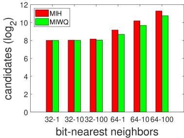
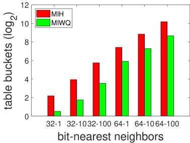
(a) candidates	(b) buckets

Figure 2: Comparison between MIWQ and MIH on SIFT1B.

PQTable

Recently, PQTable (?) is proposed to perform an efficient search for Product Quantization (PQ) (?) which is another encoding method. With some modifications, PQTable can be used for querying from the weighted binary codes. The binary codes are split into disjoint parts each of which consists of continuous 8-bit binary codes. Then, each part can be regarded as a codebook, and PQTable is applied.

Since PQTable and our method both can return the nearest weighted binary codes of the query accurately, we compare them with respect to the running time. As PQTable is also based on the multi-index tables, to further explore the difference between our method and PQTable, our table merge algorithm is applied to PQTable and replaces the table merge algorithm of PQTable, which is dubbed as $\rm{PQTable_{max\_heap}}$. Table 8 shows the time comparison between MIWQ, PQTable and $\rm{PQTable_{max\_heap}}$. According to the results, our table merging algorithm is faster than that of PQTable, which shows that our table merging algorithm can terminate the process by determining whether the $K$-NN of the query have been found faster than that of PQTable. Comparing MIWQ with $\rm{PQTable_{max\_heap}}$, with same table merging algorithm, MIWQ is faster than $\rm{PQTable_{max\_heap}}$, especially for the 32-bit case. As MIWQ and $\rm{PQTable_{max\_heap}}$ both perform the exact $K$-NN search, the order of table buckets to be probed is the same. The difference between them is the process to find the next hash table bucket. Since our method exploits the characteristics of the weighted binary codes, the bucket candidate space to traverse from our method is smaller than that of PQTable. Hence, our method can find the next smallest un-probed binary bucket faster than PQTable.

Table 8: Time cost (ms) on SIFT1B.

bit-$K$ NN	MIWQ	PQTable	$\rm{PQTable_{max\_heap}}$
32-1	6.15	51.31	50.44
32-10	6.31	51.22	50.48
32-100	6.53	51.43	50.55
64-1	7.78	57.26	54.53
64-10	12.65	64.55	61.21
64-100	32.17	92.11	85.33

Conclusion

In this paper, a new querying method is proposed to return the nearest weighted binary codes of the query in a non-exhaustive way. The method consists of two algorithms, the table bucket finding algorithm and the table merging algorithm. The former one is designed to consecutively find the un-probed table buckets, and the latter one is developed to merge the candidates from each table. The experiments show that our method can produce the same querying results as linear scan does with a large time speed-up on the large-scale dataset which includes up to 1 billion data points.

Appendix A

$\mathbb{Corollary}$ $\mathbb{1:}$ Every binary code can be generated by above two operations.

$\mathbb{Proof:}$ It can be proved by mathematical induction.

$\bf{Basis:}$ We have the binary code ${\bf{h}}_{0}$ = $\bf{h}$ which have no changed bits initially. Then by definition, ${\bf{\hat{h}}}_{1}$ is generated by changing the first bit of ${\bf{h}}_{0}$ according to the first operation. It is easy to find that every binary code ${\bf{h}}_{1}$ which have 1 changed bit can be generated from ${\bf{\hat{h}}}_{1}$ according to the second operation.

$\bf{Inductive}$ $\mathbb{step:}$ Assume every binary code ${\bf{h}}_{z}$ which has $z$ changed bits can be generated. For every binary code ${\bf{h}}_{z+1}=[h_{1}\ldots\bar{h}_{i}\ldots\bar{h}_{j}\ldots h_{b}]$ which has $z+1$ changed bits, where the $i^{th}$ bit and the $j^{th}$ bit are the $z^{th}$ and $(z+1)^{th}$ changed bit, respectively. It can be generated by the second operation from another binary code ${\bf{\hat{h}}}_{z+1}=[h_{1}\ldots\bar{h}_{i}\bar{h}_{i+1}\ldots h_{b}]$, where the changed status of the $j^{th}$ bit is moved to the $(i+1)^{th}$ bit. Then ${\bf{\hat{h}}}_{z+1}$ can be generated by the first operation from the binary code ${\bf{\tilde{h}}}_{z}=[h_{1}\ldots\bar{h}_{i}h_{i+1}\ldots h_{j}\ldots h_{b}]$, where the $(i+1)^{th}$ bit is changed back to the previous status and ${\bf{\tilde{h}}}_{z}$ has $z$ changed bits. Thereby, every binary code ${\bf{h}}_{z+1}$ which has $z+1$ changed bits can be generated by two operations from $\mathbb{h}_{z}$.

Appendix B

$\mathbb{Theorem}$ $\mathbb{1:}$ The binary code that has the smallest sum of weights among the un-probed binary codes is always in the priority queue.

$\mathbb{Proof:}$ It can be proved by mathematical induction.

$\bf{Basis:}$ By definition, we have the binary code $\bf{h}$ which have no changed bits initially. It is the smallest among all the binary codes and is pushed into the priority queue.

$\bf{Inductive}$ $\mathbb{step:}$ Assume the top item ${\bf{h}}_{a}$ of the priority queue is the smallest among the current un-probed binary codes. When it is taken out, two new binary codes are constructed and pushed into the queue. Assume there is another binary code ${\bf{h}}_{b}$ which is not in the queue and is smallest among the current un-probed binary codes after ${\bf{h}}_{a}$ is taken out. According to $\mathbb{Corollary}$ $\mathbb{1}$, ${\bf{h}}_{b}$ can be directly generated from ${\bf{h}}_{c}$ by the above two operations. ${\bf{h}}_{c}$ is smaller than ${\bf{h}}_{b}$. Since ${\bf{h}}_{b}$ is smallest among the current un-probed binary codes, ${\bf{h}}_{c}$ should have been probed. If ${\bf{h}}_{c}$ is probed and ${\bf{h}}_{b}$ is generated from ${\bf{h}}_{c}$, ${\bf{h}}_{b}$ should have been pushed into the queue. Obviously, the assumption is invalid. So the binary code which has smallest sum of weights among the un-probed binary codes is always in the priority queue.

Appendix C

$\mathbb{Theorem}$ $\mathbb{2:}$ The binary codes that are found and stored in the max-heap have the smallest sum of weights among all binary codes.

$\mathbb{Proof:}$ This can be proved by contradiction. Assume there exists an identifier that is not found yet and its corresponding binary code is $\mathbb{\tilde{r}}$. Its sum of weights $g(\mathbb{\tilde{r}})$ (the definition of the function $g()$ is in Eqn.(7) in the manuscript) is smaller than that of the root node $\mathbb{r}$ in the max-heap ($i.e.$ $g(\mathbb{\tilde{r}})<g(\mathbb{r})$). Since $g({\bf{r}})\leq S$ (the definition of $S$ is provided in Eqn.(8) in the manuscript) and $g({\bf{\tilde{r}}})<g({\bf{r}}),$ $g({\bf{\tilde{r}}})<S$. Then, at least one of the disjoint substrings of $\mathbb{\tilde{r}}$ is smaller than the top substring of the corresponding queue. This substring should have been taken out from the queue. Since the substring is taken out as a bucket to be probed, $\mathbb{\tilde{r}}$ should have been inserted into the max-heap. Obviously the assumption is invalid. Therefore, the binary codes that are found and stored in the max-heap have the smallest sum of weights among all binary codes.

Appendix D

To evaluate the efficiency and the accuracy of the querying methods on different weighted binary codes, the classical data-independent hashing algorithm Locality-Sensitive Hashing (LSH) (?) and the classical data-dependent hashing algorithm Iterative Quantization (ITQ) (?) are used to map high-dimensional vectors into binary codes, and two weighted hashing method, Asymmetric Distance (Asym) (?) and Weighted Hamming distance (Wh) (?), are adopted to generate the weights for each bit of binary codes.

The average time for the query with different binary codes and different weights are shown from Table 9 to Table 12. From the results, we can see that MIH and MIWQ are both faster than Linear Scan in all the cases. MIWQ is comparable or a litter inferior to MIH in the average time.

Table 9: The average time for the query on Places205 with Asym.

	bit	method	speed-up factors for $K$-NN
			1-NN		10-NN		100-NN
			time(ms)	speed-up factor	time(ms)	speed-up factor	time(ms)	speed-up factor
LSH	32	Linear Scan	23.06	1.0	23.06	1.0	23.06	1.0
		MIH	0.11	209.6	0.21	109.8	0.52	44.3
		$\bf{MIWQ}$	$\bf{0.11}$	$\bf{209.6}$	$\bf{0.21}$	$\bf{109.8}$	$\bf{0.55}$	$\bf{41.9}$
	64	Linear Scan	33.83	1.0	33.83	1.0	33.83	1.0
		MIH	0.51	66.3	1.03	32.84	2.4	14.0
		$\bf{MIWQ}$	$\bf{0.63}$	$\bf{53.6}$	$\bf{1.42}$	$\bf{23.82}$	$\bf{3.65}$	$\bf{9.2}$
ITQ	32	Linear Scan	18.81	1.0	18.81	1.0	18.81	1.0
		MIH	0.08	235.1	0.11	171.0	0.23	81.7
		$\bf{MIWQ}$	$\bf{0.08}$	$\bf{235.1}$	$\bf{0.12}$	$\bf{156.7}$	$\bf{0.28}$	$\bf{67.1}$
	64	Linear Scan	29.9	1.0	29.9	1.0	29.9	1.0
		MIH	0.28	106.7	0.52	57.5	1.1	27.1
		$\bf{MIWQ}$	$\bf{0.39}$	$\bf{76.6}$	$\bf{0.8}$	$\bf{37.3}$	$\bf{1.91}$	$\bf{15.6}$

Table 10: The average time for the query on Places205 with Wh.

	bit	method	speed-up factors for $K$-NN
			1-NN		10-NN		100-NN
			time(ms)	speed-up factor	time(ms)	speed-up factor	time(ms)	speed-up factor
LSH	32	Linear Scan	24.43	1.0	24.43	1.0	24.43	1.0
		MIH	0.11	222.0	0.21	116.3	0.52	46.9
		$\bf{MIWQ}$	$\bf{0.11}$	$\bf{222.0}$	$\bf{0.21}$	$\bf{116.3}$	$\bf{0.54}$	$\bf{45.2}$
	64	Linear Scan	46.23	1.0	46.23	1.0	46.23	1.0
		MIH	0.51	90.6	1.03	44.8	2.4	19.2
		$\bf{MIWQ}$	$\bf{0.62}$	$\bf{74.5}$	$\bf{1.39}$	$\bf{33.2}$	$\bf{3.58}$	$\bf{12.9}$
ITQ	32	Linear Scan	24.71	1.0	24.71	1.0	24.71	1.0
		MIH	0.08	308.8	0.11	224.6	0.23	107.4
		$\bf{MIWQ}$	$\bf{0.08}$	$\bf{308.8}$	$\bf{0.12}$	$\bf{205.9}$	$\bf{0.3}$	$\bf{82.3}$
	64	Linear Scan	46.21	1.0	46.21	1.0	46.21	1.0
		MIH	0.28	165.0	0.52	88.8	1.1	42.0
		$\bf{MIWQ}$	$\bf{0.41}$	$\bf{112.7}$	$\bf{0.86}$	$\bf{53.7}$	$\bf{2.05}$	$\bf{22.5}$

Table 11: The average time for the query on GIST1M with Asym.

	bit	method	speed-up factors for $K$-NN
			1-NN		10-NN		100-NN
			time(ms)	speed-up factor	time(ms)	speed-up factor	time(ms)	speed-up factor
LSH	32	Linear Scan	22.17	1.0	22.17	1.0	22.17	1.0
		MIH	0.1	221.7	0.16	138.5	0.37	59.9
		$\bf{MIWQ}$	$\bf{0.12}$	$\bf{184.7}$	$\bf{0.25}$	$\bf{88.6}$	$\bf{0.77}$	$\bf{28.7}$
	64	Linear Scan	39.36	1.0	39.36	1.0	39.36	1.0
		MIH	0.87	45.2	1.65	23.8	3.15	12.4
		$\bf{MIWQ}$	$\bf{1.84}$	$\bf{21.3}$	$\bf{3.9}$	$\bf{10.0}$	$\bf{8.17}$	$\bf{4.8}$
ITQ	32	Linear Scan	22.09	1.0	22.09	1.0	22.09	1.0
		MIH	0.16	138.0	0.3	73.6	0.69	32.0
		$\bf{MIWQ}$	$\bf{0.17}$	$\bf{129.9}$	$\bf{0.33}$	$\bf{66.9}$	$\bf{0.84}$	$\bf{26.2}$
	64	Linear Scan	38.71	1.0	38.71	1.0	38.71	1.0
		MIH	1.35	28.6	2.6	14.8	5.04	7.6
		$\bf{MIWQ}$	$\bf{2.14}$	$\bf{18.0}$	$\bf{4.55}$	$\bf{8.5}$	$\bf{9.66}$	$\bf{4.0}$

Table 12: The average time for the query on GIST1M with Wh.

	bit	method	speed-up factors for $K$-NN
			1-NN		10-NN		100-NN
			time(ms)	speed-up factor	time(ms)	speed-up factor	time(ms)	speed-up factor
LSH	32	Linear Scan	23.93	1.0	23.93	1.0	23.93	1.0
		MIH	0.1	239.3	0.16	149.5	0.37	64.6
		$\bf{MIWQ}$	$\bf{0.12}$	$\bf{199.4}$	$\bf{0.26}$	$\bf{92.0}$	$\bf{0.78}$	$\bf{30.6}$
	64	Linear Scan	38.52	1.0	38.52	1.0	38.52	1.0
		MIH	0.87	44.2	1.65	23.3	3.15	12.2
		$\bf{MIWQ}$	$\bf{1.92}$	$\bf{20.0}$	$\bf{4.06}$	$\bf{9.4}$	$\bf{8.52}$	$\bf{4.5}$
ITQ	32	Linear Scan	22.62	1.0	22.62	1.0	22.62	1.0
		MIH	0.16	141.3	0.3	75.4	0.69	32.7
		$\bf{MIWQ}$	$\bf{0.18}$	$\bf{125.6}$	$\bf{0.31}$	$\bf{72.9}$	$\bf{0.89}$	$\bf{25.4}$
	64	Linear Scan	43.72	1.0	43.72	1.0	43.72	1.0
		MIH	1.35	32.3	2.6	16.8	5.04	8.6
		$\bf{MIWQ}$	$\bf{2.17}$	$\bf{20.1}$	$\bf{4.82}$	$\bf{9.0}$	$\bf{9.91}$	$\bf{4.4}$

The precision results of the querying methods with different binary codes and different weights are shown from Table 13 to Table 16. According to the results, MIH can achieve higher search accuracy than Baseline, but is inferior to MIWQ. As MIH cannot return the $K$ nearest weighted binary codes accurately, MIH is inferior to MIWQ. Since MIWQ achieves the same search accuracy as Linear Scan, it shows that MIWQ can return the $K$ nearest weighted binary codes of the query accurately.

Table 13: The precision results on Places205 with binary codes generated by LSH.

bit	method	precision ($\%$)
		Asym			Wh
		1-NN	10-NN	100-NN	1-NN	10-NN	100-NN
32	Baseline	21.56	22.23	19.83	21.56	22.23	19.83
	MIH	22.81	23.20	20.86	22.70	23.22	20.90
	Linear Scan	25.29	24.97	22.64	25.58	24.98	22.71
	$\mathbb{MIWQ}$	$\bf{25.29}$	$\bf{24.97}$	$\bf{22.64}$	$\bf{25.58}$	$\bf{24.98}$	$\bf{22.71}$
64	Baseline	31.17	29.71	26.67	31.17	29.71	26.67
	MIH	31.41	30.27	27.46	31.31	30.31	27.49
	Linear Scan	34.46	31.96	28.72	34.34	31.87	28.88
	$\mathbb{MIWQ}$	$\bf{34.46}$	$\bf{31.96}$	$\bf{28.72}$	$\bf{34.34}$	$\bf{31.87}$	$\bf{28.88}$

Table 14: The precision results on Places205 with binary codes generated by ITQ.

bit	method	precision ($\%$)
		Asym			Wh
		1-NN	10-NN	100-NN	1-NN	10-NN	100-NN
32	Baseline	22.52	23.85	22.40	22.52	23.85	22.40
	MIH	23.32	24.86	23.12	23.41	24.89	23.12
	Linear Scan	24.96	26.19	24.42	24.90	26.22	24.41
	$\mathbb{MIWQ}$	$\bf{24.96}$	$\bf{26.19}$	$\bf{24.42}$	$\bf{24.90}$	$\bf{26.22}$	$\bf{24.41}$
64	Baseline	32.76	31.53	28.91	32.76	31.53	28.91
	MIH	33.34	32.14	29.53	36.68	35.63	32.66
	Linear Scan	35.02	33.50	30.69	38.81	36.81	33.55
	$\mathbb{MIWQ}$	$\bf{35.02}$	$\bf{33.50}$	$\bf{30.69}$	$\bf{38.81}$	$\bf{36.81}$	$\bf{33.55}$

Table 15: The precision results on GIST1M with binary codes generated by LSH.

bit	method	precision ($\%$)
		Asym			Wh
		1-NN	10-NN	100-NN	1-NN	10-NN	100-NN
32	Baseline	11.90	7.57	5.11	11.90	7.57	5.11
	MIH	12.10	8.46	5.92	11.80	8.12	5.74
	Linear Scan	13.20	9.94	7.31	13.50	9.75	7.04
	$\mathbb{MIWQ}$	$\bf{13.20}$	$\bf{9.94}$	$\bf{7.31}$	$\bf{13.50}$	$\bf{9.75}$	$\bf{7.04}$
64	Baseline	21.10	14.47	10.16	21.10	14.47	10.16
	MIH	21.50	16.11	11.55	21.70	15.63	11.26
	Linear Scan	24.90	19.14	13.65	23.90	18.30	13.36
	$\mathbb{MIWQ}$	$\bf{24.90}$	$\bf{19.14}$	$\bf{13.65}$	$\bf{23.90}$	$\bf{18.30}$	$\bf{13.36}$

Table 16: The precision results on GIST1M with binary codes generated by ITQ.

bit	method	precision ($\%$)
		Asym			Wh
		1-NN	10-NN	100-NN	1-NN	10-NN	100-NN
32	Baseline	30.80	21.58	14.68	30.80	21.58	14.68
	MIH	29.50	23.29	16.76	30.50	22.58	16.35
	Linear Scan	33.80	26.69	19.70	34.2	26.01	19.06
	$\mathbb{MIWQ}$	$\bf{33.80}$	$\bf{26.69}$	$\bf{19.70}$	$\bf{34.2}$	$\bf{26.01}$	$\bf{19.06}$
64	Baseline	39.60	30.15	20.71	39.60	30.15	20.71
	MIH	40.40	33.69	24.02	39.80	32.13	22.92
	Linear Scan	47.00	38.40	27.41	45.50	36.29	26.43
	$\mathbb{MIWQ}$	$\bf{47.00}$	$\bf{38.40}$	$\bf{27.41}$	$\bf{45.50}$	$\bf{36.29}$	$\bf{26.43}$

References

- [Andoni and Indyk 2006] Andoni, A., and Indyk, P. 2006. Near-optimal hashing algorithms for approximate nearest neighbor in high dimensions. In 47th Annual IEEE Symposium on Foundations of Computer Science, 459–468.
- [Babenko and Lempitsky 2015] Babenko, A., and Lempitsky, V. 2015. The inverted multi-index. IEEE TPAMI 37(6):1247–1260.
- [Balntas, Tang, and Mikolajczyk 2018] Balntas, V.; Tang, L.; and Mikolajczyk, K. 2018. Binary online learned descriptors. IEEE TPAMI 40(3):555–567.
- [Cakir et al. 2017] Cakir, F.; He, K.; Bargal, S. A.; and Sclaroff, S. 2017. Mihash: Online hashing with mutual information. In ICCV, 437–445.
- [Duan et al. 2015] Duan, L. Y.; Lin, J.; Wang, Z.; Huang, T.; and Gao, W. 2015. Weighted component hashing of binary aggregated descriptors for fast visual search. IEEE TMM 17(6):828–842.
- [Fan et al. 2013] Fan, B.; Kong, Q.; Yuan, X.; Wang, Z.; and Pan, C. 2013. Learning weighted hamming distance for binary descriptors. In ICASSP, 2395–2399.
- [Gong et al. 2013] Gong, Y.; Lazebnik, S.; Gordo, A.; and Perronnin, F. 2013. Iterative quantization: A procrustean approach to learning binary codes for large-scale image retrieval. IEEE TPAMI 35(12):2916–2929.
- [Gordo et al. 2014] Gordo, A.; Perronnin, F.; Gong, Y.; and Lazebnik, S. 2014. Asymmetric distances for binary embeddings. IEEE TPAMI 36(1):33–47.
- [Huang, Wei, and Zhang 2017] Huang, Z.; Wei, Z.; and Zhang, G. 2017. Rwbd: Learning robust weighted binary descriptor for image matching. IEEE TCSVT PP(99):1–1.
- [Jegou, Douze, and Schmid 2011] Jegou, H.; Douze, M.; and Schmid, C. 2011. Product quantization for nearest neighbor search. IEEE TPAMI 33(1):117–128.
- [Krizhevsky, Sutskever, and Hinton 2012] Krizhevsky, A.; Sutskever, I.; and Hinton, G. E. 2012. Imagenet classification with deep convolutional neural networks. In NeurIPS, 1097–1105.
- [Leutenegger, Chli, and Siegwart 2011] Leutenegger, S.; Chli, M.; and Siegwart, R. Y. 2011. Brisk: Binary robust invariant scalable keypoints. In ICCV, 2548–2555.
- [Li et al. 2019] Li, C.; Deng, C.; Wang, L.; Xie, D.; and Liu, X. 2019. Coupled cyclegan: Unsupervised hashing network for cross-modal retrieval. In AAAI, 176–183.
- [Lin et al. 2019] Lin, M.; Ji, R.; Liu, H.; Sun, X.; Wu, Y.; and Wu, Y. 2019. Towards optimal discrete online hashing with balanced similarity. In AAAI, 8722–8729.
- [Liu et al. 2014] Liu, W.; Mu, C.; Kumar, S.; and Chang, S.-F. 2014. Discrete graph hashing. In NeurIPS, 3419–3427.
- [Liu et al. 2019] Liu, H.; Ji, R.; Wang, J.; and Shen, C. 2019. Ordinal constraint binary coding for approximate nearest neighbor search. IEEE TPAMI 41(4):941–955.
- [Lowe 2004] Lowe, D. G. 2004. Distinctive image features from scale-invariant keypoints. IJCV 60(2):91–110.
- [Matsui, Yamasaki, and Aizawa 2018] Matsui, Y.; Yamasaki, T.; and Aizawa, K. 2018. Pqtable: Nonexhaustive fast search for product-quantized codes using hash tables. IEEE TMM 20(7):1809–1822.
- [Norouzi, Punjani, and Fleet 2014] Norouzi, M.; Punjani, A.; and Fleet, D. J. 2014. Fast exact search in hamming space with multi-index hashing. IEEE TPAMI 36(6):1107–1119.
- [Oliva and Torralba 2001] Oliva, A., and Torralba, A. 2001. Modeling the shape of the scene: A holistic representation of the spatial envelope. IJCV 42(3):145–175.
- [Rublee et al. 2011] Rublee, E.; Rabaud, V.; Konolige, K.; and Bradski, G. 2011. Orb: An efficient alternative to sift or surf. In ICCV, 2564–2571.
- [Song et al. 2018] Song, J.; He, T.; Gao, L.; Xu, X.; Hanjalic, A.; and Shen, H. T. 2018. Binary generative adversarial networks for image retrieval. In AAAI, 394–401.
- [Torralba, Fergus, and Freeman 2008] Torralba, A.; Fergus, R.; and Freeman, W. T. 2008. 80 million tiny images: A large data set for nonparametric object and scene recognition. IEEE TPAMI 30(11):1958–1970.
- [Wang et al. 2018] Wang, J.; Zhang, T.; Song, J.; Sebe, N.; and Shen, H. T. 2018. A survey on learning to hash. IEEE TPAMI 40(4):769–790.
- [Weng et al. 2016] Weng, Z.; Yao, W.; Sun, Z.; and Zhu, Y. 2016. Asymmetric distance for spherical hashing. In ICIP, 206–210.
- [Zhang et al. 2013] Zhang, L.; Zhang, Y.; Tang, J.; Lu, K.; and Tian, Q. 2013. Binary code ranking with weighted hamming distance. In CVPR, 1586–1593.
- [Zhou et al. 2014] Zhou, B.; Lapedriza, A.; Xiao, J.; Torralba, A.; and Oliva, A. 2014. Learning deep features for scene recognition using places database. In NeurIPS, 487–495.