Dynamics of Laterally Propagating Flames in X-ray Bursts. I. Burning Front Structure

Abstract

We investigate the structure of laterally-propagating flames through the highly-stratified burning layer in an X-ray burst. Two-dimensional hydrodynamics simulations of flame propagation are performed through a rotating plane-parallel atmosphere, exploring the structure of the flame. We discuss the approximations needed to capture the length and time scales at play in an X-ray burst and describe the flame acceleration observed. Our studies complement other multidimensional studies of burning in X-ray bursts.

1 Introduction

X-ray bursts (XRBs) are thermonuclear explosions in an accreted H or He layer on the surface of a neutron star (see Galloway & Keek 2017 for a review). Observations of bursts can assist in constraining the properties of the underlying neutron star, helping to illuminate the nuclear equation of state (Steiner et al., 2010; Özel & Freire, 2016). Extensive observations of brightness oscillations during the rise (the initial phase of the burst where the observed flux rapidly increases) have provided evidence that the burning begins in a localized region and spreads over the surface of the neutron star (Bhattacharyya & Strohmayer, 2006, 2007; Chakraborty & Bhattacharyya, 2014).

One dimensional studies of XRBs have been very successful in predicting the lightcurves and recurrence times (see, e.g., Woosley et al. 2004). These assume spherical symmetry and thus cannot capture the effects of localized burning spreading across the neutron star. These studies have also been used to explore the sensitivity of the burst observables to accretion and reaction rates (Cyburt et al., 2010a; José et al., 2010; Lampe et al., 2016), and to model individual bursts (Johnston et al., 2019).

Multidimensional simulations of burning on a neutron star are more difficult, with both the temporal and spatial scales presenting challenges (see Zingale et al. 2018 for an overview). For the spatial scales, we need to resolve the reaction zone, $\mathcal{O}(10~{}\mbox{cm})$ or smaller, the scale height of the atmosphere, $\mathcal{O}(500~{}\mbox{cm})$, and the Rossby scale where the Coriolis force balances the lateral pressure gradient, $\mathcal{O}(10^{5}~{}\mbox{cm})$ (Spitkovsky et al., 2002). For the temporal scales, capturing the rise, $\mathcal{O}(1~{}\mbox{s})$, and the decay of the burst, $\mathcal{O}(10~{}\mbox{s})$, as well as the accretion period between bursts, $\mathcal{O}(10^{4}~{}\mbox{s})$, is currently beyond the ability of multidimensional hydro codes. Nevertheless, significant progress has been made in understanding the multidimensional nature of XRBs, through various approximations.

Laterally propagating detonations were modeled by Fryxell & Woosley (1982) and Zingale et al. (2001). However, since it is difficult to detonate helium at the densities found in normal XRBs, and even harder to detonate hydrogen because of the waiting times for weak reactions, these would only occur at very high densities. This means that detonations may only really be applicable to superbursts (where carbon is the reactant) (Weinberg et al., 2006; Weinberg & Bildsten, 2007).

Global multidimensional studies were performed by Spitkovsky et al. (2002), where it was demonstrated that the Coriolis force plays an important role in confining the burning as it spreads across the neutron star surface. These calculations used the shallow-water approximation, so the vertical details of the atmosphere’s structure were not captured. Their model showed that the horizontal pressure gradient between the ash and fuel can be important in accelerating the burning front.

Small-domain studies of convective burning in XRBs preceding flame development have been done in two-dimensions (Lin et al., 2006; Malone et al., 2011, 2014) and three-dimensions (Zingale et al., 2015). These calculations used low Mach number methods, which approximate the hydrodynamics equations to filter soundwaves, enabling large timesteps and efficient modeling of subsonic convection. While these calculations could not support the lateral differences needed for flame spreading, they can help understand the role that convection plays in distributing the initial burning products vertically throughout the neutron star atmosphere as well as the nature of any turbulence the burning front might encounter as it propagates through the atmosphere.

The first vertically resolved simulations of lateral deflagrations were obtained by Cavecchi et al. (2013), who showed how the Coriolis force creates a geometrical configuration that increases the flame speed set by conduction by a factor $\sim L_{R}/H$, where $L_{R}$ is the Rossby radius and $H$ is the scale height of the burning layer. The effect of changing Coriolis confinement across the surface on the flame propagation was explored in Cavecchi et al. (2015), while Cavecchi et al. (2016) showed how magnetic field tension, opposing the Coriolis force, can either speed up or slow down the flame by changing the horizontal extent of the flame front. Finally, Cavecchi & Spitkovsky (2019) studied the effects in 3D of the baroclinic instability at the flame front, measuring flames up to 10 times faster than in the 2D case.

For deflagrations, we either need to resolve the structure of the reaction zone or use a flame model. Flame models usually assume that the flame structure is thin compared to the size of the system (see, e.g., Röpke et al. (2007) for applications to Type Ia supernovae). For XRBs however, the flame thickness is comparable to the scale height of the atmosphere, so we cannot use these approximations. Accurate models of flames in XRBs therefore require that we resolve the thermal width, which is $\mathcal{O}(10~{}\mbox{cm})$ for helium flames (Timmes, 2000).

The goal of this study is to understand what numerical and physical approximations are required to perform a full hydrodynamical, multidimensional simulation of flame propagation through the atmosphere of a neutron star. For simplicity in this first set of calculations, we will use a pure helium composition. These studies complement the prior multidimensional studies described above in helping us to build a picture of the dynamics of X-ray bursts.

2 Numerical Approach

All simulations are performed with the Castro hydrodynamics code (Almgren et al. 2010; see also Zingale et al. 2017 for a recent description). We evolve the system of fully compressible Euler equations for reacting flow:

$$\frac{\partial(\rho X_{k})}{\partial t} = -\nabla\cdot(\rho{\bf{U}}X_{k})+\rho\dot{\omega}_{k}$$ (1)

$$\frac{\partial(\rho{\bf{U}})}{\partial t} = -\nabla\cdot(\rho{\bf{U}}{\bf{U}})-\nabla p+\rho{\bf{g}}$$ (2)

$$-2\rho{\bf{\Omega}}\times{\bf{U}}-\rho{\bf{\Omega}}\times({\bf{\Omega}}\times{\bf{r}})$$

$$\frac{\partial(\rho E)}{\partial t} = -\nabla\cdot(\rho{\bf{U}}E+p{\bf{U}})+\nabla\cdot k_{\rm th}\nabla T+\rho\dot{\epsilon}+$$ (3)

$$\rho{\bf{U}}\cdot{\bf{g}}-\rho({\bf{\Omega}}\cdot{\bf{r}})({\bf{\Omega}}\cdot{\bf{U}})+\rho|{\bf{\Omega}}|^{2}({\bf{U}}\cdot{\bf{r}})$$

Here, $\rho$ is the mass density, ${\bf{U}}$ is the velocity, $p$ is the pressure and $E$ is the specific total energy, which is related to the specific internal energy as $e=E-|{\bf{U}}|^{2}/2$. The forcing in the momentum equation includes gravity, described by gravitational acceleration ${\bf{g}}$, and rotational forces, described by angular velocity ${\bf{\Omega}}$, with ${\bf{r}}$ the position vector from the origin. Species are described by mass fractions, $X_{k}$ (such that $\sum_{k}X_{k}=1$), and creation rates, $\dot{\omega}$, and are related to the total specific energy generation rate, $\dot{\epsilon}$. The total mass conservation,

$$\frac{\partial\rho}{\partial t}=-\nabla\cdot(\rho{\bf{U}})$$ (4)

implies $\sum_{k}\dot{\omega}_{k}=0$. An equation of state of the form $p=p(\rho,e,X_{k})$ completes the thermodynamic description of the system. Thermal diffusion is described by a thermal conductivity $k_{\rm th}$ and temperature $T$.

Castro uses an unsplit piecewise parabolic method (PPM) with characteristic tracing for solving the hydrodynamics (Colella & Woodward, 1984; Miller & Colella, 2002), generalized to an arbitrary equation of state (Zingale & Katz, 2015). Reactions are incorporated via Strang splitting (Strang, 1968), giving a method that is overall second-order accurate in space and time. Castro uses the AMReX adaptive mesh refinement library (Zhang et al., 2019) to manage a hierarchy of grids at different resolutions.

Since the neutron star rotates, we work in a corotating frame, taking the angular velocity ${\bf{\Omega}}$ to be constant. Further, for the two-dimensional simulations presented here, we work in axisymmetric coordinates, but we advect a third component of velocity, coming out of the simulation plane, that participates in the Coriolis force (sometimes described as a 2.5D simulation). We will take the Castro $x$-coordinate to be the cylindrical radial coordinate with corresponding velocity $u$, the Castro $y$-coordinate to be the cylindrical vertical coordinate with corresponding velocity $v$, and the Castro $z$-coordinate to be the cylindrical azimuthal coordinate, with corresponding velocity $w$. A righthanded coordinate system has positive $w$ pointing out of the page. We will take ${\bf{\Omega}}=\Omega_{0}\hat{\bf y}$ for the angular rotation rate, and ${\bf{g}}=-g\hat{\bf y}$ for the gravitational acceleration, with $g$ constant. With these choices, the Coriolis force is:

$$-2\rho{\bf{\Omega}}\times{\bf{U}}=-2\rho\left(\Omega_{0}w\hat{x}-\Omega_{0}u\hat{z}\right)$$ (5)

We will neglect the centrifugal force—with our plane-parallel geometry, this will act only in the lateral direction, and is not expected to greatly affect the dynamics. Carrying the Coriolis force allows us to capture the geostrophic balance that sets up via lateral hydrostatic equilibrium (Spitkovsky et al., 2002). In the discussions below, we will use the Castro coordinate names, $(x,y)$ in our notation.

Writing the momentum equation in terms of the $u$, $v$, and $w$ components, and neglecting the centrifugal force, we have:

$$\frac{\partial(\rho u)}{\partial t}+\nabla\cdot(\rho u{\bf{U}})+\frac{\partial p}{\partial x} =-2\rho\Omega_{0}w$$ (6)

$$\frac{\partial(\rho v)}{\partial t}+\nabla\cdot(\rho v{\bf{U}})+\frac{\partial p}{\partial y} =-\rho g$$ (7)

$$\frac{\partial(\rho w)}{\partial t}+\nabla\cdot(\rho w{\bf{U}})+\cancelto{0}{\frac{\partial p}{\partial z}} =2\rho\Omega_{0}u$$ (8)

where we cancel $\partial p/\partial z$ because there are no variations in the azimuthal direction. This allows us to recast the $w$-velocity equation as a simple advection equation:

$$\frac{\partial w}{\partial t}+{\bf{U}}\cdot\nabla w=2\Omega_{0}u$$ (9)

In our geometry, the flame will propagate from left to right, so $u$ will be positive and the Coriolis force results in $w>0$ (out of the simulation plane). The algorithmic implementation of rotation in Castro is described in Katz et al. (2016).

We use a general stellar equation of state with nuclei (treated as an ideal gas), photons, and degenerate/relativistic electrons, as described in Timmes & Swesty (2000). To model reactions, we use a 13-isotope alpha chain network derived from the aprox13 network (Timmes, 2019). For one of our runs, we use the smaller 7-isotope network described in Timmes et al. (2000). We integrate the network using the VODE integration package (Brown et al., 1989), and our implementation is provided in the StarKiller Microphysics source (the StarKiller Microphysics Development Team et al., 2019). We note that we do not explicitly model viscosity. The reactions will provide the smallscale cutoff to the instabilities and turbulence at the flame front. We also do not include species diffusion—astrophysical flames tend to have large Lewis numbers, so this is not expected to be important (Timmes & Woosley, 1992). Finally, we use the thermal conductivities described in Timmes (2000).

All simulations use adaptive mesh refinement to refine on the atmosphere (leaving the space between the top of the atmosphere and upper boundary at low resolution). As seen in Figure 1, we use up to 3 refinement levels in addition to the base grid, the first one a factor of 4 finer than the previous and the remaining each a factor of 2 finer than the previous. Castro subcycles in time, so the finer grids are evolved with a finer timestep than the coarse grids. Occasionally, the timestep chosen at the start of a cycle will violate the CFL condition during the advancement of the finer grids. In this case, we restart the finer grid evolution with a smaller timestep, subcycling within the larger timestep hierarchy. We use a CFL number of 0.8 for our simulations. The base grid for our standard simulations is $768\times 192$ zones, and the equivalent finest grid when 3 refinement levels are added would be $12288\times 3072$ zones. Our standard domain is $1.2288\times 10^{5}~{}\mathrm{cm}\times 3.072\times 10^{4}~{}\mathrm{cm}$, corresponding to $10~{}\mathrm{cm}$ resolution on the finest grid. We only refine the fuel layer in the left half of the domain at the highest resolution (and only down to densities of $2.5\times 10^{4}~{}\mathrm{g~{}cm^{-3}}$), since this is where we expect the flame to propagate. At the start of the simulation, $3.4\%$ of the domain is at the finest resolution. This increases to $7.4\%$ by the end of the simulation, because of the increase in the scale height of the atmosphere behind the flame.

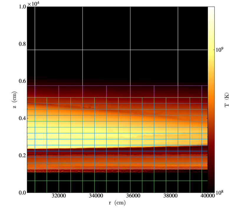
Figure 1: A section of a 2D simulation showing the four-level grid structure. Note that the boxes shown are not the simulation zones, which span $10~{}\mathrm{cm}$ at the finest level, but subdomains containing approximately equal numbers of zones that are distributed across MPI processes. A coarse base grid extending to the upper boundary is drawn in white, with the magenta, green, and blue grids showing the jumps in refinement needed to fully resolve the fuel layer and underlying neutron star.

Thermal diffusion is modeled explicitly, using a predictor-corrector scheme to achieve second-order accuracy. A verification test of the diffusion scheme is shown in Appendix A. The explicit thermal diffusion requires a timestep limiter of the form:

$$\Delta t_{\mathrm{diff}}\leq\frac{1}{2}\frac{\Delta x^{2}}{\mathcal{D}}$$ (10)

where $\mathcal{D}=k_{\rm th}/(\rho c_{v})$ is the thermal diffusivity. The diffusivity increases rapidly at the top of the atmosphere, causing these low density regions to determine the overall timestep for the simulations. Therefore, we disable thermal conduction at low densities where it is not expected to be important.

We use hydrostatic boundary conditions on the lower boundary, using a discretized hydrostatic equilibrium equation of the form:

$$p_{i}=p_{i-1}+\frac{1}{2}\Delta y(\rho_{i}+\rho_{i-1}){\bf{g}}\cdot\hat{\bf y}$$ (11)

and holding the temperature constant in the ghost cells. This is solved together with the equation of state. The velocity is reflected at this boundary. This procedure follows the form described in Zingale et al. (2002). The left boundary is reflecting and the right boundary is a zero-gradient outflow. The top boundary sets the state to simply the conditions in our outer buffer region of the initial model (see below), with the normal velocity set to the larger of zero or the velocity at the top of the domain (this prevents incoming velocities at the top) and the transverse velocities set to zero.

When we begin the simulation, there is a transient phase as the flame gets established. Material that is forced upward will encounter the steep density gradient at the top of the atmosphere and accelerate as it is blown out of the atmosphere. Eventually this material will fall back to the top of the atmosphere. In this paper, we are mostly concerned with the behavior of the flame and not any material that is violently blown out of the top of the atmosphere, so we apply a sponge to this region. This is similar to the method we previously used in Malone et al. (2014), and takes the form of a source term to the momentum and energy equations of the form:

$${\bf S}_{\rho{\bf{U}}} =\rho{\bf{U}}\frac{f}{\Delta t}$$ (12)

$$S_{\rho E} =\rho{\bf{U}}\cdot{\bf S}_{\rho{\bf{U}}}$$ (13)

with the sponge forcing $f$ dependent on the density. We define the sponge shape as:

$$s=\left\{\begin{array}[]{cc}0&\rho>\rho_{\mathrm{upper}}\\ \frac{1}{2}\left[1-\cos\left(\frac{\pi(\rho-\rho_{\mathrm{upper}})}{\Delta\rho}\right)\right]&\rho_{\mathrm{upper}}\geq\rho>\rho_{\mathrm{lower}}\\ 1&\rho<\rho_{\mathrm{lower}}\end{array}\right.$$ (14)

Here $\rho_{\mathrm{upper}}$ and $\rho_{\mathrm{lower}}$ are the densities where the sponge transitions to being fully applied. We take $\rho_{\mathrm{upper}}=10^{2}~{}\mathrm{g~{}cm^{-3}}$ and $\rho_{\mathrm{lower}}=1~{}\mathrm{g~{}cm^{-3}}$, with $\Delta\rho=\rho_{\mathrm{upper}}-\rho_{\mathrm{lower}}$. The sponge update is done implicitly to get the effective forcing, $f$:

$$f=-\left[1-\frac{1}{1+\alpha s}\right]$$ (15)

with $\alpha=\Delta t/\tau_{\mathrm{sponge}}$. Here $\tau_{\mathrm{sponge}}$ is the timescale over which the sponge acts. We take $\tau_{\mathrm{sponge}}=10^{-7}~{}\mathrm{s}$. The sponge drives the velocity of the material in the low density regions at the top of the atmosphere to zero. This sponging helps increase our timestep as well.

3 Flame Properties

The speed and thickness of a laminar helium flame are determined by the energy generation rate and conductivity, and scale roughly as

$$s_{L}\approx\sqrt{k_{\rm th}\dot{\epsilon}}\qquad\lambda_{L}\approx\sqrt{\frac{k_{\rm th}}{\dot{\epsilon}}}$$ (16)

(O’Rourke & Bracco, 1979; Khokhlov, 1993). At the densities we consider in this simulation, the pure He flame speed is quite slow and would require long integration times to see significant evolution of the burning. We therefore consider boosted flames in this first paper, to accelerate the burning and allow us to understand the qualitative effects of laterally propagating flames. To boost the flame while keeping the thickness the same, we can multiply both the burning rate and the conductivity by the same factor. For our standard calculations, we choose 10 for each, to give a 10$\times$ faster flame speed. We call this the “10/10” flame. We will also do a simulation with the reactions and conductivity both boosted by 5, the “5/5” flame.

To understand the time and length scales involved in flame propagation, we do a 1D simulation of a laminar flame using our microphysics. Figure 2 shows the flame thermodynamic profile and properties for the 10/10 flame using our conductivities and the aprox13 reaction network. This flame had a density of $2\times 10^{6}~{}\mathrm{g~{}cm^{-3}}$ and temperature of $5\times 10^{7}$ K. We observe that this flame speed is about $10^{5}~{}\mathrm{cm~{}s^{-1}}$, the flame width is about 40 cm, and it takes about 3 ms to settle into a sustained flame. Note that this speed is quite small compared to the speeds of $\sim 10^{6}~{}\mathrm{cm~{}s^{-1}}$ estimated in Spitkovsky et al. (2002). Table 1 gives the properties of the 10/10 and 5/5 laminar flames. We expect a multidimensional flame to accelerate due to hydrodynamics interactions (wrinkling, turbulence interactions, directed flows feeding fuel into the flame, etc.).

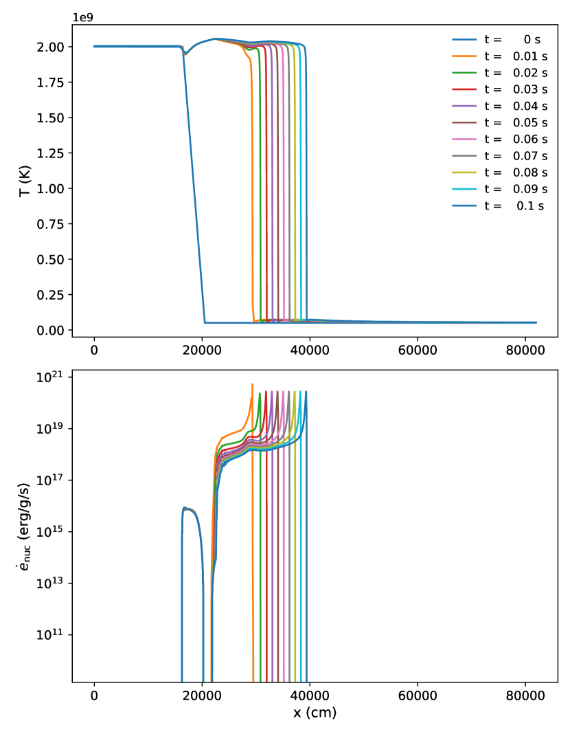
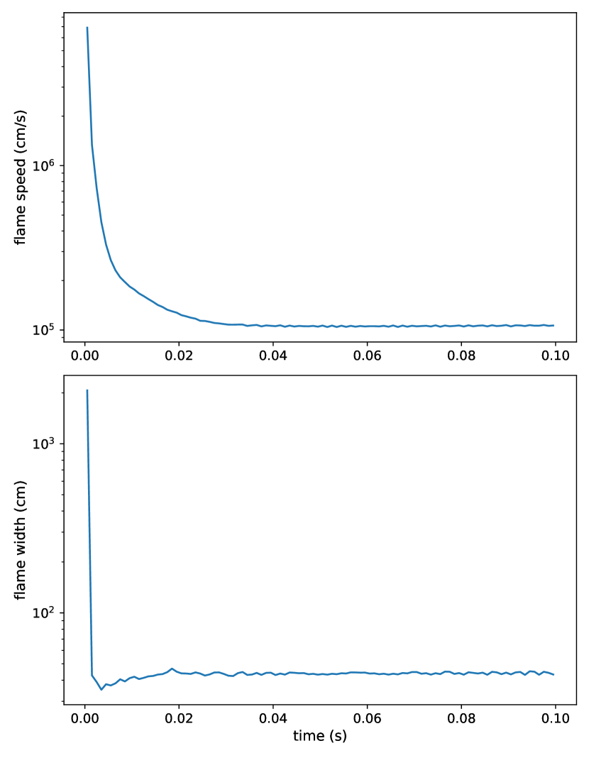
Figure 2: Time-evolution of the 10$\times$ boosted 1D laminar flame. The left plot shows temperature and nuclear energy generation profiles at 11 different times, while the right plot shows flame propagation speed and flame thickness as functions of time.

We measure the laminar flame width as:

$$\lambda_{L}\equiv\frac{\Delta T}{\max\{|\nabla T|\}}$$ (17)

Experience with modeling resolved flames suggests that we need a spatial resolution, $\Delta x$ of $\lambda_{L}/\Delta x\sim 5$ (Bell et al., 2004). These conditions represent the bottom of the He layer. As the density decreases with altitude, the flame thickness increases and the flame speed decreases, so we will easily resolve the flame structure throughout the rest of the atmosphere.

Table 1: Laminar flame speeds.

run	$s_{L}$ (km s-1)
10/10 boost	$1.06\pm 0.01$
5/5 boost	$0.56\pm 0.01$

4 Initial Model

We wish to create an initial atmosphere consisting of a hot “post-flame” region and a cooler atmosphere that the flame will laterally propagate into. We put the hot region at the very left of the domain (the origin of the axisymmetric coordinates). To create these initial conditions, we produce two different hydrostatic models, a “hot” model that will represent the perturbation that drives the flame and a “cool” model that will represent the state ahead of the flame. These will have different scale heights. To create these models, we break the vertical structure of the atmosphere into four layers: (1) the underlying neutron star, (2) a ramp-up to the base of the accreted atmosphere, (3) a fuel layer representing the bulk of the atmosphere where the flame will propagate, and (4) an outer, low density, isothermal buffer above the atmosphere that allows us to capture expansion and explosive dynamics.

The temperature profile in the star and ramp region is given as:

$$T(y)=T_{\star}+\frac{1}{2}(T_{\mathrm{hi}}-T_{\star})\left[1+\tanh\left(\frac{\tilde{y}}{2\delta_{\mathrm{atm}}}\right)\right]$$ (18)

with

$$\tilde{y}=y-H_{\star}-\frac{3}{2}\delta_{\mathrm{atm}}$$ (19)

Here, $\delta_{\mathrm{atm}}$ is a characteristic width of the transition ramp, $T_{\star}$ is the temperature of the neutron star, and $T_{\mathrm{hi}}$ is the highest temperature in the HSE model—it will represent the base of the fuel layer.

The species mass fractions use this same profile, switching from a set describing the underlying star, ${X_{k}}_{\star}$, and the set for the accreted material, ${X_{k}}_{\mathrm{atm}}$, which is used in the isentropic and outer regions. Note, since the profile above is linear in $X$, if the initial mass fractions sum to one, then the blended mass fractions in the ramp region also sum to one.

We specify the density, $\rho_{\mathrm{int}}=\rho(y=H_{\star})$ as the starting point for the integration of hydrostatic equilibrium. This is just below the ramp-up region—this ensures that regardless of what the peak temperature ($T_{\mathrm{hi}}$) is, the state beneath the ramp-up region remains unchanged. Therefore, we will still be in lateral equilibrium in the star region. We will denote the density where $T=T_{\mathrm{hi}}$ as $\rho_{\mathrm{fuel}}$.

Creating the model involves specifying $T_{\star}$, $T_{\mathrm{hi}}$, $T_{\mathrm{lo}}$, $\rho_{\mathrm{int}}$, $H_{\star}$, $\delta_{\mathrm{atm}}$, ${X_{k}}_{\star}$, ${X_{k}}_{\mathrm{atm}}$, and $g$. We then integrate outwards from the base of the ramp region ($y=H_{\star}$), enforcing the discrete form of hydrostatic equilibrium, Eq. 11. Integrating upwards, we find $p_{i}$ and $\rho_{i}$ using a Newton-Raphson solver together with the equation of state, with either the temperature specified, $T_{i}=T(p_{i},\rho_{i},\{X_{k}\}_{i})$ (in the isothermal, ramp, and buffer layers) or constant entropy, $s_{i}=s(p_{i},\rho_{i},\{X_{k}\}_{i})$, in the fuel layer. This follows the procedures described in Zingale et al. (2002). We use a constant temperature for all $y<H_{\star}+3\delta_{\mathrm{atm}}$. Above this, we switch to an isentropic atmosphere until the temperature drops to a floor value, $T_{\mathrm{lo}}$, at which point we again keep the temperature constant. The integration of the atmosphere continues until the density falls to a low density cutoff, $\rho_{\mathrm{cutoff}}$. The material above this height is taken to have constant density and temperature. The choice of factors in front of $\delta_{\mathrm{atm}}$ were designed to make sure the peak $T$ is attained at the desired density of the burning layer. The parameters we use for the model generation are listed in Table 2 and the initial model profiles are showing in Figure 3.

Table 2: Initial model parameters.

parameter	cool	hot
$T_{\star}$	$10^{8}$ K
$T_{\mathrm{hi}}$	$2\times 10^{8}$ K	$1.4\times 10^{9}$ K
$T_{\mathrm{lo}}$	$8\times 10^{6}$ K
$\rho_{\mathrm{int}}$	$3.43\times 10^{6}~{}\mathrm{g~{}cm^{-3}}$
$\rho_{\mathrm{fuel}}$	$2.36\times 10^{6}~{}\mathrm{g~{}cm^{-3}}$	$1.20\times 10^{6}~{}\mathrm{g~{}cm^{-3}}$
$\rho_{\mathrm{cutoff}}$	$10^{-4}~{}\mathrm{g~{}cm^{-3}}$
$H_{\star}$	2000 cm
$\delta_{\mathrm{atm}}$	50 cm
$X_{\star}({}^{56}\mathrm{Ni})\tablenotemark{b}$	1.0
$X_{\mathrm{atm}}({}^{4}\mathrm{He})\tablenotemark{b}$	1.0
${\bf{g}}$	$-1.5\times 10^{14}~{}\mathrm{cm~{}s^{-2}}\hat{\bf y}$

We blend the hot and cold models laterally to produce the perturbation needed to initiate a localized flame, with the hot model at the origin of the axisymmetric geometry. The blending is done as:

$$p(x,y) =f(x)p_{\mathrm{hot}}(y)+[1-f(x)]p_{\mathrm{cool}}(y)$$ (20)

$$\rho(x,y) =f(x)\rho_{\mathrm{hot}}(y)+[1-f(x)]\rho_{\mathrm{cool}}(y)$$ (21)

$$X_{k}(x,y) =f(x){X_{k}}_{\mathrm{hot}}(y)+[1-f(x)]{X_{k}}_{\mathrm{cool}}(y)$$ (22)

with

$$f(x)=\begin{cases}1&x<x_{\mathrm{pert}}\\ 1-\frac{x-x_{\mathrm{pert}}}{\delta_{\mathrm{blend}}}&x_{\mathrm{pert}}\leq x\leq x_{\mathrm{pert}}+\delta_{\mathrm{blend}}\\ 0&x>x_{\mathrm{pert}}+\delta_{\mathrm{blend}}\end{cases}$$ (23)

Since the equation of hydrostatic equilibrium is linear and our blending is a linear combination of two models in hydrostatic equilibrum, the blended model is also in vertical equilibrium initially. We choose $x_{\mathrm{pert}}=1.024\times 10^{4}$ cm and $\delta_{\mathrm{blend}}=2048$ cm. Once the blended model is constructed, we compute $T(x,y)$ and $(\rho e)(x,y)$ from the equation of state,

$$T(x,y) =T(\rho(x,y),p(x,y),X_{k}(x,y))$$ (24)

$$(\rho e)(x,y) =\rho(x,y)\cdot e(\rho(x,y),p(x,y),X_{k}(x,y))$$ (25)

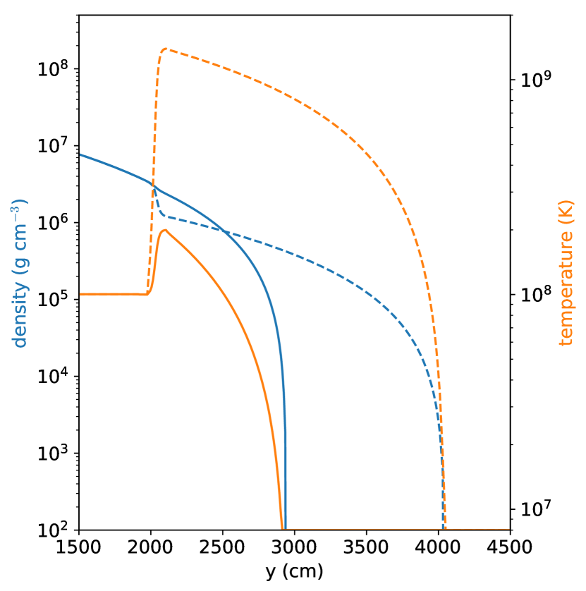
Figure 3: Our “cool” (solid) and “hot” (dashed) initial models, showing both the density and temperature.

The initial model is created on a uniform grid at the resolution corresponding to the finest level of refinement. At regions of the atmosphere that are not refined to the finest level, we interpolate density, pressure, and composition on the grid and then obtain the temperature from the EOS.

5 Simulations and Results

To assess the sensitivity of the flame propagation to the various approximations we made, we ran a suite of simulations. Table 3 summarizes these simulations. The majority of them used a reaction rate boosting of $10$ and a conductivity boosting of $10$, which should increase the flame speed by a factor of $10$. Most simulations used a resolution of $10~{}\mbox{cm}$ and a domain width of a little more than one kilometer. We use an artifically high rotation rate of $2000~{}\mbox{Hz}$, which gives a Rossby length of

$$L_{R}=\frac{\sqrt{gH_{0}}}{\Omega}\sim 3\times 10^{4}~{}\mathrm{cm}$$ (26)

using a scale height $H_{0}=10^{3}~{}\mathrm{cm}$. This is about one quarter of the domain width. The run at $20~{}\mbox{cm}$ resolution used one fewer level of refinement. The slower rotating case (1000 Hz) uses a slightly wider domain to accommodate the expected larger Rossby length. We note that the entire simulation framework for these calculations is freely available in the Castro github repository. In the discussions below, we’ll use the simulation names defined in the table to refer to specific runs and we’ll use the 10/10 run as the reference calculation.

Table 3: Simulation parameters.

name	reaction	conductivity	fine grid	rotation	domain size	network
	boost	boost	resolution	rate
10/10	10	10	10 cm	2000 Hz	$1.2288\times 10^{5}~{}\mbox{cm}\times 3.072\times 10^{4}~{}\mbox{cm}$	aprox13
5/5	5	5	10 cm	2000 Hz	$1.2288\times 10^{5}~{}\mbox{cm}\times 3.072\times 10^{4}~{}\mbox{cm}$	aprox13
10/10-iso7	10	10	10 cm	2000 Hz	$1.2288\times 10^{5}~{}\mbox{cm}\times 3.072\times 10^{4}~{}\mbox{cm}$	iso7
10/10-lowres	10	10	20 cm	2000 Hz	$1.2288\times 10^{5}~{}\mbox{cm}\times 3.072\times 10^{4}~{}\mbox{cm}$	aprox13
10/10-1000 Hz	10	10	10 cm	1000 Hz	$1.8432\times 10^{5}~{}\mbox{cm}\times 3.072\times 10^{4}~{}\mbox{cm}$	aprox13

5.1 General Features

Figure 4 shows the time evolution of the 10/10 simulation, focusing on the mean molecular weight,

$$\bar{A}=\left(\sum_{k}\frac{X_{k}}{A_{k}}\right)^{-1}.$$ (27)

In each frame the buffer of ${}^{56}\mathrm{Ni}$ that serves as the underlying neutron star is seen spanning the bottom of the domain. Above that, the composition begins as pure ${}^{4}\mathrm{He}$, but as the simulation progresses, the flame processes this to heavier nuclei, increasing $\bar{A}$. By about $10~{}\mbox{ms}$, we see the flame front is reasonably well-defined. We see that the bottom of the burning front is lifted off of the base of the atmosphere, greatly increasing the surface area of the burning compared with a perfectly vertical flame front. By $20~{}\mbox{ms}$ the flame has moved out substantially and we are beginning to see a gradient in the composition of the ash, with the heavier nuclei furthest behind the flame. The boosting of the burning likely artificially increases this effect, as we’ll see in the 5/5 case below.

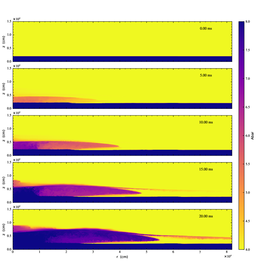
Figure 4: Time series of the mean molecular weight of the flame for our standard 10/10 simulation.

Figure 5 shows the temperature, energy generation rate, and $w$ component of the velocity (the out-of-plane velocity induced by the Coriolis force). This latter field illustrates the hurricane effect set up by the laterally spreading burning front. In the energy generation rate plot, we see that the burning is mostly concentrated toward the bottom of the layer, as expected since the density is greatest there. We see that the peak of the burning has moved off of the symmetry axis, demonstrating that the burning front is propagating to the right. In the temperature plot, we see the effect of our refinement criteria focusing only on the part of the atmosphere where we are most dense, with an artificial change in the temperature at the refinement boundary due in part to the construction of the initial model using the fine grid resolution for HSE. As we will see in the lower resolution case, this does not affect the results.

A final feature worth noting is the ash that seems to move along the surface at a higher velocity than the flame, via surface gravity waves. The sponging that we perform is likely damping this to some extent, and the method by which we initialize the flame may induce a larger transient than in nature. Nevertheless, this surface ash is intriguing because it affects the composition of the photosphere ahead of the burning front, potentially changing our interpretation of observations. This is something that will be explored more fully in the future.

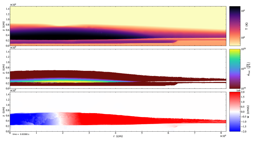
Figure 5: Temperature, energy generation rate, and out-of-plane velocity for the 10/10 simulation at 20 ms.

Our default resolution puts $\sim 80$ zones vertically in the “cool” model atmosphere height. To understand the effects of resolution, we also performed a run with one fewer refinement level, giving a $20~{}\mbox{cm}$ resolution overall (this is our 10/10-lowres run). Figure 6 shows the fields for this run at 20 ms. The structure is largely the same as the 10/10 run, with largely the same flame shape and position, and the same structure in the energy generation rate. Since we do not have a jump in refinement right below the atmosphere, we don’t see the temperature feature from the initial model mapping there, but we do see some cooling in the ${}^{56}\mathrm{Ni}$ region. This is likely a resolution effect, again due to the strong gradient in temperature at the base of the atmosphere. The strong agreement in the low resolution run to the 10/10 run gives us confidence that we are capturing the flame physics properly.

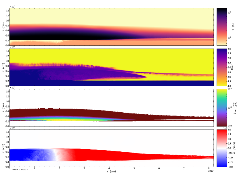
Figure 6: Temperature, mean molecular weight, energy generation rate, and out-of-plane velocity for the 10/10 low resolution simulation at 20 ms.

5.2 Effects of our Approximations

The results above all used a boosting of 10/10. To see how the results are sensitive to this boosting, we ran a simulation with a reduced boosting of 5/5. This is shown in Figure 7. The results look qualitatively the same—a laterally propagating flame develops that is lifted off of the bottom of the fuel layer. The flame has not moved out as far as in the 10/10 simulation, simply because there is less energy release, but we expect that if we were to run this out twice as long, the flame would have advanced to the position seen in our 10/10 runs. The ash is also not as evolved to as high of an $\bar{A}$. The good agreement in the structure of the flame seen with the lower boosting gives us confidence that the overall aspects of the flame structure and acceleration we are seeing are robust to the approximations we make.

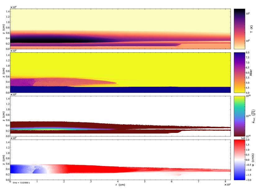
Figure 7: Temperature, mean molecular weight, energy generation rate, and out-of-plane velocity for the 5/5 simulation at 20 ms.

We also considered the effect of the network size. Figure 8 shows a comparison of the 10/10 boosting run with the standard 13-isotope aprox13 network and the reduced 7-isotope iso7 network. We see that the flame in the aprox13 case is slightly more advanced and has a higher $\bar{A}$ than the iso7 case. We see in the next section that these two networks give largely the same flame speed. The reduced network size saves a lot of memory, which will be useful when we transition to 3D simulations.

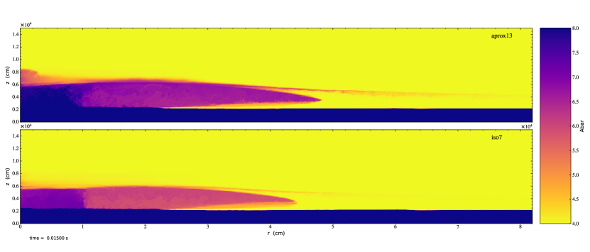
Figure 8: Mean molecular weight at 15 ms comparing a run with aprox13 to a run with the iso7 network.

The final approximation to explore is our choice of rotation rate. We ran the 10/10-1000 Hz simulation for 12.6 ms (shorter than the 20 ms we used for the other runs). We also used a larger domain, $1.8432\times 10^{5}~{}\mathrm{cm}\times 3.072\times 10^{4}~{}\mathrm{cm}$ to account for the larger Rossby radius. Figure 9 shows the flame structure. Overall it looks much like the faster rotator. In the next section, we explore the effect of rotation on the flame acceleration.

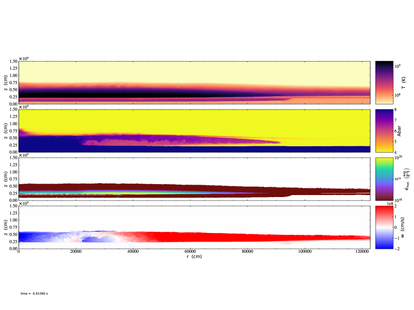
Figure 9: Temperature, mean molecular weight, energy generation rate, and out-of-plane velocity for the 10/10-1000 Hz simulation at 12.6 ms.

5.3 Flame Propagation

To measure the propagation rate of the burning front, we first collapse our nuclear energy generation rate ($\dot{e}_{\mathrm{nuc}}$) data at each time into a 1D radial profile by averaging over the vertical coordinate. We then take the peak $\dot{e}_{\mathrm{nuc}}$ value across all profiles to provide a fixed reference point. We define the position of the flame front to be the location ahead of hottest part of the flame where $\dot{e}_{\mathrm{nuc}}$ first drops to $<0.1\%$ of the global maximum. This corresponds roughly to the leading edge of the burning region. Averaging over the vertical coordinate helps to reduce sensitivity to localized fluid motions, as does tracking the $0.1\%$ contour rather than a local maximum. As we see in Figure 10, the flame settles into a state of steady propagation after an initial transient period spanning $\sim 3$ ms. The position data here are well fitted by a linear function of time, and the resulting slope gives the velocity of the flame front.

Table 4: Flame speeds measured in 2D calculations.

run	$s_{\mathrm{front}}$ (km s-1)
10/10	$9.18\pm 0.03$
5/5	$4.00\pm 0.01$
10/10-iso7	$7.56\pm 0.02$
10/10-lowres	$9.33\pm 0.04$
10/10-1000 Hz	$18.6\pm 0.16$

Table 4 gives the flame speed measured in each multidimensional simulation. The 2D flames propagate at speeds about an order of magnitude faster than their 1D counterparts (Table 1). The increase in flame speed is likely a product of the larger flame surface area and hydrodynamical effects such as turbulence, wrinkling, and convective cycles, which bring cooler fuel from ahead of the front into the hottest part of the burning region.

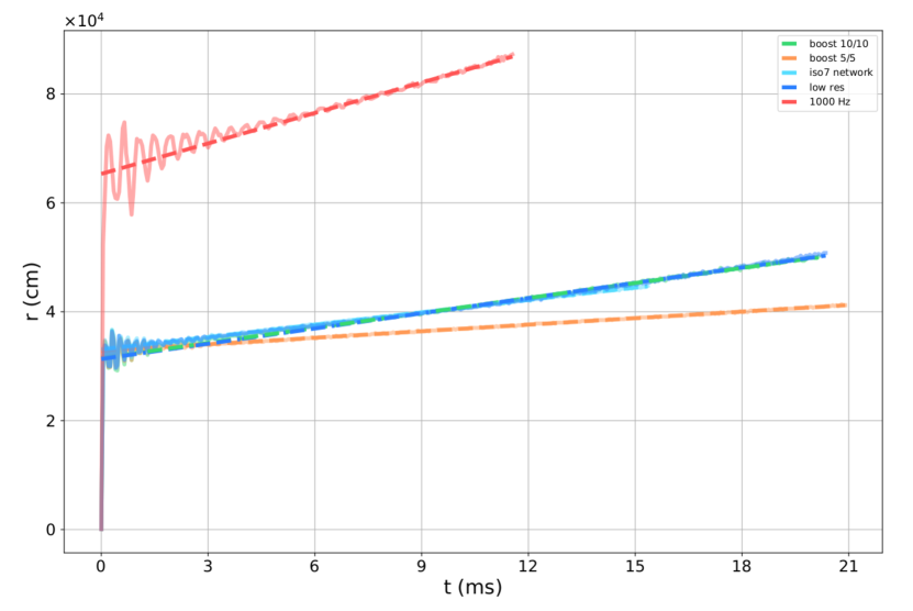
Figure 10: The position of the burning front for each simulation run as a function of time. The dashed lines show linear least squares fits for $t\gtrsim 6$ ms.

All of the various approximations have the expected effects. The flame in the 5/5 boost run propagates at about half the speed of the 10/10 flame. This is consistent with the 1D laminar flames, and is the behavior predicted by Eq. 16. The 1000 Hz run goes 2 times faster than the 10/10 2000 Hz run, as expected from the inverse relation between rotation rate and the ratio of burning front area to scale height (Cavecchi et al., 2013). This confirms that the role of the Coriolis force is to limit the rate of flame spreading by the anticipated geometrical/hydrodynamical effect ($s_{\mathrm{front}}=s_{L}*L_{R}/H$). Reducing the resolution had minimal impact on the flame speed – the low resolution line is right on top of the fit for the standard run in Figure 10, with their slopes differing by only a few percent. Using a smaller network also produces similar behavior to the standard run, although there is a small reduction in speed owing to less energetic burning.

5.4 Entrainment, Flow Features

We explore the baroclinic instability by looking at the magnitude of the baroclinicity, calculated as

$$\boldsymbol{\psi}=\frac{1}{\rho^{2}}\mathbf{\nabla}p\times\mathbf{\nabla}\rho,$$ (28)

and shows the misalignment of the local density and pressure gradients (we also explored this in (Malone et al., 2014)). As we are considering a 2D system, the component of the baroclinicity we consider here (out of the plane) reflects the misalignment of the fields in the plane of the simulation. Figure 11 shows that the baroclinicity peaks along the flame front. This baroclinicity generates vorticity, which in turn entrains material along the surface of the flame (see also Cavecchi et al. 2013). In 3D, this same vorticity should perturb the flame front and further increase the flame speed (Cavecchi & Spitkovsky, 2019).

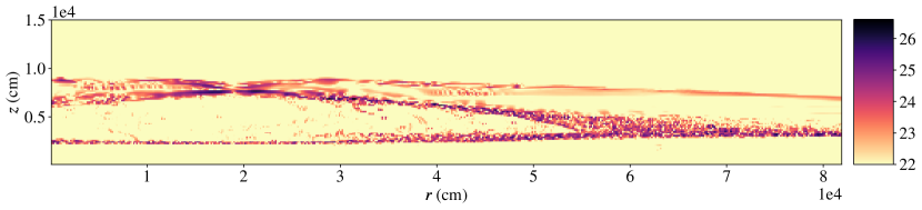
Figure 11: Baroclinicity. This plot shows $\ln\left(\mathbf{\psi}\right)$ at time $t=0.02~{}\mathrm{s}$ for the 10/10 simulation.

Vortical motions are also evident in a direct visualization of the velocity field, as seen in Figure 12. We observe turbulence in the wake of the flame and in the unburnt fuel ahead of the front, while a convective cycle sets up near the hottest part of the burning region. The cycle draws the cooler fluid near the interface into the center of the flame and drives hot ash out towards the instability at its surface, helping to facilitate the flame spreading. Convective mixing should still be important in 3D, but we would expect much more complicated flow patterns, with a greater contribution from small-scale features (Zingale et al., 2015).

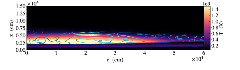
Figure 12: Streamlines showing velocity field at time $t=0.01~{}\mathrm{s}$ for the 10/10 simulation.

To further demonstrate the relationships between different properties of the flame, in Figure 13 we present some phase plots of the energy generation rate. The phase plot of the energy generation rate as a function of the $x$- and $y$-velocities shows that energy is preferentially generated in regions with negative $x$-velocity. This most likely corresponds to the burning along the underside of the flame front, where fuel has been entrained along the surface of the flame and so is moving in the opposite direction to the direction the flame is propagating in. This is further supported by the phase plot of the energy generation rate as a function of the $x$-velocity and the density, which shows that the energy generation rate peaks at $\rho\sim 3\times 10^{5}~{}\mathrm{g/cm}^{3}$, at the base of the flame. The energy generation rate also depends strongly on density.

In the first plot, there are “loops” of points of similar $\dot{e}_{\mathrm{nuc}}$ in the outer edges of the plot. These are likely to correspond to the vortices that appear within the flame, where the fluid moves in a circular motion in $u-v$ phase space.

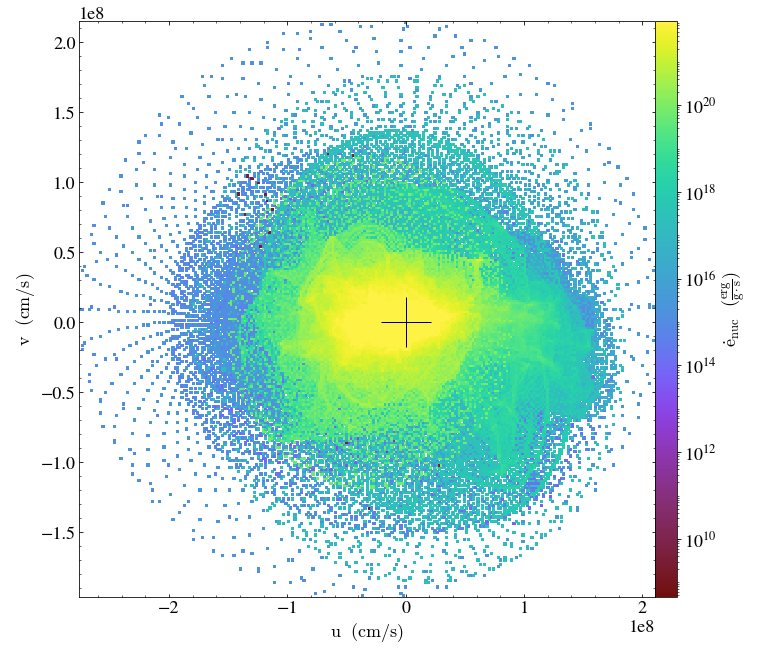
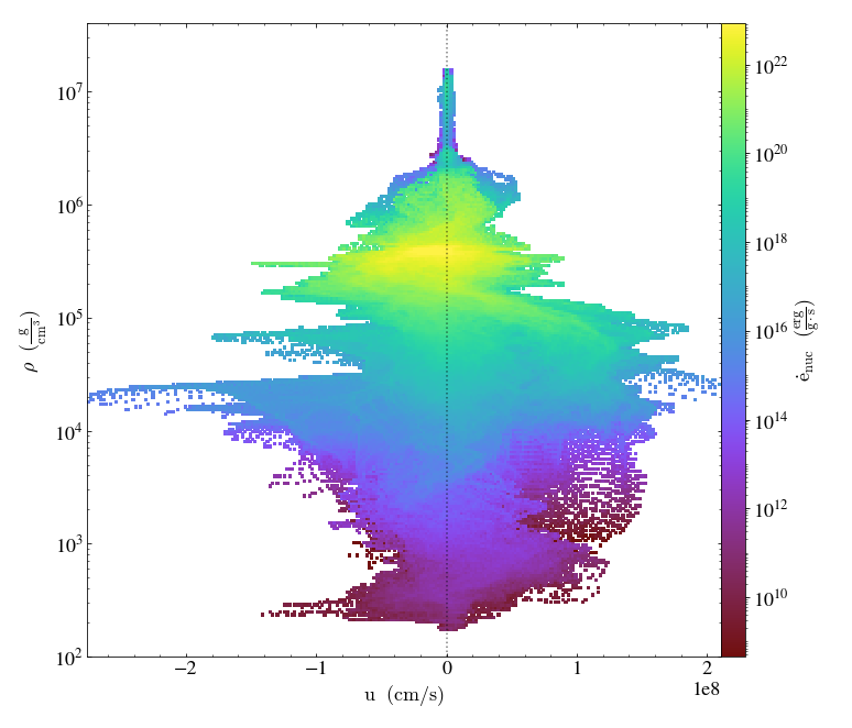
Figure 13: Phase plots at time $t=0.02~{}\mathrm{s}$. Left: Phase plot showing the energy generation rate as a function of the $x$- and $y$-velocities. The black cross shows the location of $u=v=0$. Right: phase plot showing the energy generation rate as a function of the $x$-velocity and the density.

Figure 14 shows the energy generation rate as a function of the temperature and $\bar{A}$. The energy generation rate peaks at low $\bar{A}$, where there is a high fraction of unburnt material. The burning raises the temperature of this material, such that the peak temperature coincides with the peak energy generation rate. The material then cools again as the burning converts the fuel into ashes, increasing $\bar{A}$ and reducing the energy generation rate as there is less available fuel. Along the base of the plot we see cool unburnt fluid and ashes. In the center of the plot there are thin ‘trails’ in phase space, which could correspond to less common reaction pathways in the reaction network.

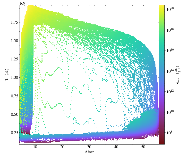
Figure 14: Phase plot of energy generation rate as a function of $\bar{A}$ and temperature at time $t=0.02~{}\mathrm{s}$.

6 Discussion

We have shown the results of our fully hydrodynamical, multidimensional simulations of flame propagation through the atmosphere of a neutron star. By using the fully compressible hydrodynamics equations, we are able to capture the vertical dynamics of the system. To accurately model the flame propagation, it is necessary to sufficiently resolve the scale height of the atmosphere. It is also important that there is a thin transition between the underlying neutron star and the atmosphere, to ensure that the peak temperature occurs at the correct base density.

In order to satisfy these requirements whilst allowing the simulations to be computationally feasible, we used several approximations: a higher than normal rotation rate, a boosted flame, a simplified reaction network, and a 2D axisymmetric model for the flow. The first two of these were used to reduce the model’s spatial and temporal scales. Using the simulation framework developed here, these both can be relaxed in the future, at the cost of more computer time. The same goes for 2D axisymmetry vs. full 3D—the only difference is computer time, and our future calculations will explore the 3D evolution and compare to the 2D simulations presented here. In particular, in 3D we will be able to explore shear instabilities at the flame front. We can also capture the baroclinic instability (Cavecchi & Spitkovsky, 2019) and the competition between it and shear. Larger networks are a straightforward change, and already supported in Castro using the pynucastro framework (Willcox & Zingale, 2018) and JINA ReacLib rate database (Cyburt et al., 2010b).

In addition to extending our models to 3D and relaxing the approximations used in this study, in the future we plan to perform a number of additional further studies. These include investigating the effects of ignition latitude and different initial models. We also plan to model mixed H/He bursts. This will require a different reaction network, and perhaps different resolution requirements. A long term goal is to include magnetohydrodynamics in our models. Although the magnetic fields of neutron stars exhibiting X-ray bursts are relatively weak, with $B\lesssim 10^{8}-10^{9}$G (Mukherjee et al., 2015) (at least compared to e.g. magnetars, which have $B\lesssim 10^{15}$G), it has been found by Cavecchi et al. (2016) that even weak magnetic fields could have a non-negligible effect on the flame propagation, reducing confinement due to the Coriolis force and leading to increased flame speeds. Ultimately, we wish to link our simulations to observed light curves. To do this, we will need to explore radiation transport in order to model how the burst energy propagates through the outer layers of the neutron star atmosphere.

In addition to exploring other aspects of the XRB physics, there are several changes to the algorithm used to model these XRBs we will pursue. First, as shown in Zingale et al. (2019), we have developed a fourth-order (in space and time) method for coupling hydrodynamics and reactions that should greatly improve the accuracy of the simulations. We expect that by using this new high-order algorithm we can drop a level of refinement from the simulations while still accurately modeling the evolution. We have also ported Castro to GPUs, giving an order of magnitude performance boost on nodes with both CPUs and GPUs. Flames without any boosting are currently running using the new GPU-enabled Castroand will be the focus of the next study.

Appendix A Diffusion Tests

To test our implementation of diffusion, we created a unit test in Castro that just uses the diffusion solver. This test uses the standard Gaussian initial conditions—the diffusion of a Gaussian remains Gaussian, with a lower amplitude and wider width. This is run with a constant diffusion coefficient. The point of this test is to demonstrate that the implementation done in a predictor-corrector form is second-order accurate.

We use a 2D axisymmetric geometry, with a reflection boundary on the symmetry axis (left) and Neumann boundaries on all other sides. In this geometry, the solution behaves like a spherical problem, and has the form:

$$T(r,t)=T_{1}+(T_{2}-T_{1})\left(\frac{t_{0}}{t+t_{0}}\right)^{3/2}e^{-r^{2}/(4D(t+t_{0}))}$$ (A1)

where $t_{0}$ is a small time used to set the initial width of the Gaussian, $r$ is the distance from the origin, and $D$ is the diffusion coefficient (see, e.g., Swesty & Myra (2009)). $T_{1}$ is the ambient temperature and $T_{2}$ is the temperature of the peak of the Gaussian. We use $D=1$, $T_{1}=1$, $T_{2}=2$, and $t_{0}=0.001$.

Table 5: Convergence of diffusion test problem.

base resolution	L-inf error	convergence rate
no refinement
32	5.995×10^-3	2.04
64	1.477×10^-3	2.01
128	3.664×10^-4	2.00
256	9.139×10^-5
one level of refinement
32	1.480×10^-3	2.01
64	3.685×10^-4	1.97
128	9.406×10^-5	1.94
256	2.446×10^-5

Table 5 shows the L-inf error against the analytic solution for the diffusion test problem. The tests were run in two fashions: no AMR, and AMR with one level of refinement (a jump of $2\times$). In both cases we see second-order convergence of the error. Figure 15 shows the temperature at the end of the simulation of the $64\times 128$ base grid plus one level of refinement simulation, with the grids shown to illustrate where the refinement jump is.

Figure 15: Temperature for the diffusion test problem at $10^{-3}~{}\mbox{s}$ for a diffusion test with a $64\times 128$ zone base grid and one level of refinement.

References

- Almgren et al. (2010) Almgren, A. S., Beckner, V. E., Bell, J. B., et al. 2010, ApJ, 715, 1221, doi: 10.1088/0004-637X/715/2/1221
- Bell et al. (2004) Bell, J. B., Day, M. S., Rendleman, C. A., Woosley, S. E., & Zingale, M. 2004, ApJ, 606, 1029, doi: 10.1086/383023
- Bhattacharyya & Strohmayer (2006) Bhattacharyya, S., & Strohmayer, T. E. 2006, 636, L121, doi: 10.1086/500199
- Bhattacharyya & Strohmayer (2007) —. 2007, 666, L85, doi: 10.1086/521790
- Brown et al. (1989) Brown, P. N., Byrne, G. D., & Hindmarsh, A. C. 1989, SIAM J. Sci. Stat. Comput., 10, 1038
- Cavecchi et al. (2016) Cavecchi, Y., Levin, Y., Watts, A. L., & Braithwaite, J. 2016, MNRAS, 459, 1259, doi: 10.1093/mnras/stw728
- Cavecchi & Spitkovsky (2019) Cavecchi, Y., & Spitkovsky, A. 2019, The Astrophysical Journal, 882, 142, doi: 10.3847/1538-4357/ab3650
- Cavecchi et al. (2013) Cavecchi, Y., Watts, A. L., Braithwaite, J., & Levin, Y. 2013, MNRAS, 434, 3526, doi: 10.1093/mnras/stt1273
- Cavecchi et al. (2015) Cavecchi, Y., Watts, A. L., Levin, Y., & Braithwaite, J. 2015, MNRAS, 448, 445, doi: 10.1093/mnras/stu2764
- Chakraborty & Bhattacharyya (2014) Chakraborty, M., & Bhattacharyya, S. 2014, ApJ, 792, 4, doi: 10.1088/0004-637X/792/1/4
- Colella & Woodward (1984) Colella, P., & Woodward, P. R. 1984, Journal of Computational Physics, 54, 174, doi: 10.1016/0021-9991(84)90143-8
- Cyburt et al. (2010a) Cyburt, R. H., Amthor, A. M., Ferguson, R., et al. 2010a, ApJS, 189, 240, doi: 10.1088/0067-0049/189/1/240
- Cyburt et al. (2010b) —. 2010b, ApJS, 189, 240, doi: 10.1088/0067-0049/189/1/240
- Fryxell & Woosley (1982) Fryxell, B. A., & Woosley, S. E. 1982, ApJ, 258, 733, doi: 10.1086/160121
- Galloway & Keek (2017) Galloway, D. K., & Keek, L. 2017, ArXiv e-prints. https://arxiv.org/abs/1712.06227
- Hunter (2007) Hunter, J. D. 2007, Computing in Science and Engg., 9, 90, doi: 10.1109/MCSE.2007.55
- Johnston et al. (2019) Johnston, Z., Heger, A., & Galloway, D. K. 2019, arXiv e-prints, arXiv:1909.07977. https://arxiv.org/abs/1909.07977
- José et al. (2010) José, J., Moreno, F., Parikh, A., & Iliadis, C. 2010, The Astrophysical Journal Supplement Series, 189, 204, doi: 10.1088/0067-0049/189/1/204
- Katz et al. (2016) Katz, M. P., Zingale, M., Calder, A. C., et al. 2016, ApJ, 819, 94, doi: 10.3847/0004-637X/819/2/94
- Khokhlov (1993) Khokhlov, A. 1993, ApJ, 419, L77, doi: 10.1086/187141
- Lampe et al. (2016) Lampe, N., Heger, A., & Galloway, D. K. 2016, The Astrophysical Journal, 819, doi: 10.3847/0004-637X/819/1/46
- Lin et al. (2006) Lin, D. J., Bayliss, A., & Taam, R. E. 2006, ApJ, 653, 545, doi: 10.1086/508863
- Malone et al. (2011) Malone, C. M., Nonaka, A., Almgren, A. S., Bell, J. B., & Zingale, M. 2011, ApJ, 728, 118, doi: 10.1088/0004-637X/728/2/118
- Malone et al. (2014) Malone, C. M., Nonaka, A., Woosley, S. E., et al. 2014, Astrophysical Journal, 782, 11, doi: 10.1088/0004-637X/782/1/11
- Malone et al. (2014) Malone, C. M., Zingale, M., Nonaka, A., Almgren, A. S., & Bell, J. B. 2014, ApJ, 788, 115, doi: 10.1088/0004-637X/788/2/115
- Miller & Colella (2002) Miller, G. H., & Colella, P. 2002, Journal of Computational Physics, 183, 26, doi: 10.1006/jcph.2002.7158
- Mukherjee et al. (2015) Mukherjee, D., Bult, P., van der Klis, M., & Bhattacharya, D. 2015, Monthly Notices of the Royal Astronomical Society, 452, 3994
- Nethercote & Seward (2007) Nethercote, N., & Seward, J. 2007, in Proceedings of the 28th ACM SIGPLAN Conference on Programming Language Design and Implementation, PLDI ’07 (New York, NY, USA: ACM), 89–100, doi: 10.1145/1250734.1250746
- Oliphant (2007) Oliphant, T. E. 2007, Computing in Science and Engg., 9, 10, doi: 10.1109/MCSE.2007.58
- O’Rourke & Bracco (1979) O’Rourke, P. J., & Bracco, F. V. 1979, Journal of Computational Physics, 33, 185
- Özel & Freire (2016) Özel, F., & Freire, P. 2016, Annual Review of Astronomy and Astrophysics, 54, 401
- Röpke et al. (2007) Röpke, F. K., Hillebrandt, W., Schmidt, W., et al. 2007, The Astrophysical Journal, 668, 1132, doi: 10.1086/521347
- Spitkovsky et al. (2002) Spitkovsky, A., Levin, Y., & Ushomirsky, G. 2002, ApJ, 566, 1018, doi: 10.1086/338040
- Steiner et al. (2010) Steiner, A. W., Lattimer, J. M., & Brown, E. F. 2010, Astrophysical Journal, 722, 33, doi: 10.1088/0004-637X/722/1/33
- Strang (1968) Strang, G. 1968, SIAM J. Numerical Analysis, 5, 506
- Swesty & Myra (2009) Swesty, F. D., & Myra, E. S. 2009, ApJS, 181, 1, doi: 10.1088/0067-0049/181/1/1
- the StarKiller Microphysics Development Team et al. (2019) the StarKiller Microphysics Development Team, Bishop, A., Fields, C. E., et al. 2019, starkiller-astro/Microphysics: 19.04, doi: 10.5281/zenodo.2620545
- Timmes (2000) Timmes, F. X. 2000, ApJ, 528, 913, doi: 10.1086/308203
- Timmes (2019) —. 2019
- Timmes et al. (2000) Timmes, F. X., Hoffman, R. D., & Woosley, S. E. 2000, The Astrophysical Journal Supplement Series, 129, 377, doi: 10.1086/313407
- Timmes & Swesty (2000) Timmes, F. X., & Swesty, F. D. 2000, ApJS, 126, 501, doi: 10.1086/313304
- Timmes & Woosley (1992) Timmes, F. X., & Woosley, S. E. 1992, ApJ, 396, 649, doi: 10.1086/171746
- Turk et al. (2011) Turk, M. J., Smith, B. D., Oishi, J. S., et al. 2011, ApJS, 192, 9, doi: 10.1088/0067-0049/192/1/9
- van der Walt et al. (2011) van der Walt, S., Colbert, S. C., & Varoquaux, G. 2011, Computing in Science & Engineering, 13, 22, doi: 10.1109/MCSE.2011.37
- Weinberg & Bildsten (2007) Weinberg, N. N., & Bildsten, L. 2007, The Astrophysical Journal, 670, 1291, doi: 10.1086/522111
- Weinberg et al. (2006) Weinberg, N. N., Bildsten, L., & Brown, E. F. 2006, The Astrophysical Journal, 650, L119, doi: 10.1086/508887
- Willcox & Zingale (2018) Willcox, D. E., & Zingale, M. 2018, Journal of Open Source Software, 3, 588, doi: 10.21105/joss.00588
- Woosley et al. (2004) Woosley, S. E., Heger, A., Cumming, A., et al. 2004, Astrophysical Journal Supplement, 151, 75, doi: 10.1086/381533
- Zhang et al. (2019) Zhang, W., Almgren, A., Beckner, V., et al. 2019, Journal of Open Source Software, 4, 1370, doi: 10.21105/joss.01370
- Zingale & Katz (2015) Zingale, M., & Katz, M. P. 2015, ApJS, 216, 31, doi: 10.1088/0067-0049/216/2/31
- Zingale et al. (2019) Zingale, M., Katz, M. P., Bell, J. B., et al. 2019, arXiv e-prints, arXiv:1908.03661. https://arxiv.org/abs/1908.03661
- Zingale et al. (2015) Zingale, M., Malone, C. M., Nonaka, A., Almgren, A. S., & Bell, J. B. 2015, ApJ, 807, 60, doi: 10.1088/0004-637X/807/1/60
- Zingale et al. (2001) Zingale, M., Timmes, F. X., Fryxell, B., et al. 2001, ApJS, 133, 195, doi: 10.1086/319182
- Zingale et al. (2002) Zingale, M., Dursi, L. J., ZuHone, J., et al. 2002, ApJS, 143, 539, doi: 10.1086/342754
- Zingale et al. (2017) Zingale, M., Almgren, A. S., Barrios Sazo, M. G., et al. 2017, ArXiv e-prints. https://arxiv.org/abs/1711.06203
- Zingale et al. (2018) Zingale, M., Almgren, A. S., Barrios Sazo, M. G., et al. 2018, in Journal of Physics Conference Series, Vol. 1031, Journal of Physics Conference Series, 012024, doi: 10.1088/1742-6596/1031/1/012024