1-Wasserstein Distance on the Standard Simplex

Abstract.

Wasserstein distances provide a metric on a space of probability measures. We consider the space $\Omega$ of all probability measures on the finite set $\chi=\{1,\dots,n\}$ where $n$ is a positive integer. 1-Wasserstein distance, $W_{1}(\mu,\nu)$ is a function from $\Omega\times\Omega$ to $[0,\infty)$. This paper derives closed form expressions for the First and Second moment of $W_{1}$ on $\Omega\times\Omega$ assuming a uniform distribution on $\Omega\times\Omega$.

1. Introduction

Wasserstein distances provide a natural metric on a space of probability measures. Intuitively, they measure the minimum amount of work required to transform one distribution into another. They have found application in numerous fields including computer vision [RTG00], statistics [PZ19], dynamical systems [Vil08], and many others.

Let $(\chi,d)$ be a Polish space and $\mu$ and $\nu$ be two probability measures on $\chi$. The p-Wasserstein distance between $\mu$ and $\nu$ is defined by:

$$W_{p}(\mu,\nu)=\bigg{(}\inf_{\pi\in\Pi(\mu,\nu)}\int_{\chi\times\chi}d(x,y)^{p}d\pi(x,y)\bigg{)}^{1/p},$$

where $\Pi(\mu,\nu)$ is the set of probability measures $\pi$ on $\chi\times\chi$ such that $\pi(A\times\chi)=\mu(A)$ and $\pi(\chi\times B)=\nu(B)$ for all measurable $A,B\subseteq\chi$. The measure $\pi$ with marginals $\mu$ and $\nu$ on the two components of $\chi\times\chi$ is called a coupling of $\mu$ and $\nu$.

In general,the Wasserstein distances do not admit closed form expressions. One important exception is the case where $\chi=\mathbb{R}$, $d(x,y)=|x-y|$, and $p=1$. In this case, we have the explicit formula [PZ19]:

$$W_{1}(\mu,\nu)=\int_{\mathbb{R}}|F_{\mu}(t)-F_{\nu}(t)|dt,$$

where $F_{\mu}(t)$ and $F_{\nu}(t)$ are the cumulative distribution functions of $\mu$ and $\nu$ respectively.

Here we specialize further, considering only $\chi=\{1,\dots,n\}$ where $n$ is a positive integer. Denote this finite set $[n]$. Let $\mu$ and $\nu$ be two probability measures on $[n]$. Then $W_{1}(\mu,\nu)$ reduces to $l_{1}$ distance between finite vectors:

(1) $$W_{1}(\mu,\nu)=\sum_{i=1}^{n}|F_{\mu}(i)-F_{\nu}(i)|=||F_{\mu}-F_{\nu}||_{1}.$$

There are numerous applications of Wasserstein distances on finite sets. In [BW19] Bourn and Willenbring, use $W_{1}$, which they refer to as Earth Movers Distance or EMD following computer science convention, to compare grade distributions - distributions on the finite set $\{A,A-,B+,\dots,F\}$. In that context, Bourn and Willenbring considered the space of all probability distributions on $[n]$, denoted $\mathcal{P}_{n}$ - the standard simplex or probability simplex. This space embeds naturally in $\mathbb{R}^{n}$, inherits Lebesgue measure, and has finite volume. A uniform probability measure is obtained by normalizing Lebesgue measure on $\mathcal{P}_{n}$ so that total mass of $\mathcal{P}_{n}$ is one. Similarly, $\mathcal{P}_{n}\times\mathcal{P}_{n}$ can be given a uniform product probability measure. Let $\mathcal{P}_{n}\times\mathcal{P}_{n}=\Omega_{n}$ with normalized Lebesgue measure be our probability space. Define the random variable $X_{n}(\mu,\nu)=W_{1}(\mu,\nu)$ on $\Omega_{n}$. What can we say about $X_{n}$?

The contribution of [BW19] to this question is the derivation of a recurrence $\mathcal{M}_{p,q}$ such that $\mathbb{E}(X_{n})=\mathcal{M}_{n,n}$. The recurrence is:

(2) $$\mathcal{M}_{p,q}=\frac{(p-1)\mathcal{M}_{p-1,q}+(q-1)\mathcal{M}_{p,q-1}+|p-q|}{p+q-1},$$

with $\mathcal{M}_{p,q}=0$ if either $p$ or $q$ is not positive. In this paper, we find a closed form for the first and second moment of $X_{n}$. Additionally, we “solve” the recurrence provided by [BW19] to verify consistency of results. This provides an interesting link between the discrete combinatorial approach of [BW19] and our calculus based approach.

The remainder of this paper is organized as follows. Section 2 presents our results and provides some discussion. Section 3 gives an overview of our approach to the problem. Section 4 proves the closed form for the first moment. Section 5 proves the closed form for the second moment. Section 6 solves the recurrence (2) of Bourn and Willenbring.

2. Main Result and Discussion

The main results of this paper are the following two theorems.

Theorem 1.

The first moment of $X_{n}$ is given by

$$\mathbb{E}(X_{n})=\frac{2^{2n-3}(n-1)}{(2n-1)!}(n-1)!^{2}.$$

Theorem 2.

The second moment of $X_{n}$ is given by

$$\mathbb{E}(X_{n}^{2})=\frac{(n-1)(7n-4)}{30n}.$$

2.1. Unit Normalized $W_{1}$

[BW19] defines unit normalized EMD on $\mathcal{P}_{n}$ as EMD scaled by $\frac{1}{n-1}$ - this is $W_{1}(\mu,\nu)\frac{1}{n-1}$. We will refer to this as unit normalized $W_{1}$ or $\widetilde{W_{1}}$. This makes $P_{n}$ into a metric space with diameter one. Intuitively, $W_{1}$ places the finite set $[n]$ on the first $n$ positive integers of the real number line, while $\widetilde{W_{1}}$ partitions the unit interval $[0,1]$ with $n$ equally spaced points. $W_{1}$ has a constant distance of one between adjacent points. $\widetilde{W_{1}}$ has constant maximum distance (diameter) of one. If we define $\widetilde{X_{n}}=\frac{X_{n}}{n-1}$, we can write closed forms for the first and second moment of unit normalized $W_{1}$ on $\Omega$:

$$\mathbb{E}(\widetilde{X_{n}})=\frac{2^{2n-3}(n-1)!^{2}}{(2n-1)!}.$$

$$\mathbb{E}(\widetilde{X_{n}^{2}})=\frac{(7n-4)}{30n(n-1)}.$$

2.2. Asymptotic Behavior

We briefly consider the asymptotic behavior of the first and second moment. The table below presents approximate numeric values for the first and second moment, and the variance, for $X_{n}$ and $\widetilde{X_{n}}$.

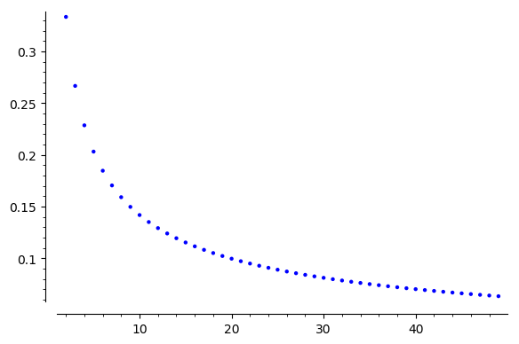
Figure 1. $\mathbb{E}(\widetilde{X_{n}})$ for n=2 to 50

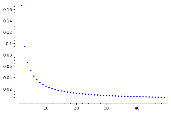
Figure 2. $\mathbb{E}(\widetilde{X_{n}^{2}})$ for n=2 to 50

$n$	$\mathbb{E}(X_{n})$	$\mathbb{E}(X_{n}^{2})$	$\text{Var}(X_{n})$	$\mathbb{E}(\widetilde{X_{n}})$	$\mathbb{E}(\widetilde{X_{n}^{2}})$	$\text{Var}(\widetilde{X_{n}})$
$2$	$0.3333$	$0.1667$	$0.05556$	$0.3333$	$0.1667$	$0.05556$
$3$	$0.5333$	$0.3778$	$0.09333$	$0.2667$	$0.09444$	$0.02333$
$4$	$0.6857$	$0.6000$	$0.1298$	$0.2286$	$0.06667$	$0.01442$
$5$	$0.8127$	$0.8267$	$0.1662$	$0.2032$	$0.05167$	$0.01039$
$6$	$0.9235$	$1.056$	$0.2027$	$0.1847$	$0.04222$	$0.008107$
$7$	$1.023$	$1.286$	$0.2392$	$0.1705$	$0.03571$	$0.006645$
$8$	$1.114$	$1.517$	$0.2759$	$0.1591$	$0.03095$	$0.005630$
$9$	$1.198$	$1.748$	$0.3126$	$0.1498$	$0.02731$	$0.004884$
$10$	$1.277$	$1.980$	$0.3493$	$0.1419$	$0.02444$	$0.004313$

Now we consider the behavior of $\mathbb{E}(X_{n})$ and $E(\widetilde{X_{n}})$ as $n\to\infty$. As discussed above:

$$\mathbb{E}(X_{n})=\frac{2^{2n-3}(n-1)}{(2n-1)!}(n-1)!^{2}.$$

We can rewrite this in the form:

$$\mathbb{E}(X_{n})=4^{n-1}\frac{(n-1)}{n}\frac{1}{\binom{2n}{n}}.$$

It is known that [Cam94]

$$\binom{2n}{n}\sim\frac{4^{n}}{\sqrt{\pi n}}.$$

The symbol $\sim$ means the quotient of the left and right side converges to 1 as $n\to\infty$. Therefore,

$$\mathbb{E}(X_{n})\sim\frac{\sqrt{\pi n}}{4}.$$

Dividing through by $n-1$,

$$\mathbb{E}(\widetilde{X_{n}})\sim\frac{1}{4}\sqrt{\frac{\pi}{n}}.$$

We also have:

$$\mathbb{E}(X_{n}^{2})=\frac{(n-1)(7n-4)}{30n}$$

$$\mathbb{E}(\widetilde{X_{n}^{2}})=\frac{(7n-4)}{30n(n-1)}.$$

Therefore, for the variance we obtain:

$$\text{Var}(X_{n})=\mathbb{E}(X_{n}^{2})-\mathbb{E}(X_{n})^{2}\sim\bigg{(}\frac{7}{30}-\frac{\pi}{16}\bigg{)}n$$

$$\text{Var}(\widetilde{X_{n}})=\mathbb{E}(\widetilde{X_{n}^{2}})-\mathbb{E}(\widetilde{X_{n}})^{2}\sim\bigg{(}\frac{7}{30}-\frac{\pi}{16}\bigg{)}\frac{1}{n}.$$

2.3. Probability Measures for $X_{n}$

It would be nice to have explicit probability measures for $X_{n}$. Toward this end, we computed the probability density functions for $X_{2}$, $X_{3}$ as:

$$p_{X_{2}}(t)=2-2t$$

$$p_{X_{3}}(t)=\begin{cases}\frac{19}{2}t^{4}-\frac{14}{3}t^{3}+4t^{2}&\text{if $0\leq t\leq 1$}\\ -\frac{1}{12}t^{4}+\frac{2}{3}t^{3}-2t^{2}+\frac{8}{3}t-\frac{1}{3}&\text{if $1<t\leq 2$}\end{cases}$$

Further work could be done to determine probability measures for $n>3$.

Figure 3. Probability Density Function $p_{X_{3}}(t)$

3. Approach

We have the probability space $(\Omega_{n},\mathcal{B}(\Omega_{n}),\phi)$ where $\mathcal{B}(\Omega_{n})$ denotes the Borel $\sigma$-algebra on $\Omega_{n}$ and $\phi$ is Lebesgue measure normalized such that $\phi(\Omega_{n})=1$. Our random variable is $X_{n}(\mu,\nu)=W_{1}(\mu,\nu)$. It is easy to write the first and second moment of $X_{n}$ as integrals over $\Omega_{n}$. The first moment is given by:

$$\mathbb{E}(X_{n})=\int_{\Omega_{n}}X_{n}(\mu,\nu)d\phi.$$

The second moment is given by:

$$\mathbb{E}(X_{n}^{2})=\int_{\Omega_{n}}X_{n}^{2}(\mu,\nu)d\phi.$$

For computation, we work with the closed form (1). Let $\mathcal{C}_{n}$ be the space of cumulative distributions on $[n]$. Consider the probability space $(U_{n},\mathcal{B}(U_{n}),\phi)$, where $U_{n}=\mathcal{C}_{n}\times\mathcal{C}_{n}$, $\mathcal{B}(U_{n})$ denotes the Borel $\sigma$-algebra on $U_{n}$, and $\phi$ is Lebesgue measure normalized such that $\phi(U_{n})=1$. Define the random variable $Y_{n}(F_{\mu},F_{\nu})=||F_{\mu}-F_{\nu}||_{1}$ on $U_{n}$. The transformation $T:\mathcal{P}_{n}\to\mathcal{C}_{n}$ is volume preserving. By this fact and (1), we conclude $\mathbb{E}(X_{n})=\mathbb{E}(Y_{n})$ and $\mathbb{E}(X_{n}^{2})=\mathbb{E}(Y_{n}^{2})$. Section 4 proves Theorem 1 from the integral:

$$\mathbb{E}(Y_{n})=\int_{U_{n}}Y_{n}(F_{\mu},F_{\nu})d\phi.$$

Section 5 proves Theorem 2 from the integral:

$$\mathbb{E}(Y_{n}^{2})=\int_{U_{n}}Y_{n}^{2}(F_{\mu},F_{\nu})d\phi.$$

To find the closed forms presented in Theorem 1 and Theorem 2, we are led to the evaluation of certain sums for which [PWZ96] is a general reference.

4. Proof of Theorem 1

The space of all cumulative distributions on $[n]$ is given by

$$\mathcal{C}_{n}=\{(x_{1},...,x_{n})\,|\,0\leq x_{1}\leq...\leq x_{n}=1\}.$$

$\mathcal{C}_{n}$ is a simplex contained in the hyperplane $x_{n}=1$ and thus embeds naturally in $\mathbb{R}^{n-1}$. Henceforth, we will think of $\mathcal{C}_{n}$ as embedded in $\mathbb{R}^{n-1}$. For $t\geq 0$, $n\in\mathbb{N},$ and $n\geq 2$, let $\mathcal{C}_{n}(t)$ be the set:

$$\mathcal{C}_{n}(t)=\{(x_{1},x_{2},\dots,x_{n-1})\in\mathbb{R}^{n-1}:0\leq x_{1}\leq x_{2}\leq\dots\leq x_{n-1}\leq t\}.$$

Let $s,t\geq 0$, $\textbf{x}\in\mathcal{C}_{n}(t)$, $\textbf{y}\in\mathcal{C}_{n}(s)$ and set

$$\mathcal{V}_{n}(s,t) = \int_{\mathcal{C}_{n}(s)}\int_{\mathcal{C}_{n}(t)}1\,d\textbf{x}\,d\textbf{y}=\frac{s^{n-1}t^{n-1}}{(n-1)!^{2}},$$

$$\mathcal{F}_{n}(s,t) = \int_{\mathcal{C}_{n}(s)}\int_{\mathcal{C}_{n}(t)}\|\textbf{x}-\textbf{y}\|_{1}d\textbf{x}\,d\textbf{y}.$$

Then,

$$\mathbb{E}(Y_{n})=\frac{\mathcal{F}_{n}(1,1)}{\mathcal{V}_{n}(1,1)}.$$

If we set $\mathcal{F}_{1}(s,t)=0$, then the functions $\mathcal{F}_{n}$ are determined recursively by

$$\mathcal{F}_{n}(s,t)=\int_{0}^{t}\int_{0}^{s}(\mathcal{F}_{n-1}(x,y)+|x-y|\mathcal{V}_{n-1}(x,y))\,dx\,dy.$$

Here $x=x_{n-1}$ and $y=y_{n-1}$ are the last components of $\mathcal{C}_{n}(t)$ and $\mathcal{C}_{n}(s)$ respectively. Fubini’s theorem is relied on to justify evaluating $\mathcal{F}_{n}(s,t)$ as an iterated integral.

This recursion formula is awkward to use because of the appearance of the absolute value $|x-y|$. We remove this absolute value as follows. The function $\mathcal{F}_{n}(s,t)$ is symmetric in $(s,t)$. Therefore, it is sufficient to consider $s\geq t$ which we will always assume. Introduce the integral operator

$$(If)(s,t)=2\int_{0}^{t}\int_{y}^{t}f(x,y)\,dx\,dy+\int_{0}^{t}\int_{t}^{s}f(x,y)\,dx\,dy.$$

Then, for $0\leq t\leq s$,

(3) $$\mathcal{F}_{n}(s,t)=I\left(\mathcal{F}_{n-1}(x,y)+(x-y)\mathcal{V}_{n-1}(x,y)\right).$$

This is a recursion formula for $\mathcal{F}_{n}(s,t)$ in the region $0\leq t\leq s$. We note that, for $i,j=0,1,2,\dots$,

(4) $$I(x^{i}y^{j})=\frac{s^{i+1}t^{j+1}}{(i+1)(j+1)}+\frac{(i-j)t^{i+j+2}}{(i+1)(j+1)(i+j+2)}.$$

It follows from (3) and (4) that $\mathcal{F}_{n}(s,t)$ is a polynomial in $s,t$ of the form

(5) $$\mathcal{F}_{n}(s,t)=\sum_{k=0}^{n}f_{n,k}t^{n+k-1}s^{n-k}.$$

For example, we get

$$\mathcal{F}_{2}(s,t) = \frac{ts^{2}}{2}-\frac{t^{2}s}{2}+\frac{t^{3}}{3},$$

$$\mathcal{F}_{3}(s,t) = \frac{t^{2}s^{3}}{4}-\frac{t^{3}s^{2}}{4}+\frac{t^{4}s}{12}+\frac{t^{5}}{20},$$

$$\mathcal{F}_{4}(s,t) = \frac{t^{3}s^{4}}{24}-\frac{t^{4}s^{3}}{24}+\frac{t^{5}s^{2}}{120}+\frac{t^{6}s}{120}+\frac{t^{7}}{420},$$

$$\mathcal{F}_{5}(s,t) = \frac{t^{4}s^{5}}{288}-\frac{t^{5}s^{4}}{288}+\frac{t^{6}s^{3}}{2160}+\frac{{t}^{7}{s}^{2}}{1680}+\frac{t^{8}s}{3360}+\frac{t^{9}}{18144}.$$

Using (3) and (4), we find

$$f_{n,0}=\frac{f_{n-1,0}}{n(n-1)}+\frac{1}{n(n-1)(n-2)!^{2}}\quad\text{for $n\geq 2$}.$$

We set

$$\tilde{f}_{n,k}=f_{n,k}(n+k-1)!(n-k)!$$

Then

$$\tilde{f}_{n,0}-\tilde{f}_{n-1,0}=n-1.$$

Since $f_{1,0}=0$ we find $\tilde{f}_{n,0}=\frac{1}{2}n(n-1)$ so

(6) $$f_{n,0}=\frac{n(n-1)}{2(n-1)!n!}=\frac{1}{2(n-1)!(n-2)!}.$$

Similarly, we obtain

(7) $$f_{n,1}=-f_{n,0}=-\frac{1}{2(n-1)!(n-2)!}.$$

Now (3) and (4) give

$$f_{n,k}=\frac{f_{n-1,k}}{(n+k-1)(n-k)}\quad\text{for $2\leq k<n$.}$$

Therefore,

$$\tilde{f}_{n,k}=\tilde{f}_{n-1,k}\quad\text{for $2\leq k<n$}$$

and

(8) $$f_{n,k}=\frac{f_{k,k}(2k-1)!}{(n+k-1)!(n-k)!}\quad\text{for $2\leq k\leq n$.}$$

Using again (3) and (4) we obtain

(9) $$f_{n,n}=\sum_{k=0}^{n-1}\frac{f_{n-1,k}(1-2k)}{(n+k-1)(n-k)(2n-1)}+\frac{2}{n!(n-2)!(2n-1)}.$$

In (9) we substitute (6), (7), (8) and find

(10) $$f_{n,n}=\sum_{k=2}^{n-1}\frac{f_{k,k}(2k-1)!(1-2k)}{(n+k-1)!(n-k)!(2n-1)}+\frac{1}{(n-1)!(n-2)!(2n-1)}.$$

This is a recursion formula for the “diagonal sequence” $f_{k,k}$. With the help of a computer we guess the solution

(11) $$f_{k,k}=\frac{(k-1)k}{(2k-1)!}.$$

We prove (11) by induction on $k$. The formula is true for $k=1$. Suppose (11) holds for all $k$ less than a given $n\geq 2$. Then we substitute $f_{k,k}$ given by (11) on the right-hand side of (10). Since (see Appendix A)

$$\sum_{k=2}^{n}\frac{k(k-1)(2k-1)}{(n+k-1)!(n-k)!}=2A_{n,3}-3A_{n,2}+A_{n,1}=\frac{1}{(n-1)!(n-2)!}$$

we obtain (11) for $k=n$. This completes the inductive proof of (11).

Now (8), (11) give

(12) $$f_{n,k}=\frac{(k-1)k}{(n+k-1)!(n-k)!}\quad\text{for $2\leq k\leq n$}.$$

In particular, using again Appendix A, we have

$$\mathcal{F}_{n}(1,1) = \sum_{k=0}^{n}f_{n,k}=\sum_{k=2}^{n}f_{n,k}$$

$$= \sum_{k=2}^{n}\frac{(k-1)k}{(n+k-1)!(n-k)!}$$

$$= A_{n,2}-A_{n,1}$$

$$= \frac{2^{2n-3}(n-1)}{(2n-1)!}.$$

Thus,

$$\mathbb{E}(X_{n})=\mathbb{E}(Y_{n})=\frac{\mathcal{F}_{n}(1,1)}{\mathcal{V}_{n}(1,1)}=\frac{2^{2n-3}(n-1)}{(2n-1)!}(n-1)!^{2}.$$

5. Proof of Theorem 2

Let $s,t\geq 0$, $\textbf{x}\in\mathcal{C}_{n}(t)$, $\textbf{y}\in\mathcal{C}_{n}(s)$ and define

$$\mathcal{G}_{n}(s,t)=\int_{\mathcal{C}_{n}(s)}\int_{\mathcal{C}_{n}(t)}\|\textbf{x}-\textbf{y}\|_{1}^{2}d\textbf{x}\,d\textbf{y}.$$

If we set $\mathcal{G}_{1}(s,t)=0$ then the function $\mathcal{G}_{n}$ is determined recursively by

$$\mathcal{G}_{n}(s,t)=\int_{0}^{t}\int_{0}^{s}(\mathcal{G}_{n-1}(x,y)+2|x-y|\mathcal{F}_{n-1}(x,y)+(x-y)^{2}\mathcal{V}_{n-1}(x,y))\,dx\,dy.$$

As in the proof of Theorem 1, $x=x_{n-1}$, $y=y_{n-1}$ and Fubini’s theorem justifies evaluating $\mathcal{G}_{n}(s,t)$ as an iterated integral.

The function $\mathcal{G}_{n}(s,t)$ is symmetric in $(s,t)$. Therefore, it is sufficient to consider $s\geq t$. Then, for $0\leq t\leq s$,

(13) $$\mathcal{G}_{n}(s,t)=I\left(\mathcal{G}_{n-1}(x,y)+2(x-y)\mathcal{F}_{n-1}(x,y)+(x-y)^{2}\mathcal{V}_{n-1}(x,y)\right).$$

This is a recursion formula for $\mathcal{G}_{n}(s,t)$ in the region $0\leq t\leq s$. It follows from (13) and (4) that $\mathcal{G}_{n}(s,t)$ is a polynomial in $s,t$ of the form

(14) $$\mathcal{G}_{n}(s,t)=\sum_{k=-1}^{n}g_{n,k}t^{n+k}s^{n-k}.$$

For example,

$$\mathcal{G}_{2}(s,t) = \frac{ts^{3}}{3}-\frac{t^{2}s^{2}}{2}+\frac{t^{3}s}{3},$$

$$\mathcal{G}_{3}(s,t) = \frac{7t^{2}s^{4}}{24}-\frac{t^{3}s^{3}}{2}+\frac{3t^{4}s^{2}}{8}-\frac{2t^{5}s}{15}+\frac{11t^{6}}{180},$$

$$\mathcal{G}_{4}(s,t) = \frac{5t^{3}s^{5}}{72}-\frac{t^{4}s^{4}}{8}+\frac{31t^{5}s^{3}}{360}-\frac{t^{6}s^{2}}{60}-\frac{t^{7}s}{180}+\frac{t^{8}}{120},$$

$$\mathcal{G}_{5}(s,t) = \frac{13t^{4}s^{6}}{1728}-\frac{t^{5}s^{5}}{72}+\frac{77t^{6}s^{4}}{8640}-\frac{t^{7}s^{3}}{1260}-\frac{11t^{8}s^{2}}{10080}+\frac{t^{9}s}{2520}+\frac{19t^{10}}{50400}.$$

First we determine $g_{n,k}$ for $k=-1$. From (13) and (4) we obtain

$$g_{n,-1}=\frac{g_{n-1,-1}}{(n-1)(n+1)}+\frac{2f_{n-1,0}}{(n-1)(n+1)}+\frac{1}{(n-2)!^{2}(n-1)(n+1)}.$$

Using (6) this yields

$$g_{n,-1}=\frac{g_{n-1,-1}}{(n-1)(n+1)}+\frac{1}{(n-1)!(n-3)!(n+1)}+\frac{1}{(n-2)!^{2}(n-1)(n+1)}.$$

Let

$$g_{n,k}=\frac{\tilde{g}_{n,k}}{(n-k)!(n+k)!}.$$

Then

$$\tilde{g}_{n,-1}-\tilde{g}_{n-1,-1}=(n-1)^{2}n.$$

This gives

$$\tilde{g}_{n,-1}=\tilde{g}_{1,-1}+\sum_{m=2}^{n}(m-1)^{2}m=\frac{1}{12}n(n-1)(3n-2)(n+1).$$

Therefore,

(15) $$g_{n,-1}=\frac{n(n-1)(3n-2)(n+1)}{12(n-1)!(n+1)!}=\frac{n(3n-2)}{12(n-2)!n!}.$$

From (13) and (4) we obtain the recursion formula

$$g_{n,0}=\frac{g_{n-1,0}}{n^{2}}+\frac{2f_{n-1,1}-2f_{n-1,0}}{n^{2}}-\frac{2}{n^{2}(n-2)!^{2}}.$$

This gives

$$\tilde{g}_{n,0}-\tilde{g}_{n-1,0}=-2(n-1)^{3}$$

and

(16) $$g_{n,0}=-\frac{1}{2(n-2)!^{2}}.$$

From (13) and (4) we obtain the recursion formula

$$g_{n,1}=\frac{g_{n-1,1}}{(n-1)(n+1)}+\frac{2f_{n-1,2}-2f_{n-1,1}}{(n-1)(n+1)}+\frac{1}{(n-2)!^{2}(n-1)(n+1)}.$$

This gives

$$\tilde{g}_{n,1}-\tilde{g}_{n-1,1}=4(n-2)+n(n-1)^{2}$$

and

(17) $$g_{n,1}=\frac{2(n-1)(n-2)}{(n-1)!(n+1)!}+\frac{n(n-1)(3n-2)(n+1)}{12(n-1)!(n+1)!}.$$

Now let $k\geq 2$. Then (13) and (4) give

$$g_{n,k}=\frac{g_{n-1,k}}{(n+k)(n-k)}+\frac{2f_{n-1,k+1}-2f_{n-1,k}}{(n+k)(n-k)}.$$

This leads to the recursion formula

$$\tilde{g}_{n,k}-\tilde{g}_{n-1,k}=4k(n-k^{2}-1)\quad\text{for $2\leq k<n$}.$$

This gives

(18) $$\tilde{g}_{n,k}=\tilde{g}_{k,k}+2k(k-n)(2k^{2}-k-n+1).$$

From (13) and (4) we find

(19) $$g_{n,n}=-\sum_{k=-1}^{n-1}\frac{kg_{n-1,k}}{(n-k)(n+k)n}-\sum_{k=1}^{n-2}\frac{2kf_{n-1,k+1}}{(n-k)(n+k)n}+\sum_{k=2}^{n-1}\frac{2kf_{n-1,k}}{(n-k)(n+k)n}.$$

It should be noted that the term $(x-y)^{2}\mathcal{V}_{n-1}(x,y)$ in (13) does not contribute to this formula because it is a symmetric polynomial. Using (12) and Appendix A we evaluate the second and third sum on the right-hand side of (19). We find

$$-\sum_{k=1}^{n-2}\frac{2kf_{n-1,k+1}}{(n-k)(n+k)n} = \frac{4^{n-1}(n+1)}{(2n)!}-\frac{n(n-2)}{n!^{2}}-\frac{n+1}{(2n-1)!},$$

$$\sum_{k=2}^{n-1}\frac{2kf_{n-1,k}}{(n-k)(n+k)n} = \frac{4^{n-1}(n+1)}{(2n)!}+\frac{n(n-2)}{n!^{2}}-\frac{1}{2(2n-3)!}.$$

Therefore, (19) can be written as

(20) $$g_{n,n}=-\sum_{k=-1}^{n-1}\frac{kg_{n-1,k}}{(n-k)(n+k)n}+\frac{2^{2n-1}(n+1)}{(2n)!}-\frac{2(n^{2}-n+1)}{(2n-1)!}.$$

Using (15), (17) we find that

(21) $$-\sum_{k=-1}^{1}\frac{kg_{n-1,k}}{(n-k)(n+k)n}=-\frac{2(n-3)(n-2)}{n!^{2}(n+1)}.$$

We also have

(22) $$-\sum_{k=2}^{n-1}\frac{2k^{2}(k-n+1)(2k^{2}-k-n+2)}{n(n-k)!(n+k)!}$$

$$=\frac{4^{n-1}(n+1)(4n-3)}{(2n)!}+\frac{2(n^{2}-n+1)}{(2n-1)!}-\frac{4n^{3}+n^{2}+9n-12}{(n+1)n!^{2}}.$$

We now substitute (18), (21), (22) in (20) and obtain

(23) $$g_{n,n}=-\sum_{k=2}^{n-1}\frac{k(2k)!g_{k,k}}{(n-k)!(n+k)!n}+\frac{4^{n-1}(n+1)(4n-1)}{(2n)!}-\frac{4n-1}{n(n-1)!^{2}}.$$

This is a recursion formula for the sequence $g_{n,n}$. With the help of a computer we guess

(24) $$g_{k,k}=\frac{(k-2)(4k-1)}{30(2k-3)!}\quad\text{for $k\geq 2$}.$$

We prove (24) by induction on $k$. This equation is true for $k=2$. Suppose it is true for all $k$ less than a given $n\geq 3$. Then we use (24) in (23). Using Appendix A, we evaluate the sum and and obtain the correct expression for $g_{n,n}$. The inductive proof is complete.

From (18) we get, for $2\leq k\leq n$,

(25) $$g_{n,k}=\frac{k(2k-1)(2k-2)(k-2)(4k-1)}{15(n+k)!(n-k)!}+\frac{2k(k-n)(2k^{2}-k-n+1)}{(n+k)!(n-k)!}.$$

In particular, we have

$$\mathcal{G}_{n}(1,1)=\sum_{k=-1}^{n}g_{n,k}=\frac{n(n-1)(7n-4)}{30n!^{2}}.$$

Thus,

$$\mathbb{E}(X_{n}^{2})=\mathbb{E}(Y_{n}^{2})=\frac{\mathcal{G}_{n}(1,1)}{\mathcal{V}_{n}(1,1)}=\frac{(n-1)(7n-4)}{30n}.$$

6. Solution to [BW19] Recurrence

In [BW19] a double sequence $\mathcal{M}_{p,q}$, $p,q\in\mathbb{N}_{0}$, is defined as the solution of the recursion (2). Here we “solve” this recursion.

In order to simplify the recursion we set

$$\mathcal{L}_{p,q}=\frac{(p+q-1)!}{(p-1)!(q-1)!}\mathcal{M}_{p,q},\quad\text{$p,q\in\mathbb{N}$,}$$

and $\mathcal{L}_{p,0}=\mathcal{L}_{0,q}=0$. Then (2) becomes

(26) $$\mathcal{L}_{p,q}=\mathcal{L}_{p-1,q}+\mathcal{L}_{p,q-1}+|p-q|\binom{p+q-2}{p-1},\quad\text{$p,q\in\mathbb{N}$}.$$

Note that $\mathcal{L}_{p,q}$ is a nonnegative integer for all $p,q$. The matrix $\mathcal{L}_{p,q}$, $p,q=0,\dots,6$, is

$$\begin{pmatrix}0&0&0&0&0&0&0\\ 0&0&1&3&6&10&15\\ 0&1&2&8&22&47&86\\ 0&3&8&16&48&125&274\\ 0&6&22&48&96&256&642\\ 0&10&47&125&256&512&1280\\ 0&15&86&274&642&1280&2560\end{pmatrix}$$

Consider the more general recursion

(27) $$\mathcal{K}_{p,q}=\mathcal{K}_{p-1,q}+\mathcal{K}_{p,q-1}+a_{p,q},\quad p,q\in\mathbb{N},$$

with initial condition $\mathcal{K}_{p,0}=\mathcal{K}_{0,q}=0$, where $\{a_{p,q}\}$ is a given double sequence. As a special case consider $a_{p,q}=1$ if $p=i$, $q=j$ for some given $i,j\in\mathbb{N}$, and $a_{p,q}=0$ otherwise. If $p\geq i$, $q\geq j$ the corresponding solution is

$$\mathcal{K}_{p,q}=\binom{p+q-i-j}{p-i}.$$

Therefore, by superposition, the solution of (26) is

$$\mathcal{L}_{p,q}=\sum_{i=1}^{p}\sum_{j=1}^{q}|i-j|\binom{i+j-2}{i-1}\binom{p+q-i-j}{p-i}.$$

We rewrite this in the slightly nicer form

(28) $$\mathcal{L}_{p+1,q+1}=\sum_{i=0}^{p}\sum_{j=0}^{q}|i-j|\binom{i+j}{i}\binom{p+q-i-j}{p-i}.$$

In a sense we found the solution of (26) and so also of (2). However, the question arises whether we can express the double sum in (28) (more) explicitly. We evaluate the double sum in (28) when $p=q$. There is some evidence (from the computer) that this is not possible when $p\neq q$. We could handle some special case like small $p$ or small $|p-q|$.

We now evaluate the double sum in (28) when $p=q$. First, we introduce $i+j=m$ as a new summation index. Then

$$\mathcal{L}_{p+1,p+1}=\sum_{m=0}^{2p}\sum_{i=0}^{p}|m-2i|\binom{m}{i}\binom{2p-m}{p-i},$$

where we use the standard convention that $\binom{n}{k}=0$ unless $0\leq k\leq n$. We remove the absolute value by writing

(29) $$\mathcal{L}_{p+1,p+1}=2\sum_{m=0}^{2p}\sum_{i=0}^{\lfloor m/2\rfloor}(m-2i)\binom{m}{i}\binom{2p-m}{p-i}.$$

The inside sum can be evaluated as a telescoping sum as follows. Consider first an even $m=2r$. Then

$$\sum_{i=0}^{r}2(r-i)\binom{2r}{i}\binom{2p-2r}{p-i}=\sum_{j=0}^{r}2j\binom{2r}{r-j}\binom{2s}{s+j},$$

where we set $i=r-j$ and $s=p-r$. Note that $\binom{2r}{r-j}=\binom{2r}{r+j}$. Now

$$2j\binom{2r}{r-j}\binom{2s}{s+j}=d_{j}-d_{j+1},\quad j=0,1,\dots,r,$$

where

$$d_{j}=\frac{(r+j)(s+j)}{r+s}\binom{2r}{r-j}\binom{2s}{s+j}.$$

Note that $d_{r+1}=0$. Therefore,

$$\sum_{i=0}^{r}2(r-i)\binom{2r}{i}\binom{2p-2r}{p-i}=d_{0}-d_{r+1}=d_{0}=\frac{rs}{r+s}\binom{2r}{r}\binom{2s}{s}.$$

If $m=2r+1$ is odd, we use

$$(2j+1)\binom{2r+1}{r-j}\binom{2s-1}{s+j}=e_{j}-e_{j+1},$$

where

$$e_{j}=\frac{(r+1+j)(s+j)}{r+s}\binom{2r+1}{r-j}\binom{2s-1}{s+j}.$$

Therefore,

$$\sum_{i=0}^{r}(2r+1-2i)\binom{2r+1}{i}\binom{2p-2r-1}{p-i}=e_{0}=\frac{(r+1)s}{r+s}\binom{2r+1}{r}\binom{2s-1}{s-1}.$$

Substituting these results in (29) we obtain

(30) $$\mathcal{L}_{p+1,p+1}=\sum_{r=0}^{p}\frac{2r(p-r)}{p}\binom{2r}{r}\binom{2p-2r}{p-r}+\sum_{r=0}^{p-1}\frac{2(r+1)(p-r)}{p}\binom{2r+1}{r}\binom{2p-2r-1}{p-r-1}.$$

The sums appearing in (30) are easy to evaluate. We note that

$$(1-4x)^{-1/2}=\sum_{n=0}^{\infty}\binom{2n}{n}x^{n}\quad\text{for $|x|<\frac{1}{4}$},$$

so

$$2x(1-4x)^{-3/2}=\sum_{n=0}^{\infty}n\binom{2n}{n}x^{n}.$$

If we compare coefficients in

$$\frac{2x}{(1-4x)^{3/2}}\frac{2x}{(1-4x)^{3/2}}=\frac{4x^{2}}{(1-4x)^{3}}=\sum_{n=0}^{\infty}2^{2n-3}n(n-1)x^{n}$$

we find the first sum in (30). Using $\binom{2r+1}{r}=\frac{1}{2}\binom{2r+2}{r+1}$ we also find the second sum. Finally, we obtain

$$\mathcal{L}_{p+1,p+1}=\frac{2}{p}2^{2p-3}p(p-1)+\frac{2}{p}2^{2p-3}p(p+1).$$

Therefore,

(31) $$\mathcal{L}_{p+1,p+1}=2^{2p-1}p,\quad\mathcal{M}_{p+1,p+1}=2^{2p-1}p\frac{p!^{2}}{(2p+1)!}.$$

Since [BW19] showed that $\mathbb{E}(X_{n})=\mathcal{M}(p,p)$, this result agrees with Theorem 1.

Acknowledgements: The first author would like to thank Jeb Willenbring and Rebecca Bourn for helpful discussions.

Appendix A Binomial Sums

For $p\in\mathbb{N}_{0},n\in\mathbb{N}$ we define

$$A_{n,p} = \sum_{k=1}^{n}\frac{k^{p}}{(n+k-1)!(n-k)!},$$

$$B_{n,p} = \sum_{k=1}^{n}\frac{k^{p}}{(n+k)!(n-k)!}.$$

These sums can be calculated recursively from

$$A_{n,0} = \frac{4^{n-1}}{(2n-1)!},$$

$$B_{n,0} = \frac{2^{2n-1}}{(2n)!}-\frac{1}{2n!^{2}}.$$

and

$$A_{n,p}=nA_{n,p-1}-B_{n-1,p-1},\quad B_{n,p}=A_{n,p-1}-nB_{n,p-1}.$$

For example, we get

$$A_{n,1} = \frac{2^{2n-3}}{(2n-1)!}+\frac{1}{2(n-1)!^{2}},$$

$$A_{n,2} = \frac{n2^{2n-3}}{(2n-1)!}+\frac{1}{2(n-1)!^{2}},$$

$$A_{n,3} = \frac{4^{n-2}(3n-1)}{(2n-1)!}+\frac{1}{2n!(n-1)!},$$

$$B_{n,1} = \frac{1}{2n!(n-1)!},$$

$$B_{n,2} = \frac{2^{2n-3}}{(2n-1)!},$$

$$B_{n,3} = \frac{1}{2(n-1)!^{2}}.$$

.