Mass-Metallicity Trends in Transiting Exoplanets from Atmospheric Abundances of H₂O, Na, and K

Abstract

Atmospheric compositions can provide powerful diagnostics of formation and migration histories of planetary systems. We investigate constraints on atmospheric abundances of H₂O, Na, and K, in a sample of transiting exoplanets using latest transmission spectra and new H₂ broadened opacities of Na and K. Our sample of 19 exoplanets spans from cool mini-Neptunes to hot Jupiters, with equilibrium temperatures between $\sim$300 and 2700 K. Using homogeneous Bayesian retrievals we report atmospheric abundances of Na, K, and H₂O, and their detection significances, confirming 6 planets with strong Na detections, 6 with K, and 14 with H₂O. We find a mass-metallicity trend of increasing H₂O abundances with decreasing mass, spanning generally substellar values for gas giants and stellar/superstellar for Neptunes and mini-Neptunes. However, the overall trend in H₂O abundances, from mini-Neptunes to hot Jupiters, is significantly lower than the mass-metallicity relation for carbon in the solar system giant planets and similar predictions for exoplanets. On the other hand, the Na and K abundances for the gas giants are stellar or superstellar, consistent with each other, and generally consistent with the solar system metallicity trend. The H₂O abundances in hot gas giants are likely due to low oxygen abundances relative to other elements rather than low overall metallicities, and provide new constraints on their formation mechanisms. The differing trends in the abundances of species argue against the use of chemical equilibrium models with metallicity as one free parameter in atmospheric retrievals, as different elements can be differently enhanced.

1 Introduction

Exoplanet science has entered an era of comparative studies of planet populations. Several studies have used empirical metrics for comparative characterization of giant exoplanetary atmospheres based on their transmission spectra (e.g., Sing et al., 2016; Stevenson, 2016; Heng, 2016; Fu et al., 2017). Comparative studies are also being carried out using full atmospheric retrievals, primarily constraining H₂O abundances and/or cloud properties from transmission spectra (e.g., Madhusudhan et al., 2014b; Barstow et al., 2017; Pinhas et al., 2019). Besides H₂O, Na and K are the most observed chemical species in giant exoplanetary atmospheres using space- and ground-based telescopes (e.g., Charbonneau et al., 2002; Redfield et al., 2008; Wyttenbach et al., 2015; Sing et al., 2016; Nikolov et al., 2018). As observations improve in precision, recent studies have begun to retrieve Na and K abundances from transmission spectra (e.g Nikolov et al., 2018; Pinhas et al., 2019; Fisher & Heng, 2019).

Previous ensemble studies have focused on H₂O and found low abundances compared to solar system expectations (e.g., Madhusudhan et al., 2014b; Barstow et al., 2017; Pinhas et al., 2019). However, it has been unclear if the low H₂O abundances are due to low overall metallicities, and hence low oxygen abundances, or due to high C/O ratios (Madhusudhan et al., 2014b) or some other mechanism altogether. Therefore, abundance estimates of other elements such as Na and K provide an important means to break such degeneracies, and provide potential constraints on planetary formation mechanisms (e.g., Öberg et al., 2011; Madhusudhan et al., 2014a; Thorngren et al., 2016; Mordasini et al., 2016). In the present work, we conduct a homogeneous survey of Na, K, and H₂O abundances for a broad sample of transiting exoplanets, and investigate their compositional diversity.

2 Observations

We consider transmission spectra of 19 exoplanets with masses ranging from 0.03 to 2.10 $\text{M}_{\text{J}}$  and equilibrium temperatures from 290 to 2700K, as shown in Table 1. The spectral range covered in the observations generally spans $0.3\text{-}5.0\mu$m obtained with multiple instruments, including Hubble Space Telescope (HST) Space Telescope Imaging Spectrograph (STIS) ($\sim$0.3-1.0$\mu$m), HST WFC3 G141 ($\sim$1.1-1.7$\mu$m), and Spitzer photometry (3.6 and 4.5$\mu$m), for most planets and ground-based optical spectra ($\sim$0.4-1.0$\mu$m) for some planets. We select the sample of 10 hot Jupiters with HST and Spitzer observations from Sing et al. (2016). We expand the sample by including five other planets that have ground-based transmission spectra in the optical: GJ3470b (Chen et al., 2017; Benneke et al., 2019a), HAT-P-26b (Stevenson et al., 2016; Wakeford et al., 2017), WASP-127b (Chen et al., 2018), WASP-33b (von Essen et al., 2019), and WASP-96b (Nikolov et al., 2018). We include four more planets with strong H₂O detections: WASP-43b (Kreidberg et al., 2014; Stevenson et al., 2017), WASP-107b (Spake et al., 2018), K2-18b (Benneke et al., 2019b), and HAT-P-11b (Chachan et al., 2019).

For the sample of Sing et al. (2016) we use the data selection from Pinhas et al. (2019), with the exception of WASP-39b for which we use the combined transmission spectrum of Kirk et al. (2019), and WASP-19b for which we use a ground-based transmission spectrum from Very Large Telescope (VLT; Sedaghati et al., 2017). The VLT spectrum is of higher resolution than the STIS spectrum and showed evidence for spectral features; we note that the same features were not seen by Espinoza et al. (2019) in a ground-based spectrum obtained with GMT at a different epoch, albeit with lower resolution. For each data set, we follow the same data treatment for retrieval as in the corresponding work.

The spectral range of the data allow simultaneous constraints on Na, K, and H₂O, along with other atmospheric properties. The optical range probes the prominent spectral features of Na ($\sim$589 nm) and K ($\sim$770nm), and contributions from scattering phenomena such as Rayleigh scattering and clouds/hazes (e.g., Sing et al., 2016), as well as absorption from other chemical species such as TiO (e.g., Sedaghati et al., 2017). On the other hand, the HST WFC3 and Spitzer bands probe molecular opacity from volatile species such as H₂O, CO, and HCN (Madhusudhan, 2012).

3 H₂ broadened Alkali Cross-sections

Given our goal of constraining abundances of Na and K based on optical transmission spectra it is important to ensure accurate absorption cross-sections of these species in the models. We use the latest atomic data on Na and K absorption including broadening due to H₂ which is the dominant species in gas giant atmospheres. The Na line data is obtained from Allard et al. (2019) and the K line data is obtained from Allard et al. (2016). The line profiles are calculated in a unified line shape semiclassical theory (Allard et al., 1999) that accounts both for the centers of the spectral lines and their extreme wings, along with accurate ab initio potentials and transition moments.

We compute the cross section for H₂ broadened Na for both the D1 and D2 doublets at 5897.56Å  and 5891.58Å  respectively. We calculate the contributions from the core of the lines and their broadened wings for 500, 600, 725, 1000, 1500, 2000, 2500, and 3000K for pressures equally spaced in log space from 10^-5 to 10² bar. We repeat this procedure for H₂ broadened K for the D1 and D2 doublet peaks at 7701.10Å  and 7667.02Å , at 600, 1000, 1500, 2000, and 3000K. Figure 1 shows the H₂ broadened cross-sections of Na and K for a range of pressures and temperatures. The extended wings of our alkali cross-sections, particularly of K, stop below $\sim 1.4\mu$m for the typical pressures and temperatures probed by transmission spectra. As such, these cross-sections do not provide an extended continuum to the spectrum in the HST WFC3 band, which results in retrieved H₂O abundances that are conservatively higher. Future calculations including other transition lines in the near infrared and their H₂ broadening could extend Na/K opacity into the WFC3 range.

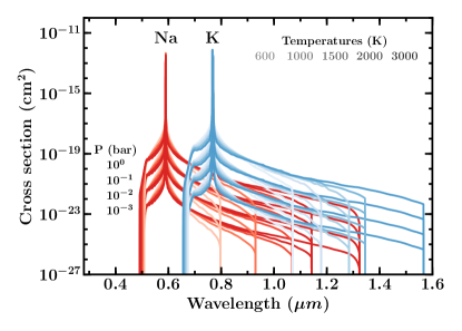
Figure 1: Absorption cross-sections of Na and K broadened by H₂ at different pressures and temperatures. Line profiles for each pressure appear as a group. In each group, the darker colors (broader wings) denote hotter temperatures.

4 Atmospheric Retrieval

We follow the retrieval approach in Welbanks & Madhusudhan (2019) based on the AURA retrieval code (Pinhas et al., 2018). The code allows for the retrieval of chemical abundances, a pressure-temperature profile, and cloud/haze properties using spectra from multiple instruments. The model computes line by line radiative transfer in a transmission geometry and assumes hydrostatic equilibrium and uniform chemical volume mixing ratios in the atmosphere. A full description of the retrieval setup can be found in Pinhas et al. (2019) and Welbanks & Madhusudhan (2019).

Besides the new H₂ broadened alkali species discussed in section 3, we include opacities due to other chemical species possible in hot giant planet atmospheres (Madhusudhan, 2012). Our retrievals generally consider absorption due to H₂O (Rothman et al., 2010), Na (Allard et al., 2019), K (Allard et al., 2016), CH₄ (Yurchenko & Tennyson, 2014), NH₃ (Yurchenko et al., 2011), HCN (Barber et al., 2014), CO (Rothman et al., 2010), and H₂-H₂ and H₂-He collision induced absorption (CIA; Richard et al., 2012). Additionally, following previous studies (Chen et al., 2018; von Essen et al., 2019; Sedaghati et al., 2017; MacDonald & Madhusudhan, 2019), we include absorption due to Li (Kramida et al., 2018) for WASP-127b, AlO (Patrascu et al., 2015) for WASP-33b, TiO (Schwenke, 1998) for WASP-19b, and CrH (Bauschlicher et al., 2001), TiO, and AlO for HAT-P-26b. We exclude absorption due to Na and K for K2-18b, GJ-3470b, and WASP-107b as it is not expected for these species to remain in gas phase at the low temperatures of these planets (e.g., Burrows & Sharp, 1999). The absorption cross-sections are calculated using the methods of Gandhi & Madhusudhan (2018).

The parameter estimation and Bayesian inference is conducted using the Nested Sampling algorithm implemented using PyMultiNest (Buchner et al., 2014). We choose log uniform priors for the volume mixing ratios of all species between -12 and -1. We further expand this prior to $-0.3$ for planets less massive than Saturn ($\sim 0.3$ M${}_{\text{J}}$) to allow for extremely high ($\sim$50%) H₂O abundances. The temperature prior at the top of the atmosphere is uniform with a lower limit at 0K for $\text{T}_{eq.}<900\text{K}$, $400\text{K}$ for $900\text{K}<\text{T}_{eq.}<1200\text{K}$ and $800\text{K}$ for $\text{T}_{eq.}>1200\text{K}$, and a higher limit at $\text{T}_{eq.}+100\text{K}$. Our retrieval of WASP-19b allows for a wavelength shift relative to the model for VLT FORS2 data only, as performed by Sedaghati et al. (2017). The retrievals performed in this study have in general 18 free parameters: 7 chemical abundances, 6 for the pressure-temperature profile, 4 for clouds and hazes, and 1 for the reference pressure at the measured observed radius of the planet.

Table 1: Planetary Properties and Retrieved H₂O, Na, and K Abundances (Mixing Ratio) for 19 Exoplanets

$\#$	Planet Name	M${}_{\text{p}}$(M${}_{\text{J}}$)	T${}_{\text{eq}}$ (K)	log(X${}_{\text{H}_{2}\text{O}}$)	DS${}_{\text{H}_{2}\text{O}}$	log(X${}_{\text{Na}}$)	DS${}_{\text{Na}}$	log(X${}_{\text{K}}$)	DS${}_{\text{K}}$
1	K2-18b	0.03	290	$-2.36^{+1.17}_{-1.16}$	3.26	N/A	N/A	N/A	N/A
2	GJ3470b	0.04	693	$-2.83^{+0.87}_{-0.77}$	3.75	N/A	N/A	N/A	N/A
3	HAT-P-26b	0.06	994	$-1.83^{+0.46}_{-0.57}$	8.61	$-9.08^{+2.04}_{-1.88}$	N/A	$-10.56^{+1.21}_{-0.96}$	N/A
4	HAT-P-11b	0.07	831	$-3.66^{+0.83}_{-0.57}$	4.12	$-9.36^{+2.04}_{-1.67}$	N/A	$-9.80^{+1.62}_{-1.42}$	N/A
5	WASP-107b	0.12	740	$-2.87^{+0.95}_{-0.73}$	5.70	N/A	N/A	N/A	N/A
6	WASP-127b	0.18	1400	$-2.13^{+0.65}_{-3.63}$	2.07	$-2.19^{+0.81}_{-4.41}$	3.66	$-2.89^{+0.80}_{-3.44}$	4.77
7	HAT-P-12b	0.21	960	$-5.70^{+1.22}_{-3.36}$	1.57	$-8.97^{+2.33}_{-1.94}$	N/A	$-8.33^{+2.32}_{-2.09}$	N/A
8	WASP-39b	0.28	1120	$-0.65^{+0.14}_{-1.83}$	8.92	$-3.62^{+1.14}_{-2.69}$	3.83	$-5.62^{+2.30}_{-2.05}$	2.37
8	WASP-39b∗	0.28	1120	$-2.43^{+0.27}_{-0.24}$	9.20	$-6.17^{+0.50}_{-0.51}$	3.97	$-7.24^{+0.71}_{-1.06}$	2.45
9	WASP-31b	0.48	1580	$-4.55^{+1.77}_{-4.33}$	1.65	$-8.08^{+2.28}_{-2.37}$	N/A	$-3.48^{+1.38}_{-2.31}$	2.89
10	WASP-96b	0.48	1285	$-4.95^{+2.25}_{-4.19}$	1.61	$-5.26^{+0.75}_{-0.59}$	5.16	$-9.27^{+1.46}_{-1.60}$	N/A
11	WASP-6b	0.50	1150	$-8.12^{+2.52}_{-2.41}$	N/A	$-8.25^{+3.10}_{-2.30}$	N/A	$-3.22^{+1.21}_{-3.79}$	2.55
12	WASP-17b	0.51	1740	$-3.84^{+1.27}_{-0.51}$	3.36	$-8.65^{+1.76}_{-1.67}$	1.09	$-9.62^{+1.78}_{-1.45}$	N/A
13	HAT-P-1b	0.53	1320	$-2.54^{+0.75}_{-0.67}$	3.17	$-8.58^{+1.20}_{-1.79}$	1.32	$-8.93^{+2.01}_{-1.93}$	N/A
14	HD 209458b	0.69	1450	$-4.54^{+0.33}_{-0.27}$	6.80	$-5.47^{+0.61}_{-0.48}$	6.77	$-7.00^{+0.59}_{-0.49}$	3.90
15	HD 189733b	1.14	1200	$-4.66^{+0.35}_{-0.33}$	5.26	$-4.19^{+0.67}_{-0.73}$	5.51	$-5.54^{+0.49}_{-0.44}$	3.34
16	WASP-19b	1.14	2050	$-3.43^{+0.47}_{-0.52}$	7.12	$-5.11^{+1.00}_{-1.05}$	3.48	$-10.85^{+1.20}_{-0.80}$	N/A
17	WASP-12b	1.40	2510	$-3.23^{+1.42}_{-0.80}$	5.41	$-6.64^{+2.13}_{-2.98}$	1.58	$-8.94^{+2.35}_{-1.92}$	N/A
18	WASP-43b	2.03	1440	$-3.68^{+0.92}_{-0.88}$	3.31	$-6.95^{+3.21}_{-3.22}$	N/A	$-7.50^{+3.02}_{-2.87}$	N/A
19	WASP-33b	2.10	2700	$-6.64^{+3.15}_{-3.25}$	1.29	$-8.98^{+2.28}_{-1.89}$	N/A	$-6.77^{+2.83}_{-3.16}$	N/A

Note. — The detection significance (DS) is included for each individual species. N/A means that the model without the chemical species had more evidence than the model including it (e.g., $B<1$), that the corresponding species was not included in the model or, in the case of WASP-43b, that it is not possible to provide a DS since no optical data was utilized. Planet mass and equilibrium temperature, with uniform redistribution, are quoted as nominal values; uncertainties in these values are not considered. WASP-39b^∗ corresponds to the case with an upper end of prior on the volume mixing ratios at -1 rather than -0.3.

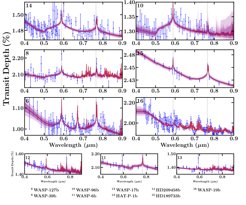
Figure 2: Observations and retrieved model transmission spectra of exoplanets showing evidence of Na and/or K in the optical wavelengths. Dotted lines show the wavelength positions for Na ($\sim 0.589\mu$m) and K ($\sim 0.770\mu$m). Observations are shown in blue while median retrieved models and confidence intervals (1$\sigma$ and 2$\sigma$) are shown in red and purple respectively. The top six panels show planets with evidence for Na or K above 2$\sigma$, and the bottom three show those with weaker evidence (see Table 1). Full optical and infrared spectra are available online at osf.io/nm84s.

5 Results

The atmospheric constraints for our sample of 19 transiting exoplanets, ranging from hot Jupiters to cool mini-Neptunes are shown in Table 1. The detection significance is calculated from the Bayes factor (Benneke & Seager, 2013; Buchner et al., 2014). We consider reliable abundance estimates to be those with detection significances larger than 2$\sigma$.

5.1 Abundances of H₂O, Na, and K

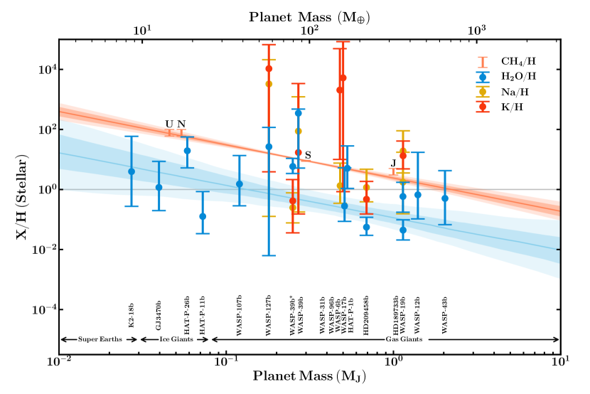
Figure 3: Mass-metallicity relation for planets with chemical detections above 2$\sigma$ significance (see Table 1). The H₂O/H, Na/H, and K/H abundances are shown in blue, yellow, and orange, respectively. All the abundances are normalized to expectations based on their host stars, as described in Section 5.1. The metallicity estimates for the solar system giant planets using their methane (CH₄) abundances (Atreya et al., 2016) are shown in coral. The coral shaded regions show the 1$\sigma$ and 2$\sigma$ metallicity trend for the solar system planets resulting from a linear fit. The corresponding fit to the exoplanet H₂O abundances, excluding WASP-39b (see Section 5.2), and the confidence intervals are shown in the blue line and sky blue shaded regions. The fits are $\log(\text{CH}_{4}\text{/H})=-1.11^{+0.11}_{-0.10}\log(\text{M/M}_{\text{J}})+0.38^{+0.06}_{-0.06}$ and $\log(\text{H}_{2}\text{O/H})=-1.09^{+0.34}_{-0.33}\log(\text{M/M}_{\text{J}})-0.95^{+0.21}_{-0.19}$. The alkali (H₂O) abundances for the sample are generally above (below) the solar system trend. Results for WASP-39b^∗ (see Table 1) and some labels have been offset in mass for clarity.

We confirm detections of H₂O, Na, and K in 14, 6, and 6 planets, respectively, at over 2$\sigma$ confidence, as shown in Table 1. Figure 2 shows the observed spectra and model fits for planets where at least one of either Na or K is detected. Our retrieved abundances (volume mixing ratios) for these species are broadly consistent with previous surveys and studies on each planet, as discussed in Sections 1 and 2. The abundances can be assessed relative to expectations from thermochemical equilibrium for solar elemental composition (Asplund et al., 2009). For solar composition (C/O = 0.54), at $\text{T}\gtrsim 1200$ K roughly half the oxygen is expected to be in H₂O, at 1 bar pressure (Madhusudhan, 2012). Thus, $\log(\text{X}_{\text{H}_{2}\text{O}})\sim-3.3$ and $-3.0$ for T above and below 1200 K, respectively. Similarly, $\log(\text{X}_{\text{Na}})=-5.76$, and $\log(\text{X}_{\text{K}})=-6.97$ for $\text{T}\gtrsim 1100\text{-}1200$ K, below which they enter molecular states (Burrows & Sharp, 1999). Figure 3 shows the abundances of Na, K, and H₂O relative to expectations based on their stellar elemental abundances as described above for solar composition. The stellar abundances (e.g. Brewer et al., 2016) used here are available at osf.io/nm84s. For stars without [Na/H], [O/H], or [K/H] estimates we adopt the [Fe/H] values.

The best constraints are obtained for H₂O across the sample, with precisions between $\sim 0.3$ and 1 dex for many of the planets, as shown in figure 3. The median H₂O abundances for most of the gas giants are substellar, with some being consistent to stellar values within $\sim 1\sigma$. On the other hand, smaller planets show an increase in H₂O abundances, albeit with generally larger uncertainties. In the ice giants and mini-Neptunes the median abundances are nearly stellar, with the exception of HAT-P-26b and HAT-P-11b, which are significantly superstellar and substellar, respectively. An exception is the hot Saturn WASP-39b for which anomalously high H₂O was reported with the latest data (Wakeford et al., 2018; Kirk et al., 2019). We find its abundance estimates to be sensitive to the choice of priors; we report two estimates with different priors in Table 1.

Contrary to H₂O, the median abundances of Na and K are nearly stellar or superstellar across the seven gas giants. The alkali abundances are retrieved only for the gas giants in our sample, with uncertainties larger than those for H₂O. For planets where they are nearly stellar (e.g., HD 209458b) Na and K are still more enhanced relative to H₂O, as with the other planets. The retrieved alkali abundances represent the population of ground state species. While previous studies noted the effect of non-LTE ionization on the absorption strength of alkali lines (Barman et al., 2002; Fortney et al., 2003), others (e.g., Fisher & Heng, 2019) show that the effect is less pertinent for interpretation of low-resolution spectra as in the present study. Our retrieved Na abundances are consistent with Fisher & Heng (2019) for the same planets. Nonetheless, as discussed in Welbanks & Madhusudhan (2019), the simplified model assumptions in Fisher & Heng (2019, e.g., isotherms, limited absorbers, and no CIA opacity) likely affect the precision and accuracy of their abundance constraints, perhaps explaining their unphysically high temperatures even in LTE. Furthermore, alkali broadening in Fisher & Heng (2019) is inconsistent with the more accurate broadening (Allard et al., 2019) used in the present work.

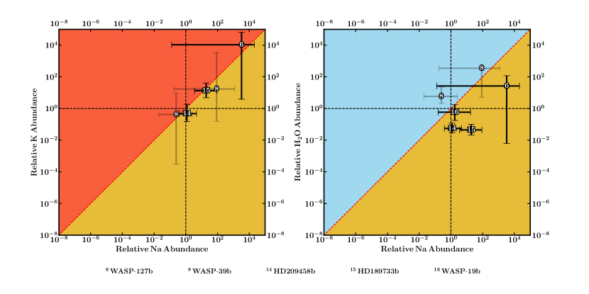
Figure 4: Normalized abundances of Na, K, and H₂O for detections above 2$\sigma$ significance. Left: K vs. Na abundances normalized by host stellar abundances. Right: normalized H₂O vs. Na abundances. Abundances are normalized following the description in Section 5.1. The red dashed diagonal line in each plot shows the ‘unity line’ where the normalized abundance ratio between species is equal to 1. The black dashed lines show individual normalized mixing ratios equal to 1. Two values are shown for WASP-39b corresponding to Table 1 in a lighter shade.

5.2 Abundance Ratios and Mass-Metallicity Relation

The abundances of Na, K, and H₂O provide constraints on their differential enhancements in hot gas giant atmospheres relative to their host stars. Figure 4 shows abundances of different species, relative to their host stars, compared against each other. Planets with significant indications of Na and K, i.e., WASP-127b, WASP-39b, HD 189733b, and HD 209458b, have a normalized K/Na ratio consistent with unity. Thus, the abundances of Na and K closely follow their stellar proportions; they are enhanced or depleted together in the planetary atmosphere relative to the star. On the contrary, the H₂O/Na ratios deviate significantly from their stellar expectations, especially for those planets with the tightest constraints: HD 209458b and HD 189733b. The right panel in figure 4 shows that for the small sample of planets with strong detections ($\gtrsim$2$\sigma$) of both Na and H₂O, most have preferential enhancement of Na relative to H₂O compared to stellar expectations; the only exception being WASP-39b. A similar trend can be inferred for H₂O/K, i.e., of K-enhancement and H₂O-depletion, given the Na/K ratios consistent with unity (left panel in figure 4). Given the present small sample of objects (N = 4) with strong detections of all three species (Na, K, and H₂O), future observations for more objects are required to further assess the Na/K trends seen here.

The H₂O abundances retrieved across our diverse sample of planets allow us to investigate a mass-metallicity relation for their atmospheres. In the solar system giant planets, CH₄ is thought to contain most of the carbon given their low temperatures. Thus, the CH₄ abundance has been used as a proxy for the carbon abundance and hence the metallicity (Atreya et al., 2016). A linear fit to the solar system CH₄ abundances leads to a ‘mass-metallicity’ relation of $\log(\text{CH}_{4}\text{/H})=-1.11^{+0.11}_{-0.10}\log(\text{M/M}_{\text{J}})+0.38^{+0.06}_{-0.06}$. As discussed in Section 5.1, the H₂O abundances in our exoplanet sample also show a gradually increasing trend with decreasing mass as shown in Fig. 3. However, the H₂O abundances across the entire sample, down to the mini-Neptunes, largely fall below the solar system metallicity trend based on CH₄ abundances. A linear fit to the exoplanetary H₂O abundances, excluding WASP-39b due to its strong prior dependence, yields an H₂O ‘mass-metallicity’ relation of $\log(\text{H}_{2}\text{O/H})=-1.09^{+0.34}_{-0.33}\log(\text{M/M}_{\text{J}})-0.95^{+0.21}_{-0.19}$, which is inconsistent with the solar system CH₄ measurements at over 6$\sigma$. On the other hand, the Na and K abundances for the gas giants are mostly consistent with the solar system carbon trend, albeit aided by their larger uncertainties.

6 Discussion

Our study reveals three key trends in the atmospheric compositions of our exoplanet sample. Firstly, from mini-Neptunes to hot Jupiters, H₂O abundances are generally consistent with or depleted compared to equilibrium expectations based on stellar abundances, and lower than the solar system metallicity trend. Second, the gas giants exhibit Na and K abundances consistent with or higher than those of their host stars and the solar system trend. Lastly, the Na and K elemental ratios are consistent with each other.

The overall low H₂O abundances across the sample contrasts with solar system predictions. Besides the carbon enhancements seen in the solar system (Fig. 3), other elements such as nitrogen, sulfur, phosphorous, and noble-gases are also enhanced in Jupiter (Atreya et al., 2016); the oxygen abundance is unknown as H₂O condenses at the low temperatures of solar system giants. Considering that oxygen is the most cosmically abundant element after H and He, it is expected to be even more enhanced than carbon in giant planets, according to solar system predictions (Mousis et al., 2012). Therefore, the consistent depletion of H₂O abundances in our sample suggest different formation pathways for these close-in exoplanets compared to the long-period solar system giants.

The H₂O abundance is likely representative of the oxygen abundance (O/H) for our cool Neptunes/mini-Neptunes. The H₂O abundance is less sensitive to C/O for T$\lesssim$1200 K, with most of the O bound in H₂O regardless of C/O (Madhusudhan, 2012). Thus, the H₂O abundances for our exo-Neptunes and mini-Neptunes (T$\lesssim$1200 K) indicate somewhat lower metallicities in their atmospheres than solar system expectations (Atreya et al., 2016). On the other hand, for hot gas giant photospheres (T$\gtrsim$1200 K), the H₂O abundance depends on both the O/H and C/O ratios. A C/O $\sim$ 1 can lead to $\sim$100$\times$ depletion in H₂O compared to solar C/O (0.54). Thus, even for a solar or super-solar O/H the H₂O in hot gas giants can be subsolar if the C/O is high.

The low H₂O abundances in hot gas giants are therefore unlikely to be due to low O/H or low overall metallicities, considering the higher alkali enrichments in some planets. An atmosphere depleted up to 100$\times$ in O/H while being enriched in other elements is unlikely (Madhusudhan et al., 2014a). Instead, the H₂O underabundance and alkali enrichment are likely due to superstellar C/O, Na/O, and K/O ratios, i.e., an overall stellar or superstellar metallicity but oxygen depleted relative to other species. This addresses the degeneracy between C/O and metallicity prevalent since the first inferences of low H₂O abundances in hot Jupiters (Madhusudhan et al., 2014b).

These H₂O abundances in hot gas giants, while generally inconsistent with expectations from solar system and similar predictions for exoplanets (e.g. Mousis et al., 2012; Thorngren et al., 2016), could suggest other formation pathways. The combination of stellar or superstellar metallicities and high C/O ratios in hot Jupiters can instead be caused by primarily accreting high C/O gas outside the H₂O and CO₂ snow lines (Öberg et al., 2011; Madhusudhan et al., 2014a). The high Na and K abundances could potentially be caused by accretion of planetesimals rich in alkalis at a later epoch, potentially even in close-in orbits. Another possibility is the formation of giant planets by accreting metal-rich and high C/O gas caused by pebble drift (Öberg & Bergin, 2016; Booth et al., 2017). Future studies could further investigate these avenues to explain the observed trends.

Finally, our study highlights important lessons for the interpretation of atmospheric spectra of gas giants. The differing trends in the abundances of species argue against the use of chemical equilibrium models with the metallicity and C/O ratio as the only free chemical parameters in atmospheric retrievals; different elements can be differently enhanced. Atmospheric models also need to consider the effect of H₂ broadening of alkali opacities on abundance estimates. With better quality data and targeted observations, comparative atmospheric characterization of exoplanets as pursued here will likely continue to unveil trends that may inform us about their formation and evolutionary mechanisms.

7 Acknowledgements

LW thanks the Gates Cambridge Trust for support towards his doctoral studies. NM acknowledges support from the Science and Technology Facilities Council (STFC) UK. We thank Dr. Kaisey Mandel for helpful discussions. We thank the anonymous reviewer for their thoughtful comments on the manuscript. This research is made open access thanks to the Bill & Melinda Gates foundation.

Here we present a subset of the supplementary material included online. Further information, tables, and figures are included in osf.io/nm84s.

Appendix A Supplementary information

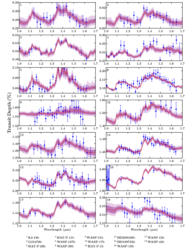
Figure A.1: Observations and retrieved model transmission spectra of exoplanets showing evidence of H₂O in the near infrared wavelengths. Observations are shown in blue while median retrieved models and confidence intervals (1$\sigma$ and 2$\sigma$) are shown in red and purple respectively. Planets are ordered by increasing mass. All planets shown, except WASP-31b, have a H₂O absorption feature with an evidence above 2$\sigma$ (see Table 1). These observations were obtained with the HST WFC3 spectrograph. Full optical and infrared spectra are available online at osf.io/nm84s.

References

- Allard et al. (1999) Allard, N. F., Royer, A., Kielkopf, J. F., & Feautrier, N. 1999, Phys. Rev. A, 60, 1021
- Allard et al. (2016) Allard, N. F., Spiegelman, F., & Kielkopf, J. F. 2016, A&A, 589, A21
- Allard et al. (2019) Allard, N. F., Spiegelman, F., Leininger, T., & Molliere, P. 2019, A&A, 628, A120
- Asplund et al. (2009) Asplund, M., Grevesse, N., Sauval, A. J., & Scott, P. 2009, ARA&A, 47, 481
- Atreya et al. (2016) Atreya, S. K., Crida, A., Guillot, T., et al. 2016, arXiv e-prints, arXiv:1606.04510
- Barber et al. (2014) Barber, R. J., Strange, J. K., Hill, C., et al. 2014, MNRAS, 437, 1828
- Barman et al. (2002) Barman, T. S., Hauschildt, P. H., Schweitzer, A., et al. 2002, ApJ, 569, L51
- Barstow et al. (2017) Barstow, J. K., Aigrain, S., Irwin, P. G. J., & Sing, D. K. 2017, ApJ, 834, 50
- Bauschlicher et al. (2001) Bauschlicher, C. W., Ram, R. S., Bernath, P. F., Parsons, C. G., & Galehouse, D. 2001, The Journal of Chemical Physics, 115, 1312. https://doi.org/10.1063/1.1377892
- Benneke & Seager (2013) Benneke, B., & Seager, S. 2013, ApJ, 778, 153
- Benneke et al. (2019a) Benneke, B., Knutson, H. A., Lothringer, J., et al. 2019a, Nature Astronomy, 3, 813
- Benneke et al. (2019b) Benneke, B., Wong, I., Piaulet, C., et al. 2019b, arXiv e-prints, arXiv:1909.04642
- Booth et al. (2017) Booth, R. A., Clarke, C. J., Madhusudhan, N., & Ilee, J. D. 2017, MNRAS, 469, 3994
- Brewer et al. (2016) Brewer, J. M., Fischer, D. A., Valenti, J. A., & Piskunov, N. 2016, ApJS, 225, 32
- Buchner et al. (2014) Buchner, J., Georgakakis, A., Nandra, K., et al. 2014, A&A, 564, A125
- Burrows & Sharp (1999) Burrows, A., & Sharp, C. M. 1999, ApJ, 512, 843
- Chachan et al. (2019) Chachan, Y., Knutson, H. A., Gao, P., et al. 2019, AJ, 158, 244
- Charbonneau et al. (2002) Charbonneau, D., Brown, T. M., Noyes, R. W., & Gilliland, R. L. 2002, ApJ, 568, 377
- Chen et al. (2017) Chen, G., Guenther, E. W., Pallé, E., et al. 2017, A&A, 600, A138
- Chen et al. (2018) Chen, G., Pallé, E., Welbanks, L., et al. 2018, A&A, 616, A145
- Espinoza et al. (2019) Espinoza, N., Rackham, B. V., Jordán, A., et al. 2019, MNRAS, 482, 2065
- Fisher & Heng (2019) Fisher, C., & Heng, K. 2019, ApJ, 881, 25
- Fortney et al. (2003) Fortney, J. J., Sudarsky, D., Hubeny, I., et al. 2003, ApJ, 589, 615
- Fu et al. (2017) Fu, G., Deming, D., Knutson, H., et al. 2017, ApJ, 847, L22
- Gandhi & Madhusudhan (2018) Gandhi, S., & Madhusudhan, N. 2018, MNRAS, 474, 271
- Heng (2016) Heng, K. 2016, ApJ, 826, L16
- Kirk et al. (2019) Kirk, J., López-Morales, M., Wheatley, P. J., et al. 2019, AJ, 158, 144
- Kramida et al. (2018) Kramida, A., Yu. Ralchenko, Reader, J., & and NIST ASD Team. 2018, NIST Atomic Spectra Database (ver. 5.6.1), [Online]. Available: https://physics.nist.gov/asd [2019, February 6]. National Institute of Standards and Technology, Gaithersburg, MD., ,
- Kreidberg et al. (2014) Kreidberg, L., Bean, J. L., Désert, J.-M., et al. 2014, ApJ, 793, L27
- MacDonald & Madhusudhan (2019) MacDonald, R. J., & Madhusudhan, N. 2019, MNRAS, 486, 1292
- Madhusudhan (2012) Madhusudhan, N. 2012, ApJ, 758, 36
- Madhusudhan et al. (2014a) Madhusudhan, N., Amin, M. A., & Kennedy, G. M. 2014a, ApJ, 794, L12
- Madhusudhan et al. (2014b) Madhusudhan, N., Crouzet, N., McCullough, P. R., Deming, D., & Hedges, C. 2014b, ApJ, 791, L9
- Mordasini et al. (2016) Mordasini, C., van Boekel, R., Mollière, P., Henning, T., & Benneke, B. 2016, ApJ, 832, 41
- Mousis et al. (2012) Mousis, O., Lunine, J. I., Madhusudhan, N., & Johnson, T. V. 2012, ApJ, 751, L7
- Nikolov et al. (2018) Nikolov, N., Sing, D. K., Fortney, J. J., et al. 2018, Nature, 557, 526
- Öberg & Bergin (2016) Öberg, K. I., & Bergin, E. A. 2016, ApJ, 831, L19
- Öberg et al. (2011) Öberg, K. I., Murray-Clay, R., & Bergin, E. A. 2011, ApJ, 743, L16
- Patrascu et al. (2015) Patrascu, A. T., Yurchenko, S. N., & Tennyson, J. 2015, MNRAS, 449, 3613
- Pinhas et al. (2019) Pinhas, A., Madhusudhan, N., Gandhi, S., & MacDonald, R. 2019, MNRAS, 482, 1485
- Pinhas et al. (2018) Pinhas, A., Rackham, B. V., Madhusudhan, N., & Apai, D. 2018, MNRAS, 480, 5314
- Redfield et al. (2008) Redfield, S., Endl, M., Cochran, W. D., & Koesterke, L. 2008, ApJ, 673, L87
- Richard et al. (2012) Richard, C., Gordon, I. E., Rothman, L. S., et al. 2012, J. Quant. Spec. Radiat. Transf., 113, 1276
- Rothman et al. (2010) Rothman, L. S., Gordon, I. E., Barber, R. J., et al. 2010, J. Quant. Spec. Radiat. Transf., 111, 2139
- Schwenke (1998) Schwenke, D. W. 1998, Faraday Discussions, 109, 321
- Sedaghati et al. (2017) Sedaghati, E., Boffin, H. M. J., MacDonald, R. J., et al. 2017, Nature, 549, 238
- Sing et al. (2016) Sing, D. K., Fortney, J. J., Nikolov, N., et al. 2016, Nature, 529, 59
- Spake et al. (2018) Spake, J. J., Sing, D. K., Evans, T. M., et al. 2018, Nature, 557, 68
- Stevenson (2016) Stevenson, K. B. 2016, ApJ, 817, L16
- Stevenson et al. (2016) Stevenson, K. B., Bean, J. L., Seifahrt, A., et al. 2016, ApJ, 817, 141
- Stevenson et al. (2017) Stevenson, K. B., Line, M. R., Bean, J. L., et al. 2017, AJ, 153, 68
- Thorngren et al. (2016) Thorngren, D. P., Fortney, J. J., Murray-Clay, R. A., & Lopez, E. D. 2016, ApJ, 831, 64
- von Essen et al. (2019) von Essen, C., Mallonn, M., Welbanks, L., et al. 2019, A&A, 622, A71
- Wakeford et al. (2017) Wakeford, H. R., Sing, D. K., Kataria, T., et al. 2017, Science, 356, 628
- Wakeford et al. (2018) Wakeford, H. R., Sing, D. K., Deming, D., et al. 2018, AJ, 155, 29
- Welbanks & Madhusudhan (2019) Welbanks, L., & Madhusudhan, N. 2019, AJ, 157, 206
- Wyttenbach et al. (2015) Wyttenbach, A., Ehrenreich, D., Lovis, C., Udry, S., & Pepe, F. 2015, A&A, 577, A62
- Yurchenko et al. (2011) Yurchenko, S. N., Barber, R. J., & Tennyson, J. 2011, MNRAS, 413, 1828
- Yurchenko & Tennyson (2014) Yurchenko, S. N., & Tennyson, J. 2014, MNRAS, 440, 1649