Asymptotic based bootstrap approach for matched pairs with missingness in a single-arm

Abstract

The issue of missing values is an arising difficulty when dealing with paired data. Several test procedures are developed in the literature to tackle this problem. Some of them are even robust under deviations and control type-I error quite accurately. However, most these methods are not applicable when missing values are present only in a single arm. For this case, we provide asymptotic correct resampling tests that are robust under heteroscedasticity and skewed distributions. The tests are based on a clever restructuring of all observed information in a quadratic form-type test statistic. An extensive simulation study is conducted exemplifying the tests for finite sample sizes under different missingness mechanisms. In addition, an illustrative data example based on a breast cancer gene study is analyzed.

1 Introduction

Conducting statistical tests on units measured repeatedly requires the consideration of the dependence structure of the resulting random vector. The simplest design is the matched pairs model, where units are measured at two endpoints of the same subject. This design has experienced a large field of application, including industrial and life sciences. In Biomedicine for example, several studies have been focused on identifying genes for up- or down regulated effects in head and neck squamous, prostate, lung or breast cell carcinoma.kuriakose2004selection ; lapointe2004gene ; feng2008dna In common statistical analysis, testing the equality of means in matched pairs design is conducted using the paired t-test. Even for non-normal data, the procedure is asymptotically exact, i.e. for sufficiently large samples, the test procedure is correctly reflecting type-I-error. However, first limitation of the paired t-test arises when data is only partially observed. Deleting observations with missing values is a sub-optimal solution, since variance or mean estimation based only on complete case analysis can be biased leading to incorrect statistical inference. This is especially the case when complete samples are small.

To tackle this issue, a simple approach is to impute missing values singly (or multiply) and to carry out statistical tests as if there were no missing values so farschafer1999multiple ; rubin2004multiple ; sterne2009multiple . However, although leading to good imputation error stekhoven2011missforest ; waljee2013comparison ; Ramosaj2019 , such approaches may lead to inflated type-I error rate or remarkably low power in small to moderate sample sizes ramosaj2018caution ; van2018flexible . Therefore, we do not follow this approach here.

Differing to imputation, several test procedures that (only) use all observed information in the matched pairs design have been proposed in the literature mehta1969testing ; lin1973procedures ; morrison1973test ; lin1974difference ; little1976inference ; ekbohm1976comparing ; bhoj1978testing ; looney2003method ; kim2005statistical ; samawi2014notes ; uddin2017testing . These tests, however, rely on specific model assumptions such as symmetry or even bivariate normality, which are hard to verify in practice. Moreover, these procedures are usually non robust to deviations and may results in inaccurate decisions caused by possibly conservative or inflated type-I error rates samawi2014notes ; amro2017permuting ; amro2019multiplication ; qi2018testing .

To overcome these problems, the typical recommendation is to use the method based on combining separate results of adequate test statistics for the underlying paired and unpaired portions of the data using either weighted test statisticssamawi2014notes ; amro2017permuting , a multiplication combination test amro2019multiplication , or combined p-values rempala2006asymptotic ; samawi2011nonparametric ; yu2012permutation ; kuan2013simple . However, all these methods are only applicable for matched pairs with missingness in both arms. Thus, these methods cannot be used to analyze data on pathological stage I breast cancer patients from the Cancer Genome Atlas (TCGA) project. This data set consists of observations from $90$ patients of which $74$ had entries in one component of it, only $16$ were complete, see Section 7 below for details. The question is now how to analyze such data?.

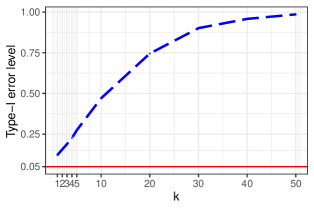
Figure 1: Type-I error simulation results ($\alpha=0.05$) of the nonparametric combination test $T_{NC}$ $({\color[rgb]{0,0,1}\textendash\textendash\quad\textendash\textendash})$ for exponential distribution under correlation factor ($\rho=0.7$) and a heteroscedastic set-up with variances $1$ and $2$ respectively for increasing sample sizes $k\cdot(n_{c},n_{u})=(k\cdot 10,k\cdot 30)$ under the MCAR framework.

In contrast to the above methods, barely any work can be found that is potentially applicable in this special missing pattern, requires no parametric assumptions and also leads to valid inferences in case of heteroscedasticity or skewed distributions. One exception is given by the recent proposals of Qi et. al. qi2018testing who recommended a so-called nonparametric combination test (NCT). It is based on merging results from Sign test and Wilcoxon Mann-Whitney test. In situations where these two nonparametric procedures show their efficiency, their proposed combination is indeed tempting. However, neither the Sign test is known to be very powerful for metric data nor is the Mann-Whitney test known for being robust against heteroscedasticity. In fact, our simulation studies demonstrate that their NCT inherits these unsatisfying properties to some extend. It show that, under heteroscedasticity and/or skewed distributions, the test statistic (NCT) tends not to maintain the pre-assigned type-I error level. The degree of variance heterogeneity, skewness, and sample sizes can all affect the type-I error rate control level. An overview of the type-I error control of NCT when heteroscedasticity coincides with a skewed error distribution is displayed in Figure  1. It reveals that, under heteroscedasticity and exponential distribution, the NCT type-I error rate function becomes surprisingly analogous to the power function where the type-I error rate increases dramatically with an increase in sample sizes.

The aim of this paper is therefore bilateral: First, we aim to provide a statistical test that is capable of treating single arm missing values in matched pairs which drops the common assumptions such as homoscedasticity and normality and secondly, is able to satisfactorily control type-I-error while maintaining good power properties. To this end, we propose three different test statistics, analyze their asymptotic behaviors under the null hypothesis and equip them with an asymptotically correct parametric bootstrap procedure for calculating critical values. In doing so, we structured the paper by firstly introducing the statistical model and the hypothesis of interest. In Section 3, we provide different test statistics of quadratic form-type that either converge to a $\chi^{2}$ or a weighted $\chi^{2}$ distributions. Proofs presenting theoretical guarantees of the proposed methods are delivered in the supplement. In Section 4, we introduce a parametric bootstrap technique to calculate critical values and prove it’s theoretical correctness. Section 5 is devoted to already existing methods for statistical inference in matched pairs with single arm missingness while in Section 6 and 7, novel and existing methods are compared based on an extensive simulation study and a real data example from a breast cancer gene study. The supplement contains additional analyses.

2 Statistical Model and Hypotheses

We consider matched pairs given by a sample $\mathcal{D}_{n}:=\{\mathbf{X}_{1},\dots,\mathbf{X}_{n}\}$, where $\mathbf{X}_{j}=(X_{1j},X_{2j})^{T}\in\mbox{$\mathbb{R}$}^{2}$ are i.i.d. random vectors with mean vector $\mathbb{E}[\mathbf{X}_{1}]=\boldsymbol{\mu}=[\mu_{1},\mu_{2}]^{\top}\in\mbox{$\mathbb{R}$}^{2}$ and an arbitrary covariance matrix $0<\boldsymbol{\Gamma}\in\mbox{$\mathbb{R}$}^{2\times 2}$. To incorporate missingness in one arm (says, the second) only denote with $R_{2j}\in\{0,1\}$, $j=1,\dots,n$ the vector whose $j$-th component indicates whether $X_{2j}$ is observed $(R_{2j}=1)$ or missing $(R_{2j}=0)$ for $j=1,\dots,n$. If $*$ denotes the component-wise multiplication of vectors, then in practice, one observes $\mathbf{X}^{(o)}:=\{\mathbf{X}_{j}*\mathbf{R}_{j}\}_{j=1}^{n}$ where $\mathbf{R}_{j}=[1,R_{2j}]^{\top}\in\mbox{$\mathbb{R}$}^{2}$ , $j=1,\dots,n$, and a ”$0$” entry is interpreted as missing. Hence our framework has the following form, where $---$ stands as a placeholder for $R_{2j}=0$:

$$\begin{gathered}\underbrace{\begin{bmatrix}[c]X_{11}^{(c)}\\ X_{21}^{(c)}\end{bmatrix},\dots,\begin{bmatrix}[c]X_{1n_{c}}^{(c)}\\ X_{2n_{c}}^{(c)}\end{bmatrix}}_{\mathbf{X}^{(c)}},\underbrace{\begin{bmatrix}[c]X_{11}^{(i)}\\ \text{ }_{---}\end{bmatrix},\dots,\begin{bmatrix}[c]X_{1n_{u}}^{(i)}\\ \text{ }_{---}\end{bmatrix}}_{\mathbf{X}^{(i)}}\end{gathered}$$ (1)

Rubin defines the missing mechanism through a parametric distributional model on $\mathbf{R}=\{\mathbf{R}_{j}\}_{j=1}^{n}$ and classifies their presence through Missing Completely at Random (MCAR), Missing at Random (MAR) and Missing not at Random (MNAR) schemes.rubin2004multiple In our work, we first assume a MCAR mechanism, in that $\boldsymbol{X}^{c}$ is independent of $\boldsymbol{X}^{(i)}$. However, we will also study MAR mechanisms in simulations and relate to the supplement for the explicit definition of the missing mechanisms. For notational purposes, let $I_{n_{c}}$ denote the index set of $\lvert I_{n_{c}}\rvert=n_{c}$ complete pairs, i.e. $\mathbf{R}_{j}=[1,1]^{\top}$ for all $j\in I_{n_{c}}$. Similarly, $I_{n_{u}}$ is the index set of observations with second component missing $(\mathbf{R}_{j}=[1,0]^{\top},j\in I_{n_{u}})$ and $\lvert I_{n_{u}}\rvert=n_{u}$. Thus, there are in total $N=2n_{c}+n_{u}$ observations from $n=n_{c}+n_{u}$ subjects.
In this framework, we like to use all the available data to test the null hypothesis $H_{0}:$ $\{\mu_{1}=\mu_{2}\}$ of equal means against the alternative $H_{1}:$ {$\mu_{1}\neq\mu_{2}$}.

To construct our paper test statistics, we first fix estimators of the population means $\mu_{1}$, and $\mu_{2}$. For estimating $\mu_{1}$, we consider two estimators; the sample mean of the first components of the completed data set $\bar{X}_{1.}^{(c)}=\frac{1}{n_{c}}\sum_{i=1}^{n_{c}}X_{1i}^{(c)}$, and the sample mean of the first components of the unpaired data $\bar{X}_{1.}^{(i)}=\frac{1}{n_{u}}\sum_{j=1}^{n_{u}}X_{1j}^{(i)}$. For estimating the population mean $\mu_{2}$, we use the sample mean of the second components of the complete data $\bar{X}_{2.}^{(c)}=\frac{1}{n_{c}}\sum_{i=1}^{n_{c}}X_{2i}^{(c)}$.

Next, we define the normalized vector $\boldsymbol{Z}_{n}$ that aggregates the difference between the mean values $\boldsymbol{\mu}=[\mu_{1},\mu_{2}]^{\top}$ and their empirical estimators $[\bar{X}_{1.}^{(c)},\bar{X}_{2.}^{(c)},\bar{X}_{1.}^{(i)}]^{\top}$

$$\boldsymbol{Z}_{n}=\sqrt{n}[\bar{X}_{1.}^{(c)}-\mu_{1},\bar{X}_{2.}^{(c)}-\mu_{2},\bar{X}_{1.}^{(i)}-\mu_{1}]^{\top}$$ (2)

and take their correlations into account in the covariance matrix $\boldsymbol{\Sigma}_{n}=Cov(\boldsymbol{Z}_{n})$.

For subsequently asymptotic analyses, we need to set up the following assumption regarding sample sizes, which we assume throughout

Assumption 1.

For $\min\{n_{c},n_{u}\}\to\infty$ we require that

• $\frac{n_{c}}{n_{c}+n_{u}}\to\kappa_{1}\in(0,1)$

• $\frac{n_{u}}{n_{c}+n_{u}}\to\kappa_{2}=(1-\kappa_{1})\in(0,1)$

Proposition 2.1.

Let $\sigma_{1}^{2}=Var(X_{11}^{(c)})=Var(X_{11}^{(i)})$, $\sigma_{2}^{2}=Var(X_{21}^{(c)})$ and $\rho=corr(X_{11}^{(c)},X_{21}^{(c)})$. The statistic $\boldsymbol{Z}_{n}$ has, asymptotically, as $n\to\infty$, a multivariate normal distribution with expectation $0$ and covariance matrix given by

$$\boldsymbol{\Sigma}=\lim_{n\to\infty}\boldsymbol{\Sigma}_{n}=\begin{bmatrix}\kappa_{1}^{-1}\sigma_{1}^{2}&\kappa_{1}^{-1}\rho\sigma_{1}\sigma_{2}&0\\ \kappa_{1}^{-1}\rho\sigma_{1}\sigma_{2}&\kappa_{1}^{-1}\sigma^{2}_{2}&0\\ 0&0&\kappa_{2}^{-1}\sigma^{2}_{1}\end{bmatrix}.$$ (3)

$\boldsymbol{\Sigma}_{n}$ can be consistently estimated by

$$\hat{\boldsymbol{\Sigma}}_{n}=\begin{bmatrix}\hat{\kappa}_{1}^{-1}\hat{\sigma}^{2}_{1}&\hat{\kappa}_{1}^{-1}\hat{\rho}\hat{\sigma}_{1}\hat{\sigma}_{2}&0\\ \hat{\kappa}_{1}^{-1}\hat{\rho}\hat{\sigma}_{1}\hat{\sigma}_{2}&\hat{\kappa}_{1}^{-1}\hat{\sigma}^{2}_{2}&0\\ 0&0&\hat{\kappa}_{2}^{-1}\hat{\sigma}^{2}_{1}\end{bmatrix},$$ (4)

where $\hat{\kappa}_{1}=n_{c}/n$, $\hat{\kappa}_{2}=n_{u}/n$ and $\hat{\sigma}_{1}^{2}$ is the unbiased empirical variance estimator based on the pooled first components $X_{11}^{(c)},\dots,X_{1n_{c}}^{(c)},X_{11}^{(i)},\dots,X_{1n_{u}}^{(i)}$, $\hat{\sigma}_{2}^{2}=\frac{1}{n_{c}-1}\sum\limits_{i=1}^{n_{c}}(X_{2i}^{(c)}-\bar{X}_{2\cdot}^{(c)})^{2}$ and the correlation factor $\rho$ is estimated through the empirical correlation $\hat{\rho}$ calculated from the paired data $\mathbf{X}^{(c)}$.

To test the null hypothesis $H_{0}:\mu_{1}-\mu_{2}=0$, we define the two estimators $\bar{X}_{1.}^{(c)}-\bar{X}_{2.}^{(c)}$ and $\bar{X}_{1.}^{(i)}-\bar{X}_{2.}^{(c)}$ for $\mu_{1}-\mu_{2}$. Their joined asymptotic behavior under the null hypothesis $H_{0}$ is studied below.

Proposition 2.2.

Set $f_{\boldsymbol{A}}(\mathbf{x})=\boldsymbol{A}\mathbf{x}$, for the matrix ${\boldsymbol{A}}=\begin{bmatrix}1&-1&0\\ 0&-1&1\end{bmatrix}$ $\in\mbox{$\mathbb{R}$}^{2X3}$. Then, under the null hypothesis $H_{0}$, the composite statistic

$$f_{\boldsymbol{A}}\circ\boldsymbol{Z}_{n}=\mathbf{A}\mathbf{Z}_{n}=\sqrt{n}[\bar{X}_{1.}^{(c)}-\bar{X}_{2.}^{(c)},\bar{X}_{1.}^{(i)}-\bar{X}_{2.}^{(c)}]^{\top},$$ (5)

is asymptotically $N_{2}(\mathbf{0},\mathbf{A}\boldsymbol{\Sigma}\mathbf{A}^{\top})$ distributed as $n\rightarrow\infty$.

3 Statistics and Asymptotics

In this section, we propose three different quadratic forms for testing $H_{0}$: a Wald-type statistic (WTS), an ANOVA-type statistic (ATS), and a modified ANOVA-type statistic (MATS). To introduce the WTS, denote by $\mathbf{B}^{+}$ the Moore-Penrose inverse of a matrix $\mathbf{B}$. Then, the WTS is given by

$$T_{W}=(\boldsymbol{A}\boldsymbol{Z}_{n})^{\top}(\boldsymbol{A}\hat{\boldsymbol{\Sigma}}_{n}\boldsymbol{A}^{\top})^{+}(\boldsymbol{A}\boldsymbol{Z}_{n}).$$ (6)

Thanks to the introduced studentization by $(\boldsymbol{A}\hat{\boldsymbol{\Sigma}}_{n}\boldsymbol{A}^{\top})^{+}$, the WTS is asymptotically distribution-free as studied below.

Theorem 3.1.

The statistic $T_{W}$ has under the null hypothesis $H_{0}:\{\mu_{1}=\mu_{2}\}$, asymptotically, as $n\to\infty$, a central $\chi^{2}_{2}$ distribution.

Similar WTS versions are also studied in the context of heteroscedastic ANOVA or MANOVA krishnamoorthy2010parametric ; xu2013parametric ; konietschke2015parametric ; friedrich2018mats . From these settings, it is known that the convergence to its limiting $\chi^{2}$-distribution is rather slow vallejo2010analysis ; konietschke2015parametric ; smaga2017bootstrap , which leads to several refinements regarding bootstrapping for the calculations of critical values (see Section 4 below) or other structures of test statistics. In particular, Brunner (2001) brunner2001asymptotic proposed an alternative quadratic form by deleting the Moore-Penrose inverse involved in the computation of the WTS, resulting in the following ATS:

$$T_{A}=\frac{1}{tr(\mathbf{A}\hat{\boldsymbol{\Sigma}}_{n}\mathbf{A}^{\top})}(\mathbf{A}\boldsymbol{Z}_{n})^{\top}(\mathbf{A}\boldsymbol{Z}_{n}),$$ (7)

which is also applicable in case of $|\hat{\boldsymbol{\Sigma}}_{n}|=0$.

Theorem 3.2.

Under the null hypothesis $H_{0}:\{\mu_{1}=\mu_{2}\}$, the test statistic $T_{A}$ has asymptotically, as $n\to\infty$, the same distribution as the random variable

$$Y=\sum_{i=1}^{2}\lambda_{i}Y_{i}/tr(\mathbf{A}\boldsymbol{\Sigma}\mathbf{A}^{\top}),$$ (8)

where $Y_{i}\overset{\text{i.i.d}}{\sim}\chi^{2}_{1}$ and the weights $\lambda_{i}$ are the eigenvalues of $\boldsymbol{A}\boldsymbol{\Sigma}\mathbf{A}^{\top}$ where $\boldsymbol{\Sigma}$ is given in (3).

Another possible test statistic would be the modified version of the ANOVA type-statistic (MATS) that was developed by Friedrich and Pauly (2017) friedrich2018mats for MANOVA models. Here, it is given by

$$T_{M}=(\boldsymbol{A}\boldsymbol{Z}_{n})^{\top}\hat{\boldsymbol{D}}_{n}(\boldsymbol{A}\boldsymbol{Z}_{n}),$$ (9)

where $\hat{\boldsymbol{D}}_{n}=diag((\mathbf{A}\hat{\boldsymbol{\Sigma}}_{n}\mathbf{A}^{\top})^{+}_{ii})$.

Theorem 3.3.

Under the null hypothesis $H_{0}:\{\mu_{1}=\mu_{2}\}$, the test statistic $T_{M}$ has asymptotically,as $n\to\infty$, the same distribution as the random variable

$$\tilde{Y}=\sum_{i=1}^{2}\tilde{\lambda}_{i}\tilde{Y}_{i},$$ (10)

where $\tilde{Y}_{i}\overset{\text{i.i.d}}{\sim}\chi_{1}^{2}$ and the weights $\tilde{\lambda}_{i}$ are the eigenvalues of $\mathbf{D}\mathbf{A}\boldsymbol{\Sigma}\mathbf{A}^{\top}$ and $\mathbf{D}=diag((\mathbf{A}\boldsymbol{\Sigma}\mathbf{A}^{\top})^{+}_{ii})$.

As, the weights $\lambda_{i}$, and $\tilde{\lambda}_{i}$ in Theorems 3.2 and 3.3 are unknown and the $\chi_{2}^{2}-$approximation to $T_{W}$ is rather slow, we will develop adequate and asymptotically correct testing procedures based on bootstrap versions of $T_{W},T_{A},$ and $T_{M}$ in the subsequent section.

4 Parametric Bootstrapping

To estimate critical values, we apply an asymptotic model based bootstrap approach which has , e.g. been applied in the context of (M)ANOVA factorial designs friedrich2018mats ; konietschke2015parametric . To this end, first, we generate parametric bootstrap variables as

$$\mathbf{X}^{*}_{j}=\begin{bmatrix}X_{1j}^{*}\\ X_{2j}^{*}\end{bmatrix}\overset{\text{i.i.d}}{\sim}N(0,\hat{\boldsymbol{\Gamma}}),j=1,...,n.$$ (11)

Here, $\hat{\boldsymbol{\Gamma}}=\begin{bmatrix}\hat{\sigma}_{1}^{2}&\hat{\rho}\hat{\sigma}_{1}\hat{\sigma}_{2}\\ \hat{\rho}\hat{\sigma}_{1}\hat{\sigma}_{2}&\hat{\sigma}_{2}^{2}\end{bmatrix}$ is an empirical covariance matrix estimator, where $\hat{\sigma}_{1}^{2}$, $\hat{\sigma}_{2}^{2}$ and $\hat{\rho}$ are as in Proposition 2.1. The idea is to reflect the original covariance structure to obtain more accurate finite sample approximation. Next, we generate missing values under the MCAR scheme by randomly inserting them to the second component of the bivariate vector $\mathbf{X}^{*}_{j}$ until a fixed amount of missing values of size $n_{u}$ is achieved. This results into the following bootstrapped data set

$$\begin{gathered}\underbrace{\begin{bmatrix}X_{11}^{*(c)}\\ X_{21}^{*(c)}\end{bmatrix},\dots,\begin{bmatrix}X_{1n_{c}}^{*(c)}\\ X_{2n_{c}}^{*(c)}\end{bmatrix}}_{\mathbf{X}^{*(c)}},\underbrace{\begin{bmatrix}X_{11}^{*(i)}\\ \text{ }_{---}\end{bmatrix},\dots,\begin{bmatrix}X_{1n_{u}}^{*(i)}\\ \text{ }_{---}\end{bmatrix}}_{\mathbf{X}^{*(i)}}\end{gathered}$$ (12)

and the combined vector $(f\circ\boldsymbol{Z}_{n})^{*}=\boldsymbol{A}\boldsymbol{Z}_{n}^{*}=\sqrt{n}(\bar{X}_{1.}^{*(c)}-\bar{X}_{2.}^{*(c)},\bar{X}_{1.}^{*(i)}-\bar{X}_{2.}^{*(c)})$. From this, the bootstrapped versions of the quadratic forms, i.e. the Wald-type statistic $T_{W}^{*}$, the ANOVA-type statistic $T_{A}^{*}$ and the modified ANOVA-type statistic $T_{M}^{*}$ are computed

$$T_{W}^{*} =(\boldsymbol{A}\boldsymbol{Z}_{n}^{*})^{\top}(\mathbf{A}\hat{\boldsymbol{\Sigma}}^{*}_{n}\mathbf{A}^{T})^{+}(\boldsymbol{A}\boldsymbol{Z}_{n}^{*}),$$ (13)

$$T_{A}^{*} =\frac{1}{tr(\mathbf{A}\hat{\boldsymbol{\Sigma}}^{*}_{n}\mathbf{A}^{\top})}(\boldsymbol{A}\boldsymbol{Z}_{n}^{*})^{\top}(\boldsymbol{A}\boldsymbol{Z}_{n}^{*}),$$ (14)

$$T_{M}^{*} =(\boldsymbol{A}\boldsymbol{Z}_{n}^{*})^{\top}\hat{\boldsymbol{D}}^{*}_{n}(\boldsymbol{A}\boldsymbol{Z}_{n}^{*}),$$ (15)

where $\hat{\boldsymbol{\Sigma}}^{*}_{n}=\hat{\boldsymbol{\Sigma}}_{n}(\mathbf{X}^{*(c)},\mathbf{X}^{*(i)})$ and $\hat{\boldsymbol{D}}^{*}_{n}=diag((\mathbf{A}\hat{\boldsymbol{\Sigma}}_{n}^{*}\mathbf{A}^{\top})^{+}_{ii})$.

The next theorem proves that all three bootstrapped test statistics can be used to approximate the null distribution of the respective test statistic.

Theorem 4.1.

For any choice $[-]\in\{A,M,W\}$, the conditional distribution of $T_{[-]}^{*}$ converges weakly to the null distribution of $T_{[-]}$ in probability for any choice of $\boldsymbol{\mu}\in\mbox{$\mathbb{R}$}^{2}$ and $\boldsymbol{\mu}_{0}\in H_{0}$. In particular we have

$$\sup_{x\in\mbox{$\mathbb{R}$}}|P_{\boldsymbol{\mu}}(T_{[-]}^{*}\leq x|\boldsymbol{X})-P_{\boldsymbol{\mu}_{0}}(T_{[-]}\leq x)|\xrightarrow{\text{p}}0.$$

From Theorem 4.1, we thus obtain the asymptotically correct bootstrap tests $\varphi_{W}^{*}=\mathds{1}\{T_{W}>c_{W}^{*}\},\varphi_{A}^{*}=\mathds{1}\{T_{A}>c_{A}^{*}\}$, and $\varphi_{M}^{*}=\mathds{1}\{T_{M}>c_{M}^{*}\}$ where $c_{W}^{*},c_{A}^{*},$ and $c_{M}^{*}$ denote the conditional $(1-\alpha)$- bootstrap quantiles of $T_{W}^{*},T_{A}^{*}$, and $T_{M}^{*}$ respectively.

To analyze their finite sample performance, we below conduct extensive simulations (Section 6). Before that, we will first discuss other possible candidates from the literature that should or should not be included in our simulation study.

5 Comparison with existing methods

We briefly review the existing literature on methods that can deal with the case of matched pairs with missing values in one arm only. As outlined in the introduction, there only exists a few which we can summarize them as follows

1. Simple methods such as: using the paired t-test while excluding the unpaired data OR using the independent t-test while ignoring the covariance structure of the data.

2. Tests based on modified maximum likelihood estimators. morrison1973test ; ekbohm1976oncomparing ; little1976inference

3. Tests based on simple mean difference estimator. lin1973procedures ; mehta1969testing ; mehta1973test ; ekbohm1976oncomparing

4. P-values pooling methods.qi2018testing

5. Weighted linear and nonlinear combination tests.qi2018testing

However, none of the methods is free from distributional assumptions and at the same time robust against deviations such as heteroscedasticity and skewed distributions. In particular, the recent paper by Qi et al.qi2018testing already included a simulation study to compare several of the tests mentioned in (a) - (e). As a conclusion, they recommended a so-called non-parametric combination test (NCT).

Therefore, we will mainly focus on the non-parametric combination method proposed in Qi et al.qi2018testing As additional competitor for these bootstrap procedures proposed in Section 4, we choose the test of Little. little1976inference The latter assumes that the data follows a bivariate normal distribution and the test statistic is given by

$$T_{LT} =\frac{\bar{X}_{1\cdot}-\bar{X}_{2\cdot}^{(c)}-\frac{\hat{\rho}\hat{\sigma}_{1}^{(c)}\hat{\sigma}_{2}}{(\hat{\sigma}_{1}^{(c)})^{2}}(\bar{X}_{1\cdot}-\bar{X}_{1\cdot}^{(c)})}{\hat{\sigma}_{\mathbf{LT}}},$$ (16)

where $\bar{X}_{1}:=1/n(n_{c}\bar{X}_{1\cdot}^{(c)}+n_{u}\bar{X}_{1\cdot}^{(i)})$ and $\hat{\sigma}_{1}^{(c)}$ is the empirical standard deviation of $\{X_{11}^{(c)},\dots,X_{1n_{c}}^{(c)}\}$. Moreover, setting $\hat{\sigma}_{22\cdot 1}^{2}=\hat{\sigma}_{2}^{2}-(\hat{\rho}\hat{\sigma}_{1}^{(c)}\hat{\sigma}_{2}/(\hat{\sigma}_{1}^{(c)})^{2})$ and $\hat{\sigma}_{\mathbf{X}}=\hat{\sigma}_{22\cdot 1}^{2}+\frac{(\hat{\rho}\hat{\sigma}_{1}^{(c)}\hat{\sigma}_{2})^{2}}{(\hat{\sigma}_{1}^{(c)})^{4}}\hat{\sigma}_{1}^{4}$, the denominator is given by little1976inference

$$\hat{\sigma}_{\mathbf{LT}}^{2} =\frac{\hat{\sigma}_{\mathbf{X}}^{2}}{n}+\left(\frac{1}{n_{c}}-\frac{1}{n}\right)\frac{n_{c}-2}{n_{c}-3}\hat{\sigma}_{22\cdot 1}^{2}-\frac{2}{n}\frac{\hat{\rho}\hat{\sigma}_{1}^{(c)}\hat{\sigma}_{2}}{(\hat{\sigma}_{1}^{(c)})^{2}}\hat{\sigma}_{1}^{2}+\frac{\hat{\sigma}_{1}^{2}}{n}$$

The exact distribution of $T_{LT}$ is rather complicated and Little suggests to approximate it by a $t$-reference distribution with $n_{c}-1$ degrees of freedom, i.e. the test is given by $\varphi_{LT}:=\mathds{1}\{|T_{LT}|>t_{n_{c}-1,1-\alpha/2}\}$ for some level $\alpha\in(0,1)$.

In addition, the non-parametric combination testqi2018testing proposed by Qi et al., is based upon a linear combination of the sign and the Wilcoxon Mann-Whitney test statistics:

$$T_{NC}=T_{s}+T_{m},$$ (17)

where $T_{s}=\frac{1}{n_{c}}\sum_{i=1}^{n_{c}}\phi(X_{1i}^{(c)},X_{2i}^{(c)})$ and $T_{m}=\frac{1}{n_{c}n_{u}}\sum_{j=1}^{n_{u}}\sum_{k=1}^{n_{c}}\phi(X_{1j}^{(i)},X_{2k}^{(c)})$ with

$\phi(X_{1},X_{2})=\begin{cases}1&\text{if}\;X>Y\\ 1/2&\text{if}\;X=Y\\ 0&\text{otherwise.}\end{cases}$

It is proposed qi2018testing to approximate the null distribution of $T_{NC}$ by a normal distribution with mean $1$ and variance estimated by $\widehat{Var}(T_{NC})=\frac{1}{n_{c}}+\frac{n_{c}+n_{u}+1}{12n_{c}n_{u}}+\widehat{Cov}(T_{s},T_{m})$, where
$\widehat{Cov}(T_{s},T_{m})=\frac{1}{n_{c}^{2}n_{u}}\sum_{i=1}^{n_{c}}\sum_{j=1}^{n_{u}}\mathds{1}\{X_{1i}^{(c)}>X_{2i}^{(c)},X_{1j}^{(i)}>X_{2j}^{(c)}\}-\frac{1}{n_{c}}T_{s}T_{m}$.

Table 1: Type-I error simulation results ($\alpha=0.05$) of the tests for different distributions under varying correlation values ($\rho$) with sample sizes $(n_{c},n_{u})\in\{(10,10),(30,10),(10,30)\}$ and homoscedastic covariance matrix $\Sigma_{1}$ under the MCAR framework. For each setting, the values closest to the prescribed level are printed in bold and values exceeding the upper limit ($6.8\%$) of the $99\%$ binomial interval are in red colour.

Dist	$\rho$	$(10,10)$						$(30,10)$						$(10,30)$
		$T_{W}^{*}$	$T_{A}^{*}$	$T_{M}^{*}$	$T_{NC}$	$T_{LT}$		$T_{W}^{*}$	$T_{A}^{*}$	$T_{M}^{*}$	$T_{NC}$	$T_{LT}$		$T_{W}^{*}$	$T_{A}^{*}$	$T_{M}^{*}$	$T_{NC}$	$T_{LT}$
Normal	-0.9	5.4	5.5	5.4	6.8	4.4		5.2	5.2	5.2	5.6	5.5		5.5	5.4	6.7	6.8	4.0
	-0.5	5.1	5.4	5.7	6.5	4.9		5.0	5.2	5.1	5.5	5.3		5.5	5.6	6.4	6.7	5.1
	-0.1	5.4	5.6	5.4	6.6	5.6		5.6	5.3	5.4	5.4	5.6		5.3	5.6	6.1	6.8	6.0
	0.1	5.2	5.5	5.5	6.4	6.1		5.0	4.5	4.5	4.9	5.3		5.2	5.5	5.8	6.5	6.1
	0.5	5.1	5.0	4.8	6.0	6.8		4.9	5.2	4.9	5.6	5.6		5.0	5.1	4.9	6.2	6.5
	0.9	5.3	5.3	4.6	5.8	12.3		4.8	5.0	4.6	4.8	12.0		5.4	5.4	4.3	6.1	8.0
Laplace	-0.9	4.6	4.9	5.4	6.6	4.6		4.4	4.8	4.5	5.2	4.9		4.6	4.7	6.0	6.8	3.1
	-0.5	4.3	4.8	5.0	6.5	4.6		4.4	4.7	5.0	5.1	5.1		4.3	5.0	5.8	6.7	4.3
	-0.1	4.3	5.0	4.8	6.5	5.4		4.0	4.7	4.7	5.2	5.4		4.6	4.9	5.3	6.4	5.3
	0.1	4.4	4.7	4.6	6.6	5.2		4.5	4.9	5.0	5.4	5.4		4.3	4.8	5.3	6.4	5.6
	0.5	4.3	4.5	4.4	6.2	6.4		4.3	4.3	4.5	5.2	5.2		4.3	4.5	4.9	6.6	5.7
	0.9	4.2	5.2	4.0	6.1	13.3		4.5	4.7	4.2	5.0	14.3		4.3	5.1	4.0	6.1	9.4
Exp	-0.9	4.5	4.2	5.2	6.4	4.2		5.3	5.0	6.0	5.7	5.4		4.6	4.2	6.1	6.7	3.9
	-0.5	5.2	4.9	5.0	6.6	5.0		6.9	4.7	6.4	5.2	5.0		5.0	4.7	6.4	6.2	5.4
	-0.1	4.8	4.4	4.2	6.1	5.8		7.0	4.7	6.2	5.2	5.1		7.3	5.9	7.5	7.0	7.8
	0.1	5.4	4.9	4.5	6.4	7.2		6.8	4.9	6.4	5.4	5.7		7.5	5.7	7.1	6.4	8.1
	0.5	5.7	4.3	4.2	6.5	9.4		5.8	5.0	5.6	5.4	6.4		8.4	6.0	6.8	6.1	10.8
	0.9	6.4	4.8	3.8	6.1	15.3		5.0	5.1	4.6	4.9	15.6		10.0	6.6	4.9	6.4	16.2
Chisq	-0.9	5.2	5.4	5.5	6.4	4.3		5.3	5.0	5.2	5.5	5.2		5.0	5.4	6.6	6.6	3.7
	-0.5	4.6	5.1	5.2	6.3	4.7		5.1	4.9	5.0	5.2	4.7		4.9	5.2	6.0	6.4	4.6
	-0.1	5.4	5.6	5.5	6.7	5.9		5.1	4.6	5.0	5.3	5.2		5.5	5.7	6.2	6.6	5.6
	0.1	5.2	5.2	5.0	6.3	5.5		5.2	4.8	5.0	5.0	5.4		5.8	5.8	6.0	6.4	6.5
	0.5	4.9	4.8	4.7	6.2	6.3		5.0	4.7	4.8	5.1	5.6		5.7	5.0	5.3	6.0	6.8
	0.9	5.6	5.3	4.5	5.7	12.8		5.4	5.6	5.2	5.4	12.6		5.8	5.3	4.5	6.0	8.9

Table 2: Type-I error simulation results ($\alpha=0.05$) of the tests for different distributions under varying correlation values ($\rho$) with sample sizes $(n_{c},n_{u})\in\{(10,10),(30,10),(10,30)\}$ and heteroscedastic covariance matrix $\Sigma_{2}$ under the MCAR framework. For each setting, the values closest to the prescribed level are printed in bold and values exceeding the upper limit ($6.8\%$) of the $99\%$ binomial interval are in red colour.

Dist	$\rho$	$(10,10)$						$(30,10)$						$(10,30)$
		$T_{W}^{*}$	$T_{A}^{*}$	$T_{M}^{*}$	$T_{NC}$	$T_{LT}$		$T_{W}^{*}$	$T_{A}^{*}$	$T_{M}^{*}$	$T_{NC}$	$T_{LT}$		$T_{W}^{*}$	$T_{A}^{*}$	$T_{M}^{*}$	$T_{NC}$	$T_{LT}$
Normal	-0.9	5.5	5.5	5.7	7.0	4.7		4.8	5.1	5.0	4.6	5.2		5.5	5.4	7.0	7.8	4.1
	-0.5	5.1	5.6	5.8	7.2	5.1		5.2	5.2	5.2	5.0	5.3		5.5	5.6	6.7	7.4	5.6
	-0.1	5.5	5.8	5.7	7.1	6.0		4.8	4.9	4.8	4.4	5.1		5.4	5.7	6.4	7.8	6.4
	0.1	5.2	5.5	5.6	6.8	6.2		4.6	4.8	5.0	4.7	5.5		5.2	5.6	6.0	7.2	6.6
	0.5	5.4	5.2	5.2	6.4	7.0		5.2	5.0	5.0	4.9	5.4		5.0	5.6	5.8	7.4	6.7
	0.9	5.4	5.4	6.1	6.4	12.4		5.1	4.9	5.2	4.8	11.0		5.0	6.0	7.2	6.9	7.7
Laplace	-0.9	4.6	4.8	5.6	7.2	4.8		4.5	4.7	4.8	4.8	5.1		4.6	4.6	6.3	7.5	3.3
	-0.5	4.5	4.8	5.2	6.8	4.8		4.4	4.8	5.2	4.7	5.0		4.2	4.8	6.1	7.4	4.5
	-0.1	4.5	5.0	5.2	6.7	5.7		4.1	5.0	5.0	4.9	5.3		4.5	4.8	5.5	7.0	5.6
	0.1	4.6	4.8	4.9	7.0	5.4		4.4	4.9	5.2	4.7	5.4		4.3	5.1	5.8	7.2	5.8
	0.5	4.2	4.6	4.6	6.7	6.4		4.2	4.6	4.5	4.7	5.0		4.0	4.7	5.8	7.2	6.0
	0.9	4.1	5.3	5.3	6.8	13.9		4.4	4.7	4.8	4.5	14.8		4.0	5.2	6.6	6.9	8.7
Exp	-0.9	4.6	5.2	6.2	9.1	5.2		5.3	5.5	6.4	9.1	5.7		5.1	5.1	7.3	9.5	5.0
	-0.5	5.3	6.0	6.2	9.4	6.0		6.6	4.9	6.3	9.2	5.5		6.3	6.4	8.2	9.7	7.5
	-0.1	5.4	6.2	5.6	9.9	7.3		6.5	4.6	6.0	10.8	5.8		8.0	7.9	9.3	11.1	9.8
	0.1	6.4	7.0	6.1	10.0	8.9		6.2	4.6	6.0	11.4	6.2		8.3	7.9	8.7	10.9	9.8
	0.5	6.9	6.4	6.5	10.5	11.0		6.3	4.7	6.1	12.2	7.2		9.3	8.4	9.0	11.2	12.1
	0.9	8.1	5.8	8.8	12.2	18.2		6.9	4.5	7.0	17.6	17.6		10.2	8.2	11.5	13.6	15.8
Chisq	-0.9	5.2	5.4	5.8	7.1	4.4		5.4	5.2	5.0	4.9	5.3		5.3	5.4	7.0	7.6	3.8
	-0.5	4.6	5.3	5.3	6.9	5.0		5.2	4.7	4.8	5.0	5.1		4.9	5.5	6.6	7.4	5.2
	-0.1	5.5	6.0	5.9	7.2	6.6		5.1	4.9	5.0	4.9	5.4		5.6	5.8	6.5	7.7	6.2
	0.1	5.0	5.4	5.1	6.6	5.9		5.2	5.0	4.9	4.8	5.6		5.8	5.9	6.5	7.3	7.0
	0.5	5.0	5.5	5.4	6.9	6.8		5.1	4.9	5.0	5.1	5.6		5.8	5.5	6.0	7.2	7.2
	0.9	5.8	5.3	6.3	7.1	13.0		5.5	5.2	5.7	5.0	11.9		5.5	5.5	7.4	7.4	8.3

6 Simulation Study

In this section, we investigate the finite sample behavior of the methods described in Sections 4 and 5 in extensive simulations. All procedures were studied with respect to their

1. type-I-error rate control at level $\alpha=5\%$ and their

2. power to detect deviations from the null hypothesis.

Small to moderate sized paired data samples were generated from the model

$\mathbf{X}_{j}=\boldsymbol{\Sigma}^{\frac{1}{2}}\boldsymbol{\epsilon}_{j}+\boldsymbol{\mu},\quad j=1,...,n,$

where $\boldsymbol{\epsilon}_{j}=[\epsilon_{1j},\epsilon_{2j}]^{\top}$ is an i.i.d. bivariate random vector with mutually independent components and $E(\boldsymbol{\epsilon_{1}})=0$ and $Cov(\boldsymbol{\epsilon_{1}})=I_{2}$.

Different choices of symmetric as well as skewed residuals are considered such as standardized normal, exponential, Laplace and the $\chi^{2}$ distribution with $df=30$ degrees of freedom. For the covariance matrix $\boldsymbol{\Sigma}$, we considered the choices

$\boldsymbol{\Sigma_{1}}=\begin{bmatrix}[c]1&\rho\\ \rho&1\end{bmatrix}\text{ and }\boldsymbol{\Sigma_{2}}=\begin{bmatrix}[c]1&\sqrt{2}\rho\\ \sqrt{2}\rho&2\end{bmatrix}\textbf{}.$

with varying correlation factor $\rho\in(-1,1)$, representing a homoscedastic and a heteroscedastic covariance setting, respectively. The sample sizes were chosen as $(n_{c},n_{u})\in\{(10,10),(30,10),(10,30)\}$ under a MCAR mechanism and $n\in\{10,20,30\}$ under a MAR mechanism.

For each scenario, we generated missings as described below: For the MCAR mechanism, missing values are inserted randomly to the second component of the bivariate vector $\mathbf{X}_{j}$ until a fixed amount of missing values of size $n_{u}$ for the second component is achieved.

Table 3: Type-I error simulation results ($\alpha=0.05$) of the tests for different distributions under varying correlation values ($\rho$), different total sample sizes $n\in\{10,20,30\}$ (numbers of subjects) and homoscedastic covariance matrix $\Sigma_{1}$ under the MAR framework. For each setting, the values closest to the prescribed level are printed in bold and values exceeding the upper limit ($6.8\%$) of the $99\%$ binomial interval are in red colour.

Dist	$\rho$	$n=10$						$n=20$						$n=30$
		$T_{W}^{*}$	$T_{A}^{*}$	$T_{M}^{*}$	$T_{NC}$	$T_{LT}$		$T_{W}^{*}$	$T_{A}^{*}$	$T_{M}^{*}$	$T_{NC}$	$T_{LT}$		$T_{W}^{*}$	$T_{A}^{*}$	$T_{M}^{*}$	$T_{NC}$	$T_{LT}$
Normal	-0.9	5.4	3.7	5.2	6.4	3.6		5.4	5.1	5.7	5.8	5.5		5.1	5.4	6.0	5.7	5.5
	-0.5	4.8	3.9	4.4	6.4	4.6		5.3	4.9	5.5	5.6	5.2		5.2	5.1	5.8	5.3	5.1
	-0.1	4.6	4.1	4.4	6.2	5.7		5.1	4.7	5.0	5.5	5.5		5.0	5.0	5.1	5.3	5.2
	0.1	4.7	4.3	4.3	6.7	6.2		4.9	4.3	5.0	5.1	5.9		5.2	4.4	5.3	5.3	5.5
	0.5	4.7	4.2	4.1	6.3	7.3		5.2	5.0	5.1	5.5	6.4		5.3	4.8	5.0	4.8	5.9
	0.9	4.9	4.9	4.3	6.5	12.5		5.0	4.8	4.6	5.3	14.2		5.1	5.1	4.8	5.0	12.6
Laplace	-0.9	4.2	3.2	5.1	6.1	3.2		4.3	4.9	6.0	5.3	5.0		4.9	5.1	6.5	5.3	5.0
	-0.5	3.1	3.6	3.5	6.2	3.9		4.2	4.6	5.5	5.5	5.0		4.4	5.0	6.0	5.3	5.0
	-0.1	3.1	3.2	3.1	6.3	4.8		3.9	3.9	4.6	5.1	4.7		4.4	4.3	4.9	5.0	5.0
	0.1	3.2	2.7	3.0	6.3	5.6		4.1	3.7	4.6	5.6	5.3		4.6	4.4	5.3	5.2	5.6
	0.5	3.5	3.1	3.0	6.3	7.8		4.5	4.0	4.2	5.2	5.6		4.5	3.6	4.2	4.8	5.3
	0.9	3.6	3.9	3.3	5.6	11		4.0	4.1	3.8	4.9	14.4		4.5	4.4	4.3	4.6	14.4
Exp	-0.9	4.3	2.8	5.6	6.1	3.2		5.6	5.0	7.8	5.0	5.3		6.0	5.1	8.7	5.5	5.3
	-0.5	4.8	3.0	4.2	6.6	4.1		7.6	4.9	7.4	5.7	5.4		8.9	5.3	8.7	5.2	5.3
	-0.1	4.3	2.7	3.4	6.5	5.2		7.4	4.2	6.4	5.4	5.2		8.8	5.4	8.0	5.6	5.4
	0.1	4.0	2.6	3.4	6.5	6.2		7.1	4.3	6.5	5.6	5.9		8.1	5.4	7.6	5.5	5.1
	0.5	3.5	2.7	3.2	6.5	10.1		5.7	4.8	5.7	5.7	6.9		6.5	6.1	6.5	5.6	5.6
	0.9	4.3	4.7	4.2	5.8	10.2		5.0	5.7	5.2	5.2	13.4		5.6	6.9	5.7	5.2	15.3
Chisq	-0.9	4.6	3.7	4.5	5.6	3.7		5.1	5.3	5.9	5.9	5.5		5.0	5.2	6.0	5.4	5.3
	-0.5	4.5	3.7	4.4	6.3	4.3		5.1	4.8	5.4	5.4	5.3		5.4	4.8	5.5	5.3	5.3
	-0.1	4.7	3.8	4.4	6.6	5.7		5.3	4.7	5.3	5.2	5.8		5.7	5.1	5.7	5.4	5.6
	0.1	4.8	3.7	4.1	6.1	6.1		5.1	4.1	4.7	5.3	5.5		5.3	4.8	5.3	5.0	5.2
	0.5	4.2	3.8	3.6	6.0	7.3		4.9	4.4	4.8	5.3	6.1		4.9	4.7	4.8	4.9	5.0
	0.9	4.5	4.6	3.8	5.5	12.8		4.9	5.3	4.5	4.9	14.7		5.2	5.2	4.9	5.2	13.0

Table 4: Type-I error simulation results ($\alpha=0.05$) of the tests for different distributions under varying correlation values ($\rho$), different total sample sizes $n\in\{10,20,30\}$ (numbers of subjects) and heteroscedastic covariance matrix $\Sigma_{2}$ under the MAR framework. For each setting, the values closest to the prescribed level are printed in bold and values exceeding the upper limit ($6.8\%$) of the $99\%$ binomial interval are in red colour.

Dist	$\rho$	$n=10$						$n=20$						$n=30$
		$T_{W}^{*}$	$T_{A}^{*}$	$T_{M}^{*}$	$T_{NC}$	$T_{LT}$		$T_{W}^{*}$	$T_{A}^{*}$	$T_{M}^{*}$	$T_{NC}$	$T_{LT}$		$T_{W}^{*}$	$T_{A}^{*}$	$T_{M}^{*}$	$T_{NC}$	$T_{LT}$
Normal	-0.9	5.1	4.1	4.9	6.3	4.0		5.2	5.4	5.9	5.1	5.5		5.4	5.6	6.5	5.2	5.6
	-0.5	5.1	4.4	5.2	6.8	5.2		5.1	5.3	5.9	5.3	5.4		4.6	5.2	5.8	4.8	5.2
	-0.1	4.9	4.4	4.5	6.3	6.0		5.1	5.2	5.5	5.2	5.6		5.1	5.0	5.4	4.5	5.3
	0.1	5.2	4.5	4.5	6.6	6.5		5.3	5.1	5.5	5.4	6.5		5.1	4.7	5.2	4.5	5.1
	0.5	4.4	4.0	4.0	6.3	7.3		5.1	4.9	5.2	5.2	6.0		5.2	4.8	5.2	5.0	5.9
	0.9	4.6	4.8	5.0	7.0	14.7		4.9	4.7	5.3	5.2	14.1		5.0	5.0	5.3	4.6	11.8
Laplace	-0.9	4.0	3.4	5.2	6.3	3.6		4.2	4.9	6.8	4.8	5.0		4.4	5.1	7.4	4.8	5.3
	-0.5	3.2	3.6	4.1	6.0	4.2		4.5	5.0	6.4	5.4	5.2		4.7	4.9	6.7	4.9	4.8
	-0.1	3.1	3.7	4.0	6.5	5.4		3.9	4.5	5.3	5.3	5.2		4.7	5.0	6.1	4.8	5.1
	0.1	3.1	2.8	3.0	5.9	5.7		4.2	4.3	5.1	5.0	5.5		4.3	5.0	5.9	4.9	5.8
	0.5	3.4	3.4	3.4	6.5	8.1		4.2	4.0	4.5	5.1	6.0		4.4	4.6	5.1	4.6	5.6
	0.9	3.3	4.1	3.9	6.6	13.1		4.3	4.9	5.1	5.2	16.2		4.7	4.9	5.5	4.9	15.3
Exp	-0.9	3.3	4.0	6.0	7.4	4.3		4.7	5.7	9.0	7.4	6.0		5.3	5.5	8.6	7.7	5.6
	-0.5	4.2	4.1	4.1	7.8	5.4		6.5	5.5	7.0	7.2	6.4		8.4	5.8	8.5	8.2	6.2
	-0.1	4.5	3.5	3.8	8.2	7.0		6.9	4.7	6.2	7.4	6.2		8.6	5.6	7.9	9.0	6.3
	0.1	3.9	3.5	3.5	8.6	8.5		6.3	4.4	6.1	7.7	6.7		7.8	5.2	7.2	8.8	5.9
	0.5	4.6	2.9	4.2	7.8	11.0		6.3	4.5	6.3	8.1	8.4		6.9	5.2	7.0	9.3	7.3
	0.9	7.8	4.0	7.8	8.7	15.9		7.7	4.5	8.1	8.6	17.5		8.1	5.4	7.7	10.4	17.2
Chisq	-0.9	5.1	4.2	5.3	6.1	4.3		5.8	5.8	6.6	5.8	5.9		5.2	5.5	6.6	5.0	5.6
	-0.5	4.8	4.5	5.1	6.2	5.1		5.1	4.7	5.5	5.1	5.2		5.3	5.1	6.0	5.0	5.0
	-0.1	4.5	4.3	4.7	6.5	6.3		5.3	5.2	5.7	5.2	5.6		6.1	5.5	6.1	5.4	5.8
	0.1	4.3	4.0	4.0	6.3	6.6		5.0	4.8	5.2	5.2	5.8		5.1	5.1	5.5	4.9	5.6
	0.5	4.7	3.9	4.3	6.5	7.6		5.4	4.8	5.3	5.6	6.5		5.5	4.8	5.5	5.1	5.8
	0.9	4.9	4.5	5.0	7.0	15		5.3	4.8	5.4	5.6	15.2		5.7	5.1	5.6	5.1	13.3

For the MAR mechanism, the probability of being missing on the the second component of $\mathbf{X}_{j}$ is based on the corresponding value on the first component in the following way: first, we divide $\mathbf{X}$ into three groups based on their first component values corresponding to a $2\sigma-$rule: the first group is given by $\{\boldsymbol{X}_{j}=(X_{1j},X_{2j}):X_{1j}\in(-\infty,-2\widehat{\sigma}_{1}),j=1,..,n\}$, the second by $\{\boldsymbol{X}_{j}:X_{1j}\in(-2\widehat{\sigma}_{1},2\widehat{\sigma}_{1}),j=1,..,n\}$ and the last group by $\{\boldsymbol{X}_{j}:X_{1j}\in(2\widehat{\sigma}_{1},\infty),j=1,..,n\}$, where $\widehat{\sigma}_{1}$ is the estimated sample variance from all first components. Then, we randomly insert missing values on the second component based on the following missing percentages: $15\%$ for group one and three and $30\%$ for the second group .

In order to assess the power of all methods, we set $\boldsymbol{\mu}=[\delta,0]^{\top}$ with shift parameter $\delta\in\{0,1/2,1\}$. All simulations were operated by means of the statistical computing environment R based on $n_{sim}=10,000$ Monte-Carlo runs and $B=1,000$ bootstrap runs (in case of the three bootstrapped methods based upon $T_{W}^{*},T_{A}^{*}$, and $T_{M}^{*}$). The algorithm for the computation of the $p$-value of the parametric bootstrap tests is as follows:

1. For the given incomplete paired data, calculate the observed test statistic, say $T$.

2. Estimate the covariance matrix $\boldsymbol{\Gamma}$ by $\hat{\boldsymbol{\Gamma}}$.

3. Generate a bootstrap sample $\mathbf{X}^{*}_{j}=(X_{1j}^{*},X_{2j}^{*})$ from $N(\boldsymbol{0},\hat{\boldsymbol{\Gamma}})$, $j=1,...,n$.

4. Insert missing values in a MCAR or MAR manner to the second component of the vector $\mathbf{X}^{*}_{j}$ resulting in $\mathbf{X}^{*(c)}_{j}$ and $\mathbf{X}^{*(i)}_{k}$ where $j=1,\dots,n_{c},$ $k=1,\dots,n_{u}$.

5. Calculate the value of the test statistic for the bootstrapped sample $T^{*}$.

6. Repeat the Steps $3$ and $4$ independently $B=1,000$ times and collect the observed test statistic values in ${T^{*}_{b},b=1,.....,B}$.

7. Finally, estimate the bootstrap $p$-value as $p-value=\frac{\sum_{b=1}^{B}I(T^{*}_{b}>=T)}{B}$.

Type-I-Error Results. Simulation results of type-I error level of the studied procedures under the MCAR framework for different sample sizes and for homoscedastic as well as heteroscedastic settings are summarized in Table 1 and Table 2 respectively.
It can be readily seen that the suggested bootstrap approaches based upon $T_{W}^{*},T_{A}^{*}$ and $T_{M}^{*}$ tend to result in quite accurate type-I error rate control under homoscedasticity as well as heteroscedasticity and over the whole range of correlation factors for most settings. Only in two cases; First, in case of the negative unbalanced sample size $(10,30)$, particularly under heteroscedasticity, the bootstrapped MATS ($T_{M}^{*}$) is not recommended due to it’s liberal behavior. However, in such case, the other two suggested bootstrapped tests $T_{W}^{*}$, and $T_{A}^{*}$ are controlling type-I error rate accurately. Secondly, in case of the skewed exponential distribution, the control is not adequate and a liberal behavior is observed. However, in this case, all the other chosen procedures also failed to control type-I error rate for the underlying sample sizes, which are indicated in bold red through all tables. Specifically, in the case of homoscedasticity, and a balanced sample size $(10,10)$, our three suggested tests still result in accurate test decisions. For a positive balanced sample size $(30,10)$, the bootstrapped ANOVA ($T_{A}^{*}$) still controls type-I error rate accurately under homoscedastic as well heteroscedastic settings. It has even the best control of type-I error rate among all considered methods that are identified by bold entries in the table.

In contrast, the other tests ($T_{NC}$, $T_{LT}$) do not control type-I error level constantly under heteroscedasticity or even under homoscedasticity in all of the considered sample sizes. It can also be seen from Table 1 and Table 2 that the nonparametric combination test $T_{NC}$, controls type-I error quite accurately in the case of larger numbers of complete pairs $(n_{c}=30)$, but it shows liberal behavior for smaller numbers of complete pairs $(n_{c}=10)$. This test turns very liberal in the case of heteroscedasticity. Moreover, the test that is based on the maximum likelihood estimator $T_{LT}$ tends to result in a very liberal decision in the case of smaller numbers of complete pairs together with positive correlation factors $\rho$. For larger numbers of complete pairs, it leads to an accurate type-I error rate control for correlation factors being less than $0.5$. This behavior of the test does not depend on the homoscedasticity assumption.

It was also interesting to discover the type-I error rate control of the tests under similar attributes to the breast cancer gene study data which reflects data sets with a few pairs and large amount of unpaired portions. Simulation results for the type-I error rate of the studied procedures for $(n_{c}=16,n_{u}=74)$ sample sizes are presented in Table S.3 and Table S.4 in the supplement. The correlation $\rho$ in Table S.4 is estimated based on the data It can be easily seen from Table S.3 and Table S.4 that the bootstrap tests are robust under large amounts of missing observations and control type-I error rate accurately, especially the bootstrapped tests $T_{W}^{*}$, and $T_{A}^{*}$. Except in the case of skewed distribution. The alternative approaches $T_{NC}$ and $T_{LT}$ have acceptable control under homoscedasticity, but, under the exponential distribution, they turned very liberal under heteroscedasticity.

Simulation results of the type-I error level of the studied procedures under the MAR framework for different sample sizes and covariance structures are summarized in Table 3 and 4 respectively. There, it can be seen that for moderate to large sample sizes ($n\in\{20,30\}$), the bootstrapped ANOVA $T^{*}_{A}$, the bootstrapped Wald $T_{W}^{*}$ and the nonparametric combination test $T_{NC}$ exhibit a fairly good type-I-error rate control for almost all considered scenarios under homoscedasticity as well as heteroscedasticity. Only in the case of the skewed exponential distribution, the control of $T_{W}$ and $T_{NC}$ is not adequate and liberal behavior is observed which is marked with bold red through all tables. In contrast, the bootstrapped MATS $T_{M}$ and Little’s $T_{LT}$ tend to be sensitive to the dependency structure in the data. In particular, $T_{M}$ exhibits a liberal behavior for negative correlations, while $T_{LT}$ does the same for positive correlations. For small sample sizes $(n=10)$, the $T_{NC}$ test tends to be liberal in all considered situations while $T_{LT}$ performs well and is only liberal for positive correlations. In contrast, the bootstrapped tests $T^{*}_{W}$ and $T_{M}^{*}$ exhibit good type-I-error rate control for most settings except for the Laplace distribution. The bootstrapped ANOVA $T_{A}^{*}$ tends to be very conservative especially under heteroscedasticity.

Further Investigations on Type-I-Error. In addition to the small and moderate sample size settings, we were also interested in studying type-I error rate control when sample sizes increase, while missing rates remain nearly unchanged. For moderate to large sample sizes, we considered the choices $(n_{c},n_{u})=k\cdot(1,1)+(10,10)$ and $(n_{c},n_{u})=k\cdot(10,30)$, where $k$ ranges from $0-500$ (unbalanced case) and $1-50$ (balanced case), respectively. Figure $1$ and Figure $S.1$ (in the supplement) summarize the type-I error rate ($\alpha=0.05$) for these settings. The results indicate that the nonparametric combination test by Qi et. al. qi2018testing $T_{NC}$ controls type-I error rate quite accurate under symmetric distributions, however, it fails to control type-I error rate under skewed distributions. In fact, it gets even more liberal with increasing sample sizes. In contrast, Little’s test little1976inference $T_{LT}$ tends to be highly liberal when small sample sizes like $(n_{c},n_{c})=(10,10)$ are present and less liberal with accurate type-I error control for larger sample sizes. Only the suggested bootstrap approaches $T_{A}^{*},T_{W}^{*}$, and $T_{M}^{*}$ control type-I error rate accurately among all considered settings.

In order to cover the effect of increasing missing rates, we studied type-I error control for sample sizes of the form $(n_{c},n_{u})=((1-r)\cdot 30,r\cdot 30)$ with $r\in\{0.1,0.2,0.3,0.4,0.5,0.6,0.7,0.8\}$ covering missing rates (among subjects) from $10\%$ to $80\%$. Figure 3 and Figure S.2 in the supplement summarize type-I error rate control for these settings under a homoscedastic and a heteroscedastic covariance structure, respectively. The results indicate that under homoscedasticity, the alternative approaches $T_{NC}$ and $T_{LT}$ tend to be slightly liberal. They move closer to the $0.05$ threshold for missing rates below $60\%$. In contrast, under heteroscedasticity, $T_{LT}$ keeps the same behavior while $T_{NC}$ tends to be more sensitive to the missing rates. In particular, it exhibits a conservative or liberal behavior for lower and larger missing rates, respectively. In contrast, the suggested bootstrap approaches tend to control type-I error rate more accurate over the range of missing rates $r$ for most settings. Only in case of the skewed exponential distribution and missing rates greater than $50\%$, the control is not adequate. However, in this case all the other chosen procedures also failed to control the type-I error rate. Especially, Little’s test $T_{LT}$ tends to be very liberal under the whole range of missing rates.

Power. In addition to the type-I error rate control, we studied the power of the five tests for all considered settings. Due to the rather liberal behavior of the nonparametric combination test $T_{NC}$ and the maximum likelihood test $T_{LT}$ in the case of small number of complete pairs, their power functions are not really comparable to the others. Therefore, we present here the power simulation results for the case of large numbers of complete pairs. Hence, we consider positively balanced sample sizes $(n_{c},n_{u})=(30,10)$ and $n=20$ for MCAR and MAR mechanisms respectively. The Power simulation results for the other scenarios are included in the supplement. The power analysis results of the considered methods under MCAR and MAR frameworks involving homoscedastic as well as heteroscedastic settings are summarized in Table 6 and 7 for the MCAR mechanism and Table S.8 and S.9 in the supplement for the MAR mechanism. The entries that belong to very liberal tests have been coloured in red in the power tables. It can be easily seen that the five tests have almost similar large power behavior under homoscedastic as well as heteroscedastic settings. Only in the heteroscedastic cases with skewed exponential distribution, the nonparametric combination test $T_{NC}$ shows larger power than the others, which is due to it’s rather liberal behavior. One should also notice that the power behavior of each test varies based on the dependency structure of the data except for the bootstrapped ANOVA test ($T_{A}^{*}$).

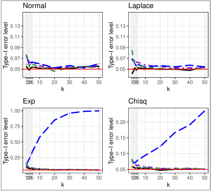
Figure 2: Type-I error simulation results ($\alpha=0.05$) of the tests $T_{W}^{*}$ $({\color[rgb]{0,0,0}\textendash\textendash\textendash})$, $T_{A}^{*}$ $({\color[rgb]{.75,.5,.25}\cdots})$, $T_{M}^{*}$ $({\color[rgb]{.5,0,.5}-\cdot-})$, $T_{NC}$ $({\color[rgb]{0,0,1}\textendash\textendash\quad\textendash\textendash})$, and $T_{LT}$ $({\color[rgb]{0,0,0}--})$, for different distributions under correlation factor ($\rho=0.9$) and heteroscedastic covariance matrix $\Sigma_{2}$ for varying $k$ values multiplied by $(n_{c},n_{u})=(10,30)$ under the MCAR framework.

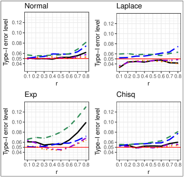
Figure 3: Type-I error simulation results ($\alpha=0.05$) of the tests $T_{W}^{*}$ $({\color[rgb]{0,0,0}\textendash\textendash\textendash})$, $T_{A}^{*}$ $({\color[rgb]{.75,.5,.25}\cdots})$, $T_{M}^{*}$ $({\color[rgb]{.5,0,.5}-\cdot-})$, $T_{NC}$ $({\color[rgb]{0,0,1}\textendash\textendash\quad\textendash\textendash})$, and $T_{LT}$ $({\color[rgb]{0,0,0}--})$, for different distributions under correlation factor ($\rho=0.5$) with sample size $(n=30)$ and homoscedastic covariance matrix $\Sigma_{1}$ for varying missing rates $r\in\{0.1,0.2,0.3,0.4,0.5,0.6,0.7,0.8\}$ under the MCAR framework.

7 Breast Cancer Study: Gene Expression Data

The Cancer Genome Atlas (TCGA) project is a pilot project which was launched in 2005 with a financial support from the National Institutes of Health. It aims to understand the genetic basis of several types of human cancers through the application of high-throughput genome analysis techniques. TCGA collects molecular information such as miRNA/mRNA expressions, protein expressions, weight of the sample as well as clinical data about the patients.

A breast cancer study has been performed by TCGA to improve the ability of diagnosing, treating and preventing breast cancer through investigating the genetic basis of carcinoma. Their study consists of $1093$ breast cancer patients with Clinical and RNA sequencing records. Among them, there were 112 subjects that provided both, normal and tumor tissues. Here, we were interested in a subset of this data that contains patients with pathologic stage I. This subset contains a total of $n_{c}=16$ complete pairs and an unpaired sample for the patients who developed only tumor tissues of size $n_{u}=74$. The data can be downloaded from Firehouse (www.gdac.broadinstitute.org).

Based on previous studies, six genes have been found to be significantly associated with breast cancer: TP53, ABCC1, HRAS, GSTM1, ERBB2 and CD8A.finak2008stromal ; harari2000molecular ; munoz2007role ; de2002genes Another two genes; C1D and GBP3 were under investigation although they did not show any significant relation towards breast cancer patients.qi2018testing In this paper, we aim to test the hypothesis whether mean genetic expressions of the eight genes are significantly different between normal and tumor tissues for patients with early stage I breast cancer. Boxplots representing the characteristics of the eight genes are shown in Figure 4.

We applied all bootstrap testing methods $T_{W}^{*},T_{A}^{*}$ and $T_{M}^{*}$ as well as the alternative approaches $T_{NC},T_{LT}$ to detect the null hypothesis of equal means between normal and tumor tissues $(H_{0}:\mu_{1}=\mu_{2})$ against the two-sided alternative $(H_{1}:\mu_{1}\neq\mu_{2})$. The results are summarized in Table 5.

It can bee seen from Table 5 that the bootstrapped approaches $T_{W}^{*},T_{A}^{*}$ and $T_{M}^{*}$ and Little’s method ($T_{LT}$) identified three out of eight genes having significantly different genetic expressions in normal and tumor tissues; genes ABCC1, HRAS, and ERBB2. However, the nonparametric combination method $T_{NC}$ led to different results for the ERBB2 gene.

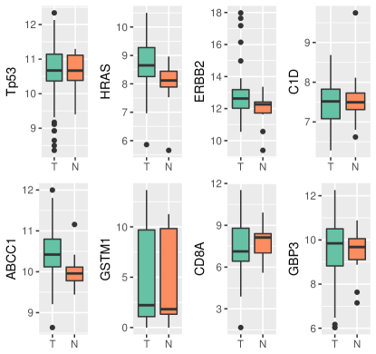
Figure 4: Profile of the Gene expression levels of the tumor and normal breast tissues

Table 5: Unadjusted two-sided P-values of the breast cancer study.

Gene	$\boldsymbol{T}_{\mathbf{W}}^{*}$	$\boldsymbol{T}_{\mathbf{A}}^{*}$	$\boldsymbol{T}_{\mathbf{M}}^{*}$	$\boldsymbol{T}_{\textbf{NC}}$	$\boldsymbol{T}_{\textbf{LT}}$
TP53	0.9120	0.8560	0.8990	0.9539	0.8804
ABCC1	0.0000	0.0010	0.0000	0.0030	0.0019
HRAS	0.0050	0.0010	0.0030	0.0011	0.0034
GSTM1	0.8080	0.8280	0.8300	0.6295	0.9202
ERBB2	0.0390	0.0350	0.0140	0.0712	0.0180
CD8A	0.4290	0.4800	0.4690	0.5545	0.4534
C1D	0.7900	0.5550	0.6360	0.5869	0.5097
GBP3	0.2030	0.2900	0.2270	0.1027	0.1294

8 Discussion and outlook

The problem of matched pairs with missing values occurs frequently in practice. Most available procedures in the literature are not applicable when missing values occur in a single arm. One exception is the recent NCT approach by Qi et al. qi2018testing who utilize a combination of the sign and Wilcoxon Mann-Whitney rank sum test. For homoscedastic settings with symmetric distributions, this approach can be recommended. If, however, the underlying assumptions are not true (e.g. in skewed heteroscedastic set-ups), the NCT may result in highly inflated type-I-errors or considerable power loss. To overcome these issues, we have provided resampling procedures that are not based on any parametric assumptions and use all observed information of the matched pairs design. They were shown to be asymptotically correct and robust under heteroscedasticity and skewed distributions. The tests were based on restructuring all observed information in a test statistic of quadratic form that can be either a Wald-type statistic (WTS), an ANOVA-type statistic (ATS), or a modified ANOVA-type statistic (MATS). Since WTS is well known (from other situations vallejo2010analysis ; konietschke2015parametric ; smaga2017bootstrap ) for being liberal, while ATS and MATS tend to be rather conservative or liberal for small to moderate sample sizes, we improved their small sample behavior by an asymptotic model based bootstrap approach. The procedure’s asymptotic validity was also proven.

In an extensive simulation study, the type-I error rate control of the tests have been examined for symmetric and skewed distributions with homoscedastic and heteroscedastic covariance settings under different missing mechanisms. There, it was seen that the parametric bootstrap versions of WTS, ATS, and MATS improve their small sample behaviour. In particular, our bootstrap tests have been shown to perform very well in most of the cases, even with larger amount of missingness, heteroscedastic covariance or skewed data. Only the type-I error control for the exponential distribution, particularly under heteroscedasticity, MCAR and small paired sample sizes with rather large unpaired portions $(n_{c}=10,n_{u}=30)$, is not maintained. In this setting, however, all other considered methods qi2018testing ; little1976inference also failed to control the type-I error rate. Regarding the individual performance of each bootstrapped test, the parametric bootstrap version of the ATS yielded the most robust results and is therefore recommended.

Furthermore, our simulation study exhibits that the bootstrap procedures’ type-I-error control is not much affected by less stringent missing data mechanism such as the MAR. However, their power behaviors is quite affected.

In order to simplify the application of our approaches, the three proposed bootstrap statistical methods have been implemented within the PBT function in the freely available R-package MissPair. It is available on GitHub (https://github.com/lubnaamro/MissPair) and will be available on the CRAN repository.

Future research will be concerned with extending our procedures to multivariate settings (MANOVA).

Burim Ramosaj and Markus Pauly acknowledge the support of the German Research Foundation (DFG). Lubna Amro’s work was also supported by the German Academic Exchange Service (DAAD) under the project: Research Grants - Doctoral Programmes in Germany, 2015/16 (No. 57129429).
Conflict of Interest: None declared.

Table 6: Power simulation results ($\alpha=0.05$) of the tests for different distributions under varying correlation values ($\rho$) with sample sizes $(n_{c},n_{u})=(30,10)$ and homoscedastic covariance matrix $\Sigma_{1}$ under the MCAR framework. Values of too liberal tests corresponding to red values in the $(30,10)-$column from Table 1 are printed in red colour.

Dist	$\rho$	$\delta=0.5$						$\delta=1$
		$T_{W}^{*}$	$T_{A}^{*}$	$T_{M}^{*}$	$T_{NC}$	$T_{LT}$		$T_{W}^{*}$	$T_{A}^{*}$	$T_{M}^{*}$	$T_{NC}$	$T_{LT}$
Normal	-0.9	24.7	34.1	32.1	32.1	35.7		76	86.4	84.2	82.6	87.9
	-0.5	28.7	36.9	36.2	34.9	40.1		84.1	90.6	90	87.3	92.5
	-0.1	35.6	40.2	42.5	40.5	48.7		92.5	94.1	95.4	92.4	97.2
	0.1	42.4	42.8	49.4	45.1	56.1		96.5	95.9	97.9	95.3	98.9
	0.5	64.7	44.6	68.9	58.1	78.1		99.9	98.1	100	99.1	100
	0.9	100	46.1	100	96.1	100		100	99.6	100	100	100
Laplace	-0.9	25.9	34.9	34.6	40.6	36.6		78.4	86.9	86	90.8	87.9
	-0.5	29.5	38.6	38.8	46.8	42		85.3	90.1	90.6	94.5	92.1
	-0.1	38.2	42.4	45.9	54.7	50.7		92.8	93.4	95.4	97.2	96.6
	0.1	44.2	44.2	51.6	59.1	57.5		95.9	94.5	97.4	98.4	98.3
	0.5	68.2	47.9	72	74.1	80		99.7	96.9	99.8	99.7	99.9
	0.9	99.9	49.4	99.9	97.9	99.3		100	98.7	100	100	100
Exp	-0.9	25.4	36	34.8	50.3	38.1		77.4	86.8	85.9	94.3	87.5
	-0.5	27.9	38.6	37	57.2	43.3		81.5	90.2	89	96.6	91.5
	-0.1	37.4	43.8	45	66.5	52.9		89.1	93.8	93.6	98.1	95.3
	0.1	42.2	44.5	48.9	70.4	58.6		93.3	95.4	95.9	98.8	97.2
	0.5	65.2	48.9	69	81.2	78.3		99.2	98.3	99.5	99.9	99.8
	0.9	99.8	51.1	99.7	98.1	98.5		100	99.7	100	100	100
Chisq	-0.9	23	33.1	30.5	31.8	34.9		75.6	85.9	84.1	83.3	87.3
	-0.5	28	37.1	35.6	36.6	41.2		83.7	90.8	89.8	88.4	92.6
	-0.1	34.3	39.9	41.8	41.1	49.4		92.1	94.7	95.3	93	97.3
	0.1	41.9	43.3	49	46.2	57		95.6	96.1	97.5	95.4	98.8
	0.5	65.7	45.8	69.9	60.7	79		99.8	98.6	99.9	99.1	100
	0.9	100	46	100	95.6	99.9		100	99.8	100	100	100

Table 7: Power simulation results ($\alpha=0.05$) of the tests for different distributions under varying correlation values ($\rho$) with sample sizes $(n_{c},n_{u})=(30,10)$ and heteroscedastic covariance matrix $\Sigma_{2}$ under the MCAR framework. Values of too liberal tests corresponding to red values in the $(30,10)-$column from Table 2 are printed in red colour.

Dist	$\rho$	$\delta=0.5$						$\delta=1$
		$T_{W}^{*}$	$T_{A}^{*}$	$T_{M}^{*}$	$T_{NC}$	$T_{LT}$		$T_{W}^{*}$	$T_{A}^{*}$	$T_{M}^{*}$	$T_{NC}$	$T_{LT}$
Normal	-0.9	17.8	25.6	23.6	21.7	26.3		58.8	72.3	69.1	65.0	73.1
	-0.5	19.9	27.3	26.1	23.4	28.7		66.3	78.2	76.0	70.0	79.4
	-0.1	24.4	30.7	30.8	26.8	34.1		76.4	83.8	83.8	77.5	87.4
	0.1	28.2	32.8	34.9	30.0	39.4		83.6	87.0	88.7	82.1	92.3
	0.5	42.9	35.0	48.1	38.3	56.7		96.6	91.4	97.7	91.6	98.9
	0.9	95.0	36.8	93.1	69.9	96.3		100.0	96.9	100.0	99.8	100.0
Laplace	-0.9	18.4	26.3	25.9	28.4	27.3		61.4	73.8	72.0	77.0	74.2
	-0.5	20.6	28.3	28.2	32.9	29.5		68.0	78.2	77.5	84.0	79.3
	-0.1	26.1	32.5	33.5	39.0	36.1		77.3	83.4	84.5	89.4	87.2
	0.1	29.1	33.8	36.6	42.5	41.2		83.7	86.1	88.6	92.4	91.1
	0.5	46.4	37.6	51.7	54.6	59.5		96.0	91.6	97.2	97.4	98.3
	0.9	93.7	38.5	91.6	84.5	92.9		100.0	95.7	100.0	99.9	100.0
Exp	-0.9	21.2	29.5	29.0	50.3	31.0		61.0	72.2	71.6	87.9	73.4
	-0.5	22.0	31.3	29.9	55.5	33.4		64.1	77.1	75.6	91.2	78.2
	-0.1	28.6	36.0	35.8	63.2	40.7		73.0	82.2	81.5	93.8	84.2
	0.1	31.2	36.2	37.5	66.0	43.4		79.0	84.8	85.2	95.4	88.1
	0.5	47.7	39.7	51.4	74.3	59.0		92.8	90.4	93.8	98.2	96.4
	0.9	90.4	41.3	86.7	89.5	88.6		100.0	95.5	99.9	99.9	99.5
Chisq	-0.9	17.8	25.4	23.2	24.9	26.1		57.9	72.3	69.1	68.1	73.2
	-0.5	20.3	28.7	26.9	28.3	30.3		65.4	78.6	75.9	74.4	79.6
	-0.1	23.7	30.6	30.2	31.2	35.0		75.3	84.0	83.4	80.9	87.0
	0.1	29.0	33.9	35.6	35.5	41.2		81.5	86.5	87.6	84.8	90.7
	0.5	44.6	36.1	49.6	45.4	58.0		95.8	91.9	96.9	93.2	98.4
	0.9	93.5	36.8	90.6	73.6	94.4		100.0	96.8	100.0	99.8	100.0

Table 8: Power simulation results ($\alpha=0.05$) of the tests for different distributions under varying correlation values ($\rho$) with sample sizes $n=20$ and homoscedastic covariance matrix $\Sigma_{1}$ under the MAR framework. Values of too liberal tests corresponding to red values in the $(n=20)-$column from Table 3 are printed in red colour.

Dist	$\rho$	$\delta=0.5$						$\delta=1$
		$T_{W}^{*}$	$T_{A}^{*}$	$T_{M}^{*}$	$T_{NC}$	$T_{LT}$		$T_{W}^{*}$	$T_{A}^{*}$	$T_{M}^{*}$	$T_{NC}$	$T_{LT}$
Normal	-0.9	11.6	18.8	17.4	17.2	19.4		35.7	55.8	49.7	52.6	57.8
	-0.5	14.3	20.5	20.1	20	22.9		43.6	60.2	56.4	56.6	64.8
	-0.1	17.2	20.7	22	21.4	26.6		55.6	64.7	65.5	63.7	75.4
	0.1	20.6	21.9	25	24.4	32.2		63.6	67.1	71.9	68.8	82
	0.5	31.9	20.8	35	30.4	47.2		88	72	90.5	82.1	95.8
	0.9	93.1	19.9	92.8	68.8	93.3		100	75	100	98.9	100
Laplace	-0.9	12.7	20.9	21.8	22.6	22		40.9	58.6	56.1	61.7	59.4
	-0.5	14.3	21.6	22.9	25.5	23.8		48.8	63.1	62.8	69	66.3
	-0.1	18.1	23.6	25.9	30.5	29.4		60.4	68.9	71.1	76.6	76.6
	0.1	21.5	24.8	28.3	33.5	33.9		67.8	71.3	76	80.2	81.8
	0.5	35.4	25.6	38.8	42.5	50.5		87.9	76.7	90.3	89.7	95
	0.9	91.6	22.3	90.7	74.4	89.6		100	79.1	100	99.1	99.6
Exp	-0.9	11.1	21.8	22.6	26.8	22.4		41.9	61	60.7	69.2	62.5
	-0.5	14.2	24.5	22.6	31.4	26.8		45.6	66.9	65.4	74	68.9
	-0.1	18.6	25.2	23.6	36.7	33		57.1	72	71	79.9	76.5
	0.1	22.4	25.6	25.8	38.4	37.4		64.5	75	75.4	83.4	82.1
	0.5	35.1	23.4	35.1	44	51.8		85.2	80.4	87.6	89.9	93.8
	0.9	91.5	17.5	87.6	71.2	88.8		100	85.2	100	99.4	99.2
Chisq	-0.9	11.7	19.1	18.1	17.8	19.6		34.8	56.7	50.7	53.2	58
	-0.5	13.2	19.9	18.7	19.1	22.3		42.4	60.2	56.3	57	64.8
	-0.1	16.7	20.6	21.2	21.3	27.8		54.9	66.6	66	64.7	76.1
	0.1	19.6	20.8	23.3	23.3	31.5		63.5	69.4	72.4	68.8	82.1
	0.5	31.8	20.4	33.8	31.2	47.8		87.1	73.8	89.6	81.5	95.4
	0.9	92.2	17.2	91.9	65.4	93.1		100	78.1	100	98.9	100

Table 9: Power simulation results ($\alpha=0.05$) of the tests for different distributions under varying correlation values ($\rho$) with sample sizes $n=20$ and heteroscedastic covariance matrix $\Sigma_{2}$ under the MAR framework. Values of too liberal tests corresponding to red values in the $(n=20)-$column from Table 4 are printed in red colour.

Dist	$\rho$	$\delta=0.5$						$\delta=1$
		$T_{W}^{*}$	$T_{A}^{*}$	$T_{M}^{*}$	$T_{NC}$	$T_{LT}$		$T_{W}^{*}$	$T_{A}^{*}$	$T_{M}^{*}$	$T_{NC}$	$T_{LT}$
Normal	-0.9	9.9	16	15.8	13.2	15.8		24.7	42.5	37.7	37	43.4
	-0.5	10.8	15.9	16.4	13.7	16.6		29.7	46.4	43.5	40.8	48.7
	-0.1	12.6	16.1	16.8	14.8	19.5		36.8	49.3	48.7	44.6	56.2
	0.1	14.1	16.6	18.2	16.3	22.1		44.5	52.2	54.5	48.7	63.5
	0.5	20.9	16.6	23.9	19.4	31.9		66.4	56.7	71.2	60.1	82.9
	0.9	61.5	14.5	53.1	33.1	74.5		99.7	58.1	99.2	88.6	99.2
Laplace	-0.9	10.2	16	17.9	16.2	16.4		27.6	45	42.9	45.9	45.4
	-0.5	11.3	17.3	18.9	19.1	18.3		34.3	48.9	48.9	53.4	50
	-0.1	12.6	18.4	20.2	21.8	21.4		43.2	55	56.2	60.5	60.2
	0.1	14.7	18.6	21	23	24.3		47.9	56.4	59.5	63.1	65.4
	0.5	23.3	19.3	26.7	28.3	36.3		68.1	60.1	73	72.4	82.5
	0.9	64.2	16.5	57.6	46.8	74.3		98.9	62.2	97.8	91.3	97
Exp	-0.9	11.5	19.9	22.6	27.6	20.2		33.2	48.7	49.8	57.7	49.4
	-0.5	13.7	22.1	22.6	30.7	23.2		34.7	53.4	53.9	62.2	54.4
	-0.1	18	23.5	23.2	34.5	27.6		43	56.8	57	67.3	60.3
	0.1	19.9	22.6	23.4	34.9	29.5		48.9	59	60.3	70.1	65.2
	0.5	29.8	21.3	29.7	38.6	39.7		66.5	61.7	69.4	75.7	79.1
	0.9	66.5	15.2	54.2	49.9	72.9		97.2	63.5	93.9	90.4	93.8
Chisq	-0.9	9.5	15.5	15.1	14.4	15.8		25.6	43.2	39.4	39.7	44.1
	-0.5	11	16.5	16.3	15.6	17.3		30.5	47.1	44.2	43.3	49.1
	-0.1	13	16.6	17.2	17	21.1		38.4	51.5	50.9	49.1	57.9
	0.1	15.1	17.3	18.6	17.9	23.6		44.5	52.9	55	51.6	63.8
	0.5	22.6	16.5	24.3	22.3	33.7		65.6	56.5	69.4	61.1	81.4
	0.9	63.3	13.2	53.4	35.7	73.9		99.3	59	98	85.7	98.5

References

- (1) Kuriakose MA, Chen WT, He Z et al. Selection and validation of differentially expressed genes in head and neck cancer. Cell Mol Life Sci 2004; 61: 1372–1383.
- (2) Lapointe J, Li C, Higgins JP et al. Gene expression profiling identifies clinically relevant subtypes of prostate cancer. Proc Natl Acad Sci U S A 2004; 101: 811–816.
- (3) Feng Q, Hawes SE, Stern JE et al. DNA methylation in tumor and matched normal tissues from non-small cell lung cancer patients. Cancer Epidemiol Biomark Prev 2008; 17: 645–654.
- (4) Schafer JL. Multiple imputation: a primer. Stat Methods Med Res 1999; 8(1): 3–15.
- (5) Rubin DB. Multiple imputation for nonresponse in surveys. New York: Wiley, 2004.
- (6) Sterne JA, White IR, Carlin JB et al. Multiple imputation for missing data in epidemiological and clinical research: potential and pitfalls. Bmj 2009; 338: b2393.
- (7) Stekhoven DJ and Bühlmann P. MissForest: non-parametric missing value imputation for mixed-type data. Bioinformatics 2011; 28(1): 112–118.
- (8) Waljee AK, Mukherjee A, Singal AG et al. Comparison of imputation methods for missing laboratory data in medicine. BMJ open 2013; 3(8): e002847.
- (9) Ramosaj B and Pauly M. Predicting missing values: a comparative study on non-parametric approaches for imputation. Comput Stat 2019; 34(4): 1741–1764.
- (10) Ramosaj B, Amro L and Pauly M. A cautionary tale on using imputation methods for inference in matched pairs design. Arxiv pre-print 2018; .
- (11) Van Buuren S. Flexible imputation of missing data. Chapman and Hall/CRC, 2018.
- (12) Mehta J and Gurland J. Testing equality of means in the presence of correlation. Biometrika 1969; 56: 119–126.
- (13) Lin PE. Procedures for testing the difference of means with incomplete data. J Am Stat Assoc 1973; 68: 699–703.
- (14) Morrison DF. A test for equality of means of correlated variates with missing data on one response. Biometrika 1973; 60: 101–105.
- (15) Lin PE and Stivers LE. On difference of means with incomplete data. Biometrika 1974; 61: 325–334.
- (16) Little RJ. Inference about means from incomplete multivariate data. Biometrika 1976; 63: 593–604.
- (17) Ekbohm G. On comparing means in the paired case with incomplete data on both responses. Biometrika 1976; 63: 299–304.
- (18) Bhoj DS. Testing equality of means of correlated variates with missing observations on both responses. Biometrika 1978; 65: 225–228.
- (19) Looney SW and Jones PW. A method for comparing two normal means using combined samples of correlated and uncorrelated data. Stat Med 2003; 22: 1601–1610.
- (20) Kim BS, Kim I, Lee S et al. Statistical methods of translating microarray data into clinically relevant diagnostic information in colorectal cancer. Bioinformatics 2005; 21: 517–528.
- (21) Samawi HM and Vogel R. Notes on two sample tests for partially correlated (paired) data. J Appl Stat 2014; 41: 109–117.
- (22) Uddin N and Hasan M. Testing equality of two normal means using combined samples of paired and unpaired data. Commun Stat Simul Comput 2017; 46: 2430–2446.
- (23) Amro L and Pauly M. Permuting incomplete paired data: A novel exact and asymptotic correct randomization test. J Stat Comput Sim 2017; 87: 1148–1159.
- (24) Amro L, Konietschke F and Pauly M. Multiplication-combination tests for incomplete paired data. Stat Med 2019; 38: 3243–3255.
- (25) Qi Q, Yan L and Tian L. Testing equality of means in partially paired data with incompleteness in single response. Stat Methods Med Res 2018; 28: 1508–1522.
- (26) Rempala GA and Looney SW. Asymptotic properties of a two sample randomized test for partially dependent data. J Stat Plan Inference 2006; 136: 68–89.
- (27) Samawi HM, Helu A and Vogel R. A nonparametric test of symmetry based on the overlapping coefficient. J Appl Stat 2011; 38: 885–898.
- (28) Yu D, Lim J, Liang F et al. Permutation test for incomplete paired data with application to cDNA microarray data. Comput Stat Data Anal 2012; 56: 510–521.
- (29) Kuan PF and Huang B. A simple and robust method for partially matched samples using the p-values pooling approach. Stat Med 2013; 32: 3247–3259.
- (30) Krishnamoorthy K and Lu F. A parametric bootstrap solution to the MANOVA under heteroscedasticity. J Stat Comput Simul 2010; 80: 873–887.
- (31) Xu LW, Yang FQ, Qin S et al. A parametric bootstrap approach for two-way ANOVA in presence of possible interactions with unequal variances. J Multivar Anal 2013; 115: 172–180.
- (32) Konietschke F, Bathke AC, Harrar SW et al. Parametric and nonparametric bootstrap methods for general MANOVA. J Multivar Anal 2015; 140: 291–301.
- (33) Friedrich S and Pauly M. MATS: Inference for potentially singular and heteroscedastic MANOVA. J Multivar Anal 2018; 165: 166–179.
- (34) Vallejo G, Fernández M and Livacic-Rojas PE. Analysis of unbalanced factorial designs with heteroscedastic data. J Stat Comput Simul 2010; 80(1): 75–88.
- (35) Smaga Ł. Bootstrap methods for multivariate hypothesis testing. Commun Stat - Simul Comput 2017; 46: 7654–7667.
- (36) Brunner E. Asymptotic and approximate analysis of repeated measures designs under heteroscedasticity. Mathematical Statistics with Applications in Biometry 2001; 313–326.
- (37) Ekbohm G. On comparing means in the paired case with incomplete data on both responses. Biometrika 1976; 63: 299–304.
- (38) Mehta J and Gurland J. A test for equality of means in the presence of correlation and missing values. Biometrika 1973; 60: 211–213.
- (39) Finak G, Bertos N, Pepin F et al. Stromal gene expression predicts clinical outcome in breast cancer. Nat Med 2008; 14: 518–527.
- (40) Harari D and Yarden Y. Molecular mechanisms underlying ErbB2/HER2 action in breast cancer. Oncogene 2000; 19: 6102–6114.
- (41) Munoz M, Henderson M, Haber M et al. Role of the MRP1/ABCC1 multidrug transporter protein in cancer. IUBMB life 2007; 59: 752–757.
- (42) De Jong M, Nolte I, Te Meerman G et al. Genes other than BRCA1 and BRCA2 involved in breast cancer susceptibility. J Med Genet 2002; 39: 225–242.