AdS₅–Schwarzschild deformed black branes and hydrodynamic transport coefficients

Abstract

A family of deformed AdS₅–Schwarzschild black branes is here derived, employing the membrane paradigm of AdS/CFT. The solution of the Einstein–Hilbert action, with the Gibbons–Hawking term and a counter-term that eliminates eventual divergences, yields a partition function associated to the dual theory which allows the computation of the entropy, pressure and free energy, as state functions, in the canonical ensemble. AdS/CFT near-horizon methods are then implemented to compute the shear viscosity-to-entropy ratio, then restricting the range of the parameter that defines a family of deformed black branes.

I Introduction

AdS/CFT is a paradigm relating gravity in anti-de Sitter (AdS) spacetime to a large-$N$ conformal field theory (CFT), located on the AdS codimension-1 boundary. Perturbatively, considering an $1/N$ expansion, quantum fields in the bulk correspond to CFT operators rangamani ; minwalla ; hubeny_hard . The dynamics of Einstein’s equations, describing weakly coupled gravity in an AdS space, rules the corresponding dynamics of the energy-momentum tensor of strongly coupled QFTs on the AdS boundary. In the $N\to\infty$ t’ Hooft regime, keeping a fixed coupling, the gauge theory on the boundary is an effective classical theory.

The AdS boundary is usually identified to a 4D brane. Braneworld models describe a brane that has tension, $\sigma$, constrained to both the bulk and the brane cosmological constants Casadio:2015gea ; daRocha:2017cxu . General relativity (GR) describes gravity in an infinitely rigid brane, with an infinite tension. However, recent works derived a strong bound for the finite brane tension, lying in the bound $\sigma\gtrsim 2.81\times 10^{-6}\;{\rm GeV^{4}}$ Casadio:2016aum ; Fernandes-Silva:2019fez . This condition in fact produces a physically correct low energy limit, allowing the construction of an AdS/CFT membrane paradigm analogue of any classical GR solution ads_memb ; first ; mgd1 ; mgd2 ; daRocha:2017cxu ; Casadio:2015gea ; maartens . One can also describe the AdS bulk gravity by a black hole, which behaves as a fluid at its own horizon, in the membrane paradigm. Einstein’s equations near the horizon of the black hole reduce to the Navier-Stokes equations for the fluid rangamani ; minwalla ; hubeny_hard . A fluid at the black hole horizon mimics a fluid at the AdS boundary Eling:2009sj ; Antoniadis:1990ew ; Antoniadis:1998ig ; ads_memb , introducing an useful dictionary, linking brane models and the membrane paradigm of AdS/CFT. Here we aim to derive new deformed asymptotically AdS black branes and use the shear viscosity-to-entropy density ratio, $\frac{\eta}{s}$, and the deformed black brane temperature, to impose viscosity bounds to the free parameter in these new solutions. In the context of AdS/CFT correspondence, a precise relationship between the gravitational result and the dual field theory is then established, and further discussed.

In AdS/CFT, the AdS₅-Schwarzschild black brane is dual to the gauge theory describing the strongly-coupled, large-$N_{c}$, $\mathcal{N}=4$, plasma. In this scheme, the famous ratio $\frac{\eta}{s}=\frac{1}{4\pi}$ (and the conjectured KSS bound) is obtained, which is indeed a quite small value, compared to ordinary materials. However, if large-$N_{c}$ gauge theories considered by AdS/CFT are good approximations to QCD, one could expect that this result may be applied to the quark-gluon plasma (QGP) qgp . In fact, experiments in the Relativistic Heavy Ion Collider (RHIC) have shown that the QGP behaves like a viscous fluid with very small viscosity, which implies that the QGP is strongly-coupled, which discards the possibility of using perturbative QCD to the study of the plasma qgp_exps . Thus, AdS/CFT may present itself as an alternative to the QGP research and generalizations thereof qgpexp1 ; qgpexp2 .

Previously, we have explored the technique employed here to derive a family of solutions that consists of a deformation in the AdS₄–Reissner–Nordström background, and its potential applications to AdS/CMT Ferreira-Martins:2019wym . By embedding the brane into a higher dimensional bulk, we were able to mimic the Hamiltonian and momentum constrains from the ADM formalism for static configurations of the metric field Casadio:2001jg ; Abdalla:2006qj . These equations turn out to be a weaker condition on the metric functions, allowing for a family of deformations of solutions from classical GR. In the present work we apply a similar procedure to the AdS₅–Schwarzschild black brane BoschiFilho:2004ci ; BoschiFilho:2003zi .

The paper is organized as follows: in Sect. II the relevant results of linear response theory and fluid dynamics are briefly presented within the hydrodynamics formalism, followed by a presentation of the AdS/CFT duality. Sect. III is then devoted to derive the AdS₅–Schwarzschild deformed gravitational background. The solution of the Einstein–Hilbert action, also containing the Gibbons–Hawking term and a counter-term that precludes divergences, yields a partition function for the dual theory. Hence, entropy, pressure and free energy, are computed as state functions, in the canonical ensemble. The explicit computation of the $\frac{\eta}{s}$ ratio is carried out for the family AdS₅–Schwarzschild deformed black branes in Sect. IV. The saturation of $\frac{\eta}{s}$ and the black brane temperature therefore is shown to constrain the free parameter AdS₅–Schwarzschild deformed black brane, driving the family of deformed branes to two unique solutions: the standard AdS₅–Schwarzschild black brane and a new black brane solution. The concluding remarks are then presented in Sect. VI.

II Hydrodynamics and linear response theory

The so called hydrodynamic limit is characterized by the long-wavelength, low-energy regime Rangamani:2009xk , and is often applicable to describe conserved quantities. As an effective description of field theory, hydrodynamics naturally does not contain the details of a microscopic theory. These are encoded into the transport coefficients, among which the shear viscosity, $\eta$, plays a prominent role.

The macroscopic variables encoded in the energy-momentum stress tensor, $T^{\mu\nu}$, along with its conservation law, $\partial_{\mu}T^{\mu\nu}=0$, describe a simple fluid. In general, one introduces a constitutive equation by determining the form of $T^{\mu\nu}$ in a derivative expansion, given in terms of the normalized fluid velocity field $u^{\mu}(x^{\nu})$, its pressure field $p(x^{\mu})$ and its rest-frame energy density $\rho(x^{\mu})$.

To first order in the derivative expansion, the stress tensor is expressed as Rangamani:2009xk ; hubeny_hard

$$T^{\mu\nu}=p\left(\eta^{\mu\nu}+u^{\mu}u^{\nu}\right)+\rho u^{\mu}u^{\nu}+\tau^{\mu\nu}\ ,$$ (1)

where $\tau^{\mu\nu}$, the term which is first-order in derivatives, carries dissipative effects. The constitutive equation for a viscous fluid, as defined above, yields both the continuity and Navier–Stokes equations. For a theory described by an action functional $S$, the coupling of an operator $\mathcal{O}$ to an external source $\upvarphi^{(0)}$ reads son_hydro

$$S\mapsto S+\int\mathrm{d}^{4}x\upvarphi^{(0)}(t,\bm{x})\mathcal{O}(t,\bm{x})\ .$$ (2)

One is often interested in determining the response in $\mathcal{O}$, which, up to first order in $\upvarphi^{(0)}$, is known as linear response theory. The one-point function reads son_hydro

$$\updelta\left\langle\mathcal{O}(\omega,\bm{\mathfrak{q}})\right\rangle=-G_{R}^{\mathcal{O},\mathcal{O}}(\omega,\bm{\mathfrak{q}})\upvarphi^{(0)}(\omega,\bm{\mathfrak{q}})\ ,$$ (3)

where $G_{R}^{\mathcal{O},\mathcal{O}}(\omega,\bm{\mathfrak{q}})$ is the retarded Green’s function natsuume . The response of $\tau^{\mu\nu}$ under gravitational fluctuations is determined by an off-diagonal perturbation term, $h_{xy}^{(0)}$, leading to the perturbed metric minwalla ; hubeny_hard :

$$g_{\mu\nu}^{(0)}\mathrm{d}x^{\mu}\mathrm{d}x^{\nu}=\eta_{\mu\nu}\mathrm{d}x^{\mu}\mathrm{d}x^{\nu}+2h_{xy}^{(0)}(t)\mathrm{d}x\mathrm{d}y,$$ (4)

yielding the response son_hydro

$$\updelta\left\langle\tau^{xy}(\omega,\bm{\mathfrak{q}}=\bm{0})\right\rangle=i\omega\eta h_{xy}^{(0)}=-G_{R}^{xy,xy}h_{xy}^{(0)}\ .$$ (5)

and the Kubo formula

$$\eta=-\lim_{\omega\rightarrow 0}\frac{1}{\omega}\operatorname{Im}\left(G_{R}^{xy,xy}(\omega,\bm{0})\right).$$ (6)

Computation of the retarded Green’s function is straightforwardly achieved, once the GKPW relation gkp1 ; gkp2 is regarded. It yields the following expression for the one-point function, gkp2 ; Witten:1998qj ,

$$\left\langle\mathcal{O}\right\rangle_{S}=\frac{\updelta\bar{S}[\upvarphi^{(0)}]}{\updelta\upvarphi^{(0)}}\ .$$ (7)

One considers the bulk theory to be GR, with negative cosmological constant, $\Lambda_{5}$. Therefore the action reads

$$S=\frac{1}{16\pi}\int d^{5}x\sqrt{-g}\left(R-2\Lambda_{5}\right)+S_{mat}\ ,$$ (8)

where $S_{mat}$ is specified by the boundary theory of interest. The action for massless scalar field is just a kinetic term. A particular case of interest is the AdS₅–Schwarzschild spacetime,

$$ds^{2}=-\frac{r_{0}^{2}}{u^{2}}f(u)\mathrm{d}t^{2}+\frac{1}{u^{2}f(u)}\mathrm{d}u^{2}+\frac{r_{0}^{2}}{u^{2}}\delta_{ij}\mathrm{d}x^{i}\mathrm{d}x^{j}\ ,$$ (9)

where $f(u)=1-u^{4}$, with $u=r_{0}/r$ defining the radial coordinate hereon in this paper, where $r_{0}$ is the horizon radius. Hence $u=1$ locates the horizon, whereas $u=0$ is the spacetime boundary. For $u\rightarrow 0$, Eq. (9) reads

$$ds^{2}=\frac{r_{0}^{2}}{u^{2}}\left(-\mathrm{d}t^{2}+\frac{1}{r_{0}^{2}}\mathrm{d}u^{2}+\delta_{ij}\mathrm{d}x^{i}\mathrm{d}x^{j}\right)\ .$$ (10)

The one-point function, Eq. (7), depends only on the matter contribution when computing the on-shell action. Assuming $\upvarphi=\upvarphi(u)$, and denoting by a dot the derivative with respect to $u$, the action for the massless scalar field at the boundary becomes

$$\!\!\!\!\!\!\!\!\!\!\!S\!\sim\!\int\!\mathrm{d}^{4}x\!\left.\left(\frac{r_{0}^{4}}{2u^{3}}\upvarphi\dot{\upvarphi}\right)\right\rvert_{u=0}\!\!\!\!\!+\int\mathrm{d}^{5}x\!\left(\frac{r_{0}^{4}}{2u^{3}}\ddot{\upvarphi}\!-\!\frac{3r_{0}^{4}}{2u^{4}}\dot{\upvarphi}\right)\!\upvarphi.$$ (11)

Eq. (11) is just the EOM for the scalar field, whose asymptotic solution reads

$$\upvarphi\sim\upvarphi^{(0)}\left(1+\upvarphi^{(1)}u^{4}\right)\ .$$ (12)

The on-shell action reduces to the surface term on the AdS boundary. Substituting the asymptotic form of the scalar field, Eq. (12) into Eq. (11) yields

$$\left\langle\mathcal{O}\right\rangle_{S}=4r_{0}^{4}\upvarphi^{(1)}\upvarphi^{(0)}=\updelta\left\langle\mathcal{O}\right\rangle.$$ (13)

Relating this result to Eq. (3) determines the retarded Green’s function,

$$G_{R}^{\mathcal{O},\mathcal{O}}(\bm{\mathfrak{q}}=\bm{0})=-4r_{0}^{4}\upvarphi^{(1)}.$$ (14)

III The AdS₅–Schwarzschild deformed black brane

The general solution to 5D vacuum Einstein gravity with a negative cosmological constant depends on the horizon metric $H_{ij}$ and an integration constant, $k$. Provided that the constraint $R_{ij}=3kH_{ij}$ holds, the solution for $k=0$, leading to a planar horizon i.e. $H_{ij}=\delta_{ij}$, is the AdS₅–Schwarzschild black brane Aminneborg:1996iz . The dual theory is a conformal fluid Bilic:2014dda . Hence its stress-energy tensor is traceless, fixing the bulk viscosity rangamani ; hubeny_hard , $\zeta=0$, leaving the shear viscosity $\eta$ as the only non-trivial transport coefficient son_hydro ; Son:2009zzc . We will present the arguments and a similar calculation, when considering the deformed AdS₅–Schwarzschild black brane as the gravitational background. The saturation of the $\frac{\eta}{s}$ ratio in the AdS₅–Schwarzschild black brane gravitational background reads kss

$$\frac{\eta}{s}=\frac{1}{4\pi}.$$ (15)

One does not need discuss specific bulk features, as the existence of solutions to the higher-dimensional Einstein’s equations describing gravity is undertaken by the Campbell–Magaard embedding theorems Bronnikov:2003gx .

There is a correspondence between AdS/CFT and braneworld scenarios. In an AdS bulk with cosmological constant $\Uplambda$, a solution must satisfy the effective Einstein’s equations

$$R_{AB}=\Uplambda\,g_{AB}+\mathcal{E}_{AB}\,,$$ (16)

where $A,B=0,1,2,3,5,6$. One can project Eq. (16) onto a timelike, codimension-1, embedding AdS manifold, in Gaussian coordinates $x^{M}$ = ($x^{\mu},x^{5}$) – for $\mu=0,1,2,3$, where $x^{5}=r$. When $r=0$, it corresponds to the brane itself, requires the Gauss–Codazzi equations to represent the embedding bulk Ricci tensor, when the discontinuity of the extrinsic curvature is related to the embedding codimension-1 bulk stress-tensor. Hence, the field equations yield the effective Einstein’s field equations on the bulk, whose corrections consist of an AdS bulk Weyl fluid ssm1 . This fluid flow is implemented by the bulk Weyl tensor, whose projection, the so called electric part of the Weyl tensor, reads

$$\!\!\!\!\!\!\!\!\mathcal{E}_{MN}(\sigma^{-1})\! = \!-\frac{6}{\sigma}\!\left[\mathcal{U}\!\left(\!u_{M}u_{N}\!+\!\frac{1}{3}h_{MN}\!\right)\!\right.$$ (17)

$$\left.\qquad\quad+\mathit{Q}_{(M}u_{N)}\!+\!\mathcal{P}_{MN}\right],$$

for $M,N=0,1,2,3,5$, where $h_{MN}$ denotes the projector operator that is orthogonal to the velocity, $u^{M}$, associated to the Weyl fluid flow. In addition, $\mathcal{U}=-\frac{1}{6}\sigma\mathcal{E}_{MN}u^{M}u^{N}$ is the effective energy density; $\mathcal{P}_{MN}=-\frac{1}{6}\sigma\left(h_{(M}^{\;P}h_{N)}^{\;Q}-\frac{1}{3}h^{PQ}h_{MN}\right)\mathcal{E}_{PQ}$ is the effective non-local anisotropic stress-tensor; and the effective non-local energy flux, $\mathit{Q}_{M}=-\frac{1}{6}\sigma h^{\;P}_{\mu}\mathcal{E}_{PN}u^{M}$, is originated from the bulk free gravitational field. The tension is described by $\sigma$. Local corrections are encoded into the tensor ssm1 ; Shiromizu:2001jm :

$$\!\!\!S_{MN}\!=\!\frac{T}{3}T_{MN}\!-\!T_{MP}T^{P}_{\ N}\!+\!\frac{g_{MN}}{6}\Big{[}3T_{PQ}T^{PQ}-T^{2}\Big{]}$$ (18)

where $T_{MN}$ is the matter stress-tensor and $T=T^{M}_{\;M}$ denotes the trace of $T_{MN}$. The trace of $S_{MN}$ corresponds to the trace anomaly of the cutoff CFT on the brane maartens . Higher-order terms in Eq. (18) are neglected, as the embedding bulk matter density is negligible. Denoting by $G_{MN}$ the Einstein tensor, the 5D Einstein’s effective field equations read

$$G_{MN}=T_{MN}+\mathcal{E}_{MN}(\sigma^{-1})+{\color[rgb]{0,0,0}\frac{1}{4\sigma}S_{MN}}=0.$$ (19)

Since $\mathcal{E}_{MN}\sim\sigma^{-1}$, it is straightforward to notice that in the infinitely rigid limit, $\sigma\rightarrow\infty$, GR is recovered and the Einstein’s field equations have the standard form $G_{MN}=T_{MN}$. Alternatively, the system of equations below is weaker than the effective field equations, and can be seen as constraints

$$R_{Mw}=0,\ \ \ \mathring{R}=\Lambda,$$ (20)

where ${\color[rgb]{0,0,0}w=x^{6}}$ is the bulk extra dimension; $\mathring{R}$ and $\Lambda$ denote, respectively, the codimension-1 embedding bulk Ricci scalar and the 5D cosmological constant. Eqs. (20) mimic constraints in the ADM procedure adm , whereas the equation $R_{MN}=\mathcal{E}_{MN}$ completes this system.

One supposes a general metric, setting the AdS radius to unity,

$$\!\!\!\!\!\!\!\!\!\!ds^{2}=-{r^{2}}N(r)\mathrm{d}t^{2}+\frac{1}{r^{2}A(r)}\mathrm{d}r^{2}+{r^{2}}\updelta_{ij}\mathrm{d}x^{i}\mathrm{d}x^{j}.$$ (21)

​By demanding that the ADM constraint leads to the AdS₅–Schwarzschild metric when $\beta\to 1$, and denoting by a prime the derivative with respect to $r$, the Hamiltonian constraint reads,

$${2N^{\prime\prime}(r)\over N(r)}-{N^{\prime 2}(r)\over N^{2}(r)}+{2A^{\prime\prime}(r)\over A(r)}+{A^{\prime 2}(r)\over A^{2}(r)}-{N^{\prime}(r)A^{\prime}(r)\over N(r)A(r)}$$

$$\quad+{4\over r}\,\left({N^{\prime}(r)\over N(r)}-{A^{\prime}(r)\over A(r)}\right)-{4A(r)\over r^{2}}=f(r,r_{0},\beta),$$ (22)

where the function $f(r,r_{0},\beta)$ is given by Eq. (80) in the Appendix A.

In the $u$ variable, the metric (21) reads

$$\!\!\!\!\!\!\!\!\!ds^{2}=-\frac{r_{0}^{2}}{u^{2}}N(u)\mathrm{d}t^{2}+\frac{1}{u^{2}A(u)}\mathrm{d}u^{2}+\frac{r_{0}^{2}}{u^{2}}\updelta_{ij}\mathrm{d}x^{i}\mathrm{d}x^{j},$$ (23)

The constraint (III) is satisfied by

$$N(u) = 1-u^{4}+\left(\beta-1\right)u^{6},$$ (24)

$$A(u) = \left(1-u^{4}\right)\left(\frac{2-3u^{4}}{2-\left(4\beta-1\right)u^{4}}\right).$$ (25)

The constant $\beta$ parameter is referred to as a deformation parameter. In the next section we will investigate how the shear-viscosity-to-entropy density ratio can drive specific values for $\beta$.

III.1 Thermodynamics

Combining the metric (23), with coefficients (24, 25), and the GKPW relation Witten:1998qj ; gkp2 , we are able to obtain the partition function associated to the dual theory, and calculate the thermodynamic functions such as entropy, pressure and free energy. Basically, the following action must be evaluated

$$\begin{aligned} S_{E}\!=\!-\frac{1}{16\pi G}&\!\overbrace{\int\!d^{5}x\sqrt{g}\left(R\!-2\!\Lambda_{5}\right)}^{I_{\rm bulk}}\!\\ &-\!\frac{1}{8\pi G}\overbrace{\lim_{u\to 0}\int\!d^{4}x\sqrt{h}K}^{I_{GH}}\!+\!I_{\text{c.t}}\ ,\end{aligned}$$ (26)

where the first term is the Einstein–Hilbert action with the cosmological constant, the second term is the Gibbons–Hawking term, and the last is the counter term, which is introduced to ensure that the result is finite. In this case one uses the Euclidean signature, obtained by performing a Wick rotation in the time coordinate $t\mapsto i\tau$. This implies that $\tau$ is a periodic coordinate with period $2\pi$ Wald:1995yp .

Each term will be individually computed, starting by the Einstein–Hilbert term. The cosmological constant is $-2\Lambda_{5}=12$, and the expansion on $u$ of the scalar curvature reads

$$R=-20-8\left(\beta-1\right)u^{4}+\ldots\ ,$$ (27)

since the variable $u$ is defined from $0$ to $1$. For the metric determinant, the expansion on $u$ is given by

$$\!\!\sqrt{g} \approx \frac{r_{0}^{4}}{u^{5}}-\frac{\left(\beta-1\right)r_{0}^{4}}{u}+\frac{1}{2}(\beta-1)r_{0}^{4}u$$ (28)

$$+\frac{\left(1-\beta\right)}{4}\left[6-\left(1-\beta\right)\right]r_{0}^{4}u^{3}.$$

Hence, the Einstein–Hilbert term becomes

$$\begin{aligned} \!\!\!\!I_{\text{bulk}}&=\left[\left(\frac{1}{\epsilon^{4}}-1\right)-2(\beta-1)\right.\\ &\left.+\frac{1}{2}\left(\beta^{2}+2(\beta-1)^{2}+\beta-2\right)\right]\!,\end{aligned}$$ (29)

where $\epsilon\to 0$ is used to keep track of divergent terms, which will be cancelled with the counter term.

The Gibbons–Hawking term is a surface term. By considering the normal vector $n_{\alpha}=g_{uu}^{-1/2}\delta_{\alpha}^{u}$, the induced metric for a hypersurface at constant $u$ is given by $h_{\mu\nu}=g_{\mu\nu}-n_{\mu}n_{\nu}$, using $g_{\mu\nu}$ from (23) we have

$$ds_{\text{HS}}^{2}=-\frac{r_{0}^{2}}{u^{2}}N(u)dt^{2}+\frac{r_{0}^{2}}{u^{2}}\delta_{ij}dx^{i}dx^{j}.$$ (30)

The computation of $K$ is straightforward, being its expansion near the boundary given by

$$K=-4\left[1+\left(\beta-1\right)u^{4}+\ldots\right]\ ,$$ (31)

as well as for the metric determinant

$$\sqrt{h}=r_{0}^{4}\left[\frac{1}{u^{4}}-\frac{1}{2}+\frac{u^{2}}{2}\left(\beta-1\right)-\frac{u^{4}}{8}+\cdots\right]\ .$$ (32)

Then, it is just a matter of manipulating terms to find

$$I_{GH}=-4\left[\frac{1}{\epsilon^{4}}-\frac{1}{2}\left(3-2\beta\right)\right]\ ,$$ (33)

where again, the divergent term is left explicit.

In dimension $d$, the counter term has a standard form and depends only on the geometry of the boundary theory, explicitly given by Emparan:1999pm

$$\begin{aligned} \!\!\!\!I_{\text{c.t}}=&\frac{1}{8\pi G}\!\lim_{u\to 0}\int d^{d}x\sqrt{h}\left\{\left(d-1\right)+\frac{\mathfrak{R}}{2\left(d-2\right)}\right.\\ &\left.\!\!\!\!\!\!+\frac{1}{2\left(d\!-\!4\right)\!\left(d\!-\!2\right)^{2}}\!\left[\mathfrak{R}_{\mu\nu}\mathfrak{R}^{\mu\nu}\!-\!\frac{d\,\mathfrak{R}^{2}}{4\!\left(d\!-\!1\right)}\right]+\ldots\right\}\end{aligned}$$ (34)

where $\mathfrak{R}$ and $\mathfrak{R}_{\mu\nu}$, respectively, refer to the scalar curvature and Ricci tensor of the induced metric (30), (remembering that ${\footnotesize{\mu,\nu=0,1,2,3}}$), and one can quickly check that these vanish. In dimension $d=4$, remembering that it is a surface term, it leads to the following,

$$I_{\text{c.t}}=\frac{3}{8\pi G}\lim_{u\to 0}\int d^{4}x\sqrt{h}\ .$$ (35)

Eq. (32) yields

$$I_{\text{c.t}}=\frac{3r_{0}^{4}Vb}{{\color[rgb]{0,0,0}8\pi G}}\left[\frac{1}{\epsilon^{4}}-\frac{1}{2}\right],$$ (36)

where $V=\int dxdydz$ and $b=\int d\tau$. (Usually this is called $\beta$ in the literature, but to avoid confusion with the deformation parameter, we called it $b$.) Combining the integrals and restoring the constant factors yields

$$\!\!\!\!{\color[rgb]{0,0,0}S_{E}=\frac{Vbr_{0}^{4}}{8\pi G}\left(\frac{11-15\beta+3\beta^{2}}{2}\right).}$$ (37)

Eq. (37) is the partition function of the dual theory at the boundary, according to the GKPW relation. Now, from statistical mechanics one knows that $Z=bF$, where $F$ is the free energy. Therefore we can calculate thermodynamic functions, by taking derivatives of $F$.

Since we are going to compute thermodynamic functions, it is convenient to know the temperature. In the AdS/CFT context, the temperature is associated to the Hawking temperature at the horizon of the black hole Liu:2014dva

$$T=\frac{1}{4\pi}{\color[rgb]{0,0,0}\lim_{u\to 1}}\sqrt{\frac{\dot{g}_{tt}(u)}{\dot{g}_{rr}(u)}}.$$ (38)

For the metric (23), this expression is simply

$$T=\frac{r_{0}}{\pi}\sqrt{\frac{\beta-2}{3-4\beta}}.$$ (39)

It is important to mention that expression (39) is obtained by approximating the metric coefficients near the horizon, i.e. $g_{tt}(u=1)\approx g^{(0)}_{tt}(u=1)+g^{(1)}_{tt}(u=1)(u-1)+\ldots$, and similarly for $g_{uu}$. Fig. 1 illustrates Eq. (39) as a function of $\beta$.

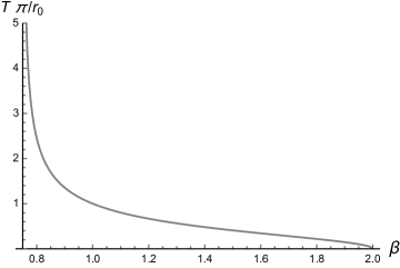
Figure 1: Temperature of the deformed black brane, as a function of $\beta$.

The deformed black brane temperature diverges at $\beta\to 3/4$, having imaginary values for either $\beta<3/4$ or $\beta>2$. As the deformed black brane temperature cannot attain divergent values or imaginary ones, the analysis of the deformed black brane temperature constrains the $\beta$ parameter in the open range $\beta\in(3/4,2)$. One can invert Eq. (39) to express $r_{0}$ as

$$r_{0}=\pi\sqrt{\frac{3-4\beta}{\beta-2}}T\ .$$ (40)

Finally, the free energy can be read off, when Eq. (40) is replaced into (37), yielding

$$\!\!\!\!\!\!\!F=\frac{\pi^{3}V}{8G}\left(\frac{11-15\beta+3\beta^{2}}{2}\right)\left(\frac{3-4\beta}{\beta-2}\right)^{2}T^{4}\ .$$ (41)

The state functions can now be computed using standard statistical mechanics in the canonical ensemble

$$\!\!\!\!\!\!\!\!\!\!\!\!\!\!s = -\frac{1}{V}\frac{\partial F}{\partial T}\!=\!-\frac{\pi^{3}}{2G}\!\left(\frac{11\!-\!15\beta\!+\!3\beta^{2}}{2}\right)\!\!\left(\frac{3-4\beta}{\beta-2}\right)^{\!\!2}\!T^{3},$$ (42)

$$\!\!\!\!\!\!\!\!P \!=\! \!-\frac{\partial F}{\partial V}\!=\!-\frac{\pi^{3}}{8G}\!\left(\frac{11\!-\!15\beta\!+\!3\beta^{2}}{2}\right)\left(\frac{3\!-\!4\beta}{\beta-2}\right)^{2}\!T^{4}\ ,$$ (43)

$$\!\!\!\!\!\!\varepsilon \!=\! \frac{F}{V}\!-\!Ts\!=\!\frac{5\pi^{3}}{8G}\!\left(\frac{11\!-\!15\beta\!+\!3\beta^{2}}{2}\right)\!\left(\frac{3-4\beta}{\beta-2}\right)^{2}\!T^{4}.$$ (44)

Despite the negative sign in front of entropy and pressure, these quantities are positive in the range of $\beta$ to be considered in the analysis to come in the next session. For a perfect fluid, the energy-momentum tensor reads

$$T^{ab}=\left(\varepsilon+P\right)u^{a}u^{b}+Pg^{ab}.$$ (45)

From Eqs. (43, 44), evaluated at the boundary, the trace of the energy-momentum tensor (45) is given by

$$\!\!\!\!\!\!\!\!\!g_{\mu\nu}T^{\mu\nu} \!=\! -\varepsilon+3P$$ (46)

$$= -\frac{\pi^{3}}{G}\left(\frac{11-15\beta+3\beta^{2}}{2}\right)\!\left(\frac{3-4\beta}{\beta-2}\right)^{\!\!2}T^{4}.$$

For future reference, changing $T$ to $r_{0}$ using (40), the entropy density in Eq. (42) can be written as,

$$s=-\frac{r_{0}^{3}}{2G}\left(\frac{11-15\beta+3\beta^{2}}{2}\right)\left(\frac{3-4\beta}{\beta-2}\right)^{1/2}\,.$$ (47)

As the entropy of a black hole obtained from Einstein’s equations is proportional to its area, in the particular case of metric (23) we have a deformation of a Schwarzschild black hole that is asymptotically AdS. This deformation breaks the spherical symmetry of our problem, and we have just used the AdS/CFT correspondence to compute the surface area of the black hole, i.e. $A=4GsV$.

IV $\frac{\eta}{s}$ for the AdS₅–Schwarzschild deformed black brane

As metric (23) arises from a deformation of the AdS₅–Schwarzschild mgd1 , the same action-dependent results may be applied. The metric determinant, $g$, is such that $\sqrt{-g}=\frac{r_{0}^{4}}{u^{5}}\sqrt{\frac{N}{A}}$, where, from now on, $N$ and $A$ refer respectively to $N(u)$ and $A(u)$.

Consider a bulk perturbation $h_{xy}$ such that:

$$ds^{2}=ds^{2}_{{\rm AdS}_{5}-{SD}}+2h_{xy}\mathrm{d}x\mathrm{d}y\ ,$$ (48)

where $ds^{2}_{{\rm AdS}_{5}-{SD}}$ denotes the AdS₅–Schwarzschild deformed black brane metric, Eq. (23). In appendix B we show that the field associated to the perturbation propagates with the speed of light, this signals that no anomaly is present when it comes to the spacetime causal structure.

Recall Eq. (5), for $h_{xy}^{(0)}$ being the perturbation added to the boundary theory, which is asymptotically related to $h_{xy}$, the bulk perturbation, by

$$g^{xx}h_{xy}\sim h_{xy}^{(0)}\left(1+h_{xy}^{(1)}u^{4}\right)\ ,$$ (49)

according to Eq. (12). Notice that one can directly use the results for a massless scalar field, as $g^{xx}h_{xy}$ obeys the EOM for a massless scalar field Son:2009zzc ; son_hydro . Besides, the deformed AdS₅–Schwarzschild black brane has the same asymptotic behavior of the AdS₅–Schwarzschild black brane (namely, Eq. (10)). One can identify $g^{xx}h_{xy}$ as the bulk field, $\upvarphi$, which plays the role of an external source of a boundary operator, in this case $\tau^{xy}$. Therefore, one can directly obtain the response $\updelta\left\langle\tau^{xy}\right\rangle$, from Eq. (13),

$$\updelta\left\langle\tau^{xy}\right\rangle=\frac{r_{0}^{4}}{16\pi G}4h_{xy}^{(1)}h_{xy}^{(0)}\ ,$$ (50)

where it is now convenient to reintroduce the $1/16\pi G$ factor. Comparing Eqs. (5) and (50) yields

$$i\omega\eta=\frac{r_{0}^{4}}{4\pi G}h_{xy}^{(1)}.$$ (51)

Taking the ratio between Eq. (51) and the entropy (47) we find

$$\!\!\!\!\!\!\!\!\!\!\!\!\!\!\frac{\eta}{s}=-\frac{r_{0}}{\pi}\left[\left(\frac{1}{11-15\beta+3\beta^{2}}\right)\left(\frac{\beta-2}{3-4\beta}\right)^{1/2}\right]\frac{h_{xy}^{\left(1\right)}}{i\omega},$$ (52)

​​where $h_{xy}^{(1)}$ is the solution of the EOM for the perturbation $g^{xx}h_{xy}\equiv\upvarphi$, which is that of a massless scalar field Son:2009zzc ; son_hydro

$$\nabla_{M}\left(\sqrt{-g}g^{MN}\nabla_{N}\upvarphi\right)=0\ .$$ (53)

Considering a stationary perturbation, given by the form $\upvarphi(u,t)=\upphi(u)e^{-i\omega t}$, the perturbation equation reduces to a second-order ODE for $\upphi(u)$,

$$\ddot{\upphi}+\frac{1}{2}\left(\frac{\dot{N}A}{2N}+\frac{N\dot{A}}{A}-\frac{3}{u}\right)\dot{\upphi}+\frac{1}{NA}\frac{\omega^{2}}{r_{0}^{2}}\upphi=0\ .$$ (54)

To derive the solution of Eq. (54), two boundary conditions are imposed: the incoming wave boundary condition in the near-horizon region, corresponding to $u\rightarrow 1$, and a Dirichlet boundary condition at the AdS boundary, $\upphi(u\rightarrow 0)=\upphi^{(0)}$, where $h_{xy}^{(0)}=\upphi^{(0)}e^{-i\omega t}$.

The incoming wave boundary condition near the horizon is obtained by solving Eq. (54) in the limit $u\rightarrow 1$. After a straightforward computation one finds the following

$$\upphi\propto\exp\left(\pm i\frac{\omega}{r_{0}}\sqrt{\frac{4\beta-3}{\beta-1}}\sqrt{1-u}\right).$$ (55)

This solution has a natural interpretation using tortoise coordinates, allowing one to identify it as a plane wave natsuume . The positive exponent represents an outgoing wave, whereas the negative one describes the wave incoming to the horizon, which, according to the near-horizon boundary condition, allows us to fix

$$\upphi\approx\exp\left(-i\frac{\omega}{r_{0}}\sqrt{\frac{4\beta-3}{\beta-1}}\sqrt{1-u}\right).$$ (56)

Next we solve Eq. (54) for all $u\in[0,1]$ as a power series in $\omega$. As we are interested in the hydrodynamic limit of this solution, i.e. $\omega\rightarrow 0$, it is sufficient to keep the series up to linear order:

$$\upphi(u)=\Phi_{0}(u)+\omega\Phi_{1}(u)\ .$$ (57)

Since the second term in Eq. (54) is of order $\omega^{2}$, it can be neglected. By direct integration the solution reads

$$\Phi_{i}=C_{i}+K_{i}\int\frac{u^{3}}{\sqrt{N(u)A(u)}}\,\mathrm{d}u\ ,$$ (58)

for $C_{i}$ and $K_{i}$ the integration constants and $i=0,1$. Thus, according to Eq. (57), we have

$$\upphi=\left(C_{0}+\omega C_{1}\right)+\left(K_{0}+\omega K_{1}\right)\int\frac{u^{3}}{\sqrt{N(u)A(u)}}\,\mathrm{d}u\ .$$ (59)

In order to impose the boundary conditions we expand the integral (59) around $u\rightarrow 0$ and $u\rightarrow 1$. It yields, up to leading order in the respective expansions,

$$\!\!\!\!\!\!\!\!\!\!\!\!\!\!\int\!\frac{u^{3}}{\sqrt{NA}}\,\mathrm{d}u\! = \!\begin{cases}\frac{u^{4}}{4}\ ,&\;\;\;\text{for}\;\;u\rightarrow 0,\\ \frac{3-4\beta}{\beta-1}\sqrt{\frac{\beta-1}{3-4\beta}}\sqrt{1-u}\ ,&\;\;\;\text{for}\;\;u\rightarrow 1.\end{cases}$$ (60)

The first pair of integration constants is fixed by the Dirichlet boundary condition

$$\!\!\!\!\!\!\!\!\!\!\!\!\!\!\lim_{u\rightarrow 0}\upphi=\left(C_{0}+\omega C_{1}\right)+\left(K_{0}+\omega K_{1}\right)\lim_{u\rightarrow 0}\frac{u^{4}}{4}=\upphi^{(0)},$$ (61)

implying that $\left(C_{0}+\omega C_{1}\right)=\upphi^{(0)}$. Near the horizon one has

$$\upphi\approx\upphi^{(0)}-\left(K_{0}+\omega K_{1}\right)\frac{(4\beta-3)}{\beta-1}\sqrt{\frac{\beta-1}{4\beta-3}}\sqrt{1-u}.$$ (62)

Expanding Eq. (56) up to $\mathcal{O}(\omega)$ yields

$$\upphi\propto 1-i\frac{\omega}{r_{0}}\sqrt{\frac{4\beta-3}{\beta-1}}\sqrt{1-u}.$$ (63)

It is straightforward to see that Eq. (62) fixes the proportionality according to

$$\upphi\approx\upphi^{(0)}-i\upphi^{(0)}\frac{\omega}{r_{0}}\sqrt{\frac{4\beta-3}{\beta-1}}\sqrt{1-u}.$$ (64)

Comparison between Eqs.(62) and (64) immediately fixes the second pair of integration constants:

$$\left(K_{0}+\omega K_{1}\right)=i\upphi^{(0)}\frac{\omega}{r_{0}}\left(\frac{\beta-1}{4\beta-3}\right)\frac{|4\beta-3|}{|\beta-1|}.$$ (65)

Then the full solution reads

$$\!\!\!\upphi\!=\!\upphi^{(0)}\left(1\!+\!i\frac{\omega}{r_{0}}\left(\frac{\beta\!-\!1}{4\beta\!-\!3}\right)\frac{|4\beta\!-\!3|}{|\beta\!-\!1|}\int\!\frac{u^{3}}{\sqrt{NA}}\,\mathrm{d}u\right)\ .$$ (66)

Accordingly, the full time-dependent perturbation

$$\upvarphi=g^{xx}h_{xy}=\upphi(u)e^{-i\omega t}\ ,$$ (67)

is asymptotically given by:

$$g^{xx}h_{xy}\sim e^{-i\omega t}\upphi^{(0)}\left(1+i\frac{\omega}{r_{0}}\left(\frac{\beta-1}{4\beta-3}\right)\frac{|4\beta-3|}{|\beta-1|}\frac{u^{4}}{4}\right)\ .$$ (68)

Eqs. (49, 68) yield

$$h_{xy}^{(1)}=\frac{i\omega}{4r_{0}}\left(\frac{\beta-1}{4\beta-3}\right)\frac{|4\beta-3|}{|\beta-1|}\ ,$$ (69)

where $h_{xy}^{(0)}=\upphi^{(0)}e^{-i\omega t}$. The term multiplying $\frac{i\omega}{4r_{0}}$ in Eq. (69) can be visualized in the following plot:

Figure 2: $4r_{0}\frac{h_{xy}^{(1)}}{i\omega}$ as a function of $\beta$.

Therefore we have different signs depending on the value of $\beta$,

$$\begin{cases}h_{xy}^{(1)}=-\frac{i\omega}{4r_{0}}&\frac{3}{4}<\beta<1\ ,\\ h_{xy}^{(1)}=\frac{i\omega}{4r_{0}}&\beta<\frac{3}{4}\text{ or }\beta>1\ .\end{cases}$$ (70)

A negative value for $h_{xy}^{(1)}$, without further constraints, would imply a negative value of $\frac{\eta}{s}$, i.e., a negative viscosity or entropy density, which would violate the second law of thermodynamics. Therefore, demanding thermodynamical consistency leads to the following first bound in the deformation parameter: either $\beta<\frac{3}{4}\ \text{or}\ \beta>1$.

Now, substituting (69) in Eq. (52) yields

$$\frac{\eta}{s}=\begin{cases}-\frac{1}{4\pi}\left(\frac{1}{11-15\beta+3\beta^{2}}\right)\left(\frac{\beta-2}{3-4\beta}\right)^{1/2}\!\!,&\beta>1\\ \frac{1}{4\pi}\left(\frac{1}{11-15\beta+3\beta^{2}}\right)\left(\frac{\beta-2}{3-4\beta}\right)^{1/2}\!\!,&\beta<1\end{cases}\ .$$ (71)

Fig. 3 illustrates Eq. (71) as a function of $\beta$.

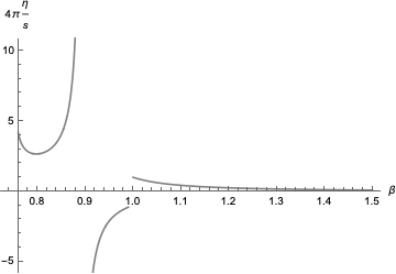
Figure 3: $\frac{\eta}{s}$ ratio of the deformed black brane, as a function of $\beta$.

For the precise value $\beta=1$, the deformed black brane $\frac{\eta}{s}$ ratio is exactly $\frac{1}{4\pi}$, recovering the KSS result for the AdS₅–Schwarzschild black brane. Besides, Fig. 3 shows the divergence of $\frac{\eta}{s}$ for $\beta\approxeq 0.9$ as well as the vanishing of the $\frac{\eta}{s}$ ratio, for $\beta=2$.

Therefore, a priori the deformation parameter can attain the ranges

$$0.75<\beta<0.9\;\;\;\text{and}\quad 1<\beta\leq 2.$$ (72)

The value $\beta\leq 2$ is seen from (71), since $\beta=2$ makes that quantity equal to zero, whereas the range $0.9\leq\beta<1$ imply $\frac{\eta}{s}<0$, which has no physical significance. The saturation $\frac{\eta}{s}=\frac{1}{4\pi}$, corresponding to to the infinite ’t Hooft coupling limit Cremonini:2011iq , then implies $\beta=1$. This result has been expected, as this case recovers the AdS₅–Schwarzschild black brane (9). However, an additional consistence test must take into account Eq. (24), that defines the deformed AdS₅–Schwarzschild black brane event horizon. In fact, let us call by $u_{\beta}=1/r_{\beta}$ the solution of the algebraic equation $N(u)=0$, in (24). The first consistence test must regard the choice of $\beta$ in such a way that it produces a real event horizon. Therefore, this restricts more the possible range for $\beta$, from $1<\beta\leq 2$ to $1<\beta\leq 1.384$. A second consistence test involves the fact that the $r_{0}=\lim_{\beta\to 1}r_{\beta}$ horizon, corresponding to the standard AdS₅–Schwarzschild black brane event horizon, is of Killing type. Along our previous calculations, the horizon is assumed to be at $r_{0}$. For it to be a good approximation in the proposed ranges of $\beta$, in such a way that $\left|r_{0}-r_{\beta}\right|\lesssim 10^{-2}$, we must restrict a little more the allowed range to $1<\beta\lesssim 1.2$, since for the another range $0.75<\beta<0.9$ the condition $\left|r_{0}-r_{\beta}\right|\lesssim 10^{-2}$ already holds. Hence, the $\beta$ parameter is restricted into the ranges

$$0.75<\beta<0.9\;\;\;\text{and}\quad 1<\beta\lesssim 1.2.$$ (73)

To end this section we present a comparison between results obtained with metric (23) and the conventional AdS${}_{5}-$Schwarzschild, which also gives us insight on the effect of the parameter $\beta$. Denoting $T_{S}$, $s_{S}$ and $\left(\frac{\eta}{s}\right)_{S}$ the temperature, entropy density and shear viscosity to entropy density of the standard AdS${}_{5}-$Schwarzschild spacetime, respectively, one can check that the corresponding positive quantities for fixed $\beta=1.05$ are

$$\begin{aligned} {\color[rgb]{0,0,0}\!\!\!\!\!T=0.89T_{S},\qquad s=1.82s_{S},\qquad\frac{\eta}{s}=0.54\left(\frac{\eta}{s}\right)_{S}},\end{aligned}$$ (74)

For instance, if $\beta=1.2$ one finds

$$\begin{aligned} \!T=0.67T_{S},\qquad s=6.03s_{S},\qquad\frac{\eta}{s}=0.17\left(\frac{\eta}{s}\right)_{S}\ .\end{aligned}$$ (75)

Considering the results (74) and (75), the effects of the deformation in the metric are clear, changing thermodynamics and hydrodynamics by a numerical factor. In the range $1<\beta\leq 1.2$, there is a violation of the KSS bound. One can speculate that the violation comes from the fact that the solution under investigation does not obey Einstein’s equations of GR, since it was obtained via an embedding in a higher dimensional space-time, whose evolution is governed by an equation that has the Einstein’s field equations as a certain limit, c.f. Eq. (19). Fig. 3 illustrates that the range $0.75<\beta<0.9$ is formally allowed, wherein the deformation parameter makes the KSS bound not to be violated. The existence of a range where the KSS bound is violated, namely $1<\beta\lesssim 1.2$, but no pathologies in causality of space-time or thermodynamic functions can be seen, is also one of the main results of this work. The meaning of the $\beta$ parameter will be further discussed in Sec. V. We emphasize that it is a free constant parameter, generating a family of deformed AdS₅–Schwarzschild black branes, which has been constrained for different reasons. We have imposed compliance with the second law of thermodynamics, thus discarding the ranges which would yield negative values of $\frac{\eta}{s}$. Therefore, the family of solutions obtained with the allowed values of $\beta$ can be an interesting result worthy further investigation, mainly in the AdS/QCD correspondence. The embedding bulk scenario and ADM procedure, in which the deformed AdS₅–Schwarzschild black brane was obtained, provides one more counterexample setup to the KSS bound conjecture. Besides, these results can play a relevant role on the QGP, whose measured viscosity is close to the KSS bound, possibly violates the bound Cherman:2007fj . In the next section we also address a possible scenario that corroborates to the violation of the KSS bound in the range $1<\beta\lesssim 1.2$.

V Scrutinizing the $\beta$ parameter

This section is devoted to clarify aspects of the $\beta$ parameter. If one considers AdS/CFT in the braneworld, it relates the electric part of the Weyl tensor $\mathcal{E}_{\mu\nu}$ in Eq. (17), that represents (classical) gravitational waves in the bulk, to the expectation value $\langle T_{\mu\nu}\rangle$ of the (renormalized) energy-momentum tensor of conformal fields on the brane Shiromizu:2001jm ; Kanno:2002iaa . Besides, the presence of the brane introduces a normalizable 4D graviton and an ultraviolet (UV) cut-off in the CFT, proportional to $\sigma^{-1}$. The general-relativistic limit requires $\sigma\to\infty$, corresponding to a geometric rigid brane with infinite tension. In the AdS/CFT setup, $\mathcal{E}^{\nu}_{\;\mu}\sim\ell_{p}^{2}\langle T_{\;\mu}^{\nu}\rangle$. Since the electric part of the Weyl tensor is traceless, such a correspondence would imply that $\langle T_{\;\mu}^{\mu}\rangle\equiv\langle T\rangle=0$. In other words, it would hold in the case where the conformal symmetry is not anomalous. Eq. (46) therefore indicates a conformal anomaly due to the quantum corrections induced by $\beta$. Eq. (46) yields $\langle T\rangle\neq 0$ for any value of $\beta$ but $\beta=1$. It is in full compliance with the fact that if $\langle T\rangle=0$, then the UV cut-off would be required to be much shorter than any physical length scale involved. Besides, $\langle T\rangle=0$ for any value of $\beta$ would also demand the absence of any intrinsic 4D length associated with the background, otherwise the CFT is affected by that scale. For the deformed AdS₅–Schwarzschild black brane, the horizon radius $r_{0}$ is a natural length scale and one therefore expects that only CFT modes with wavelengths much shorter than $r_{0}$, that are much larger than $\sigma^{-1}$, can propagate freely. Bulk perturbations at the boundary work as sources the CFT fields, and can produce $\langle T\rangle=0$.

Of course, this requires that the UV cut-off be much shorter than any physical length scale in the system. For a black hole, the horizon radius is a natural length scale and one therefore expects that only CFT modes with wavelengths much shorter than $r_{\rm h}$, that are still much larger than $\sigma^{-1}$, propagate freely Casadio:2003jc .

Besides, for the deformed AdS₅–Schwarzschild black brane, one can emulate the holographic computation of the Weyl anomaly Henningson:1998gx . In fact, denoting $a$ and $c$ central charges of the conformal gauge theory, according to Eq. (24) of Ref. Cremonini:2011iq ,

$$\!\!\!\!\!\!\!\!\langle T^{\mu}_{\;\,\mu}\rangle_{\rm CFT} = \frac{c}{16\pi^{2}}\left(R_{\mu\nu\rho\sigma}R^{\mu\nu\rho\sigma}-2R_{\mu\nu}R^{\mu\nu}+\frac{1}{3}R^{2}\right)$$ (76)

$$-\frac{a}{16\pi^{2}}\left(R_{\mu\nu\rho\sigma}R^{\mu\nu\rho\sigma}\!-\!4R_{\mu\nu}R^{\mu\nu}\!+\!R^{2}\right),$$

where the terms in parentheses are, respectively, the Euler density and the square of the Weyl curvature.

It is worth to mention the splitting of the allowed range of $\beta$ into $0.75<\beta<0.9$ and $1<\beta\lesssim 1.2$. Firstly, considering the range $1<\beta\lesssim 1.2$, Ref. Kats:2007mq studied an effective 5D bulk gravity dual, and showed that the KSS bound is violated, whenever the central charges in the Weyl anomaly (76) satisfy $|c-a|/c\ll 1$. In this way, the inequality $c>a$ yields the KSS bound to be violated Buchel:2008vz ; viol1 . Ref. Kats:2007mq showed that, as an effect of curvature squared corrections in the AdS bulk, the shear viscosity-to-entropy density ratio can be expressed as $\frac{\eta}{s}=\frac{1}{4\pi}\frac{a}{c}+\mathcal{O}(1/N^{2})$. Therefore, in the large $N$ limit, the equality $\frac{\eta}{s}\approxeq\frac{1}{4\pi}\frac{a}{c}$ holds, and the central charges ratio drive the KSS bound violation, whenever $c\neq a$. In fact, the well-known $\mathcal{N}=4$, SU($N$) super-Yang–Mills theory implies $a=c$, however nothing precludes that $c\neq a$ in other cases Kats:2007mq .

Secondly, now considering the allowed range $0.75<\beta<0.9$, the deformed AdS₅–Schwarzschild black brane, on the boundary $u\to 0$, the square of the Weyl curvature can be expanded as

$$\!\!\!\!\!\!\!N^{2}\left(\frac{40}{3}+\frac{32}{3}(\beta-1)u^{4}+8(\beta-1)u^{6}\right)+\mathcal{O}\left(u^{7}\right),$$ (77)

and the Euler density as

$$\!\!\!\!\!\!\!N^{2}\left(120+96(\beta-1)u^{4}+72(\beta-1)u^{6}\right)+\mathcal{O}\left(u^{7}\right),$$ (78)

where $N^{2}=\pi L^{3}/2G$. One notices in Eqs. (77, 78) that the leading-order terms contain factors $(\beta-1)u^{p}$, for $p=4,6$. Therefore, the limits $\beta\to 1$, corresponding to the standard AdS₅–Schwarzschild black brane, and the boundary $u\to 0$ limit, are indistinguishable. Hence, the limit $u\to 0$ yields

$$\langle T^{\mu}_{\;\,\mu}\rangle_{\rm CFT}=\frac{520N^{2}}{9},$$ (79)

having the same result of the standard AdS₅–Schwarzschild black brane.

It is worth to compare an already known result about $\frac{\eta}{s}$ in presence of quantum corrections. In fact, Ref. Myers:2008yi discusses quantum corrections to the $\frac{\eta}{s}$ ratio, by including higher derivative terms with the 5-form RR flux to the calculation. Corrections are implemented as inverse powers of the colour number $N$, and the leading $1/N^{2}$ correction adds two corrections terms to entropy density, $s$, modifying $\frac{\eta}{s}$ in QCD strongly coupled QGP. Its original value, $\frac{1}{4\pi}$, is increased by approximately 37%, roughly 22% due to the first correction term and 15% due to the second. As discussed in this section, our setup yields corrections that can be interpreted as quantum ones, induced by $\beta$, as expressed in Eq. (46). For $\beta=0.75$, consisting of a lower bound for $\beta$, the $\frac{\eta}{s}$ ratio increases $\sim 4.1$ times the original $\frac{\eta}{s}=\frac{1}{4\pi}$ value. In the range $0.75<\beta<0.9$, there is a minimum at $\beta\approx 0.8$, for which the shear viscosity-to-entropy ratio equals $2.5$ the KSS bound. In the range $1<\beta\leq 1.2$, we showed that the KSS bound is violated. For example, as analyzed in Eq. (74, 75), the value $\beta=1.05$ yields $\frac{\eta}{s}=0.54\left(\frac{\eta}{s}\right)_{S}$, whereas taking $\beta=1.2$ implies that $\frac{\eta}{s}=0.17\left(\frac{\eta}{s}\right)_{S}$.

VI Concluding remarks and perspectives

The ADM procedure was used to derive a family of AdS₅–Schwarzschild deformed gravitational backgrounds, involving a free parameter, $\beta$, in the black brane metric (23, 24, 25). Computing the $\frac{\eta}{s}$ ratio for this family provided two possible values to $\beta$. The first one, $\beta=1$, was physically expected, corresponding to the AdS₅–Schwarzschild black brane. Besides the importance of the result itself, in particular for the membrane paradigm of AdS/CFT, it has a good potential for relevant applications, mainly in AdS/QCD. Taking into account the thermodynamics that underlies the family of deformed black branes solutions, arising from the Einstein–Hilbert action in the bulk, with a Gibbons–Hawking term and a counter-term that eliminates divergences, yields the deformed black brane temperature (39). This expression, together with the fact that the event horizon of the deformed AdS₅–Schwarzschild black brane must assume real values, constrain the range of the free parameter $\beta$ in the range (73).

Although we have derived our results using the ADM formalism, in a bulk embedding scenario, the KSS bound violation in the range $1<\beta\leq 2$ represents, as a matter of speculation, a possible smoking gun towards the fact that the deformed AdS₅–Schwarzschild black brane (23), with metric coefficients (24, 25), might be, alternatively, derived from an action with higher curvature terms. However, up to our knowledge, no result has been obtained in this aspect, yet.

The family of AdS₅–Schwarzschild deformed black branes, here derived using the ADM formalism, is also not the first example in the literature of a setup that violates the KSS bound and does not involve higher derivative theories of gravity, in the gauge/gravity correspondence. In fact, strongly coupled $\mathcal{N}=4$ super-Yang–Mills plasmas can describe pre-equilibrium stages of the quark-gluon plasma (QGP) in heavy-ion collisions. In this setup, the shear viscosity, transverse to the direction of anisotropy, was shown to saturate the KSS viscosity bound Rebhan:2011vd . Besides, anisotropy in the shear viscosity induced by external magnetic fields in a strongly coupled plasma also provided violation in the KSS bound Critelli:2014kra . Theories with higher order curvature terms in the action, in general, comprise attempts of describing quantum gravity. Hence, one is restricted to consider CFT for which the central charges satisfy $|c-a|/c\ll 1$ and $c>a$, in such a way that still $c\sim a\gg 1$, also yielding violation of the KSS bound Buchel:2008vz ; viol1 . Up to now, the equations of motion for 5D actions with higher curvature terms up to third order are already established in the literature, but it has been not possible to obtain the deformed AdS₅–Schwarzschild black brane (23) yet as an exact solution to any of them. We keep trying to compute higher curvature terms, including fourth order terms, and we have not exhausted all the possibilities, yet. Any effective action is expected to contain curvature terms of higher order, each one of them accompanying their respective coefficients. To derive a sensible derivative expansion, one should restrict to the classes of CFTs wherein these coefficients are proportional to inverse powers of the central charge $c$ Buchel:2008vz .

As large-$N_{c}$ gauge theories considered by AdS/CFT are good approximations to QCD, one could expect that the result of Eq. (15) may be applied to the QGP, which is a natural phenomenon in QCD, when at high enough temperature the quarks and gluons are deconfined from protons and neutrons to form the QGP qgpexp2 . In fact, experiments in the RHIC have shown that the QGP behaves like a viscous fluid with very small viscosity, which implies that the QGP is strongly-coupled, thus discarding the possibility of using perturbative QCD to the study of the plasma. Therefore, the new AdS₅–Schwarzschild deformed black brane (23) can be widely used to probe additional properties in the AdS/QCD approach. As in the holographic soft-wall AdS/QCD the AdS₅-Schwarzschild black brane provides a reasonable description of mesons at finite temperature BoschiFilho:2004ci , we can test if using the AdS₅–Schwarzschild deformed black brane derives a more reliable meson mass spectra for the mesonic states and their resonances, better matching experimental results. Besides, the new AdS₅–Schwarzschild deformed black brane can be also explored in the context of the Hawking–Page transition and information entropy Bernardini:2016hvx ; Braga:2016wzx .

Appendix A

$$f(r,r_{0},\beta) = -\frac{1}{r^{10}}\Bigg{\{}-\left(10(\beta-1)+r^{6}-3r^{2}r_{0}^{4}\right)\left(\beta+r^{6}-r^{2}r_{0}^{4}-1\right)+\frac{4r^{8}\left(-2\beta+r^{6}+r^{2}r_{0}^{4}+2\right)^{2}}{\left(\beta+r^{6}-r^{2}r_{0}^{4}-1\right)^{2}}$$ (80)

$$+\frac{4r^{8}\left(4r^{12}\!+\!8(2\!-\!3\beta)r^{8}r_{0}^{4}\!+\!(20\beta\!-\!23)r^{4}r_{0}^{8}\!+\!3(4\beta\!-\!1)r_{0}^{12}\right)^{2}}{\left(2r^{8}-5r^{4}r_{0}^{4}+3r_{0}^{8}\right)^{2}\left(2r^{4}+(1-4\beta)r_{0}^{4}\right)^{2}}$$

$$-\frac{2r^{8}\left(8r^{16}-60r^{12}r_{0}^{4}+6(40\beta(2\beta-3)+67)r^{8}r_{0}^{8}+(4\beta-1)(20\beta+43)r^{4}r_{0}^{12}-9(1-4\beta)^{2}r_{0}^{16}\right)}{\left(2r^{8}-5r^{4}r_{0}^{4}+3r_{0}^{8}\right)\left(2r^{4}+(1-4\beta)r_{0}^{4}\right)^{2}}$$

$$+\frac{1}{2r^{4}\!+\!(1\!-\!4\beta)r_{0}^{4}}[r^{2}\left(2r^{8}\!+\!2r^{6}\!-\!5r^{4}r_{0}^{4}\!+\!(1\!-\!4\beta)r^{2}r_{0}^{4}\!+\!3r_{0}^{8}\right)\left(\beta\!+\!r^{6}\!-\!r^{4}\!-\!r^{2}r_{0}^{4}\!-\!1\right)]$$

$$+\!\frac{4r^{8}\left(r^{6}\!+\!r^{2}r_{0}^{4}\!+\!2\!-\!2\beta\right)\left(4r^{12}\!+\!8(2\!-\!3\beta)r^{8}r_{0}^{4}\!+\!3(4\beta\!-\!1)r_{0}^{12}\right)}{\left(2r^{4}\!-\!3r_{0}^{4}\right)\left(r^{4}\!-\!r_{0}^{4}\right)\left(2r^{4}\!+\!(1\!-\!4\beta)r_{0}^{4}\right)\left(\beta\!+\!r^{6}\!-\!r^{2}r_{0}^{4}\!-\!1\right)}$$

$$+2r^{8}\left(\frac{2r^{8}+5r^{4}r_{0}^{4}-9r_{0}^{8}}{2r^{8}-5r^{4}r_{0}^{4}+3r_{0}^{8}}-\frac{4r^{4}}{2r^{4}+(1-4\beta)r_{0}^{4}}+\frac{r^{2}\left(3r^{4}-r_{0}^{4}\right)}{\beta+r^{6}-r^{2}r_{0}^{4}-1}\right)\Bigg{\}}$$

Appendix B

We will show that the graviton propagates at the speed of light. Throughout this appendix we make $r_{0}=1$, and the metric (23) is written in coordinates $\{t,r,x,y,z\}$, where $r=u^{-1}$ according to the present convention.

Consider a perturbation of the form (48). As discussed in the text, the perturbation $h_{xy}$ can be considered as a field on its own, hence we define $\varphi=g^{xx}h_{xy}$. We now identify the action as $S\sim S_{0}+S_{2}$, where $S_{0}$ does not have any contribution from $\varphi$, i.e. it is the action as studied in Sect. III.1, whereas $S_{2}$ contains contributions of $\varphi$ and its derivatives. Let

$$\varphi=\int dk\Phi(r)e^{-i\omega t+ikr+iqz}\ ,$$ (81)

where $dk=\frac{d\omega dqdk}{\left(2\pi\right)^{3}}$, so that $S_{2}\propto\int\mathcal{L}(\Phi,\Phi^{\prime},\Phi^{\prime\prime})$, the proportionality factor is discarded. The Lagrangian reads

$$\begin{aligned} \sqrt{\frac{A}{N}}\mathcal{L}&=\Phi^{2}\left[-6r^{5}+2rA+r^{2}\left(ikA+2A^{\prime}+\frac{2AN^{\prime}}{N}\right)+\frac{7}{2}r^{3}\left(-q^{2}-Ak^{2}+\frac{\omega^{2}}{N}\right)+r^{3}\left(ikA^{\prime}+ikA\frac{N^{\prime}}{N}+\frac{AN^{\prime\prime}}{2N}\right.\right.\\ &\left.\left.+\frac{A^{\prime}N^{\prime}}{4N}-\frac{AN^{\prime 2}}{4N^{2}}\right)\right]+\Phi\Phi^{\prime}\left[r^{2}\left(8+7ikr\right)A+A^{\prime}+\frac{AN^{\prime}}{N}\right]+\frac{3}{2}\Phi^{\prime 2}A+2A\Phi\Phi^{\prime\prime}\ .\end{aligned}$$ (82)

For an action dependent on a single field up to its second derivative one can show immediately that

$$\delta S=\delta S_{bdy}+\int dr\delta\Phi\left[\left(\frac{\partial\mathcal{L}}{\partial\Phi^{\prime\prime}}\right)^{\prime\prime}-\left(\frac{\partial\mathcal{L}}{\partial\Phi^{\prime}}\right)^{\prime}+\frac{\partial\mathcal{L}}{\partial\Phi}\right]\ ,$$ (83)

$\delta S_{bdy}$ are surface terms, while the factor inside the integral is the equation of motion.

The momentum vector is $k^{\mu}=(\omega,k,0,0,q)$. Evaluating the EOM from (83) using Lagrangian (82) we obtain, in the limit $k^{\mu}\mapsto\infty$, the following

$$k_{\mu}k^{\mu}=0\ ,$$ (84)

i.e. the EOM for a light-ray. This shows that the graviton – field associated to the perturbation (48) – propagates with the speed of light.

References

- (1) Rangamani M 2009 Class. Quant. Grav. 26 224003 (Preprint eprint 0905.4352)
- (2) Bhattacharyya S, Hubeny V E, Minwalla S and Rangamani M 2008 JHEP 02 045 (Preprint eprint 0712.2456)
- (3) Hubeny V E, Minwalla S and Rangamani M 2012 The fluid/gravity correspondence Black holes in higher dimensions pp 348–383 [,817(2011)] (Preprint eprint 1107.5780)
- (4) Casadio R, Ovalle J and da Rocha R 2015 Class. Quant. Grav. 32 215020 (Preprint eprint 1503.02873)
- (5) da Rocha R 2017 Phys. Rev. D95 124017 (Preprint eprint 1701.00761)
- (6) Casadio R and da Rocha R 2016 Phys. Lett. B763 434–438 (Preprint eprint 1610.01572)
- (7) Fernandes-Silva A, Ferreira-Martins A J and da Rocha R 2019 Phys. Lett. B791 323–330 (Preprint eprint 1901.07492)
- (8) Iqbal N and Liu H 2009 Phys. Rev. D79 025023 (Preprint eprint 0809.3808)
- (9) Fernandes-Silva A, Ferreira-Martins A J and da Rocha R 2018 Eur. Phys. J. C 78 631 (Preprint eprint 1803.03336)
- (10) Casadio R, Fabbri A and Mazzacurati L 2002 Phys. Rev. D65 084040 (Preprint eprint gr-qc/0111072)
- (11) Casadio R, Cavalcanti R T and da Rocha R 2016 Eur. Phys. J. C76 556 (Preprint eprint 1601.03222)
- (12) Maartens R and Koyama K 2010 Living Rev. Rel. 13 5 (Preprint eprint 1004.3962)
- (13) Eling C and Oz Y 2010 JHEP 02 069 (Preprint eprint 0906.4999)
- (14) Antoniadis I 1990 Phys. Lett. B246 377–384
- (15) Antoniadis I, Arkani-Hamed N, Dimopoulos S and Dvali G R 1998 Phys. Lett. B436 257 (Preprint eprint hep-ph/9804398)
- (16) Yagi K, Hatsuda T and Miake Y 2005 Camb. Monogr. Part. Phys. Nucl. Phys. Cosmol. 23 1–446
- (17) Song H 2013 Nucl. Phys. A904-905 114c–121c (Preprint eprint 1210.5778)
- (18) Adare A et al. (PHENIX) 2007 Phys. Rev. Lett. 98 172301 (Preprint eprint nucl-ex/0611018)
- (19) Song H and Heinz U W 2008 Phys. Lett. B658 279–283 (Preprint eprint 0709.0742)
- (20) Ferreira-Martins A J, Meert P and da Rocha R 2019 Eur. Phys. J. C79 646 (Preprint eprint 1904.01093)
- (21) Casadio R, Fabbri A and Mazzacurati L 2002 Phys. Rev. D65 084040 (Preprint eprint gr-qc/0111072)
- (22) Abdalla E, Cuadros-Melgar B, Pavan A B and Molina C 2006 Nucl. Phys. B752 40–59 (Preprint eprint gr-qc/0604033)
- (23) Boschi-Filho H and Braga N R F 2005 JHEP 03 051 (Preprint eprint hep-th/0411135)
- (24) Boschi-Filho H and Braga N R F 2004 Class. Quant. Grav. 21 2427–2433 (Preprint eprint hep-th/0311012)
- (25) Rangamani M 2009 Class. Quant. Grav. 26 224003 (Preprint eprint 0905.4352)
- (26) Son D T 2008 Acta Phys. Polon. B39 3173
- (27) Natsuume M 2015 Lect. Notes Phys. 903 1 (Preprint eprint 1409.3575)
- (28) Witten E 1998 Adv. Theor. Math. Phys. 2 253 (Preprint eprint hep-th/9802150)
- (29) Gubser S S, Klebanov I R and Polyakov A M 1998 Phys. Lett. B428 105 (Preprint eprint hep-th/9802109)
- (30) Witten E 1998 Adv. Theor. Math. Phys. 2 253–291 (Preprint eprint hep-th/9802150)
- (31) Aminneborg S, Bengtsson I, Holst S and Peldan P 1996 Class. Quant. Grav. 13 2707–2714 (Preprint eprint gr-qc/9604005)
- (32) Bilix N, Domazet S and Toli D 2015 Phys. Lett. B743 340–346 (Preprint eprint 1410.0263)
- (33) Son D T 2009 Nucl. Phys. Proc. Suppl. 192-193 113–118
- (34) Kovtun P, Son D T and Starinets A O 2005 Phys. Rev. Lett. 94 111601 (Preprint eprint hep-th/0405231)
- (35) Bronnikov K A, Melnikov V N and Dehnen H 2003 Phys. Rev. D68 024025 (Preprint eprint gr-qc/0304068)
- (36) Shiromizu T, Maeda K i and Sasaki M 2000 Phys. Rev. D62 024012 (Preprint eprint gr-qc/9910076)
- (37) Shiromizu T and Ida D 2001 Phys. Rev. D64 044015 (Preprint eprint hep-th/0102035)
- (38) Arnowitt R L, Deser S and Misner C W 2008 Gen. Rel. Grav. 40 1997–2027 (Preprint eprint gr-qc/0405109)
- (39) Wald R M 1995 Quantum Field Theory in Curved Space-Time and Black Hole Thermodynamics Chicago Lectures in Physics (Chicago, IL: University of Chicago Press) ISBN 9780226870274
- (40) Emparan R, Johnson C V and Myers R C 1999 Phys. Rev. D60 104001 (Preprint eprint hep-th/9903238)
- (41) Liu H S and Lü H 2014 JHEP 12 071 (Preprint eprint 1410.6181)
- (42) Cremonini S 2011 Mod. Phys. Lett. B25 1867–1888 (Preprint eprint 1108.0677)
- (43) Cherman A, Cohen T D and Hohler P M 2008 JHEP 02 026 (Preprint eprint 0708.4201)
- (44) Randall L and Sundrum R 1999 Phys. Rev. Lett. 83 4690–4693 (Preprint eprint hep-th/9906064)
- (45) Sasaki M, Shiromizu T and Maeda K i 2000 Phys. Rev. D62 024008 (Preprint eprint hep-th/9912233)
- (46) Kanno S and Soda J 2002 Phys. Rev. D 66 043526 (Preprint eprint hep-th/0205188)
- (47) Casadio R 2004 Phys. Rev. D 69 084025 (Preprint eprint hep-th/0302171)
- (48) Henningson M and Skenderis K 1998 JHEP 07 023 (Preprint eprint hep-th/9806087)
- (49) Kats Y and Petrov P 2009 JHEP 01 044 (Preprint eprint 0712.0743)
- (50) Buchel A, Myers R C and Sinha A 2009 JHEP 03 084 (Preprint eprint 0812.2521)
- (51) Brigante M, Liu H, Myers R C, Shenker S and Yaida S 2008 Phys. Rev. D77 126006 (Preprint eprint 0712.0805)
- (52) Myers R C, Paulos M F and Sinha A 2009 Phys. Rev. D 79 041901 (Preprint eprint 0806.2156)
- (53) Rebhan A and Steineder D 2012 Phys. Rev. Lett. 108 021601 (Preprint eprint 1110.6825)
- (54) Critelli R, Finazzo S, Zaniboni M and Noronha J 2014 Phys. Rev. D 90 066006 (Preprint eprint 1406.6019)
- (55) Bernardini A E and da Rocha R 2016 Phys. Lett. B762 107–115 (Preprint eprint 1605.00294)
- (56) Braga N R F and da Rocha R 2017 Phys. Lett. B767 386–391 (Preprint eprint 1612.03289)