On the Convex Properties of Wireless Power Transfer with Nonlinear Energy Harvesting

Abstract

The convex property of a nonlinear wireless power transfer (WPT) is characterized in this work. Following a nonlinear energy harvesting model, we express the relationship between the harvested direct current (DC) power and the power of the received radio-frequency signal via an implicit function, based on which the convex property is further proved. In particular, for a predefined rectifier’s input signal distribution, we show that the harvested DC power of the nonlinear model is convex in the reciprocal of the rectifier’s input signal power. Finally, we provide an example to show the advantages of applying the convex property in WPT network designs.

I Introduction

Wireless power transfer (WPT) via radio-frequency (RF) radiation has attracted significant attention in recent years. In particular, RF radiation has indeed become a viable source for energy harvesting (EH) with clear applications in wireless sensor networks in Smart City and Internet of Things scenarios [1]. In the EH process, the received RF signal is required to be converted into a direct current (DC) signal. Generally, this EH model (i.e., RF-to-DC conversion) has been considered as either a linear or a nonlinear process in the literature. Under the assumption of a linear power EH model, various works have been made to propose optimal designs for WPT networks, e.g., optimal scheduling [2] and resource allocation [3]. Unfortunately, in practice the RF-to-DC conversion is generally nonlinear, which makes all the results conducted following the linear EH model inaccurate [4, 5, 6, 7]. In particular, the harvested DC power depends on the properties of the input signal (power and shape), while the classical linear model ignores much of such dependency.

A general nonlinearity of the EH model has been proposed in [8] via implicit equations, where the nonlinearity of the rectifier is characterized by the fourth and higher order terms, which makes this model more accurate and therefore widely-accepted. Following this nonlinear model, a set of studies [9, 10, 11] have provided suboptimal resource/power allocation designs for the WPT network. On the other hand, in comparison to the linear model, this nonlinearity makes the WPT network design problems more complex and challenging, as the objective function or the constraint functions in these problems involve implicit functions (representing the nonlinear the RF-to-DC conversion), due to which the convex features of the problems are unlikely to be shown. Nevertheless, recently in [8] it is shown that from a signal design perspective, maximizing the output DC current is equivalent to the modified problem of treating the rectifier parameters (see $k_{i}$ in Equation (5) of [8]) constant. This highlights the dependency of the harvested DC power on the input signal and is then leveraged in [12] to show the convexity of the diode current with respect to the input signal. This convexity is the reason why input distributions such as non-zero mean [13], real Gaussian [14] and on-off keying [15] are favoured for simultaneous wireless information and power transfer (SWIPT).

In this paper, we build upon these observations and further analyze the convexity properties of the energy harvester in WPT, while taking the consideration of the variableness of the rectifier parameters. In particular, we prove that under a predesigned waveform (i.e., the distribution of the input signal is given), the harvested DC power via the nonlinear WPT model proposed in [8] is convex in the reciprocal of the input signal power. This is then shown using a simple example to facilitate the design (e.g., positioning, scheduling and so on) of WPT networks.

The remaining of the paper is organized as follows. In Section II, we first review the nonlinear WPT model introduced in  [8], following which we express an implicit equation representing the nonlinear relationship between the harvested DC power and the power of the RF signal. Subsequently, we further characterized the convexity property of the nonlinear model in Section III. In Section IV, we provide an example applying the introduced convex property in WPT network designs. Finally, Section IV provides our conclusions.

II Nonlinear Charging Model

To expresses the non-linearity of the diode, by applying a Taylor expansion of the diode current $i_{\rm d}$ the authors in [8] show that the following relationship between $i_{\rm d}$ and the received/input signal $y_{\rm in}$ holds (see Eq.(6) in [8] for details)

$$i_{\rm d}=\sum\nolimits_{i=0}^{\infty}{\cal K}_{i}(I_{\rm out})R_{\rm ant}^{\frac{i}{2}}{y_{\rm in}}^{i},$$ (1)

where ${\cal K}_{i}(I_{\rm out})$, $i=0,...,\infty$ are the rectifier characteristic functions with respect to the rectifiers’ output current $I_{\rm out}$. Specifically, ${\cal K}_{i}(I_{\rm out})$ is defined as follows: For i=0, ${\cal K}_{0}(I_{\rm out})={I_{\rm{s}}}\big{(}{{e^{-\frac{{{I_{{\rm{out}}}}R}}{{n{v_{t}}}}}}-1}\big{)}$, and for $i=1,...,\infty$, it is given by ${\cal K}_{i}(I_{\rm out})={I_{\rm{s}}}\frac{{{e^{-\frac{{{I_{{\rm{out}}}}R}}{{n{v_{t}}}}}}}}{{i!{{(n{v_{t}})}^{i}}}}$, where $n$ is the ideality factor, and $v_{t}$ is the thermal voltage.

In particular, this nonlinear model in [8] truncates the Taylor expansion to the $n_{o}$th order but retains the fundamental non-linear behavior of the diode. After the truncation, the rectifiers’ output current $I_{\rm out}$ is given by

$$I_{\rm out}\approx\sum\nolimits_{i=0}^{n_{o}}{\cal K}_{i}(I_{\rm out})R_{\rm ant}^{\frac{i}{2}}\mathbb{E}\{{y_{\rm in}}^{i}\},$$ (2)

where $R_{\rm ant}$ is the antenna impedance. According to Equation (19) in [8], the following relationship holds

$$\begin{split}e^{\frac{R_{\rm L}I_{\rm out}}{nv_{t}}}(I_{\rm out}+I_{\rm s})&\approx I_{\rm s}+\sum_{i\leavevmode\nobreak\ \text{ even},i\geq 2}^{n_{o}}{\bar{k}}_{i}R_{\rm ant}^{\frac{i}{2}}\mathbb{E}\{{y_{\rm in}}^{i}\},\end{split}$$ (3)

where $I_{\rm s}$ is the reverse bias saturation current and $n_{o}$ (even) is the truncation order. In addition, ${\bar{k}}_{i}=\frac{I_{\rm s}}{i!(nv_{t})^{i}}$ for $i\geq 2$ and with $i$ even, are the rectifiter characteristic constants, i.e., not influenced by $I_{\rm out}$.

Denote by $R_{\rm L}$ the load resistance, then the harvested DC power $P_{\rm dc}$ can be obtained by

$$P_{\rm dc}=I_{\rm out}^{2}R_{\rm L}.$$ (4)

We consider a network under a predesigned waveform, i.e., the distribution of the input signal $y_{\rm{in}}$ is given and hence the $i$-th moment of $y_{\rm{in}}$ can be known. Then, the harvested DC power $P_{\rm dc}$ and the power $Q_{\rm rf}$ of the received RF signal can be presented by a nonlinear implicit function $\mathcal{F}_{\rm nl}$, i.e., $P_{\rm dc}=\mathcal{F}_{\rm nl}(Q_{\rm rf})$. In particular, the power of the received (input) signal can be obtained by $Q_{\rm rf}=\mathbb{E}\{y_{\rm in}^{2}\}$. In addition, with the distribution of $y_{\rm{in}}$, we can draw that $\mathbb{E}\{{y_{\rm in}}^{i}\}$ ($i$ is even) is proportional to $Q_{\rm rf}^{i/2}$, given by

$$\mathbb{E}\{{y_{\rm in}}^{i}\}=\lambda_{i}Q_{\rm rf}^{i/2},\leavevmode\nobreak\ i\leavevmode\nobreak\ \text{even},$$ (5)

where $\lambda_{i}$ is the waveform factor with a unit power, given by ${\lambda_{i}}=\frac{{{\mathbb{E}}\{{y_{{\rm{in}}}}^{i}\}}}{{{{\left({{\mathbb{E}}\{{y_{{\rm{in}}}}^{2}\}}\right)}^{\frac{i}{2}}}}}$.

Combining (5) to (3), we conduct the following relationship between $I_{\rm out}$ and $Q_{\rm rf}$

$$e^{\frac{R_{\rm L}I_{\rm out}}{nv_{t}}}(I_{\rm out}+I_{\rm s})\approx\sum\nolimits_{j=0}^{n_{o}^{\prime}}\alpha_{j}Q_{\rm rf}^{j},$$ (6)

where $n_{o}^{\prime}=n_{o}/2$, $\alpha_{0}=I_{\rm s}>0$ and $\alpha_{j}={\bar{k}}_{2j}R_{\rm ant}^{j}\lambda_{2j}>0,\leavevmode\nobreak\ j\geq 1$. Clearly, the charged current $I_{\rm out}$ is an implicit function of $Q_{\rm rf}$. Based on (4), we further conclude that the harvested DC power $P_{\rm dc}$ is also an implicit function of $Q_{\rm rf}$, which can be expressed as $P_{\rm dc}=\mathcal{F}_{\rm nl}(Q_{\rm rf})$. So far, we have reviewed the nonlinear WPT model introduced in [8] and discussed the relationship between the harvested DC power $P_{\rm dc}$ and the $Q_{\rm rf}$ power of the received signal. In the next section, we further characterize the convex property of the above WPT model.

III Convex Property of the Nonlinear WPT

The harvested DC power in the EH process $P_{\rm dc}=\mathcal{F}_{\rm nl}(Q_{\rm rf})$ is an implicit function of the power of the received RF signal $Q_{\rm rf}$, while $Q_{\rm rf}$ can be seen as the interface between the EH process and the RF signal transmission process. However, the relationship between $P_{\rm dc}$ and $Q_{\rm rf}$ so far has been only characterized implicitly by a nonlinear implicit function $\mathcal{F}_{\rm nl}$, which introduces significant difficulties to maximize the harvested DC power by applying optimal designs in the RF signal transmission process. To address this issue, we show the convex property of the nonlinear WPT model in the following.

First, we introduce a variable $u$ such that $Q_{\rm rf}$ is modeled as a function of $u$, where $u$ could be a variable/factror considered in the RF signal transmission process. In addition, to facilitate our proof we define by $\rho(u)$ the right side of (6), i.e.,

$$\rho(u)\buildrel\Delta\over{=}\sum\nolimits_{j=0}^{n_{o}^{\prime}}\alpha_{j}\left(Q_{\rm rf}(u)\right)^{j}.$$ (7)

Recall that $\alpha_{j}>0$ for $j=0,..,n_{o}^{\prime}$ and the received RF signal power has a positive value $Q_{\rm rf}(u)>0$. Hence, we have $\rho(u)>0$. According to (6), it also holds that

$$e^{\frac{R_{\rm L}I_{\rm out}}{nv_{t}}}(I_{\rm out}+I_{\rm s})=\rho(u),$$ (8)

where $I_{\rm out}$ is an implicit function of ${\rho(u)}$. Hence, $I_{\rm out}$ is also a function of $u$. We define this function by $I_{\rm out}={{\mathop{\mathcal{I}}\nolimits}_{\rm out}}\left({\rho(u)}\right)$.

We have the following key proposition addressing the convexity of function ${{\mathop{\mathcal{I}}\nolimits}_{\rm out}}$.

Theorem 1.

${\cal I}_{\rm out}\left(\rho(u)\right)$ and $P_{\rm dc}$ are convex in $u$, if the following inequality holds

$${{\mathop{\rho}\limits^{..}(u)}-{\mathop{\rho}\limits^{.}(u)}^{2}\frac{1}{\rho(u)}}\geq 0,$$ (9)

where ${\mathop{\rho}\limits^{.}(u)}$ and ${\mathop{\rho}\limits^{..}(u)}$ are the first order and second order derivatives of $\rho(u)$ to $u$.

Proof.

The first order derivative of ${{\mathop{\mathcal{I}}\nolimits}_{\rm out}}\left({\rho(u)}\right)$ to $u$ is given by

$${{\mathop{\mathop{\mathcal{I}}\nolimits}\limits^{.}}_{\rm out}}\left({\rho(u)}\right)=\frac{{\mathop{\rho}\limits^{.}(u)}}{{\frac{{{R_{\rm L}}}}{{n{v_{t}}}}\rho(u)+{e^{\frac{{{R_{\rm L}}{{\mathop{\mathcal{I}}\nolimits}_{\rm out}}\left({\rho(u)}\right)}}{{n{v_{t}}}}}}}}.$$ (10)

Based on (10), the second order derivative can be obtained, which is provided in (11) on the top of next page.

$$\begin{split}{{\mathop{\cal I}\limits^{..}}_{{\rm{out}}}}\left({\rho(u)}\right)&=\frac{\mathop{\rho}\limits^{.}(u)-\frac{{{R_{\rm{L}}}}}{{n{v_{t}}}}{{\mathop{\cal I}\limits^{.}}_{{\rm{out}}}}{{\left({\rho(u)}\right)}^{2}}\left(\frac{{{R_{\rm{L}}}}}{{n{v_{t}}}}\rho(u)+2{e^{\frac{{{R_{\rm{L}}}{{\cal I}_{{\rm{out}}}}\left({\rho(u)}\right)}}{{n{v_{t}}}}}}\right)}{\frac{{{R_{\rm{L}}}}}{{n{v_{t}}}}\rho(u)+{e^{\frac{{{R_{\rm{L}}}{{\cal I}_{{\rm{out}}}}\left({\rho(u)}\right)}}{{n{v_{t}}}}}}}\\ &=\frac{1}{{\frac{{{R_{\rm{L}}}}}{{n{v_{t}}}}\rho(u)+{e^{\frac{{{R_{\rm{L}}}{{\cal I}_{{\rm{out}}}}(\rho(u))}}{{n{v_{t}}}}}}}}\left({\mathop{\rho}\limits^{..}(u)-\frac{{{R_{\rm{L}}}\mathop{\rho}\limits^{.}{{(u)}^{2}}}}{{n{v_{t}}}}\cdot\frac{{\frac{{{R_{\rm{L}}}}}{{n{v_{t}}}}\rho(u)+2{e^{\frac{{{R_{\rm{L}}}{{\cal I}_{{\rm{out}}}}\left({\rho(u)}\right)}}{{n{v_{t}}}}}}}}{{{{\left({\frac{{{R_{\rm{L}}}}}{{n{v_{t}}}}\rho(u)+{e^{\frac{{{R_{\rm{L}}}{{\cal I}_{{\rm{out}}}}\left({\rho(u)}\right)}}{{n{v_{t}}}}}}}\right)}^{2}}}}}\right).\end{split}$$ (11)

 

Note that it holds

$$\begin{split}\!\!\!\!\!\!&\leavevmode\nobreak\ {\left({\frac{{{R_{\rm{L}}}}}{{n{v_{t}}}}\rho(u)+{e^{\frac{{{R_{\rm{L}}}{{\cal I}_{{\rm{out}}}}(\rho(u))}}{{n{v_{t}}}}}}}\right)^{\!\!2}}\\ =&\leavevmode\nobreak\ {\left({\frac{{{R_{\rm{L}}}}}{{n{v_{t}}}}\rho(u)}\!\right)^{\!\!\!2}}\!\!+2\frac{{{R_{\rm{L}}}}}{{n{v_{t}}}}\rho(u){e^{\frac{{{R_{\rm{L}}}{{\cal I}_{{\rm{out}}}}(\rho(u))}}{{n{v_{t}}}}}}\!\!+{e^{\frac{{2{R_{\rm{L}}}{{\cal I}_{{\rm{out}}}}(\rho(u))}}{{n{v_{t}}}}}}\\ >&\leavevmode\nobreak\ {\left({\frac{{{R_{\rm{L}}}}}{{n{v_{t}}}}\rho(u)}\right)^{\!\!\!2}}\!\!+2\frac{{{R_{\rm{L}}}}}{{n{v_{t}}}}\rho(u){e^{\frac{{{R_{\rm{L}}}{{\cal I}_{{\rm{out}}}}(\rho(u))}}{{n{v_{t}}}}}}\\ =&\leavevmode\nobreak\ \rho(u)\frac{{{R_{\rm{L}}}}}{{n{v_{t}}}}\left({\frac{{{R_{\rm{L}}}}}{{n{v_{t}}}}\rho(u)+2{e^{\frac{{{R_{\rm{L}}}{{\cal I}_{{\rm{out}}}}(\rho(u))}}{{n{v_{t}}}}}}}\right).\end{split}$$ (12)

As ${\rho(u)}>0$, according to (12) we have

$$\frac{\frac{R_{\rm L}}{nv_{t}}\left(\frac{R_{\rm L}}{nv_{t}}\rho(u)+2e^{\frac{R_{\rm L}{\cal I}_{\rm out}(\rho(u))}{nv_{t}}}\right)}{\left(\frac{R_{\rm L}}{nv_{t}}\rho(u)+e^{\frac{R_{\rm L}{\cal I}_{\rm out}(\rho(u))}{nv_{t}}}\right)^{\!\!\!2}} < \frac{1}{\rho(u)}.$$ (13)

Combining (11) with (13), we have

$${{\mathop{\cal I}\limits^{..}}_{{\rm{out}}}}\left({\rho(u)}\right) > \frac{{\mathop{\rho}\limits^{..}(u)}-{\mathop{\rho}\limits^{.}(u)}^{2}\frac{1}{\rho(u)}}{\frac{R_{\rm L}}{nv_{t}}\rho(u)+e^{\frac{R_{\rm L}{\cal I}_{\rm out}\left(\rho(u)\right)}{nv_{t}}}}.$$ (14)

Hence, if ${{\mathop{\rho}\limits^{..}(u)}-{\mathop{\rho}\limits^{.}(u)}^{2}\frac{1}{\rho(u)}}\geq 0$ holds, ${\cal I}_{\rm out}\left(\rho(u)\right)$ is convex with respect to variable $u$. Noting that the output current is definitely non-negative, i.e., $I_{\rm out}\geq 0$ holds. According to (4), $P_{\rm dc}$ is also convex in $u$ if ${{\mathop{\rho}\limits^{..}(u)}-{\mathop{\rho}\limits^{.}(u)}^{2}\frac{1}{\rho(u)}}\geq 0$ holds. ∎

Furthermore, based on the convexity proved in Theorem 1 we can derive out a more visualized sufficient condition.

Theorem 2.

The inequality (9) holds if

$${{{\mathop{Q}\limits^{..}}_{\rm rf}(u)}Q_{\rm rf}(u)-\left({{\mathop{Q}\limits^{.}}_{\rm rf}(u)}\right)^{2}}\geq 0,$$ (15)

holds, where ${{\mathop{Q}\limits^{.}}_{\rm rf}(u)}$ and ${{\mathop{Q}\limits^{..}}_{\rm rf}(u)}$ are the first order and second order derivatives of $Q_{\rm rf}(u)$ to $u$.

Proof.

From the definition (7) of $\rho(u)$, it can be easily derived that $\rho(u)>0$. Thus, the inequality (9) is equivalent to ${\mathop{\rho}\limits^{..}(u)}\rho(u)\geq{\mathop{\rho}\limits^{.}(u)}^{2}$. Let ${\mathop{Q}\limits^{.}}_{\rm rf}={\mathop{Q}\limits^{.}}_{\rm rf}(u)$ and ${\mathop{Q}\limits^{..}}_{\rm rf}={\mathop{Q}\limits^{..}}_{\rm rf}(u)$. Then, we can derive that

$$\begin{split}\mathop{\rho}\limits^{.}(u)&=\frac{d\rho}{dQ_{\rm rf}}{{\mathop{Q}\limits^{.}}_{\rm rf}}\\ &=\sum\nolimits_{j=1}^{n_{o}^{\prime}}\alpha_{j}jQ_{\rm rf}^{j-1}{{\mathop{Q}\limits^{.}}_{\rm rf}},\\ \mathop{\rho}\limits^{..}(u)&=\frac{d^{2}\rho}{dQ_{\rm rf}^{2}}{\mathop{Q}\limits^{.}}_{\rm rf}^{2}+\frac{d\rho}{dQ_{\rm rf}}{\mathop{Q}\limits^{..}}_{\rm rf}\\ &=\sum\nolimits_{j=2}^{n_{o}^{\prime}}\alpha_{j}j(j\!-\!1)Q_{\rm rf}^{j-2}{\mathop{Q}\limits^{.}}_{\rm rf}^{2}+\sum\nolimits_{j=1}^{n_{o}^{\prime}}\alpha_{j}jQ_{\rm rf}^{j-1}{\mathop{Q}\limits^{..}}_{\rm rf}\\ &=\alpha_{1}{\mathop{Q}\limits^{..}}_{\rm rf}+\sum\nolimits_{j=2}^{n_{o}^{\prime}}\alpha_{j}jQ_{\rm rf}^{j-2}\left((j\!-\!1){\mathop{Q}\limits^{.}}_{\rm rf}^{2}+Q_{\rm rf}{\mathop{Q}\limits^{..}}_{\rm rf}\right)\\ &\geq\alpha_{1}{\mathop{Q}\limits^{..}}_{\rm rf}+\sum\nolimits_{j=2}^{n_{o}^{\prime}}\alpha_{j}j^{2}Q_{\rm rf}^{j-2}{\mathop{Q}\limits^{.}}_{\rm rf}^{2}\\ &\geq 0\leavevmode\nobreak\ .\end{split}$$

Based on the expressions of $\mathop{\rho}\limits^{.}(u)$ and $\mathop{\rho}\limits^{..}(u)$, we have

$${\mathop{\rho}\limits^{..}(u)}(\rho(u)-\alpha_{0})$$

$$\geq \left(\alpha_{1}{\mathop{Q}\limits^{..}}_{\rm rf}+\sum\nolimits_{j=2}^{n_{o}^{\prime}}\alpha_{j}j^{2}Q_{\rm rf}^{j-2}{\mathop{Q}\limits^{.}}_{\rm rf}^{2}\right)\left(\sum\nolimits_{j=1}^{n_{o}^{\prime}}\alpha_{j}Q_{\rm rf}^{j}\right)$$ (16)

$$\geq \left(\alpha_{1}\sqrt{Q_{\rm rf}{\mathop{Q}\limits^{..}}_{\rm rf}}+\sum\nolimits_{j=2}^{n_{o}^{\prime}}\alpha_{j}jQ_{\rm rf}^{j-1}|{{\mathop{Q}\limits^{.}}_{\rm rf}}|\right)^{2}$$ (17)

$$\geq \left(\alpha_{1}|{{\mathop{Q}\limits^{.}}_{\rm rf}}|+\sum\nolimits_{j=2}^{n_{o}^{\prime}}\alpha_{j}jQ_{\rm rf}^{j-1}|{{\mathop{Q}\limits^{.}}_{\rm rf}}|\right)^{2}$$ (18)

$$= \left(\sum\nolimits_{j=1}^{n_{o}^{\prime}}\alpha_{j}jQ_{\rm rf}^{j-1}{{\mathop{Q}\limits^{.}}_{\rm rf}}\right)^{2}$$

$$= \leavevmode\nobreak\ {\mathop{\rho}\limits^{.}(u)}^{2},$$

where the inequality between (16) and (17) holds according to the Cauchy-Buniakowsky-Schwarz Inequality, and the inequality between (17) and (18) is due to the condition in (15). Therefore, we can get

$${\mathop{\rho}\limits^{..}(u)}-{\mathop{\rho}\limits^{.}(u)}^{2}\frac{1}{\rho(u)}\geq\frac{\alpha_{0}{\mathop{\rho}\limits^{..}(u)}}{\rho(u)}\geq 0.$$ (19)

∎

Condition (15) is a sufficient condition of (9). Thus, (15) can also result in the convexity of ${\cal I}_{\rm out}\left(\rho(u)\right)$ and $P_{\rm dc}$ in $u$.

Next, we consider a special type of function $Q_{\rm rf}(u)$, given by $Q_{\rm rf}(u)=\frac{a}{u}$, where $a$ is a constant. With such function type, it can be easily proved that ${{{\mathop{Q}\limits^{..}}_{\rm rf}(u)}Q_{\rm rf}(u)-{{\mathop{Q}\limits^{.}}_{\rm rf}(u)}^{\!{}_{2}}}>0$ for $u>0$. According to Theorem 1 and Theorem 2, $P_{\rm dc}$ is convex with respect to $u>0$. Combining this example $(a=1)$ with Theorem 1 and Theorem 2, we have

Theorem 3.

Under a predesigned waveform (given distribution of the input signal $y_{\rm{in}}$), ${\cal I}_{\rm out}\left(Q_{\rm rf}\right)$ and $P_{\rm dc}$ are convex in $\frac{1}{Q_{\rm rf}}$ for $Q_{\rm rf}>0$.

Proof.

Simply let $u=\frac{1}{Q_{\rm rf}}$, i.e. $Q_{\rm rf}=\frac{1}{u}$. Hence, $u>0$ holds. It can be easily proved that $Q_{\rm rf}=\frac{1}{u}$ satisfies the condition in (15). ${\cal I}_{\rm out}\left(Q_{\rm rf}\right)$ and $P_{\rm dc}$ are convex in $u$, i.e. convex in $\frac{1}{Q_{\rm rf}}$. ∎

We validate our analytical model in Fig. 1, where different type of $y_{\rm{in}}$ are considered as per reference [16]. Clearly, the results match well with Theorem 3.

Figure 1: Numerical results confirm Theorem 3.

According to Theorem 3, the harvested DC power is convex in $\frac{1}{Q_{\rm rf}}$. Note that $Q_{\rm rf}$ is the received RF power and $\frac{1}{Q_{\rm rf}}$ is linear in the path-loss of the wireless link transmitting the RF signal, i.e., $Q_{\text{rf}}=z/d$, $d$ is the path-loss and $z$ is a weight (e.g., due to channel fading) constant to $d$. Hence, we conclude that the harvested DC power is convex in the path-loss of the RF transmission link. This property likely facilitates the optimal position design for the source, especially when the source provides energy supply for multiple users at different locations. Moreover, the theorem indicates the convexity between the harvested DC power and the reciprocal of the transmit power of the RF signal, which provides guidelines for power allocation designs.

IV An Application: WPT Transmitter Positioning

In this section, we provide a case study to present the advantage of the proved convex property in solving optimization problems in practical WPT system designs. Specifically, we consider a WPT system with a WPT transmitter at position $(x,y)$ and a set of $N$ randomly located WPT receivers with positions $\{(x_{n},y_{n})\}$, $n\in\mathcal{N}=\{1,...,N\}$. The received RF power of the $n$-th receiver is $Q_{\text{rf},n}=Q_{0}/d_{n}$, where $Q_{0}$ is the received RF power at a unit distance and $d_{n}=(x-x_{n})^{2}+(y-y_{n})^{2}$ is the pathloss of the $n$-th receiver. Taking both the charging performance and fairness into account, we consider to maximize the minimal harvested DC power among all receivers by optimizing the transmitter’s position $(x,y)$. Formally, the resulting optimization problem is

$$\underset{x,y,\tilde{P}_{\text{dc}}}{\text{max}}\;\; \;\;\tilde{P}_{\text{dc}}$$ (20a)

s.t. $$\tilde{P}_{\text{dc}}-P_{\text{dc},n}\left(Q_{\text{rf},n}\right)\leq 0,\;\;\forall n\in\mathcal{N},$$ (20b)

$$x_{\text{min}}\leq x\leq x_{\text{max}},$$ (20c)

$$y_{\text{min}}\leq y\leq y_{\text{max}},$$ (20d)

where $P_{\text{dc},n}\left(Q_{\text{rf},n}\right)$ is the harvested DC power of the $n$-th receiver and $\tilde{P}_{\text{dc}}$ is the lower bound of the harvested DC power among all receivers. Moreover, $x_{\text{min}},y_{\text{min}}$ and $x_{\text{max}},y_{\text{max}}$ are the minimal and maximal values of the positions $(x_{n},y_{n}),\forall n\in\mathcal{N}$, respectively.

Note that the problem in (20) is non-convex due to the concave term $-P_{\text{dc},n}$ in (20b). On the other hand, according to Theorem 3 $P_{\text{dc},n}$ is convex in $\frac{1}{Q_{\text{rf},n}}$, i.e., also convex in the path-loss $d_{n}$. Hence, the successive inner approximation (SIA) method [17] can be applied to iteratively solve the convex-approximate problem. Specifically, in the $i$-th iteration, let $d_{n}^{[i]}=(x^{[i]}-x_{n})^{2}+(y^{[i]}-y_{n})^{2}$ and $\alpha_{n}^{[i-1]}=-P_{\text{dc},n}^{\prime}(d_{n}^{[i-1]})>0$, the first-order Taylor approximation of term $-P_{\text{dc},n}$ over the point of $d_{n}^{[i-1]}$ is obtained as

$$-P_{\text{dc},n}(d_{n}^{[i]}) \leq\alpha_{n}^{[i-1]}d_{n}^{[i]}-\alpha_{n}^{[i-1]}d_{n}^{[i-1]}-P_{\text{dc},n}(d_{n}^{[i-1]})$$ (21)

$$\triangleq\hat{P}_{\text{dc},n}^{[i]}(\mathcal{V}^{[i]},\mathcal{V}^{[i-1]}),$$ (22)

where $\mathcal{V}^{[i]}=(x^{[i]},y^{[i]})$. Note that $\alpha_{n}^{[i-1]}>0$ and $d^{[i]}_{n}$ is jointly convex over $(x^{[i]},y^{[i]})$, thus $\hat{P}_{\text{dc},n}^{[i]}$ is jointly convex over $(x^{[i]},y^{[i]})$. Then, the problem in (20) is solved iteratively until the stable point is achieved. In the $i$-th iteration the approximated problem is written as

$$\underset{\mathcal{V}^{[i]},\tilde{P}_{\text{dc}}^{[i]}}{\text{max}}\;\; \;\;\tilde{P}_{\text{dc}}^{[i]}$$ (23a)

s.t. $$\tilde{P}_{\text{dc}}^{[i]}+\hat{P}_{\text{dc},n}^{[i]}(\mathcal{V}^{[i]},\mathcal{V}^{[i-1]})\leq 0,\;\;\forall n\in\mathcal{N},$$ (23b)

$$(\ref{opt_c}),(\ref{opt_d}).$$

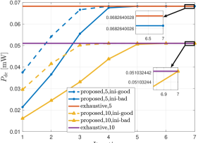
Figure 2: Convergence behavior of proposed algorithm with 5 receivers and 10 receivers.

In the simulation, the WPT receivers are randomly located in a square area with the width of 5m. The transmit power of the WPT transmitter is set to 30dBm. The received RF power at a unit distance is set to 10dBm, i.e., $Q_{0}=10$dBm. In order to evaluate the performance of our iterative algorithm, we compare the results with the optimum obtained by a grid based exhaustive search. The exhaustive search is conducted as follows. First, we define the searching area as $\mathcal{A}:=\{(x,y)|x_{\text{min}}\leq x\leq x_{\text{max}},y_{\text{min}}\leq y\leq y_{\text{max}}\}$. Then, we discretize the area $\mathcal{A}$ into meshes with the resolution of $\xi$ and get a grid based searching area defined as $\tilde{\mathcal{A}}=\{(x_{i},y_{i})|i\in\mathcal{I}\}$, where $(x_{i},y_{i})$ is the $i$-th grid point and $\mathcal{I}$ is the index set of all grid points. Finally, we calculate the minimal harvested DC power among all receivers for each grid point, which results in a set of solutions $\{P_{\text{dc},i}|\forall i\in\mathcal{I}\}$. The result of the exhaustive search is obtained by taking the maximum value among these solutions, i.e., $P^{\star}_{\text{dc}}=\underset{i}{\text{max}}\{P_{\text{dc},i}\}$. In our simulation, the grid resolution is chosen as $\xi=0.001$. The corresponding relative difference between the results at the optimal point of exhaustive search and its adjacent points is with the magnitude of $10^{-7}$, which shows a high accuracy of the chosen resolution.

In Fig. 2 the convergence behavior of the proposed iterative algorithm with 5 and 10 receivers is depicted. For each scenario the iterative algorithm is tested with two initial points. Specifically, one initial point is chosen as the point that is very close to a WPT receiver, denoted as the “ini-bad” in the figure, and another initial point is chosen as the point that is close to the geometry center point of all WPT receivers, denoted as the “ini-good” in the figure. It is observed that the results of both initializations of the proposed iterative algorithm converge to the same stable point which is very close to the global optimum. Moreover, the results also show that with a better initial point, i.e., a point that is close to the optimal point, the iterative algorithm converges within fewer iterations. Nevertheless, the algorithm convergences within less 7 iterations even with a very bad initial point, e.g., a point that is very close to one of the receivers. This shows a good applicability of the proposed iterative algorithm.

V Conclusion

In this work, we addressed the convex property of a nonlinear WPT EH model. We showed that the harvested DC power via the nonlinear model is convex in the reciprocal of the power of the received RF signal. This result indicates that the harvested DC power is convex in the path-loss of the RF signal transmitting link, which facilitates WPT network designs, i.e., resource allocation, WPT devices positioning. As an example, we provide a case study of applying the proved convexity in a WPT transmitter positioning problem. Owning to the convexity, we approximate the non-convex problem and solve it in a interactive manner. The simulation results confirm the converging speed of the interactive algorithm as well as its performance in comparison to the exhaustive search.

References

- [1] H.J. Visser, R.J.M. Vullers, “RF energy harvesting and transport for wireless sensor network applications: principles and requirements,” Proceedings of the IEEE, Vol. 101, No. 6, June 2013
- [2] D. Hwang, D. I. Kim, and T. J. Lee, “Throughput maximization for multiuser MIMO wireless powered communication networks,” IEEE Trans. Veh. Technol., vol. 65, no. 7, pp. 5743–5748, Jul. 2016.
- [3] S. Yin and Z. Qu, “Resource allocation in cooperative networks with wireless information and power transfer,” IEEE Trans. Veh. Technol., vol. 67, no. 1, pp. 718–733, Jan. 2018.
- [4] A. Boaventura, A. Collado, N. B. Carvalho, and A. Georgiadis, “Optimum behavior: Wireless power transmission system design through behavioral models and efficient synthesis techniques,” IEEE Microw. Mag., vol. 14, no. 2, pp. 26–35, Apr. 2013
- [5] B. Clerckx, A. Costanzo, A. Georgiadis, and N.B. Carvalho, “Toward 1G Mobile Power Networks: RF, Signal, and System Designs to Make Smart Objects Autonomous,” IEEE Microw. Mag., vol. 19, no. 6, pp. 69 – 82, Sept./Oct. 2018.
- [6] Y. Zeng, B. Clerckx and R. Zhang, “Communications and Signals Design for Wireless Power Transmission,” IEEE Trans. on Comm, invited paper, Vol 65, No 5, pp 2264 – 2290, May 2017.
- [7] B. Clerckx, R. Zhang, R. Schober, D. W. K. Ng, D. I. Kim, and H. V. Poor, “Fundamentals of Wireless Information and Power Transfer: From RF Energy Harvester Models to Signal and System Designs,” IEEE JSAC, vol. 37, no. 1, pp. 4-33, Jan 2019.
- [8] B. Clerckx and E. Bayguzina, “Waveform Design for Wireless Power Transfer,” IEEE Trans. on Sig. Proc., vol. 64, no. 23, Dec 2016.
- [9] H. Tran, G. Kaddoum and K. T. Truong, ”Resource allocation in SWIPT networks under a nonlinear energy harvesting model: power efficiency, user fairness, and channel nonreciprocity,” IEEE Trans. Veh. Technol., vol. 67, no. 9, pp. 8466-8480, Sept. 2018.
- [10] L. Shi, W. Cheng, Y. Ye, H. Zhang and R. Q. Hu, ”Heterogeneous power-splitting based two-way DF relaying with non-linear energy harvesting,” IEEE GLOBECOM, Abu Dhabi, United Arab Emirates, 2018, pp. 1-7.
- [11] E. Boshkovska, D. W. K. Ng, N. Zlatanov, A. Koelpin and R. Schober, ”Robust resource allocation for MIMO wireless powered communication networks based on a non-linear EH model,” IEEE Trans. Commun., vol. 65, no. 5, pp. 1984-1999, May 2017.
- [12] B. Clerckx and J. Kim, “On the Beneficial Roles of Fading and Transmit Diversity in Wireless Power Transfer with Nonlinear Energy Harvesting,” IEEE Trans. on Wireless Commun., vol. 17, no. 11, pp. 7731 – 7743, Nov. 2018.
- [13] B. Clerckx, “Wireless Information and Power Transfer: Nonlinearity, Waveform Design and Rate-Energy Tradeoff”, IEEE Trans. on Sig Proc., vol 66, no 4, pp 847-862, Feb 2018.
- [14] M. Varasteh, B. Rassouli and B. Clerckx, “Wireless Information and Power Transfer over an AWGN channel: Nonlinearity and Asymmetric Gaussian Signaling”, IEEE ITW 2017.
- [15] M. Varasteh, B. Rassouli, and B. Clerckx, “On Capacity-Achieving Distributions for Complex AWGN Channels under Nonlinear Power Constraints and their Applications to SWIPT,” arXiv:1712.01226
- [16] J. Kim, B. Clerckx, P. D. Mitcheson, “Signal and System Design for Wireless Power Transfer: Prototype, Experiment and Validation” online version, arXiv:1901.01156
- [17] B. R. Marks and G. P. Wright, “A general inner approximation algorithm for nonconvex mathematical programs,” Operations Research, vol. 26, no. 4, pp. 681–683, 1978.