Abstract
Grimmett and McDiarmid suggested a simple heuristic for finding stable sets in random graphs. They showed that the heuristic finds a stable set of size ∼ log 2 n similar-to absent subscript 2 𝑛 \sim\log_{2}n G ( n , 1 / 2 ) 𝐺 𝑛 1 2 G(n,1/2)
1 Introduction
Grimmett and McDiarmid [GM75 ] considered the problem of coloring G ( n , 1 / 2 ) 𝐺 𝑛 1 2 G(n,1/2) log 2 n subscript 2 𝑛 \log_{2}n 2 log 2 n 2 subscript 2 𝑛 2\log_{2}n
Let us briefly indicate how to analyze the algorithm (for more details, consult any lecture notes on the subject). Denote by N k subscript 𝑁 𝑘 N_{k} k 𝑘 k k 𝑘 k 𝔼 [ N k ] ≤ n / 2 k 𝔼 delimited-[] subscript 𝑁 𝑘 𝑛 superscript 2 𝑘 \mathbb{E}[N_{k}]\leq n/2^{k} log 2 n + f ( n ) subscript 2 𝑛 𝑓 𝑛 \log_{2}n+f(n) f ( n ) 𝑓 𝑛 f(n) any function satisfying f ( n ) → ∞ → 𝑓 𝑛 f(n)\to\infty
For the lower bound, let us imagine that there are infinitely many vertices (this idea already appears in [GM75 ] ), let i 0 = 0 subscript 𝑖 0 0 i_{0}=0 i k subscript 𝑖 𝑘 i_{k} k 𝑘 k 1 1 1 i k + 1 − i k ∼ G ( 2 − k ) similar-to subscript 𝑖 𝑘 1 subscript 𝑖 𝑘 𝐺 superscript 2 𝑘 i_{k+1}-i_{k}\sim G(2^{-k}) 2 − k superscript 2 𝑘 2^{-k} k 𝑘 k i k ≤ n subscript 𝑖 𝑘 𝑛 i_{k}\leq n 𝔼 [ i k ] = 2 k − 1 𝔼 delimited-[] subscript 𝑖 𝑘 superscript 2 𝑘 1 \mathbb{E}[i_{k}]=2^{k}-1 log 2 n − f ( n ) subscript 2 𝑛 𝑓 𝑛 \log_{2}n-f(n) f ( n ) 𝑓 𝑛 f(n) any function satisfying f ( n ) → ∞ → 𝑓 𝑛 f(n)\to\infty
Let 𝐤 𝐤 \mathbf{k} 𝐤 − log 2 n 𝐤 subscript 2 𝑛 \mathbf{k}-\log_{2}n 𝐤 𝐤 \mathbf{k} log 2 n subscript 2 𝑛 \log_{2}n { log 2 n } subscript 2 𝑛 \{\log_{2}n\} 𝐤 − log 2 n 𝐤 subscript 2 𝑛 \mathbf{k}-\log_{2}n
Definition 1.1 .
The random variable 𝐇 𝐇 \mathbf{H}
𝐇 = ∑ i = 1 ∞ E ( 2 i ) . 𝐇 superscript subscript 𝑖 1 𝐸 superscript 2 𝑖 \mathbf{H}=\sum_{i=1}^{\infty}E(2^{i}).
(This defines a random variable due to Kolmogorov’s two-series theorem.)
Theorem 1.2 .
For a given n 𝑛 n
p k = Pr [ 𝐤 = k ] , q k = Pr [ n 2 k + 1 ≤ 𝐇 < n 2 k ] . formulae-sequence subscript 𝑝 𝑘 Pr 𝐤 𝑘 subscript 𝑞 𝑘 Pr 𝑛 superscript 2 𝑘 1 𝐇 𝑛 superscript 2 𝑘 p_{k}=\Pr[\mathbf{k}=k],\quad q_{k}=\Pr\left[\frac{n}{2^{k+1}}\leq\mathbf{H}<\frac{n}{2^{k}}\right].
Then we have
∑ k = 0 ∞ | p k − q k | = o ( 1 ) . superscript subscript 𝑘 0 subscript 𝑝 𝑘 subscript 𝑞 𝑘 𝑜 1 \sum_{k=0}^{\infty}|p_{k}-q_{k}|=o(1).
Preliminaries
The Wasserstein distance W 1 ( X , Y ) subscript 𝑊 1 𝑋 𝑌 W_{1}(X,Y) 𝔼 [ | X − Y | ] 𝔼 delimited-[] 𝑋 𝑌 \mathbb{E}[|X-Y|] X , Y 𝑋 𝑌
X,Y W 1 ( X 1 + X 2 , Y 1 + Y 2 ) ≤ W 1 ( X 1 , Y 1 ) + W 1 ( X 2 , Y 2 ) subscript 𝑊 1 subscript 𝑋 1 subscript 𝑋 2 subscript 𝑌 1 subscript 𝑌 2 subscript 𝑊 1 subscript 𝑋 1 subscript 𝑌 1 subscript 𝑊 1 subscript 𝑋 2 subscript 𝑌 2 W_{1}(X_{1}+X_{2},Y_{1}+Y_{2})\leq W_{1}(X_{1},Y_{1})+W_{1}(X_{2},Y_{2})
W 1 ( X , Y ) = ∫ − ∞ ∞ | Pr [ X < t ] − Pr [ Y < t ] | 𝑑 t . subscript 𝑊 1 𝑋 𝑌 superscript subscript Pr 𝑋 𝑡 Pr 𝑌 𝑡 differential-d 𝑡 W_{1}(X,Y)=\int_{-\infty}^{\infty}|\Pr[X<t]-\Pr[Y<t]|\,dt.
The Kolmogorov–Smirnov distance between X 𝑋 X Y 𝑌 Y sup t | Pr [ X < t ] − | P r [ Y < t ] | \sup_{t}|\Pr[X<t]-|Pr[Y<t]| Y 𝑌 Y C 𝐶 C X 𝑋 X Y 𝑌 Y 2 C W 1 ( X , Y ) 2 𝐶 subscript 𝑊 1 𝑋 𝑌 2\sqrt{CW_{1}(X,Y)}
2 Proof
Recall that 𝐤 𝐤 \mathbf{k}
Lemma 2.1 .
Pr [ 𝐤 < k ] = Pr [ G ( 1 ) + G ( 1 / 2 ) + ⋯ + G ( 1 / 2 k − 1 ) > n ] = Pr [ G ( 1 / 2 ) + ⋯ + G ( 1 / 2 k − 1 ) ≥ n ] . Pr 𝐤 𝑘 Pr 𝐺 1 𝐺 1 2 ⋯ 𝐺 1 superscript 2 𝑘 1 𝑛 Pr 𝐺 1 2 ⋯ 𝐺 1 superscript 2 𝑘 1 𝑛 \Pr[\mathbf{k}<k]=\Pr[G(1)+G(1/2)+\cdots+G(1/2^{k-1})>n]=\Pr[G(1/2)+\cdots+G(1/2^{k-1})\geq n].
Our main idea is to rewrite this formula as follows:
Pr [ 𝐤 < k ] = Pr [ G ( 1 / 2 k − 1 ) n + G ( 1 / 2 k − 2 ) n + ⋯ + G ( 1 / 2 ) n ≥ 1 ] . Pr 𝐤 𝑘 Pr 𝐺 1 superscript 2 𝑘 1 𝑛 𝐺 1 superscript 2 𝑘 2 𝑛 ⋯ 𝐺 1 2 𝑛 1 \Pr[\mathbf{k}<k]=\Pr\left[\frac{G(1/2^{k-1})}{n}+\frac{G(1/2^{k-2})}{n}+\cdots+\frac{G(1/2)}{n}\geq 1\right]. (1)
It is known that the distribution G ( c / n ) / n 𝐺 𝑐 𝑛 𝑛 G(c/n)/n E ( c ) 𝐸 𝑐 E(c) W 1 subscript 𝑊 1 W_{1}
Lemma 2.2 .
If p ≤ 1 / 2 𝑝 1 2 p\leq 1/2
W 1 ( G ( p ) / n , E ( p n ) ) = O ( 1 n ) . subscript 𝑊 1 𝐺 𝑝 𝑛 𝐸 𝑝 𝑛 𝑂 1 𝑛 W_{1}(G(p)/n,E(pn))=O\left(\frac{1}{n}\right).
Proof.
Let X = ⌈ E ( p n ) n ⌉ 𝑋 𝐸 𝑝 𝑛 𝑛 X=\lceil E(pn)n\rceil t 𝑡 t
Pr [ X ≥ t ] = Pr [ E ( p n ) > ( t − 1 ) / n ] = e − p ( t − 1 ) . Pr 𝑋 𝑡 Pr 𝐸 𝑝 𝑛 𝑡 1 𝑛 superscript 𝑒 𝑝 𝑡 1 \Pr[X\geq t]=\Pr[E(pn)>(t-1)/n]=e^{-p(t-1)}.
In contrast,
Pr [ G ( p ) ≥ t ] = ( 1 − p ) t − 1 . Pr 𝐺 𝑝 𝑡 superscript 1 𝑝 𝑡 1 \Pr[G(p)\geq t]=(1-p)^{t-1}.
By construction, W 1 ( X / n , E ( p n ) ) ≤ 1 / n subscript 𝑊 1 𝑋 𝑛 𝐸 𝑝 𝑛 1 𝑛 W_{1}(X/n,E(pn))\leq 1/n
W 1 ( G ( p ) / n , E ( p n ) ) ≤ 1 n + W 1 ( G ( p ) / n , X / n ) ≤ 1 n + ∫ 0 ∞ | Pr [ G ( p ) / n ≥ s ] − Pr [ X / n ≥ s ] | 𝑑 s = 1 n + 1 n ∑ r = 0 ∞ | Pr [ G ( p ) ≥ r ] − Pr [ X ≥ r ] | = 1 n + 1 n ∑ t = 1 ∞ | ( 1 − p ) t − e − p t | . subscript 𝑊 1 𝐺 𝑝 𝑛 𝐸 𝑝 𝑛 1 𝑛 subscript 𝑊 1 𝐺 𝑝 𝑛 𝑋 𝑛 1 𝑛 superscript subscript 0 Pr 𝐺 𝑝 𝑛 𝑠 Pr 𝑋 𝑛 𝑠 differential-d 𝑠 1 𝑛 1 𝑛 superscript subscript 𝑟 0 Pr 𝐺 𝑝 𝑟 Pr 𝑋 𝑟 1 𝑛 1 𝑛 superscript subscript 𝑡 1 superscript 1 𝑝 𝑡 superscript 𝑒 𝑝 𝑡 W_{1}(G(p)/n,E(pn))\leq\frac{1}{n}+W_{1}(G(p)/n,X/n)\leq\frac{1}{n}+\int_{0}^{\infty}|\Pr[G(p)/n\geq s]-\Pr[X/n\geq s]|\,ds=\\
\frac{1}{n}+\frac{1}{n}\sum_{r=0}^{\infty}|\Pr[G(p)\geq r]-\Pr[X\geq r]|=\frac{1}{n}+\frac{1}{n}\sum_{t=1}^{\infty}|(1-p)^{t}-e^{-pt}|.
Since p ≤ 1 / 2 𝑝 1 2 p\leq 1/2 − p − O ( p 2 ) ≤ log ( 1 − p ) ≤ − p 𝑝 𝑂 superscript 𝑝 2 1 𝑝 𝑝 -p-O(p^{2})\leq\log(1-p)\leq-p
e − p t − O ( p 2 t ) ≤ ( 1 − p ) t ≤ e − p t . superscript 𝑒 𝑝 𝑡 𝑂 superscript 𝑝 2 𝑡 superscript 1 𝑝 𝑡 superscript 𝑒 𝑝 𝑡 e^{-pt-O(p^{2}t)}\leq(1-p)^{t}\leq e^{-pt}.
Therefore
| ( 1 − p ) t − e − p t | = e − p t ( 1 − e − O ( p 2 t ) ) = O ( p 2 t e − p t ) . superscript 1 𝑝 𝑡 superscript 𝑒 𝑝 𝑡 superscript 𝑒 𝑝 𝑡 1 superscript 𝑒 𝑂 superscript 𝑝 2 𝑡 𝑂 superscript 𝑝 2 𝑡 superscript 𝑒 𝑝 𝑡 |(1-p)^{t}-e^{-pt}|=e^{-pt}(1-e^{-O(p^{2}t)})=O(p^{2}te^{-pt}).
We can thus bound
∑ t = 1 ∞ | ( 1 − p ) t − e − p t | ≤ O ( p 2 ) ∑ t = 1 ∞ t e p t = O ( p 2 e p ( e p − 1 ) 2 ) = O ( 1 ) . ∎ superscript subscript 𝑡 1 superscript 1 𝑝 𝑡 superscript 𝑒 𝑝 𝑡 𝑂 superscript 𝑝 2 superscript subscript 𝑡 1 𝑡 superscript 𝑒 𝑝 𝑡 𝑂 superscript 𝑝 2 superscript 𝑒 𝑝 superscript superscript 𝑒 𝑝 1 2 𝑂 1 \sum_{t=1}^{\infty}|(1-p)^{t}-e^{-pt}|\leq O(p^{2})\sum_{t=1}^{\infty}\frac{t}{e^{pt}}=O\left(\frac{p^{2}e^{p}}{(e^{p}-1)^{2}}\right)=O(1).\qed
Since W 1 subscript 𝑊 1 W_{1}
Lemma 2.3 .
Let 𝐆 𝐆 \mathbf{G} 1
W 1 ( n 2 k 𝐆 , 𝐇 ) = O ( k 2 k ) . subscript 𝑊 1 𝑛 superscript 2 𝑘 𝐆 𝐇 𝑂 𝑘 superscript 2 𝑘 W_{1}\left(\frac{n}{2^{k}}\mathbf{G},\mathbf{H}\right)=O\left(\frac{k}{2^{k}}\right).
Proof.
Lemma 2.2
W 1 ( 𝐆 , E ( n / 2 k − 1 ) + ⋯ + E ( n / 2 ) ) = O ( k n ) , subscript 𝑊 1 𝐆 𝐸 𝑛 superscript 2 𝑘 1 ⋯ 𝐸 𝑛 2 𝑂 𝑘 𝑛 W_{1}(\mathbf{G},E(n/2^{k-1})+\cdots+E(n/2))=O\left(\frac{k}{n}\right),
which implies that
W 1 ( n 2 k 𝐆 , E ( 2 ) + ⋯ + E ( 2 k − 1 ) ) = O ( k 2 k ) . subscript 𝑊 1 𝑛 superscript 2 𝑘 𝐆 𝐸 2 ⋯ 𝐸 superscript 2 𝑘 1 𝑂 𝑘 superscript 2 𝑘 W_{1}\left(\frac{n}{2^{k}}\mathbf{G},E(2)+\cdots+E(2^{k-1})\right)=O\left(\frac{k}{2^{k}}\right).
On the other hand,
W 1 ( ∑ ℓ = k ∞ E ( 2 ℓ ) , 𝟎 ) = 𝔼 [ ∑ ℓ = k ∞ E ( 2 ℓ ) ] = 1 2 k − 1 , subscript 𝑊 1 superscript subscript ℓ 𝑘 𝐸 superscript 2 ℓ 0 𝔼 delimited-[] superscript subscript ℓ 𝑘 𝐸 superscript 2 ℓ 1 superscript 2 𝑘 1 W_{1}\left(\sum_{\ell=k}^{\infty}E(2^{\ell}),\mathbf{0}\right)=\mathbb{E}\left[\sum_{\ell=k}^{\infty}E(2^{\ell})\right]=\frac{1}{2^{k-1}},
where 𝟎 0 \mathbf{0}
In order to convert this bound to a bound on the Kolmogorov–Smirnov distance, we need to know that 𝐇 𝐇 \mathbf{H}
Lemma 2.4 .
The random variable 𝐇 𝐇 \mathbf{H} f 𝑓 f
f ( x ) = 2 C − 1 ∑ i = 1 ∞ ( − 1 ) i − 1 e − 2 i x ∏ r = 1 i − 1 2 2 r − 1 , where C = ∏ s = 1 ∞ ( 1 − 2 − s ) > 0 . formulae-sequence 𝑓 𝑥 2 superscript 𝐶 1 superscript subscript 𝑖 1 superscript 1 𝑖 1 superscript 𝑒 superscript 2 𝑖 𝑥 superscript subscript product 𝑟 1 𝑖 1 2 superscript 2 𝑟 1 where 𝐶 superscript subscript product 𝑠 1 1 superscript 2 𝑠 0 f(x)=2C^{-1}\sum_{i=1}^{\infty}(-1)^{i-1}e^{-2^{i}x}\prod_{r=1}^{i-1}\frac{2}{2^{r}-1},\text{ where }C=\prod_{s=1}^{\infty}(1-2^{-s})>0.
(The constant C 𝐶 C n × n 𝑛 𝑛 n\times n 𝐺𝐹 ( 2 ) 𝐺𝐹 2 \mathit{GF}(2)
Proof.
Let 𝐇 ( ℓ ) = ∑ i = 1 ℓ E ( 2 i ) superscript 𝐇 ℓ superscript subscript 𝑖 1 ℓ 𝐸 superscript 2 𝑖 \mathbf{H}^{(\ell)}=\sum_{i=1}^{\ell}E(2^{i}) 𝐇 ( ℓ ) superscript 𝐇 ℓ \mathbf{H}^{(\ell)}
f ℓ ( x ) = ∑ i = 1 ℓ 2 i e − 2 i x K ℓ , i , where K ℓ , i = ∏ j = 1 j ≠ i ℓ 2 j 2 j − 2 i . formulae-sequence subscript 𝑓 ℓ 𝑥 superscript subscript 𝑖 1 ℓ superscript 2 𝑖 superscript 𝑒 superscript 2 𝑖 𝑥 subscript 𝐾 ℓ 𝑖
where subscript 𝐾 ℓ 𝑖
superscript subscript product 𝑗 1 𝑗 𝑖
ℓ superscript 2 𝑗 superscript 2 𝑗 superscript 2 𝑖 f_{\ell}(x)=\sum_{i=1}^{\ell}2^{i}e^{-2^{i}x}K_{\ell,i},\text{ where }K_{\ell,i}=\prod_{\begin{subarray}{c}j=1\\
j\neq i\end{subarray}}^{\ell}\frac{2^{j}}{2^{j}-2^{i}}.
Note that
K ℓ , i = ( − 1 ) i − 1 ∏ j = 1 i − 1 1 2 i − j − 1 × ∏ j = i + 1 ℓ 1 1 − 2 i − j = ( − 1 ) i − 1 ∏ r = 1 i − 1 1 2 r − 1 × ∏ s = 1 ℓ − i 1 1 − 2 − s . subscript 𝐾 ℓ 𝑖
superscript 1 𝑖 1 superscript subscript product 𝑗 1 𝑖 1 1 superscript 2 𝑖 𝑗 1 superscript subscript product 𝑗 𝑖 1 ℓ 1 1 superscript 2 𝑖 𝑗 superscript 1 𝑖 1 superscript subscript product 𝑟 1 𝑖 1 1 superscript 2 𝑟 1 superscript subscript product 𝑠 1 ℓ 𝑖 1 1 superscript 2 𝑠 K_{\ell,i}=(-1)^{i-1}\prod_{j=1}^{i-1}\frac{1}{2^{i-j}-1}\times\prod_{j=i+1}^{\ell}\frac{1}{1-2^{i-j}}=(-1)^{i-1}\prod_{r=1}^{i-1}\frac{1}{2^{r}-1}\times\prod_{s=1}^{\ell-i}\frac{1}{1-2^{-s}}.
We can therefore write
f ℓ ( x ) = ∑ i = 1 ℓ 2 e − 2 i x × ( − 1 ) i − 1 ∏ r = 1 i − 1 2 2 r − 1 × ∏ s = 1 ℓ − i 1 1 − 2 − s . subscript 𝑓 ℓ 𝑥 superscript subscript 𝑖 1 ℓ 2 superscript 𝑒 superscript 2 𝑖 𝑥 superscript 1 𝑖 1 superscript subscript product 𝑟 1 𝑖 1 2 superscript 2 𝑟 1 superscript subscript product 𝑠 1 ℓ 𝑖 1 1 superscript 2 𝑠 f_{\ell}(x)=\sum_{i=1}^{\ell}2e^{-2^{i}x}\times(-1)^{i-1}\prod_{r=1}^{i-1}\frac{2}{2^{r}-1}\times\prod_{s=1}^{\ell-i}\frac{1}{1-2^{-s}}.
This allows us to bound
| f ℓ ( x ) | ≤ 2 C − 1 e − 2 x ∑ i = 1 ℓ ∏ r = 1 i − 1 2 2 r − 1 , subscript 𝑓 ℓ 𝑥 2 superscript 𝐶 1 superscript 𝑒 2 𝑥 superscript subscript 𝑖 1 ℓ superscript subscript product 𝑟 1 𝑖 1 2 superscript 2 𝑟 1 |f_{\ell}(x)|\leq 2C^{-1}e^{-2x}\sum_{i=1}^{\ell}\prod_{r=1}^{i-1}\frac{2}{2^{r}-1},
where C 𝐶 C | f ℓ ( x ) | = O ( e − 2 x ) subscript 𝑓 ℓ 𝑥 𝑂 superscript 𝑒 2 𝑥 |f_{\ell}(x)|=O(e^{-2x}) ℓ ℓ \ell
Armed with this information, we can finally estimate Pr [ 𝐤 < k ] Pr 𝐤 𝑘 \Pr[\mathbf{k}<k]
Lemma 2.5 .
Pr [ 𝐤 < k ] = Pr [ 𝐇 ≥ n 2 k ] ± O ( k 2 k ) . Pr 𝐤 𝑘 plus-or-minus Pr 𝐇 𝑛 superscript 2 𝑘 𝑂 𝑘 superscript 2 𝑘 \Pr[\mathbf{k}<k]=\Pr\left[\mathbf{H}\geq\frac{n}{2^{k}}\right]\pm O\left(\sqrt{\frac{k}{2^{k}}}\right).
Proof.
Since 𝐇 𝐇 \mathbf{H} Lemma 2.4 n 2 k 𝐆 𝑛 superscript 2 𝑘 𝐆 \tfrac{n}{2^{k}}\mathbf{G} 𝐇 𝐇 \mathbf{H} O ( W 1 ( n 2 k 𝐆 , 𝐇 ) ) = O ( k / 2 k ) 𝑂 subscript 𝑊 1 𝑛 superscript 2 𝑘 𝐆 𝐇 𝑂 𝑘 superscript 2 𝑘 O(\sqrt{W_{1}(\tfrac{n}{2^{k}}\mathbf{G},\mathbf{H})})=O(\sqrt{k/2^{k}}) Lemma 2.3
Pr [ 𝐤 < k ] = Pr [ n 2 k 𝐆 ≥ n 2 k ] = Pr [ 𝐇 ≥ n 2 k ] ± O ( k 2 k ) . ∎ Pr 𝐤 𝑘 Pr 𝑛 superscript 2 𝑘 𝐆 𝑛 superscript 2 𝑘 plus-or-minus Pr 𝐇 𝑛 superscript 2 𝑘 𝑂 𝑘 superscript 2 𝑘 \Pr[\mathbf{k}<k]=\Pr\left[\frac{n}{2^{k}}\mathbf{G}\geq\frac{n}{2^{k}}\right]=\Pr\left[\mathbf{H}\geq\frac{n}{2^{k}}\right]\pm O\left(\sqrt{\frac{k}{2^{k}}}\right).\qed
Lemma 2.5 k 𝑘 k
Pr [ 𝐤 = k ] = Pr [ 𝐤 < k + 1 ] − Pr [ 𝐤 < k ] = Pr [ n 2 k + 1 ≤ 𝐇 < n 2 k ] ± O ( k 2 k ) . Pr 𝐤 𝑘 Pr 𝐤 𝑘 1 Pr 𝐤 𝑘 plus-or-minus Pr 𝑛 superscript 2 𝑘 1 𝐇 𝑛 superscript 2 𝑘 𝑂 𝑘 superscript 2 𝑘 \Pr[\mathbf{k}=k]=\Pr[\mathbf{k}<k+1]-\Pr[\mathbf{k}<k]=\Pr\left[\frac{n}{2^{k+1}}\leq\mathbf{H}<\frac{n}{2^{k}}\right]\pm O\left(\sqrt{\frac{k}{2^{k}}}\right).
This implies that
∑ k = ℓ ∞ | Pr [ 𝐤 = k ] − Pr [ n 2 k + 1 ≤ 𝐇 < n 2 k ] | = O ( ℓ 2 ℓ ) . superscript subscript 𝑘 ℓ Pr 𝐤 𝑘 Pr 𝑛 superscript 2 𝑘 1 𝐇 𝑛 superscript 2 𝑘 𝑂 ℓ superscript 2 ℓ \sum_{k=\ell}^{\infty}\left|\Pr[\mathbf{k}=k]-\Pr\left[\frac{n}{2^{k+1}}\leq\mathbf{H}<\frac{n}{2^{k}}\right]\right|=O\left(\sqrt{\frac{\ell}{2^{\ell}}}\right).
Lemma 2.1
Pr [ 𝐤 < ℓ ] = Pr [ G ( 1 / 2 ) + ⋯ + G ( 1 / 2 ℓ − 1 ) ≥ n ] ≤ 𝔼 [ G ( 1 / 2 ) + ⋯ + G ( 1 / 2 ℓ − 1 ) ] n < 2 ℓ n , Pr 𝐤 ℓ Pr 𝐺 1 2 ⋯ 𝐺 1 superscript 2 ℓ 1 𝑛 𝔼 delimited-[] 𝐺 1 2 ⋯ 𝐺 1 superscript 2 ℓ 1 𝑛 superscript 2 ℓ 𝑛 \Pr[\mathbf{k}<\ell]=\Pr[G(1/2)+\cdots+G(1/2^{\ell-1})\geq n]\leq\frac{\mathbb{E}[G(1/2)+\cdots+G(1/2^{\ell-1})]}{n}<\frac{2^{\ell}}{n},
and so choosing ℓ := 2 3 log 2 n assign ℓ 2 3 subscript 2 𝑛 \ell:=\tfrac{2}{3}\log_{2}n
Pr [ 𝐤 < ℓ ] ≤ 1 n 1 / 3 . Pr 𝐤 ℓ 1 superscript 𝑛 1 3 \Pr[\mathbf{k}<\ell]\leq\frac{1}{n^{1/3}}.
Lemma 2.5
Pr [ 𝐇 ≥ n 2 ℓ ] = O ( log n n 1 / 3 ) , Pr 𝐇 𝑛 superscript 2 ℓ 𝑂 𝑛 superscript 𝑛 1 3 \Pr\left[\mathbf{H}\geq\frac{n}{2^{\ell}}\right]=O\left(\frac{\sqrt{\log n}}{n^{1/3}}\right),
and so
∑ k = 0 ℓ − 1 | Pr [ 𝐤 = k ] − Pr [ n 2 k + 1 ≤ 𝐇 < n 2 k ] | ≤ ∑ k = 0 ℓ − 1 ( Pr [ 𝐤 = k ] + Pr [ n 2 k + 1 ≤ 𝐇 < n 2 k ] ) = O ( log n n 1 / 3 ) . superscript subscript 𝑘 0 ℓ 1 Pr 𝐤 𝑘 Pr 𝑛 superscript 2 𝑘 1 𝐇 𝑛 superscript 2 𝑘 superscript subscript 𝑘 0 ℓ 1 Pr 𝐤 𝑘 Pr 𝑛 superscript 2 𝑘 1 𝐇 𝑛 superscript 2 𝑘 𝑂 𝑛 superscript 𝑛 1 3 \sum_{k=0}^{\ell-1}\left|\Pr[\mathbf{k}=k]-\Pr\left[\frac{n}{2^{k+1}}\leq\mathbf{H}<\frac{n}{2^{k}}\right]\right|\leq\sum_{k=0}^{\ell-1}\left(\Pr[\mathbf{k}=k]+\Pr\left[\frac{n}{2^{k+1}}\leq\mathbf{H}<\frac{n}{2^{k}}\right]\right)=O\left(\frac{\sqrt{\log n}}{n^{1/3}}\right).
In total, we conclude that
∑ k = 0 ∞ | Pr [ 𝐤 = k ] − Pr [ n 2 k + 1 ≤ 𝐇 < n 2 k ] | = O ( log n n 1 / 3 ) . ∎ superscript subscript 𝑘 0 Pr 𝐤 𝑘 Pr 𝑛 superscript 2 𝑘 1 𝐇 𝑛 superscript 2 𝑘 𝑂 𝑛 superscript 𝑛 1 3 \sum_{k=0}^{\infty}\left|\Pr[\mathbf{k}=k]-\Pr\left[\frac{n}{2^{k+1}}\leq\mathbf{H}<\frac{n}{2^{k}}\right]\right|=O\left(\frac{\sqrt{\log n}}{n^{1/3}}\right).\qed
We can also express Theorem 1.2 𝐤 𝐤 \mathbf{k}
Let θ = { log 2 n } = log 2 n − ⌊ log 2 n ⌋ 𝜃 subscript 2 𝑛 subscript 2 𝑛 subscript 2 𝑛 \theta=\{\log_{2}n\}=\log_{2}n-\lfloor\log_{2}n\rfloor k = ⌊ log 2 n ⌋ + c 𝑘 subscript 2 𝑛 𝑐 k=\lfloor\log_{2}n\rfloor+c n / 2 k = 2 θ − c 𝑛 superscript 2 𝑘 superscript 2 𝜃 𝑐 n/2^{k}=2^{\theta-c} q k subscript 𝑞 𝑘 q_{k} Theorem 1.2
Pr [ 2 − ( c + 1 ) ≤ 2 − θ 𝐇 < 2 − c ] = Pr [ 2 − ( c + 1 ) < 2 − θ 𝐇 ≤ 2 − c ] = Pr [ ⌊ log 2 ( 1 / 𝐇 ) + θ ⌋ = c ] . Pr superscript 2 𝑐 1 superscript 2 𝜃 𝐇 superscript 2 𝑐 Pr superscript 2 𝑐 1 superscript 2 𝜃 𝐇 superscript 2 𝑐 Pr subscript 2 1 𝐇 𝜃 𝑐 \Pr[2^{-(c+1)}\leq 2^{-\theta}\mathbf{H}<2^{-c}]=\Pr[2^{-(c+1)}<2^{-\theta}\mathbf{H}\leq 2^{-c}]=\Pr[\lfloor\log_{2}(1/\mathbf{H})+\theta\rfloor=c].
Therefore we obtain the following corollary:
Corollary 2.6 .
For a given n 𝑛 n θ = { log 2 n } 𝜃 subscript 2 𝑛 \theta=\{\log_{2}n\}
𝐡 = ⌊ log 2 ( 1 / 𝐇 ) + θ ⌋ . 𝐡 subscript 2 1 𝐇 𝜃 \mathbf{h}=\lfloor\log_{2}(1/\mathbf{H})+\theta\rfloor.
The variation distance between 𝐤 𝐤 \mathbf{k} 𝐡 𝐡 \mathbf{h} O ~ ( 1 / n 1 / 3 ) ~ 𝑂 1 superscript 𝑛 1 3 \tilde{O}(1/n^{1/3})
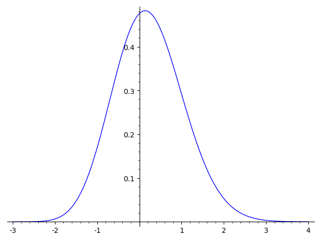
The random variable log 2 ( 1 / 𝐇 ) subscript 2 1 𝐇 \log_{2}(1/\mathbf{H})
g ( y ) = ( 2 C − 1 ln 2 ) 2 − y ∑ i = 1 ∞ ( − 1 ) i − 1 e − 2 i − y ∏ r = 1 i − 1 2 2 r − 1 , 𝑔 𝑦 2 superscript 𝐶 1 2 superscript 2 𝑦 superscript subscript 𝑖 1 superscript 1 𝑖 1 superscript 𝑒 superscript 2 𝑖 𝑦 superscript subscript product 𝑟 1 𝑖 1 2 superscript 2 𝑟 1 g(y)=(2C^{-1}\ln 2)2^{-y}\sum_{i=1}^{\infty}(-1)^{i-1}e^{-2^{i-y}}\prod_{r=1}^{i-1}\frac{2}{2^{r}-1},
and is plotted in Fig. 1
Figure 1: Density of log 2 ( 1 / 𝐇 ) subscript 2 1 𝐇 \log_{2}(1/\mathbf{H})
3 Applications
Integrating the formula given in Lemma 2.4 Lemma 2.5
P r [ 𝐤 = k ] ≈ C − 1 ∑ i = 1 ∞ ( − 1 ) i − 1 ( e − n 2 i − k − 1 − e − n 2 i − k ) ∏ r = 1 i − 1 1 2 r − 1 , 𝑃 𝑟 delimited-[] 𝐤 𝑘 superscript 𝐶 1 superscript subscript 𝑖 1 superscript 1 𝑖 1 superscript 𝑒 𝑛 superscript 2 𝑖 𝑘 1 superscript 𝑒 𝑛 superscript 2 𝑖 𝑘 superscript subscript product 𝑟 1 𝑖 1 1 superscript 2 𝑟 1 Pr[\mathbf{k}=k]\approx C^{-1}\sum_{i=1}^{\infty}(-1)^{i-1}\left(e^{-n2^{i-k-1}}-e^{-n2^{i-k}}\right)\prod_{r=1}^{i-1}\frac{1}{2^{r}-1},
where the error is O ( k / 2 k ) 𝑂 𝑘 superscript 2 𝑘 O(k/2^{k}) k = log 2 n + c 𝑘 subscript 2 𝑛 𝑐 k=\log_{2}n+c
P r [ 𝐤 = log 2 n + c ] ≈ C − 1 ∑ i = 1 ∞ ( − 1 ) i − 1 ( e − 2 i − c − 1 − e − 2 i − c ) ∏ r = 1 i − 1 1 2 r − 1 . 𝑃 𝑟 delimited-[] 𝐤 subscript 2 𝑛 𝑐 superscript 𝐶 1 superscript subscript 𝑖 1 superscript 1 𝑖 1 superscript 𝑒 superscript 2 𝑖 𝑐 1 superscript 𝑒 superscript 2 𝑖 𝑐 superscript subscript product 𝑟 1 𝑖 1 1 superscript 2 𝑟 1 Pr[\mathbf{k}=\log_{2}n+c]\approx C^{-1}\sum_{i=1}^{\infty}(-1)^{i-1}\left(e^{-2^{i-c-1}}-e^{-2^{i-c}}\right)\prod_{r=1}^{i-1}\frac{1}{2^{r}-1}.
Using this, we can calculate the limiting distribution of 𝐤 𝐤 \mathbf{k} { log 2 n } subscript 2 𝑛 \{\log_{2}n\} n 𝑛 n 2 2 2
c lim Pr [ 𝐤 = log 2 n + c ] − 4 0.000000389680708123307 − 3 0.00116084271918975 − 2 0.0610996920580558 − 1 0.343335642221465 0 0.420730421531672 1 0.153255882765631 2 0.0194547690538043 3 0.000943671851018291 4 0.0000185343323798604 5 0.000000153237063593714 𝑐 Pr 𝐤 subscript 2 𝑛 𝑐 missing-subexpression missing-subexpression 4 0.000000389680708123307 3 0.00116084271918975 2 0.0610996920580558 1 0.343335642221465 0 0.420730421531672 1 0.153255882765631 2 0.0194547690538043 3 0.000943671851018291 4 0.0000185343323798604 5 0.000000153237063593714 \begin{array}[]{r|l}c&\lim\Pr[\mathbf{k}=\log_{2}n+c]\\
\hline\cr-4&0.000000389680708123307\\
-3&0.00116084271918975\\
-2&0.0610996920580558\\
-1&0.343335642221465\\
0&0.420730421531672\\
1&0.153255882765631\\
2&0.0194547690538043\\
3&0.000943671851018291\\
4&0.0000185343323798604\\
5&0.000000153237063593714\end{array}
In this case, the expected deviation of 𝐤 𝐤 \mathbf{k} log 2 n subscript 2 𝑛 \log_{2}n − 0.273947769982407 0.273947769982407 -0.273947769982407 𝐤 𝐤 \mathbf{k} 0.763009254799132 0.763009254799132 0.763009254799132