Competition between tenants with strategic resource allocation in 5G network slicing

Abstract

We propose and analyze a business model for 5G operators. Each operator is entitled to a share of a network operated by an Infrastructure Provider (InP) and use network slicing mechanisms to request network resources as needed for service provision. The network operators become Network Slice Tenants (NSTs). The InP performs the resource allocation based on a vector of weights chosen strategically by each NST. The weights distribute the NST’s share of resources between its subscribers in each cell. We propose a strategy profile in which the NST chooses weights equal to the product of its share by the ratio between the total number of subscribers in the cell and the total number of subscribers in the network. We characterize the proposed solution in terms of subscription ratios and fractions of subscribers, for different cell capacities and user sensitivities. The proposed solution provides the exact values for the Nash equilibrium if the cells are homogeneous in terms of normalized capacity, which is a measure of the total amount of resources available in the cell. Otherwise, if the cells are heterogeneous, it provides an accurate approximation. We quantify the deviation from the equilibrium and conclude that it is highly accurate.

I Introduction

The current mobile network architecture utilizes a relatively monolithic access and transport framework to accommodate a variety of services such as mobile traffic for smart phones, OTT content, feature phones, data cards, and embedded M2M devices. It is anticipated that this architecture will not be flexible and scalable enough to support the coming 5G network, which demands very diverse use cases and sometimes extreme requirements—in terms of performance, scalability and availability. Furthermore, the introduction of new network services should be made more efficiently [1].

In the above scenario, network slicing is gaining an increasing importance as an effective way to introduce flexibility in the management of network resources. A network slice is a collection of network resources, selected in order to satisfy the requirements (e.g. in terms of QoS) of the service(s) to be provided by the slice. An enabling aspect of network slicing is virtualization. Virtualization of network resources allows operators to share the same physical resource in a flexible and dynamic manner to exploit the available resources more efficiently [2].

Within the above context, we envision a scenario where a set of network operators use network slicing mechanisms to request network resources as needed for service provision. The InP is responsible for the network operation and maintenance, while the network operators become Network Slice Tenants (NSTs) . The NSTs are entitled to a share of the network resources. This entitlement may result from diverse scenario, e.g., the operators owned the networks and decided to pool the networks and outsource their operation to and InP.

We propose a business model where the NSTs provide service to end users. This service may be characterized by a series of performance constraints (e.g., transmission rate and delay) and each NST gets revenues from its subscribers. In order to support the service, the NSTs request dynamically access and core network resources from an InP. The InP works as a supporting unit to the NSTs.

Our work analyzes how independent NSTs compete against each other following the business model described above. We show that the strategic interaction between the NSTs both in the provision of the service and in the slicing of the network can be modeled as a game, where the strategy is a weighted distribution of the NST’s share of the resources between the cells. A solution for the Nash equilibrium is proposed in which the NST chooses weights equal to the product of its share by the ratio between the total number of subscribers in the cell and the total number of subscribers in the network. We characterize the proposed solution for different cell capacities and user sensitivities. The proposed solution provides the exact values at the equilibrium if the cells are homogeneous in terms of normalized capacity, which is a measure of the available resources in the cell normalized to the service price, the number of users and the no-subscription option valuation. Otherwise, if the cells are heterogeneous, it provides an accurate approximation of the equilibrium. We quantify the deviation from the equilibrium and conclude that it is highly accurate.

The paper is structured as follows. In Section II, the model for the NSTs, the users, and the InP is described. In Section III, a strategic game is formulated for the interaction between the NSTs, a solution for the Nash equilibrium is proposed and its exactness is discussed. In Section IV, we characterize the solution and quantify the exactness of the proposed solution. And finally, Section V draws the conclusions.

I-A Related work

This work draws on previous works on the provision of services based on different kind of resources, e.g., spectrum [5], sensing measures [6], general data [7].

As far as the resource allocation is concerned, we are indebted to the seminal proposal made by I. Fisher. The Fisher market is one of the most fundamental models within mathematical economics [8]. The basic setting is that of a set of buyers aiming to purchase multiple goods in a way that maximizes their utility subject to budget constraints. The outcome where supply equals demand is known as market equilibrium, and has the property that the buyers spend their entire budgets, all the goods are sold, and the bundle purchased by each buyer maximizes his utility (given his budget and the equilibrium prices of the goods). A market equilibrium is guaranteed to exist under mild conditions. This model has been borrowed by recent proposals on resource allocation mechanisms. In [9], the allocation of computational resources are analyzed, where the budget may have a monetary interpretation. In [10], radio network resources are allocated between network slices, and the budget derives from an initial lease of resources from the NSTs to a common network pool operated by the InP. The above allocation model and mechanism results in a non-efficient allocation when the users act in a strategic manner[9].

Our work focuses on the allocation of 5G network resources that are procured by the tenants through network slicing. We borrow the ideas from the Fisher market model, as in [10]. We are also indebted to the work in [10] and [11] in that the allocation is of a hierarchical nature, where the NSTs are involved in the allocation—as opposed to a centralized scheme, where the InP decides and executes the complete allocation to all users. However, our work differs importantly from these two previous works in that we model the NSTs and the users as different agents with their particular incentives, which are the profits and the user utility, respectively. In [10] and [11], each NST operates as a proxy of its subscribers; this may fail to properly model the NST’s incentives and the corresponding business model. This difference has also an important implication in the user behavior modeling: while in our work the number of subscribers for each NST depends on the NSTs allocation decision, in [10] and [11], it is independent from it, since the number of subscribers is fixed a priori as a parameter.

II Model

In this section, we propose a model amenable for the analysis of the service provision by NSTs, within a network slicing framework.

II-A System model

A network consists of a set of resources $\mathcal{B}$ managed by an InP and leased by a set $\mathcal{S}$ of NSTs. We focus on mobile service operators and, specifically, on the radio access network, so that each element of $\mathcal{B}$ may represent the radio resources of a cell in the network.

The resources leased by the NSTs are used to deliver service to a set $\mathcal{U}$ of users. We define the following subsets of users: $\mathcal{U}^{(j)}$, the users in cell $j$; $\mathcal{U}_{i}$, the subscribers of NST $i$; and $\mathcal{U}^{(j)}_{i}=\mathcal{U}^{(j)}\cap\mathcal{U}_{i}$, the subscribers of NST $i$ in cell $j$.

NST $i$ is entitled to a share $s_{i}$ of the total amount of resources available in the network, such that $\sum_{i\in\mathcal{S}}s_{i}=1$.

The NST allocates the resource for providing service to its subscribers in the following way. NST $i$ distributes its share among its subscribers, assigning a weight $\omega^{(j)}_{i}$ to $\mathcal{U}^{(j)}_{i}$, such that $\omega^{(j)}_{i}>0$ and $\sum_{j\in\mathcal{B}}\omega^{(j)}_{i}=s_{i}\leq 1$. The weight assignment decision is notified to the InP, who proceeds to perform the actual resource allocation in each individual cell. The InP allocates an amount of resources to the set $\mathcal{U}^{(j)}_{i}$ given by

$$R^{(j)}_{i}=\frac{\omega^{(j)}_{i}}{\sum_{t\in\mathcal{S}}\omega^{(j)}_{t}}c^{(j)}$$ (1)

where $c^{(j)}$ is the capacity of cell $j$, which represents the total amount of resources available in the cell.

Furthermore, in this allocation scheme, NST $i$ chooses weight $\omega^{(j)}_{i}$ for the set of its subscribers in cell $j$ and the InP performs the actual resource allocation in each individual cell according to (1). Proceeding in such indirect way, the capacity constraint in each cell is automatically enforced, i.e., $\sum_{i\in\mathcal{S}}R^{(j)}_{i}=c^{(j)},\forall j\in\mathcal{B}$.

II-B Economic model

Each NST provides service to users based on the resource allocation agreed with the InP, according to the description made above. Pricing for the service provision consists of a flat-rate price $p_{i}$. We assume that variable costs incurred by the NSTs are zero, so that only fixed costs are incurred. Furthermore, since the fixed costs are not relevant to the weight decision made by the NSTs, they are not included in the analysis.

We use a discrete-choice model for the modeling of the users’ choices, which is frequently used in econometrics [12]. Specifically, given a discrete set of options, the utility of a user $u\in\mathcal{U}^{(j)}$ making the choice $i$ is assumed to be equal to $v^{(j)}_{i}+\kappa_{u,i}$: the term $v^{(j)}_{i}$ encompasses the objective aspects of option $i$ and is the same for all users in $\mathcal{U}^{(j)}_{i}$, while $\kappa_{u,i}$ is an unobserved user-specific value that is modeled on the global level as a random variable. From the distribution of these i.i.d. variables, one can compute the probability that a user selects option $i$, and when the user population size is sufficiently large, this corresponds to the proportion of users making that choice. In our model, the user choice is the choice of one of the NSTs in $\mathcal{S}$.

To model the objective part of the users’ utility, each subscriber pays the price $p_{i}$ to NST $i$, and receives service in cell $j$ supported by an amount of resources $r^{(j)}_{i}$. Following [13], we propose

$$v^{(j)}_{i}=\mu\log\left(r^{(j)}_{i}/p_{i}\right).$$ (2)

Firstly, the higher the amount of resources supporting the service, the higher the utility the user derives from it. More specifically, utility depends logarithmically on the amount of resources, as there is increasing evidence that user experience and satisfaction in telecommunication scenarios follow logarithmic laws [14]. Secondly, the dependence on the price is through a negative logarithm, instead; or in other words, the ratio $r^{(j)}_{i}/p_{i}$ is proposed to be the relevant magnitude for the utility. And thirdly, $\mu>0$ is a sensitivity parameter.

To model the unobserved user-specific part of the utility, following the literature on discrete-choice models, we assume that each user-specific random variable $\kappa_{u,i}$ follows a Gumbel distribution of mean 0 and parameter $\nu$. The choice of the Gumbel distribution allows us to obtain a logistic function, as shown below.

With the users’ utility modeled as stated above, it can be shown [15] that the number of users $n^{(j)}_{i}$ that subscribe to NST $i$ over the total number of users in cell $j$, $n^{(j)}$, is

$$\frac{n^{(j)}_{i}}{n^{(j)}}=\frac{(r^{(j)}_{i}/p_{i})^{\alpha}}{\sum_{t\in\mathcal{S}}(r^{(j)}_{t}/p_{t})^{\alpha}+(r_{0}^{(j)}/p_{0})^{\alpha}},\qquad i\in\mathcal{S},\quad j\in\mathcal{B},$$ (3)

where $\alpha=\mu/\nu$ is the user sensitivity parameter (it models the sensitivity to the resources-to-price ratio), and $r_{0}^{(j)}/p_{0}$ is related to the utility of not subscribing, $v^{(j)}_{0}$, through (2): $r_{0}^{(j)}/p_{0}=e^{v^{(j)}_{0}/\mu}$. Note that the no-subscription option does not correspond to any network slice in $\mathcal{S}$ and therefore no weights are assigned to it. The case in which all users in cell $j$ subscribe (i.e., a user in that cell will always be better off by subscribing than by not doing it) is captured by letting $v^{(j)}_{0}\rightarrow-\infty$ or, equivalently, setting $r_{0}^{(j)}=0$. In practice, this case corresponds to a more general situation in which the utility of subscribing to some of the NSTs clearly outweighs the no-subscription option, that is, $r_{i}^{(j)}/p_{i}\gg r_{0}^{(j)}/p_{0}$ for some $i\in\mathcal{S}$.

We assume that the users are price-takers, which is a sensible assumption for a sufficiently high number of users in each cell.

As argued in the next section, and for the sake of simplicity, we assume that the service price is the same for every NST:

$$p_{i}=p,\quad\forall i\in\mathcal{S}.$$ (4)

Besides, without any loss of generality, we set $p_{0}=1$ to reduce the number of parameters. The number of subscribers to NST $i$ in cell $j$ is then given by

$$n^{(j)}_{i}=n^{(j)}\frac{(r^{(j)}_{i})^{\alpha}}{\sum_{t\in\mathcal{S}}(r^{(j)}_{t})^{\alpha}+(p\,r_{0}^{(j)})^{\alpha}},\qquad i\in\mathcal{S},\quad j\in\mathcal{B}.$$ (5)

We assume that the resources allocated by the InP to NST $i$ at a cell are equally shared among the users in $\mathcal{U}^{(j)}_{i}$, that is, on average, the amount of resources supporting the service to a user is

$$r^{(j)}_{i}=\frac{R^{(j)}_{i}}{n^{(j)}_{i}},\qquad i\in\mathcal{S},\quad j\in\mathcal{B}.$$ (6)

Taking into account (1), the amount of resources assigned to a user is

$$r^{(j)}_{i}=\frac{\omega^{(j)}_{i}}{\sum_{t\in\mathcal{S}}\omega^{(j)}_{t}}\frac{c^{(j)}}{n^{(j)}_{i}},\qquad i\in\mathcal{S},\quad j\in\mathcal{B}$$ (7)

and substituting (7) into (5), we come to

$$\frac{\sum_{t\in\mathcal{S}}\left(\frac{\omega^{(j)}_{t}}{n^{(j)}_{t}}\right)^{\alpha}+\left(\frac{pr_{0}^{(j)}}{c^{(j)}}\sum_{t\in\mathcal{S}}\omega^{(j)}_{t}\right)^{\alpha}}{n^{(j)}}=\frac{(\omega^{(j)}_{i})^{\alpha}}{(n^{(j)}_{i})^{\alpha+1}},\\ i\in\mathcal{S};\quad j\in\mathcal{B}.$$ (8)

Let $\sigma^{(j)}$ denote the subscription ratio in cell $j$, that is, the fraction of users in cell $j$ that subscribe to one NST:

$$\sigma^{(j)}=\frac{1}{n^{(j)}}\sum_{i\in\mathcal{S}}n^{(j)}_{i},\qquad j\in\mathcal{B};$$ (9)

and let

$$\gamma^{(j)}=\frac{c^{(j)}}{n^{(j)}p\,r_{0}^{(j)}},\qquad j\in\mathcal{B}.$$ (10)

We refer to $\gamma^{(j)}$ as the normalized capacity of cell $j$, and it represents the capacity per monetary unit and per user (assuming that the cell capacity is shared equally between all of them) normalized by the virtual capacity of the no-subscription option, $r_{0}^{(j)}$.

The next proposition states that the subscription ratio $\sigma^{(j)}$ depends on the normalized capacity $\gamma^{(j)}$, on the user sensitivity $\alpha$ through

$$\beta=\frac{\alpha}{\alpha+1}<1,$$ (11)

and on the weights in cell $j$ of all the NSTs (i.e., $\omega^{(j)}_{i},\ i\in\mathcal{S}$).

Proposition 1

1. If $r_{0}^{(j)}>0$, then the value of $\sigma^{(j)}$ is the unique solution in $(0,1)$ of the equation

   $$\sigma^{(j)}-\left(\gamma^{(j)}\right)^{\beta}\frac{\sum_{t\in\mathcal{S}}\left(\omega^{(j)}_{t}\right)^{\beta}}{\left(\sum_{t\in\mathcal{S}}\omega^{(j)}_{t}\right)^{\beta}}\left(1-\sigma^{(j)}\right)^{1-\beta}=0.$$ (12)

2. If $r_{0}^{(j)}=0$, then $\sigma^{(j)}=1$.

The proof of this proposition can be found in the Appendix. Due to lack of space the rest of our results are stated without proof.

In the general case (i.e., when $r_{0}^{(j)}>0$), the previous proposition does not provide a closed-form expression for the subscription ratio $\sigma^{(j)}$, but a non-linear equation from which it can be obtained numerically. The following propositions provide some useful insight by establishing some properties of $\sigma^{(j)}$ as a function of the normalized capacity and the user sensitivity. Some of these results confirm what intuition suggests. For example, for given fixed values of the weights, it seems intuitive that the subscription ratio $\sigma^{(j)}$ is an increasing function of the normalized capacity $\gamma^{(j)}$, and that a subscription ratio as close as desired to $1$ can be obtained by increasing $\gamma^{(j)}$ sufficiently. The impact of the networks share is examined later in Proposition 5.

Proposition 2

For given fixed values of $\omega^{(j)}_{i},\ i\in\mathcal{S}$, $\sigma^{(j)}$ is an increasing function of $\gamma^{(j)}$ and

$$\lim_{\gamma^{(j)}\rightarrow 0}\sigma^{(j)} =0$$ (13)

$$\lim_{\gamma^{(j)}\rightarrow\infty}\sigma^{(j)} =1.$$ (14)

Proposition 3

$$\lim_{\beta\rightarrow 0}\sigma^{(j)} =\frac{|\mathcal{S}|}{1+|\mathcal{S}|}$$ (15)

$$\lim_{\beta\rightarrow 1}\sigma^{(j)} =\min\big{(}1,\gamma^{(j)}\big{)}.$$ (16)

Let $\rho_{i}^{(j)}$ denote the fraction of subscribing users in cell $j$ that subscribe to NST $i$:

$$\rho_{i}^{(j)}=\frac{n^{(j)}_{i}}{\sum_{t\in\mathcal{S}}n^{(j)}_{t}}=\frac{n^{(j)}_{i}}{\sigma^{(j)}n^{(j)}}.$$ (17)

This fraction can be expressed as a function of the weights at that cell as given in the following proposition.

Proposition 4

For each cell $j\in\mathcal{B}$ and each NST $i\in\mathcal{S}$

$$\rho_{i}^{(j)}=\frac{(\omega^{(j)}_{i})^{\beta}}{\sum_{t\in\mathcal{S}}(\omega^{(j)}_{t})^{\beta}}.$$ (18)

III Game model and analysis

The revenue of NST $i$ is equal to the total amount charged to its subscribers, that is,

$$\Pi_{i}=p\sum_{j\in\mathcal{B}}n^{(j)}_{i},\qquad i\in\mathcal{S}.$$ (19)

Using (17) we can express the revenue as follows:

$$\Pi_{i}=p\sum_{j\in\mathcal{B}}n^{(j)}\sigma^{(j)}\rho_{i}^{(j)},\qquad i\in\mathcal{S},$$ (20)

which depends not only on the weights $\omega^{(j)}_{i}$ set by NST $i$, but also on the weights set by the other NSTs. Each NST is assumed to operate in order to maximize its revenues.

We assume that the competition is not in terms of prices. This may reflect a situation where a regulatory authority has fixed the price. Or either, it may correspond to a situation where the time frame of the weight setting—hours or days—is much shorter than the time frame of the price setting—weeks or months. Instead, we analyze the competition between the NSTs in terms of quality of service, that is, on how each NST sets weight $\omega^{(j)}_{i}$ in cell $j$ in order to attract the users. The vector of weights set by NST $i$, with one component $\omega^{(j)}_{i}$ for each $j\in\mathcal{B}$, is denoted by $\mathbf{w}_{i}\in(0,1)^{|\mathcal{B}|}$.

To decide on its strategy NST $i$ has to solve the following revenue maximization problem:

$$\underset{\mathbf{w}_{i}}{\text{max }} \Pi_{i}(\mathbf{w}_{i},\mathbf{w}_{-s})$$ (21)

subject to $$\sum_{j\in\mathcal{B}}\omega^{(j)}_{i}\leq s_{i}$$

$$\mathbf{w}_{i}\in(0,1)^{|\mathcal{B}|},$$

where $-i$ refers to all NSTs other than NST $i$ and, hence, $\mathbf{w}_{-i}\in(0,1)^{(|\mathcal{S}|-1)|\mathcal{B}|}$.

As shown above, there is a strategic dependence of the revenue of NST $i$ on the weights set by the competing NSTs. This fact allows us to model the combined revenue maximization problems as a strategic game. We will use a simultaneous one-shot game model for the analysis. The solution is the Nash equilibrium. In the Nash equilibrium, the weights that each NST chooses in each cell are such that it gets no revenue improvement from changing the weights assuming that the competitor NSTs do not deviate from the equilibrium weights. Let $\mathbf{B}_{i}(\mathbf{w}_{-i})$ be the best response function for NST $i$, which assigns the solution of (21) to each $\mathbf{w}_{-i}$. If ${\mathbf{w}^{*}_{i}}_{i\in\mathcal{S}}$ is a Nash equilibrium, then $\mathbf{w}^{*}_{i}\in\mathbf{B}_{i}(\mathbf{w}^{*}_{-i})$ for all $i\in\mathcal{S}$. Now, to find the Nash equilibrium to our problem we try to solve the equation $\mathbf{w}_{i}=\mathbf{B}_{i}(\mathbf{w}_{-i})$ for a generic $i\in\mathcal{S}$, so that it holds for all NSTs simultaneously.

We propose the following form for the solution of our Nash equilibrium problem, which we refer to as the proposed solution:

$$\omega^{(j)}_{i}=\frac{\sigma^{(j)}n^{(j)}}{\sum_{k\in\mathcal{B}}\sigma^{(k)}n^{(k)}}s_{i},\qquad i\in\mathcal{S},\quad j\in\mathcal{B}.$$ (22)

In this solution, each NST chooses, for each cell, a weight equal to the product of its share by the ratio between the total number of subscribers in the cell and the total number of subscribers in the network. It should be noted that: (i) Eq. (22) does not provide by itself a solution for the weights in the equilibrium, since in this expression the weights depend on the subscription ratios, which in turn depend on the weights (see Proposition 1); (ii) the solution that can be derived from (22) is exact (i.e., it is exactly equal to the Nash equilibrium) when the normalized capacities of the cells satisfy certain requirements (to be specified below), and it is a very accurate approximation otherwise.

Next, we address these two issues. First we show how the form of the solution given in (22) can be used to obtain the actual solution and then study the properties of the solution. Then we present the condition under which the proposed solution is exact, and provide the mathematical arguments that lead to this result. Finally, in Section IV an extensive set of numerical experiments is used to show that, when the proposed solution is not exact, it provides a highly accurate approximation.

Substituting (22) into (12) we obtain

$$\sigma^{(j)}-\left(\gamma^{(j)}\right)^{\beta}\sum_{t\in\mathcal{S}}s_{t}^{\beta}\left(1-\sigma^{(j)}\right)^{1-\beta}=0,$$ (23)

from where the value of $\sigma^{(j)}$ can be obtained numerically. We observe that $\sigma^{(j)}$ solely depends on the normalized capacity of the cell and on the share of all NSTs. Similarly, substituting (22) into (18) yields

$$\rho_{i}^{(j)}=\rho_{i},$$ (24)

where

$$\rho_{i}=\frac{s_{i}^{\beta}}{\sum_{t\in\mathcal{S}}s_{t}^{\beta}},\qquad i\in\mathcal{S}.$$ (25)

This tells us that, in each cell, the subscribers to the service are split proportionally between the NSTs with the coefficients $s_{i}^{\beta}$. We observe that $\rho_{i}^{(j)}=\rho_{i}$ solely depends on the shares of the NSTs and on $\beta$, and, consequently, is the same across all cells.

$$\frac{\partial^{2}\Pi_{i}}{\partial\big{(}\omega^{(j)}_{i}\big{)}^{2}}=\frac{p\beta n^{(j)}\sigma^{(j)}\rho_{i}^{(j)}}{\big{(}\omega^{(j)}_{i}\big{)}^{2}}\Bigg{(}\frac{1-\sigma^{(j)}}{1-\beta\sigma^{(j)}}\bigg{(}\Big{(}\rho_{i}^{(j)}-x^{(j)}_{i}\Big{)}^{2}\frac{\beta}{1-\beta\sigma^{(j)}}\left(\frac{1-\sigma^{(j)}}{1-\beta\sigma^{(j)}}-\sigma^{(j)}\right)+\Big{(}x^{(j)}_{i}\Big{)}^{2}\\ +\beta\Big{(}1-\rho_{i}^{(j)}\Big{)}\Big{(}3\rho_{i}^{(j)}-2x^{(j)}_{i}\Big{)}-\rho_{i}^{(j)}\bigg{)}-\Big{(}1-\rho_{i}^{(j)}\Big{)}\Big{(}1-\beta+2\beta\rho_{i}^{(j)}\Big{)}\Bigg{)}$$ (40)

As a complementary result to that of Proposition 2, the following proposition establishes that in the equilibrium the subscription ratio in all cells is maximum if all NSTs have the same share.

Proposition 5

For given fixed values of the normalized capacities $\gamma^{(j)},\ j\in\mathcal{B}$, the subscription ratio in each cell is maximum when all NSTs are allocated the same share

$$s_{i}=\frac{1}{|\mathcal{S}|},\qquad i\in\mathcal{S}$$ (26)

and is minimum when a single NSTs is allocated all resources

$$s_{i}=1,\quad i\in\mathcal{S}\qquad\text{and}\qquad s_{t}=0,\quad t\in\mathcal{S}\setminus\{i\}.$$ (27)

In other words, if

$$\sigma^{(j)}_{\max} =\max\left\{\sigma^{(j)}:s_{i}\in[0,1],\ i\in\mathcal{S};\quad\sum_{i\in\mathcal{S}}s_{t}=1\right\}$$ (28)

$$\sigma^{(j)}_{\min} =\min\left\{\sigma^{(j)}:s_{i}\in[0,1],\ i\in\mathcal{S};\quad\sum_{i\in\mathcal{S}}s_{t}=1\right\}$$ (29)

$\sigma^{(j)}_{\max}$ and $\sigma^{(j)}_{\min}$ can be obtained as the solutions to

$$\sigma^{(j)}_{\max}-|\mathcal{S}|^{1-\beta}\left(\gamma^{(j)}\right)^{\beta}\left(1-\sigma^{(j)}_{\max}\right)^{1-\beta}=0$$ (30)

$$\sigma^{(j)}_{\min}-\left(\gamma^{(j)}\right)^{\beta}\left(1-\sigma^{(j)}_{\min}\right)^{1-\beta}=0.$$ (31)

When all cells have the same normalized capacity, from (23) we see that the subscription ratio is the same for all cells. Furthermore, when $r^{(j)}_{0}=0$ we have $\sigma^{(j)}=1$ (Proposition 1). Thus, if $r^{(j)}_{0}=0,\ j\in\mathcal{B}$, the subscription ratio is also the same for all cells. In practice, the latter case captures those scenarios in which the normalized capacity of all cells is sufficiently high, so that all (or nearly all) users subscribe to an NST.

These observations are summarized in the next proposition, which also draws additional conclusions.

Proposition 6

If one of the two following conditions is satisfied:

• $r^{(j)}_{0}=0,\quad j\in\mathcal{B}$

• $\gamma^{(j)}=\gamma,\quad j\in\mathcal{B}$

then:

1. The subscription ratio is the same in all cells:

   $$\sigma^{(j)}=\sigma,\quad j\in\mathcal{B}.$$ (32)

2. The weights of the proposed solution become

   $$\omega^{(j)}_{i}=\frac{n^{(j)}}{n}s_{i},\qquad i\in\mathcal{S},\quad j\in\mathcal{B}.$$ (33)

We would like to note that (33), which shows that the equilibrium strategy for an NST is to distribute its share proportionally to the number of users in each cell, is not the result of a centralized decision made by the InP, but the result of a game where each NST acts selfishly.

Under the condition of Proposition 6 the solution to the Nash equilibrium problem given by (33) is exact and all results derived from the proposed solution hold exactly. If none of the conditions of Proposition 6 is met, then the proposed solution and the rest of the results are approximate only, although with high accuracy as will be shown in Section IV.

In the remainder of this section we discuss the arguments that support the exactness, and also the uniqueness, of the proposed solution when the required conditions are met.

We derive the solution to the revenue maximization problem of NST $i$, which will yield the best response function $\mathbf{B}_{i}(\mathbf{w}_{-i})$. The Karush-Kuhn-Tucker conditions (KKT) for NST $i$ are as follows:

$$\nabla\Pi_{i}(\mathbf{w}_{i})=\mu_{i}\nabla\left(\sum_{j\in\mathcal{B}}\omega^{(j)}_{i}-s_{i}\right)$$ (34)

$$\mu_{i}\geq 0,$$ (35)

$$\sum_{j\in\mathcal{B}}\omega^{(j)}_{i}-s_{i}\leq 0,$$ (36)

$$\mu_{i}\left(\sum_{j\in\mathcal{B}}\omega^{(j)}_{i}-s_{i}\right)=0.$$ (37)

The next proposition gives expressions for the first and second derivatives of $\Pi_{i}$ with respect to the weights of NST $i$

Proposition 7

For $j,k\in\mathcal{B}$, $j\neq k$, we have

$$\frac{\partial\Pi_{i}}{\partial\omega^{(j)}_{i}}=\frac{p\beta n^{(j)}\sigma^{(j)}\rho_{i}^{(j)}}{\omega^{(j)}_{i}(1-\beta\sigma^{(j)})}\\ \times\left((1-\beta)(1-\rho_{i}^{(j)})\sigma^{(j)}+(1-x^{(j)}_{i})(1-\sigma^{(j)})\right),$$ (38)

$$\frac{\partial^{2}\Pi_{i}}{\partial\omega^{(j)}_{i}\partial\omega^{(k)}_{i}}=0$$ (39)

and (40) at the top of the next page, where

$$x^{(j)}_{i}=\frac{\omega^{(j)}_{i}}{\sum_{t\in\mathcal{S}}\omega^{(j)}_{t}}.$$ (41)

From (34) it follows that

$$\frac{\partial\Pi_{i}}{\partial\omega^{(j)}_{i}}=\mu_{i},\qquad j\in\mathcal{B}.$$ (42)

Now, from (38) it is immediate that $\partial\Pi_{i}/\partial\omega^{(j)}_{i}>0$, which combined with (37) shows that the constraint of (36) must be active for all optimal points:

$$\sum_{j\in\mathcal{B}}\omega^{(j)}_{i}=s_{i}.$$ (43)

The next proposition states that when the subscription ratio is the same across all cells, the proposed solution, which in that case takes the form given in (33), satisfies the necessary KKT conditions.

Proposition 8

Under the condition of Proposition 6, the weights of (33) and the multiplier

$$\mu_{i}=\frac{p\beta n\sigma\rho_{i}}{s_{i}(1-\beta\sigma)}\left((1-\beta)(1-\rho_{i})\sigma+(1-s_{i})(1-\sigma)\right),$$ (44)

satisfy the conditions (34)–(37).

From the above result, we can only conclude that the proposed solution meets the necessary conditions to be a maximum point. However, from (39) and (40) it can be seen that when the subscription ratios are high enough (i.e., $1-\sigma^{(j)},\quad j\in\mathcal{B}$ are small enough), the function $\Pi_{i}$ is strictly concave with respect to $\mathbf{w}_{i}$, and thus the maximization problem of (21) is convex. In this case, the KKT conditions are also sufficient, and if there is a maximum point, it is unique.

We recall that the subscription ratio in a cell is high (i.e., close to $1$) in the following cases:

• The normalized capacity of the cell is sufficiently high, so that nearly all users subscribe to an NST (Propositions 1 and 2).

• The user sensitivity is low and the number of NSTs is high (Proposition 3).

• The user sensitivity is high and the normalized capacity is close to $1$ or higher (Proposition 3).

When none of the conditions above is satisfied we are not able to provide mathematical guarantees on the solution. To validate the properties of the proposed solution under more general conditions, we have conducted an extensive set of numerical experiments under a wide range of conditions, as reported in the next section. In all our experiments the numerical solution was equal to the proposed solution, when the condition of Proposition 6 was satisfied, and very close to the proposed solution otherwise.

IV Results and discussion

Let us refer by the homogeneous cells case the one in which the conditions of Proposition 6 are satisfied (and hence the subscription ratio is the same across all cells), and the heterogeneous cells case the general one. As stated in Section III, if cells are homogeneous the proposed solution is an exact solution, while otherwise it is an approximation only. In this section we discuss the properties of the proposed solution when cells are homogeneous and quantify its deviation from the equilibrium when cells are heterogeneous.

All results in this section have been obtained by two different methods. In the first one, the proposed solution (22) is applied to (23) and (24) to obtain the penetration ratios and the fractions of subscribers at the equilibrium. In the second method, the game is solved by means of asynchronous best-response dynamics (ABRD). In our ABRD implementation, starting from $w_{i}^{(r)}=s_{i}/|\mathcal{S}|$, the weights are recalculated in repeated steps until they converge to fixed values. In each step, NSTs are ordered randomly and each of them calculates sequentially its best response (21). Best responses are calculated numerically by means of a heuristic optimization algorithm based on the cuckoo search algorithm [16]. The ABRD results have confirmed the results obtained with the proposed solution with homogeneous cells, and they have been used to evaluate the accuracy of the approximation of the proposed solution with heterogeneous cells.

IV-A Homogeneous cells

When conditions of Proposition 6 are satisfied, there is a unique value of $\gamma$, and

• the subscription ratio is the same in all cells and can be obtained from (23), making $\sigma^{(r)}=\sigma$, and depends on $\gamma$, on the shares and on $\alpha$,

• and the exact fractions of subscribers are given by (25), and depend on the shares and on $\alpha$, but not on $\gamma$.

We first discuss the results for a scenario where all NSTs have the same share ($s_{i}=1/|\mathcal{S}|,\;i\in\mathcal{S}$). In this case, all NSTs’ fractions of subscribers are $1/|\mathcal{S}|$, and the subscription ratio is $\sigma=\sigma^{(j)}_{\max}$ given by (28).

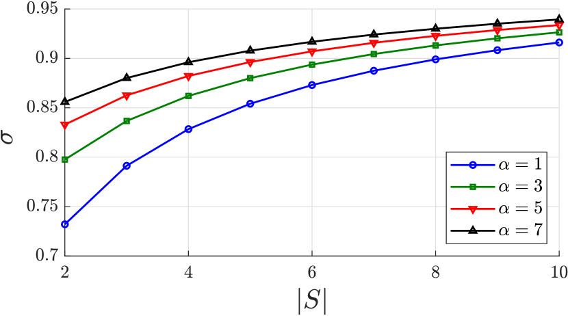
Figure 1: Subscription ratio at the equilibrium as a function of the number of NSTs for different values of $\alpha$.

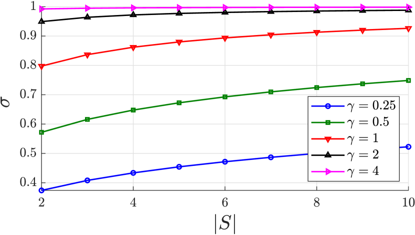
Figure 2: Subscription ratio at the equilibrium as a function of the number of NSTs for different values of $\gamma$.

In Figs. 1 and 2, the subscription ratio is represented as a function of the number of NSTs, for $\gamma=1$ and different values of $\alpha$ (Fig. 1) and for $\alpha=3$ and different values of $\gamma$ (Fig. 2). In all cases, as the number of NSTs increases, the subscription ratio increases, because $|\mathcal{S}|^{1-\beta}$ increases with $|\mathcal{S}|$ (note that $1-\beta>0$). This can be interpreted as that an increase in the diversity of the service offering increases the subscription ratio. Fig. 1 also shows that the subscription ratio increases with the user sensitivity. Fig. 2 also shows, in accordance with Proposition 2, that the greater the normalized capacity, the greater the subscription ratio. For $\gamma=4$, the subscription ratio is close to 1, which means that if the normalized capacity is high enough, the result is practically the same as for $r_{0}^{(r)}=0$ in all cells.

We now investigate how the asymmetry between the NSTs in terms of share affects the results. For this, we illustrate a scenario with 4 NSTs and $\alpha=3$, and show the results obtained as a function of the share of one of them.

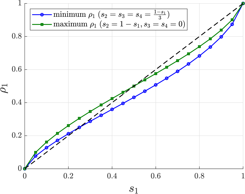
Figure 3: Maximum and minimum NST 1’s fraction of subscribers at the equilibrium as a function of its share.

Fig. 3 shows NST 1’s fraction of subscribers at the equilibrium as a function of its share in two different situations: one in which the remaining share is shared equally between the rest of NSTs ($s_{2}=s_{3}=s_{4}=(1-s_{1})/3$) and another one in which one NST keeps all the remaining share ($s_{2}=1-s_{1},\;s_{3}=s_{4}=0$). From (25), it is easy to show that the second situation (the one in which the remaining share is distributed as unequally as possible) is the most favorable for NST 1; thus, the corresponding curve represents the maximum fraction of subscribers that NST 1 can obtain. It can also be checked that the first situation, in which the remaining share is distributed equally, is the most unfavorable for NST 1, and now the curve represents the minimum fraction of subscribers. For any other distribution of the remaining share, the curve would run between these two bounds.

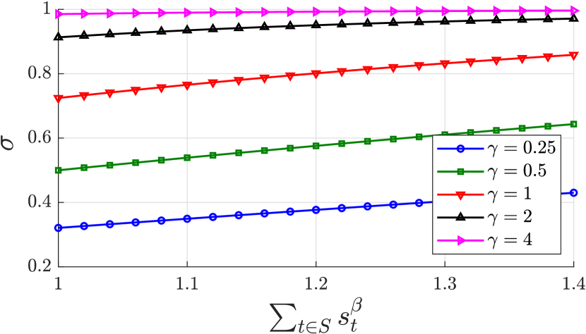
Figure 4: Subscription ratio at the equilibrium as a function of the term $\sum_{t\in S}s_{t}^{\beta}$ (share equality) for different values of $\gamma$.

Fig. 4 shows the subscription ratio as a function of the factor $\sum_{t\in\mathcal{S}}s_{t}^{\beta}$ for several values of $\gamma$. This factor depends on the degree of share equality and, together with $\gamma^{\beta}$, determines the result of (23). The figure shows that the higher the normalized capacity and the share equality, the higher the subscription ratio (Proposition 2). Also, according to Proposition 5, the maximum values of $\sigma$ correspond to $s_{i}=1/4$, when all shares are equal, and the minimum values are when a single NST takes all the share ($s_{1}=1,\;s_{2}=s_{3}=s_{4}=0$).

IV-B Heterogeneous cells

When cells are heterogeneous the proposed solution does not provide the exact equilibrium, but here we show that it provides an accurate approximation. We denote by $\tilde{w}_{i}^{(r)}$, $\tilde{\rho}_{i}$ and $\tilde{\sigma}^{(r)}$, the weights, fractions of subscribers and subscription ratios at the equilibrium, respectively, computed from the proposed solution, and keep the original names ($w_{i}^{(r)}$, $\rho_{i}^{(r)}$ and $\sigma^{(r)}$) for the results obtained with ABRD. Note that, although NST $i$’s fraction of subscribers obtained with the proposed solution ($\tilde{\rho}_{i}$) is the same for all cells, the one obtained with ABRD ($\rho_{i}^{(r)}$) is not. Besides, neither of the two subscription ratios ($\sigma^{(r)}$ or $\tilde{\sigma}^{(r)}$) is the same for all cells.

The plots in Figs. 5–7, correspond to a scenario with 4 NSTs, 5 cells and $\alpha=3$. NST 1’s share ranges from $0$ to $1$ and the remaining share is equally distributed between the rest of NSTs. The numbers of users are $(n^{(1)},\dots,n^{(5)})=(100,200,300,400,500)$, and the values of $c^{(r)}$ and $r_{0}^{(r)}$ have been chosen so that $(\gamma^{(1)},\dots,\gamma^{(5)})=(0.25,0.5,1,2,4)$. The marks represent the values obtained with ABRD, while the dashed lines represent the results of the proposed solution.

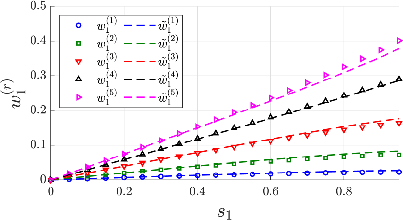
Figure 5: NST 1’s weights at the equilibrium as a function of NST 1’s share, compared with the proposed solution.

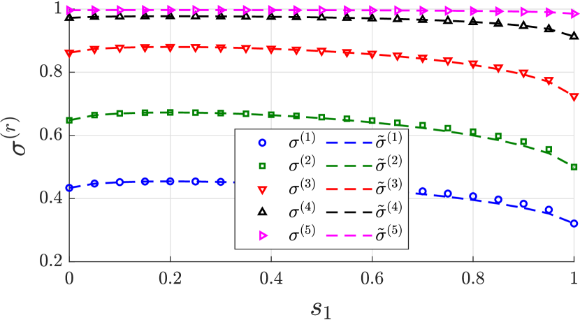
Figure 6: Subscription ratios in each cell at the equilibrium as a function of NST 1’s share, compared with the proposed solution.

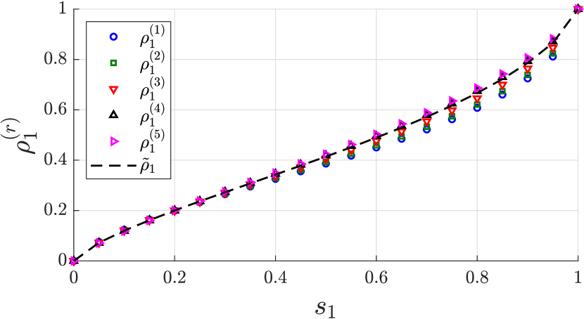
Figure 7: NST 1’s fractions of subscribers in each cell at the equilibrium as a function of NST 1’s share, compared with the proposed solution.

As seen in Figs. 5, NST 1’s weights obtained with ABRD are very close to the proposed solution. In the cells with lower $\gamma^{(r)}$ (cells 1, 2 and 3), they are slightly below the proposed solution, while in the cells with higher $\gamma^{(r)}$ (cells 4 and 5) they are slightly above. The subscription ratios in each cell are represented in Fig. 6, where the values obtained with both methods can hardly be distinguished from each other. Finally, in Fig. 7 it can be seen that NST 1’s fractions of subscribers are almost the same at the all cells, and that they are very close to the result of the proposed solution, which in fact is the same for all cells. Just like with the weights, the fractions of subscribers obtained with ABRD are slightly lower than those of the proposed solution in the cells with lower $\gamma^{(r)}$, and slightly higher in the cells with higher $\gamma^{(r)}$.

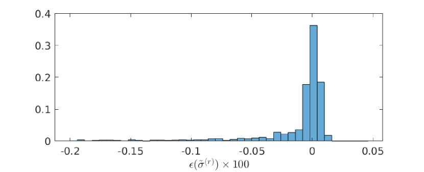
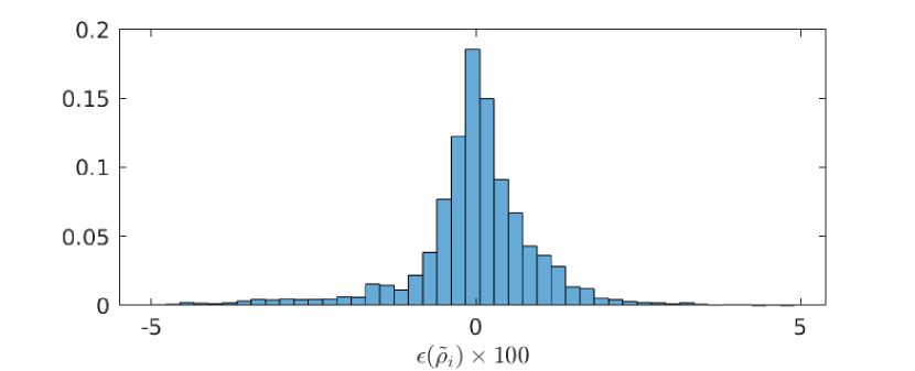
Figure 8: Histograms of the relative deviation (in percentage) of the subscription ratios and fractions of subscribers with the proposed solution.

These results suggest that the proposed solution provides a very good approximation of the equilibrium in a general case. In order to ensure the validity of this approach for a wide range of the system parameters, we have computed the deviation of the approximation for a diversity of types of scenario, each one with different numbers of NSTs, numbers of cells, values of $\alpha$ and ranges of $\gamma^{(r)}$. For each type of scenario, we have evaluated $1000$ scenarios both with the proposed solution and with ABRD. At each scenario, each $\gamma^{(r)},\;r\in\mathcal{B}$, has been generated randomly with uniform distribution in the range $[\gamma_{\min},\gamma_{\max}]$, and the shares have been generated as an equiprobable random vector in the $(|\mathcal{S}|-1)$-simplex $\{(s_{1}\dots s_{|\mathcal{S}|})\in\mathcal{R}^{|\mathcal{S}|}\mid\sum_{i\in\mathcal{S}}s_{i}=1,\;s_{i}\geq 0.1\}$. Relative deviations of the subscription ratio, $\epsilon(\tilde{\rho}_{i})$, and of the fraction of subscribers, $\epsilon(\tilde{\sigma}^{(r)})$, have been registered for all cases. They are calculated as: $\epsilon(\tilde{\rho}_{i})=(\tilde{\rho}_{i}-\rho_{i}^{(r)})/\rho_{i}^{(r)}$ and $\epsilon(\tilde{\sigma}^{(r)})=(\tilde{\sigma}^{(r)}-\sigma^{(r)})/\sigma^{(r)}$.

One of these types of scenario, the one with $4$ NSTs, $20$ cells, $\alpha=3$ and $\gamma^{(r)}\in[0.25,4]$ is illustrated in the histograms of Fig. 8, where the relative deviations are expressed as percentages. We see that the values of the relative deviation of the fraction of subscribers are distributed almost symmetrically around 0 and most values are below $1\,\%$. The relative deviation of the subscription ratio is even smaller (most values are below $0.1\,\%$) and that negative values are more frequent, which suggests that the proposed solution tends to provide an underestimate.

Table I: Percentiles of the module of $\epsilon(\tilde{\rho}_{i})$ and $\epsilon(\tilde{\sigma}^{(r)})$ (in percentage)

				$|\epsilon(\tilde{\rho}_{i})|\times 100$			$|\epsilon(\tilde{\sigma}^{(r)})|\times 100$
$S$	$R$	$\alpha$	$[\gamma_{\min},\gamma_{\max}$]	$P_{90}$	$P_{95}$		$P_{90}$	$P_{95}$
$2$	$10$	$1$	$[0.25,4]$	$1.5$	$2.0$		$0.112$	$0.193$
		$3$		$2.7$	$3.8$		$0.112$	$0.240$
		$5$		$2.6$	$4.0$		$0.093$	$0.208$
		$7$		$2.1$	$4.0$		$0.051$	$0.151$
$2$	$20$	$1$	$[0.25,4]$	$1.9$	$2.7$		$0.141$	$0.311$
		$3$		$2.9$	$4.1$		$0.138$	$0.284$
		$5$		$2.5$	$3.8$		$0.071$	$0.174$
		$7$		$2.0$	$2.9$		$0.042$	$0.106$
$4$	$20$	$1$	$[0.25,4]$	$0.6$	$0.8$		$0.026$	$0.050$
		$3$		$1.5$	$2.2$		$0.061$	$0.131$
		$5$		$1.2$	$1.8$		$0.033$	$0.064$
		$7$		$1.3$	$2.1$		$0.036$	$0.071$
$2$	$10$	$3$	$[0.25,0.5]$	$0.4$	$0.6$		$0.039$	$0.053$
			$[0,1]$	$0.7$	$1.2$		$0.064$	$0.082$
			$[1,2]$	$1.0$	$1.5$		$0.038$	$0.054$
			$[2,4]$	$0.6$	$0.9$		$0.007$	$0.011$
$2$	$20$	$3$	$[0.25,0.5]$	$0.4$	$0.6$		$0.039$	$0.055$
			$[0,1]$	$1.1$	$1.6$		$0.082$	$0.104$
			$[1,2]$	$1.1$	$1.9$		$0.050$	$0.075$
			$[2,4]$	$0.6$	$0.9$		$0.007$	$0.012$
$4$	$20$	$3$	$[0.25,0.5]$	$0.4$	$0.5$		$0.028$	$0.036$
			$[0,1]$	$0.7$	$0.9$		$0.038$	$0.051$
			$[1,2]$	$0.7$	$0.9$		$0.015$	$0.023$
			$[2,4]$	$0.3$	$0.3$		$0.005$	$0.005$

Table I shows the 90th and 95th percentiles of the module of $\epsilon(\tilde{\rho}_{i})$ and $\epsilon(\tilde{\sigma}^{(r)})$ for a wide range of scenarios. It is observed that the deviations are slightly higher when $\gamma^{(r)}$ values are smaller (in the range $[0.25,0.5]$). But even in the worst case, the 95th percentile of $|\epsilon(\tilde{\rho}_{i})|$ is below $4.2\,\%$ and the 95th percentile of $|\epsilon(\tilde{\sigma}^{(r)})|$ is below $0.32\,\%$.

V Conclusions

In this work, a business model is proposed and analyzed where the NSTs provide mobile communications services to final users and provision themselves with resources from an InP by means of network slicing mechanisms. Each NST splits its share of the resources by choosing a weight for each cell. Weights determine the proportion of resources that each NST obtain in each cell, which in turn determines the service that it can offer to users and therefore the number of users subscribed. Each NST chooses its weights strategically in order to maximize its number of subscribers.

We propose a solution for the Nash equilibrium in which every NST chooses, for each cell, a weight equal to the product of its share by the ratio between the total number of subscribers in the cell and the total number of subscribers in the network. This solution allows us to argue that network slicing provides an attractive flexibility in the allocation of resources without the need to enforce or control a policy through the InP.

For this solution, all the values at the equilibrium can be easily computed through the expressions provided. The proposed solution has the following properties:

• It provides the exact values at the equilibrium if the cells are homogeneous in terms of normalized capacity. In this case, the subscription ratio is the same in all cells.

• Otherwise, if the cells are heterogeneous, it provides an accurate approximation of the equilibrium.

• In each cell, the subscription ratio increases with the normalized capacity, and depends on the share distribution, being maximum when all shares are equal.

• Each NST obtains a fraction of subscribers which is the same in all cells. It depends only on its share, the user sensitivity and the share distribution, and is minimum when the shares of all the other NSTs are equal.

Let $f(x)=x-a(1-x)^{1-\beta}$, with $a>0$ and $\beta<1$.

Lemma 1

The function $f(x)$ has one, and only one, root in $(0,1)$.

Proof of Proposition 1

When $r_{0}^{(j)}>0$, we can rewrite (8) as

$$\left(\frac{\omega^{(j)}_{i}}{n^{(j)}_{i}}\right)^{\alpha}=\frac{n^{(j)}_{i}}{n^{(j)}}\left(\sum_{t\in\mathcal{S}}\left(\frac{\omega^{(j)}_{t}}{n^{(j)}_{t}}\right)^{\alpha}+\left(\frac{\sum_{t\in\mathcal{S}}\omega^{(j)}_{t}}{n^{(j)}\gamma^{(j)}}\right)^{\alpha}\right),\\ i\in\mathcal{S},\quad j\in\mathcal{B}.$$ (45)

Now, adding (45) over all $i\in\mathcal{S}$ yields

$$\sum_{t\in\mathcal{S}}\left(\frac{\omega^{(j)}_{t}}{n^{(j)}_{t}}\right)^{\alpha}=\sigma^{(j)}\sum_{t\in\mathcal{S}}\left(\frac{\omega^{(j)}_{t}}{n^{(j)}_{t}}\right)^{\alpha}+\sigma^{(j)}\left(\frac{\sum_{t\in\mathcal{S}}\omega^{(j)}_{t}}{n^{(j)}\gamma^{(j)}}\right)^{\alpha},\\ j\in\mathcal{B},$$ (46)

which can be rewritten as

$$\sum_{t\in\mathcal{S}}\left(\frac{\omega^{(j)}_{t}}{n^{(j)}_{t}}\right)^{\alpha}=\frac{\sigma^{(j)}}{1-\sigma^{(j)}}\left(\frac{\sum_{t\in\mathcal{S}}\omega^{(j)}_{t}}{n^{(j)}\gamma^{(j)}}\right)^{\alpha},\quad j\in\mathcal{B}.$$ (47)

Substituting (47) into (45) and solving for $n^{(j)}_{i}$ yields

$$\frac{n^{(j)}_{i}}{n^{(j)}}=\left(1-\sigma^{(j)}\right)^{1-\beta}\left(\gamma^{(j)}\right)^{\beta}\frac{\left(\omega^{(j)}_{i}\right)^{\beta}}{\left(\sum_{t\in\mathcal{S}}\omega^{(j)}_{t}\right)^{\beta}},\\ i\in\mathcal{S},\quad j\in\mathcal{B},$$ (48)

where $\beta=\alpha/(\alpha+1)<1$.

Finally, adding (48) over all $i\in\mathcal{S}$, we obtain

$$\sigma^{(j)}-\left(\gamma^{(j)}\right)^{\beta}\frac{\sum_{t\in\mathcal{S}}\left(\omega^{(j)}_{t}\right)^{\beta}}{\left(\sum_{t\in\mathcal{S}}\omega^{(j)}_{t}\right)^{\beta}}\left(1-\sigma^{(j)}\right)^{1-\beta}=0,\qquad j\in\mathcal{B}.$$ (49)

The application of Lemma 1 guarantees that (49) has a unique solution in $(0,1)$.

In the case $r_{0}^{(j)}=0$, we can rewrite (8) as

$$\left(\frac{\omega^{(j)}_{i}}{n^{(j)}_{i}}\right)^{\alpha}=\frac{n^{(j)}_{i}}{n^{(j)}}\sum_{t\in\mathcal{S}}\left(\frac{\omega^{(j)}_{t}}{n^{(j)}_{t}}\right)^{\alpha},\qquad i\in\mathcal{S},\quad j\in\mathcal{B}.$$ (50)

Adding this equality over all $i\in\mathcal{S}$ immediately leads to $\sigma^{(j)}=1$.

Luis Guijarro Luis Guijarro received the M.Eng. and Ph.D. degrees in telecommunications from the Universitat Politècnica de València (UPV), Valencia, Spain. He is currently an Associate Professor in telecommunications policy with the Department of Communications, UPV. He has authored or coauthored the book Electronic Communications Policy of the European Union (UPV, 2010). He researched in traffic management in ATM networks and in e-Government. His current research interest includes economic modeling of telecommunication service provision. He has contributed in the areas of peer-to-peer interconnection, cognitive radio networks, search engine neutrality, wireless sensor networks, and 5G.

References

- [1] NGMN Alliance, “Description of network slicing concept,” Next Generation Mobile Networks, White paper, 2016.
- [2] M. Jiang, M. Condoluci, and T. Mahmoodi, “Network slicing management & prioritization in 5G mobile systems,” in European Wireless Conference 2016, EW 2016, 2016, pp. 197–202.
- [3] K. Samdanis, X. Costa-Perez, and V. Sciancalepore, “From network sharing to multi-tenancy: The 5G network slice broker,” IEEE Communications Magazine, vol. 54, no. 7, pp. 32–39, 2016.
- [4] NGMN Alliance, “5G white paper,” Next Generation Mobile Networks, White paper, 2015.
- [5] D. Niyato and E. Hossain, “Competitive pricing for spectrum sharing in cognitive radio networks: Dynamic game, inefficiency of Nash equilibrium, and collusion,” IEEE Journal on Selected Areas in Communications, vol. 26, no. 1, pp. 192–202, 2008.
- [6] L. Guijarro, V. Pla, J. R. Vidal, and M. Naldi, “Game theoretical analysis of service provision for the internet of things based on sensor virtualization,” IEEE Journal on Selected Areas in Communications, vol. 35, no. 3, pp. 691–706, 2017.
- [7] ——, “Competition in data-based service provision: Nash equilibrium characterization,” Future Generation Comp. Syst., vol. 96, pp. 35–50, 2019.
- [8] S. Brânzei, Y. Chen, X. Deng, A. Filos-Ratsikas, S. K. S. Frederiksen, and J. Zhang, “The fisher market game: equilibrium and welfare,” in Twenty-Eighth AAAI Conference on Artificial Intelligence, 2014.
- [9] M. Feldman, K. Lai, and L. Zhang, “The proportional-share allocation market for computational resources,” IEEE Transactions on Parallel and Distributed Systems, vol. 20, no. 8, pp. 1075–1088, 2009.
- [10] P. Caballero, A. Banchs, G. de Veciana, and X. Costa-Pérez, “Network slicing games: Enabling customization in multi-tenant networks,” in INFOCOM 2017-IEEE Conference on Computer Communications. IEEE, 2017, pp. 1–9.
- [11] S. O. Oladejo and O. E. Falowo, “5G network slicing: A multi-tenancy scenario,” in Wireless Summit (GWS), 2017 Global. IEEE, 2017, pp. 88–92.
- [12] M. E. Ben-Akiva and S. R. Lerman, Discrete choice analysis: theory and application to travel demand. MIT press, 1985, vol. 9.
- [13] P. Maillé and B. Tuffin, Telecommunication network economics: from theory to applications. Cambridge University Press, 2014.
- [14] P. Reichl, B. Tuffin, and R. Schatz, “Logarithmic laws in service quality perception: where microeconomics meets psychophysics and quality of experience,” Telecommunication Systems, pp. 1–14, 2011.
- [15] K. E. Train, Discrete choice methods with simulation. Cambridge university press, 2009.
- [16] “Modified cuckoo search: A new gradient free optimisation algorithm,” Chaos, Solitons & Fractals, vol. 44, no. 9, pp. 710 – 718, 2011.