The confining color field in SU(3) gauge theory

Abstract

We extend a previous numerical study of SU(3) Yang-Mills theory in which we measured the spatial distribution of all components of the color fields surrounding a static quark-antiquark pair for a wide range of quark-antiquark separations, and provided evidence that the simulated gauge invariant chromoelectric field can be separated into a Coulomb-like ’perturbative’ field and a ’non-perturbative’ field, identified as the confining part of the SU(3) flux tube field.

In this paper we hypothesize that the fluctuating color fields not measured in our simulations do not contribute to the string tension. Under this assumption the string tension is determined by the color fields we measure, which form a tensor $F_{\mu\nu}$ pointing in a single direction in color space. We call this the Maxwell mechanism of confinement.

We provide an additional procedure to isolate the non-perturbative (confining) field. We then extract the string tension from a stress energy-momentum tensor $T_{\mu\nu}$ having the Maxwell form, constructed from the non-perturbative part of the tensor $F_{\mu\nu}$ obtained from our simulations.

To test our hypothesis we calculate the string tension from our simulations of the color fields for ten values of the quark-antiquark separation ranging from 0.37 fm to 1.2 fm. We also calculate the spatial distributions of the energy-momentum tensor $T_{\mu\nu}$ surrounding static quarks for this range of separations, and we compare these distributions with those obtained from direct simulations of the energy-momentum tensor in SU(3) Yang-Mills theory.

1 Introduction

Quantum chromodynamics (QCD) is universally accepted as the theory of strong interactions. Nobody doubts that the well established phenomenon of confinement of quarks and gluons inside hadrons is encoded into the QCD Lagrangian. Yet, our current understanding does not go beyond that provided by a number of models of the QCD vacuum (for a review, see Refs. greensite2011introduction ; Diakonov:2009jq ). In particular, a theoretical a priori explanation of the so called area law in large size Wilson loops, which is closely related to a linear confining potential between a static quark and antiquark at large mutual distances, is still missing.

In such a challenging situation, first-principle Monte Carlo simulations of QCD on a space-time lattice represent an indispensable tool not only for checking (or ruling out) models of confinement, but also for providing new numerical “phenomenology” and possibly stimulating original insights into the mechanism of confinement.

Numerical simulations have established that there is a linear confining potential between a static quark and antiquark for distances equal to or larger than about 0.5 fm. This linear regime extends to infinite distances in SU(3) pure gauge theory, and, in the presence of dynamical quarks to distances of about 1.4 fm, where string breaking should take place Philipsen:1998de ; Kratochvila:2002vm ; Bali:2005fu . The long-distance linear quark-antiquark potential is naturally associated with a tube-like structure (“flux tube”) of the chromoelectric field in the longitudinal direction, i.e. along the line connecting the static quark and antiquark Bander:1980mu ; Greensite:2003bk ; Ripka:2005cr ; Simonov:2018cbk .

A wealth of numerical evidence of flux tubes has accumulated in SU(2) and SU(3) Yang-Mills theories Fukugita:1983du ; Kiskis:1984ru ; Flower:1985gs ; Wosiek:1987kx ; DiGiacomo:1989yp ; DiGiacomo:1990hc ; Cea:1992sd ; Matsubara:1993nq ; Cea:1994ed ; Cea:1995zt ; Bali:1994de ; Green:1996be ; Skala:1996ar ; Haymaker:2005py ; D'Alessandro:2006ug ; Cardaci:2010tb ; Cea:2012qw ; Cea:2013oba ; Cea:2014uja ; Cea:2014hma ; Cardoso:2013lla ; Caselle:2014eka ; Cea:2015wjd ; Cea:2017ocq ; Shuryak:2018ytg ; Bonati:2018uwh ; Shibata:2019bke . Most of these studies concentrated on the shape of the chromoelectric field on the transverse plane at the midpoint of the line connecting the static quark and antiquark, given that the other two components of the chromoelectric field and all the three components of the chromomagnetic field are suppressed in that plane.

Recent times have witnessed an increasing numerical effort toward a more comprehensive numerical description of the color field around static sources, via the measurement of all components of both chromoelectric and chromomagnetic fields on all transverse planes passing through the line between the quarks Baker:2018mhw ; of the spatial distribution of the stress energy momentum tensor Yanagihara:2018qqg ; Yanagihara:2019foh ; and the flux densities for hybrid static potentials Bikudo:2018 ; Mueller:2019mkh . A more complete numerical description of the color field around the sources brings improved visualization, enabling us to grasp features otherwise less visible.

In the numerical study Baker:2018mhw we simulated the spatial distribution in three dimensions of all components of the chromoelectric and chromomagnetic fields generated by a static quark-antiquark pair in pure SU(3) lattice gauge theory. We found that, although the components of the simulated chromoelectric field transverse to the line connecting the pair are smaller than the simulated longitudinal chromoelectric field, these transverse components are large enough to be fit to a Coulomb-like ‘perturbative’ field produced by two static sources parameterized by effective charges $\pm Q$ of the sources (see Eq. (5) below).

The longitudinal component of this Coulomb-like ‘perturbative’ field accounts for a fraction of the simulated longitudinal chromoelectric field. We then identified the remaining longitudinal chromoelectric field as the confining ‘non-perturbative’ part of the simulated SU(3) flux tube field.

It is this non-perturbative part of the simulated field which contributes to the coefficient of the linear term in the heavy quark potential, the string tension.

In this paper we extend our simulations to a wider range of quark-antiquark separations. We extract the string tension from these simulations and compare our analysis with the results of recent simulations Yanagihara:2018qqg of the energy-momentum tensor in SU(3) Yang-Mills theory.

We present a new procedure (the curl method) to extract a perturbative Coulomb field $\vec{E}^{\rm C}$ from the transverse components of the numerically simulated chromoelectric field. We avoid the use of a fitting function, directly imposing the condition that $\vec{E}^{\rm C}$ is irrotational (see Eq. (6) below). This provides a second method for implementing the underlying idea of our previous paper; that is, the chromoelectric field generated by a quark-antiquark pair can be separated into perturbative and non-perturbative components by a direct analysis of lattice data on the color field distributions generated by the pair.

As noted in Baker:2018mhw , we can extract the value of the string tension from the non-perturbative field by utilizing the fact that the value of the chromoelectric field at the position of a quark is the force on the quark Brambilla:2000gk . However, the Coulomb-like field (Eq. (5)) does not give a good description of the transverse components of the chromoelectric field at distances closer than approximately two lattice steps from the sources Baker:2018mhw , so that we must use the curl method to isolate the confining field in order to extract the string tension directly as the force.

The color fields $F_{\mu\nu}$ we measure, defined by the gauge invariant correlation function $\rho^{\rm conn}_{W,\mu\nu}$ (see Eqs. (1) and (2), below), point in a single direction in color space, parallel to the direction of the ‘source’ Wilson loop. In this paper we construct a stress energy -momentum tensor $T_{\mu\nu}$ having the Maxwell form from the ‘measured’ flux tube field tensor $F_{\mu\nu}$, and extract the string tension (see A). This leads to a picture of a confining flux tube permeated with lines of force of a gauge invariant field tensor $F_{\mu\nu}$ carrying color charge along a single direction.

The ‘Maxwell’ energy-momentum tensor $T_{\mu\nu}$ does not account for the contribution to the quark-antiquark force from the fluctuating color fields not measured in our simulations. On the other hand, the complete Yang-Mills energy momentum tensor $T^{\rm YM}_{\mu\nu}$ simulated in Ref. Yanagihara:2018qqg includes these fluctuating contributions, so that comparison of $T^{\rm YM}_{\mu\nu}$ with the ’Maxwell’ energy-momentum tensor $T_{\mu\nu}$ constructed from the chromoelectric and chromomagnetic fields measured in our simulations provides a measure of the fluctuating contributions to the stress tensor.

We noted in our previous paper that the Coulomb-like ‘perturbative’ field (Eq. (5)) generated a stronger long distance Coulomb force between the heavy quarks than the Coulomb force measured in lattice simulations of the heavy quark potential Necco:2001xg ; Kaczmarek:2005ui ; Karbstein:2018mzo indicating the importance of fluctuations for the Coulomb contribution. In this paper we reexamine this issue.

The paper is organized as follows: in Section 2 we present the theoretical background and the lattice setup. In Section 3 we show some results on the spatial distribution of the color field around the two static sources and review the procedure to extract its non-perturbative part by subtraction of the Coulomb-like perturbative part identified by a fit of the transverse components of the chromoelectric field; in Section 4 we describe the new curl method to isolate the non-perturbative part; in Section 5 we show how to determine the string tension and other fundamental parameters describing the (non-perturbative) flux tube; finally, in Section 6 we discuss our results and give some ideas for future work.

2 Theoretical background and lattice setup

The lattice operator whose vacuum expectation value gives us access to the components of the color field generated by a static $q\bar{q}$ pair is the following connected correlator DiGiacomo:1989yp ; DiGiacomo:1990hc ; Kuzmenko:2000bq ; DiGiacomo:2000va :

$$\rho_{W,\,\mu\nu}^{\rm conn}=\frac{\left\langle{\rm tr}\left(WLU_{P}L^{\dagger}\right)\right\rangle}{\left\langle{\rm tr}(W)\right\rangle}-\frac{1}{N}\,\frac{\left\langle{\rm tr}(U_{P}){\rm tr}(W)\right\rangle}{\left\langle{\rm tr}(W)\right\rangle}\;.$$ (1)

Here $U_{P}=U_{\mu\nu}(x)$ is the plaquette in the $(\mu,\nu)$ plane, connected to the Wilson loop $W$ by a Schwinger line $L$, and $N$ is the number of colors (see Fig. 1).

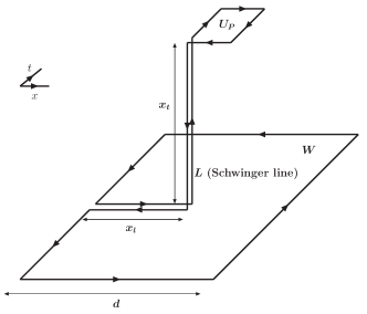
(a)                       

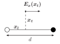
Figure 1:  1(a) The connected correlator given in Eq. (1) between the plaquette $U_{P}$ and the Wilson loop (subtraction in $\rho_{W,\,\mu\nu}^{\rm conn}$ not explicitly drawn).  1 The longitudinal chromoelectric field $E_{x}(x_{t})$ relative to the position of the static sources (represented by the white and black circles), for a given value of the transverse distance $x_{t}$.

The correlation function defined in Eq. (1) measures the field strength $F_{\mu\nu}$, since in the naive continuum limit DiGiacomo:1990hc

$$\rho_{W,\,\mu\nu}^{\rm conn}\stackrel{{\scriptstyle a\rightarrow 0}}{{\longrightarrow}}a^{2}g\left[\left\langle F_{\mu\nu}\right\rangle_{q\bar{q}}-\left\langle F_{\mu\nu}\right\rangle_{0}\right]\;,$$ (2)

where $\langle\quad\rangle_{q\bar{q}}$ denotes the average in the presence of a static $q\bar{q}$ pair, and $\langle\quad\rangle_{0}$ is the vacuum average. This relation is a necessary consequence of the gauge-invariance of the operator defined in Eq. (1) and of its linear dependence on the color field in the continuum limit (see Ref. Cea:2015wjd ).

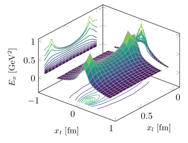
(a) $E_{x}(x_{t},x_{l})$

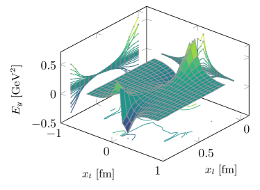
(b) $E_{y}(x_{t},x_{l})$

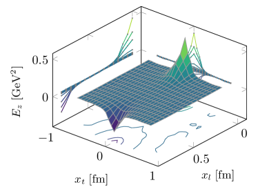
(c) $E_{z}(x_{t},x_{l})$

Figure 2: Surface and contour plots for the three components of the chromoelectric field at $\beta=6.370$ and $d=0.85$ fm. All plotted quantities are in physical units.

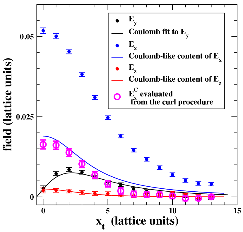
Figure 3: The three components of the chromoelectric field measured at $\beta=6.240$, $d=16a=1.02\ \mathrm{fm}$, for $x_{l}=4a$ and the three components of the perturbative Coulomb field, obtained from fitting the transverse $E_{y}$ field component to the form (5).

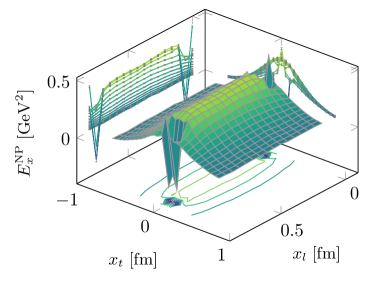
(a) $E_{x}^{\rm NP}(x_{t},x_{l})$

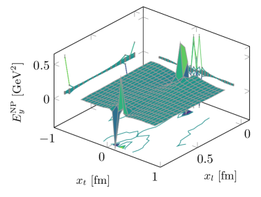
(b) $E_{y}^{\rm NP}(x_{t},x_{l})$

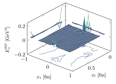
(c) $E_{z}^{\rm NP}(x_{t},x_{l})$

Figure 4: Surface and contour plots for the three components of the non-perturbative chromoelectric field, $\vec{E}^{\rm NP}\equiv\vec{E}-\vec{E}^{\rm C}$, at $\beta=6.370$ and $d=0.85~{}$ fm. All plotted quantities are in physical units.

The lattice definition of the quark-antiquark field-strength tensor $F_{\mu\nu}$ is then obtained by equating the two sides of Eq. (2) for finite lattice spacing. In the particular case when the Wilson loop $W$ lies in the plane with $\hat{\mu}=\hat{4}$ and $\hat{\nu}=\hat{1}$ (see Fig. 1(a)) and the plaquette $U_{P}$ is placed in the planes $\hat{4}\hat{1}$, $\hat{4}\hat{2}$, $\hat{4}\hat{3}$, $\hat{2}\hat{3}$, $\hat{3}\hat{1}$, $\hat{1}\hat{2}$, we get, respectively, the color field components $E_{x}$, $E_{y}$, $E_{z}$, $B_{x}$, $B_{y}$, $B_{z}$, at the spatial point corresponding to the position of the center of the plaquette, up to a sign depending on the orientation of the plaquette. Because of the symmetry (Fig. 1), the color fields take on the same values at spatial points connected by rotations around the axis on which the sources are located (the $\hat{1}$- or $x$-axis in the given example) .

As far as the color structure of the field $F_{\mu\nu}$ is concerned, we note that the source of $F_{\mu\nu}$ is the Wilson loop connected to the plaquette in Fig. 1. The role of the Schwinger lines entering Eq. (1) is to realize the color parallel transport between the source loop and the “probe” plaquette. The Wilson loop defines a direction in color space. The color field $\vec{E}$ that we measure in Eq. (2) points in that direction in the color space, i.e. in the color direction of the source.

There are fluctuations of the color fields in the other color directions. We assume that these fluctuating color fields do not contribute to the string tension, so that the flux tube can be described as lines of force of the simulated field $\vec{E}$.

The simulated flux tube field $\vec{E}$ carries color electric charge and color magnetic current along a single direction in color space. The divergence of $\vec{E}$ is equal to the color electric charge density $\rho_{\rm el}(\vec{x})$ and the curl of $\vec{E}$ is equal to the color magnetic current density $\vec{J}_{\rm M}(\vec{x})$. The confining force is calculated from the divergence of a stress tensor $T_{\mu\nu}$ having the Maxwell form Eq. (13) .

The operator in Eq. (1) undergoes a non-trivial renormalization, which depends on $x_{t}$, as discussed in a recent work Battelli:2019lkz . The procedure outlined in that paper to properly take into account these renormalization effects is prohibitively demanding from the computational point of view for Wilson loops and Schwinger lines with linear dimension of the order of 1 fm, where the interesting physics is expected to take place. For this reason, we adopt here the traditional approach to perform smearing on the Monte Carlo ensemble configurations before taking measurements (see below for details). As shown in the Appendix A of our previous paper Baker:2018mhw , smearing behaves as an effective renormalization, effectively pushing the system towards the continuum, where renormalization effects become negligible. The a posteriori validation of the smearing procedure is provided by the observation of continuum scaling: as carefully checked in Ref. Cea:2017ocq , fields obtained in the same physical setup, but at different values of the coupling, are in perfect agreement in the range of parameters used in the present work.

We performed all simulations in SU(3) pure gauge theory, with the standard Wilson action as the lattice discretization. A summary of the runs performed is given in Table 1. The error analysis was performed by the jackknife method over bins at different blocking levels.

Table 1: Summary of the runs performed in the SU(3) pure gauge theory (measurements are taken every 100 upgrades of the lattice configuration).

$\beta$	lattice	$a$[fm]	$d$ [lattice]	$d$ [fm]	statistics	smearing steps, $N_{\rm APE}$
6.47466	$36^{4}$	0.047	8	0.37	12900	100
6.333	$48^{4}$	0.056	8	0.45	180	80
6.240	$48^{4}$	0.064	8	0.51	1300	60
6.500	$48^{4}$	0.045	12	0.54	3900	100
6.539	$48^{4}$	0.043	16	0.69	6300	100
6.370	$48^{4}$	0.053	16	0.85	5300	100
6.299	$48^{4}$	0.059	16	0.94	10700	100
6.240	$48^{4}$	0.064	16	1.02	21000	100
6.218	$48^{4}$	0.066	16	1.06	32000	100
6.136	$48^{4}$	0.075	16	1.19	84000	120

We set the physical scale for the lattice spacing according to Ref. Necco:2001xg :

$$a(\beta)=r_{0}\!\times\!\exp\left[c_{0}+c_{1}(\beta\!-\!6)+c_{2}(\beta\!-\!6)^{2}+c_{3}(\beta\!-\!6)^{3}\right],$$

$$r_{0}=0.5\;{\rm fm},$$

$$c_{0}=-1.6804\,,c_{1}=-1.7331\,,$$

$$c_{2}=0.7849\,,c_{3}=-0.4428\,,$$ (3)

for all $\beta$ values in the range $5.7\leq\beta\leq 6.92$. In this scheme the value of the square root of the string tension $\sqrt{\sigma}\approx 0.465\,{\textrm{GeV}}$ (see Eq. (3.5) in Ref. Necco:2001xg ).

The correspondence between $\beta$ and the distance $d$ shown in Table 1 was obtained from this parameterization. Note that the distance in lattice units between quark and antiquark, corresponding to the spatial size of the Wilson loop in the connected correlator of Eq. (1), was varied in the range $d=8\,a$ to $d=16\,a$.

The connected correlator defined in Eq. (1) exhibits large fluctuations at the scale of the lattice spacing, which are responsible for a bad signal-to-noise ratio. To extract the physical information carried by fluctuations at the physical scale (and, therefore, at large distances in lattice units) we smoothed out configurations by a smearing procedure. Our setup consisted of (just) one step of HYP smearing Hasenfratz:2001hp on the temporal links, with smearing parameters $(\alpha_{1},\alpha_{2},\alpha_{3})=(1.0,0.5,0.5)$, and $N_{\rm APE}$ steps of APE smearing Falcioni1985624 on the spatial links, with smearing parameter $\alpha_{\rm APE}=0.25$.

3 Spatial distribution of the color fields

Using Monte Carlo evaluations of the expectation value of the operator $\rho_{W,\,\mu\nu}$ over smeared ensembles, we have determined the six components of the color fields on all two-dimensional planes transverse to the line joining the color sources allowed by the lattice discretization. These measurements were carried out for several values of the distance $d$ between the static sources, in the range 0.37 fm to 1.19 fm, at values of $\beta$ lying inside the continuum scaling region, as determined in Ref. Cea:2017ocq .

We found that the chromomagnetic field is everywhere much smaller than the longitudinal chromoelectric field and is compatible with zero within statistical errors (see, e.g., Fig. 3 of Ref. Baker:2018mhw ). As expected, the dominant component of the chromoelectric field is longitudinal, as is seen in Fig. 2, where we plot the components of the simulated chromoelectric field $\vec{E}$ at $\beta=6.370$ as functions of their longitudinal displacement from one of the quarks, $x_{l}$, and their transverse distance from the axis, $x_{t}$.

While the transverse components of the chromoelectric field are also smaller than the longitudinal component, they are larger than the statistical errors in a region wide enough that we can match them to the transverse components of an effective Coulomb-like field $\vec{E}^{\rm C}$ produced by two static sources. For points which are not very close to the quarks, this matching can be carried out with a single fitting parameter $Q$, the effective charge of static quark and antiquark sources determining $\vec{E}^{\rm C}$.

To the extent that we can fit the transverse components of the simulated field $\vec{E}$ to those of $\vec{E}^{\rm C}$ with an appropriate choice of $Q$, the non-perturbative difference $\vec{E}^{\rm NP}$ between the simulated chromoelectric field $\vec{E}$ and the effective Coulomb field $\vec{E}^{\rm C}$,

$$\vec{E}^{\rm NP}~{}\equiv~{}\vec{E}~{}-~{}\vec{E}^{\rm C}\;,$$ (4)

will be purely longitudinal. We then identify $\vec{E}^{\rm NP}$ as the confining field of the QCD flux tube.

To illustrate this idea, let us fix, for the sake of definiteness, $\beta=6.240$ and put the two sources at a distance $d=16a=1.02~{}$ fm. We then consider the plane, transverse to the longitudinal $x$-axis connecting the two sources, at a distance $x_{l}=4a$ from one of them, and evaluate the components $E_{x}$, $E_{y}$ and $E_{z}$ of the chromoelectric field in this transverse plane. The lattice determinations of $E_{y}$ on this plane can be fitted by the $y$-component of an effective Coulomb field

$$\vec{E}^{\rm C}(\vec{r})\;=\;Q\left(\frac{\vec{r}_{1}}{\max(r_{1},R_{0})^{3}}\;-\;\frac{\vec{r}_{2}}{\max(r_{2},R_{0})^{3}}\;\right)\;,$$ (5)

$$\vec{r}_{1}\equiv\vec{r}-\vec{r}_{Q}\;,\;\;\;\vec{r}_{2}\equiv\vec{r}-\vec{r}_{-Q}\;,$$

where $\vec{r}_{Q}$ and $\vec{r}_{-Q}$ are the positions of the two static color sources and $R_{0}$ is the effective radius of the color source, introduced to explain, at least partially, the decrease of the field close to the sources. This fit is shown in Fig. 3 – see black dots and black solid line. Using the values of the fit parameters $Q$ and $R_{0}$ obtained by the fit of $E_{y}$, one can construct $E_{z}^{\rm C}$ and $E_{x}^{\rm C}$ and compare them to lattice data. Furthermore, the Coulomb-like content of $E_{z}$ fully accounts for the $z$-component of the chromoelectric field (see red dots and red solid line in Fig. (3)), but $E_{x}^{\rm C}$ accounts for only a fraction of the longitudinal component of the chromoelectric field (see blue dots and blue solid line in Fig. (3)). This strongly suggests that the non-perturbative component of the chromoelectric field is almost completely oriented along the longitudinal direction. It can be isolated once the parameters of the Coulomb-like component are determined by a fit to the $y$- and/or $z$-components of the lattice determination of the chromoelectric field.

The procedure we have just illustrated in a specific case, can be carried out in a systematic manner. We observe that in making the fit we must take into account that the color fields are probed by a plaquette, so that the measured field value should be assigned to the center of the plaquette. This also means that the $z$-component of the field is probed at a distance of $1/2$ lattice spacing from the $x\,y$ plane, where the $z$-component of the Coulomb field $E_{z}^{\rm C}$ is non-zero and can be matched with the measured value $E_{z}$ for the same value of $Q$. For further details about the fitting procedure and the extraction of the fit parameters we refer to Appendix B of Ref. Baker:2018mhw .

In Table 2, we list the values of the effective charge $Q$ obtained from the lattice measurements of $E_{z}$ and $E_{y}$ at the values of $d$, the quark-antiquark separation, considered in this work.

Table 2: Values of the fit parameters $Q$ and $R_{0}$ extracted from Coulomb fits of the transverse components of the chromoelectric field and values of the longitudinal chromoelectric fields at $(d/2,0)$, the midpoint between the sources and transverse distance zero, for several values of distance $d$. $E_{x}(d/2,0)$ is the unsubtracted simulated field and $E_{x}^{\rm NP}(d/2,0)$ is the non-perturbative chromoelectric field. For comparison, in the last column the non-perturbative chromoelectric field ${E_{x}^{\rm NP}}_{\mathrm{curl}}(d/2,0)$ obtained using the irrotational property of the perturbative field (see section 4) is given. For the parameters of the Coulomb fit we quote, along with the statistical error, a systematic uncertainty that accounts for the variability in the values of the fit parameters extracted from all acceptable fits to $E_{y}$ and $E_{z}$ at different $x_{l}$ values (for more details, see Appendix B of Ref. Baker:2018mhw ). As the distance between the sources is made smaller and smaller the quality of the Coulomb fits deteriorates and $Q$ and $R_{0}$ cannot be reliably extracted for $d\leq 0.51$ fm.

$\beta$	$d$ [fm]	$Q$	$R_{0}$ [fm]	$E_{x}(d/2,0)$	$E_{x}^{\rm NP}(d/2,0)$	${E_{x}^{\rm NP}}_{\mathrm{curl}}(d/2,0)$
				$[\mathrm{GeV}^{2}]$	$[\text{GeV}^{2}]$	$[\text{GeV}^{2}]$
$6.47466$	$0.37$	-	-	$1.00155(22)$	-	$0.33581(20)$
$6.333$	$0.45$	-	-	$0.8086(7)$	-	$0.3388(9)$
$6.240$	$0.51$	-	-	$0.7059(3)$	-	$0.35353(29)$
$6.500$	$0.54$	$0.2736(13)(875)$	-	$0.6550(5)$	$0.35762(18)$	$0.3584(6)$
$6.539$	$0.69$	$0.2729(4)(16)$	-	$0.5204(16)$	$0.3378(5)$	$0.3683(25)$
$6.370$	$0.85$	$0.262(3)(131)$	$0.0975(6)(60)$	$0.446(4)$	$0.3331(16)$	$0.348(7)$
$6.299$	$0.94$	$0.259(5)(31)$	$0.1112(10)(205)$	$0.424(6)$	$0.332(3)$	$0.325(8)$
$6.240$	$1.02$	$0.2877(10)(108)$	$0.1183(21)(287)$	$0.418(8)$	$0.331(5)$	$0.343(12)$
$6.218$	$1.06$	$0.293(6)(169)$	$0.1211(22)(359)$	$0.398(9)$	$0.315(6)$	$0.347(13)$
$6.136$	$1.19$	$0.314(8)(89)$	$0.160(5)(28)$	$0.359(29)$	$0.29(3)$	$0.33(4)$

The statistical uncertainties in the quoted $Q$ values result from the comparisons among Coulomb fits of $E_{y}$ and $E_{z}$ at the values of $x_{l}$, for which we were able to get meaningful results for the fit. The values of $R_{0}$ in physical units grow with the lattice step $a$, while in lattice units they show more stability. This suggests that the effective size of a color charge in our case is mainly explained by lattice discretization artifacts and the smearing procedure, and is not a physical quantity (see Appendix B of Ref. Baker:2018mhw ).

Evaluating the contribution of the field of the quark to $\mathbb{E}^{\rm C}$ in Eq. (5) at the position $\mathbb{r_{-Q}}$ of the antiquark and multiplying by the charge $-4\pi Q$ of the antiquark yields a Coulomb force between the quark and antiquark with coefficient $-4\pi Q^{2}$. By comparison, the standard string picture of the color flux tube gives a Coulomb correction of strength $-\pi/12$ to the long distance linear potential (the universal Lüscher term arising from the long wave length transverse fluctuations of the flux tube Luscher:1980ac ). In addition, the strength $\frac{\pi}{12}$ of the Luscher term is approximately equal to the strength of the Coulomb force determined from the analysis of lattice simulations of the heavy quark potential at distances down to about $0.4$ fm. Necco:2001xg ; Karbstein:2018mzo .

By contrast, the strength $-4\pi Q^{2}$ of the Coulomb force generated by $\vec{E}^{\rm C}$ is roughly 4 times larger than $\frac{\pi}{12}$ for the values of the effective charge $Q$ listed in Table (2) and determined from our simulations of $\rho^{\rm conn}_{W,\mu,\nu}$. Therefore the fluctuating color fields not measured in our simulations must be taken into account in calculating the Coulomb correction to the long distance heavy quark potential.

In Fig. 4 we plot the longitudinal component $E_{x}^{\rm NP}$ of the non-perturbative field in Eq. (4) as a function of the longitudinal and transverse displacements $x_{l}$, $x_{t}$ at $\beta=6.370$. As expected, $E^{\rm NP}_{x}$ is almost uniform along the flux tube at distances not too close to the static color sources. This feature is better seen in Fig. 5, where transverse cross sections of the field $E_{x}^{\rm NP}(x_{l},x_{t})$, plotted in Fig. 4, are shown for the values of $x_{l}$ specified in Fig. 5. For these values of $x_{l}$ the shape of the non-perturbative longitudinal field is basically constant all along the axis. A similar scenario holds in the other lattice setups listed in Table 1.

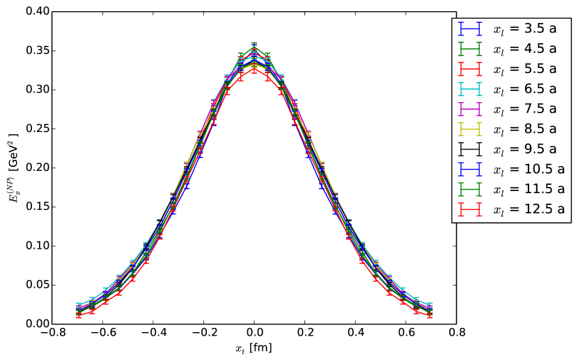
Figure 5: Transverse cross sections of the non-perturbative field $E_{x}^{\rm NP}(x_{t})$ at $\beta=6.370$, $d=0.85$ fm, for several values of $x_{l}$.

In Table 2 we also compare the values of the measured longitudinal chromoelectric field $E_{x}$ with those of the non-perturbative field $E_{x}^{\rm NP}$ on the axis at the midpoint between the quark and antiquark, for all ten values of their separation $d$. Given that $E^{\rm NP}_{x}$ is almost uniform along the axis, $E^{\rm NP}_{x}=E_{x}^{\rm NP}(x_{l},x_{t}=0)$ at all points $x_{l}$ on the axis for all distances larger than approximately $0.1-0.2~{}$ fm from the quark sources.

4 Non-perturbative content of the flux tube: the curl method

While the Coulomb field (5) gives a good description of the transverse components of the chromoelectric field when the distance from the sources is not too small, it does not give a good description at smaller distances, approximately two lattice spacings from the sources. This can be either the result of the non-spherical form of the effective charges, or an effect introduced by the discrete lattice.

To extract the confining part of the chromoelectric field in the data it is then preferable to have a procedure which avoids the use of an explicit fitting function, and which can work close to the quark sources. With this aim in mind we use the following two steps to separate the field into ’perturbative’ and ’non perturbative’ components.

1. We identify the transverse component $E_{y}$ of the simulated field with the transverse component $E^{\rm C}_{y}$ of the perturbative field, $E^{\rm C}_{y}\equiv E_{y}$.

2. We impose the condition that the perturbative field is irrotational, curl $\vec{E}^{\rm C}=0$.

Condition (1) implies that the nonperturbative field is purely longitudinal, ${E}^{\rm NP}_{y}=0$. Condition (2) will then fix the longitudinal component ${E}^{\rm C}_{x}$ of the perturbative field as well as the longitudinal component $E^{\rm NP}_{x}=E_{x}-E^{\rm C}_{x}$ of the non-perturbative field.

To implement the irrotational condition (2), taking into account that the fields are measured at discrete lattice points, the sum of the measured fields along any closed lattice path is zero. For example, on a plaquette this amounts to

$$E_{x}^{\rm C}(x,y)+E_{y}^{\rm C}(x+1,y)-E_{x}^{\rm C}(x,y+1)-E_{y}^{\rm C}(x,y)=0\ .$$ (6)

One can easily solve this equation for $E_{x}^{\rm C}$ obtaining

$$E_{x}^{\rm C}(x,y)=\sum_{y^{\prime}=y}^{y_{\mathrm{max}}}\left(E_{y}(x,y^{\prime})-E_{y}(x+1,y^{\prime})\right)+E_{x}^{\rm C}(x,y_{\mathrm{max}}+1)\ .$$ (7)

This of course leaves one unknown on each transverse slice of the field – the value of $E_{x}^{\rm C}(x,y_{\mathrm{max}}+1)$, but if the value of $y_{\max}$ is large enough, the perturbative field at that distance should already be small, so in our analysis we just put $E_{x}^{\rm C}(x,y_{\mathrm{max}}+1)=0$. To check that this indeed makes a little change to our results, we have used a separate procedure in which we fixed $E_{x}^{\rm C}(x,y_{\mathrm{max}}+1)=E_{x}$, in practice making $E_{x}^{\rm NP}=0$ at the largest transverse distance. This procedure gave similar results.

After the estimation of the perturbative longitudinal field $E_{x}^{\rm C}$ one can subtract it from the total field, obtaining the non-perturbative component (see Fig. 6). One can see that the non-perturbative part of the flux tube exhibits very little change along the line connecting the quark-antiquark pair; even at the smallest distances from the sources the non-perturbative field remains smooth (This is seen more clearly in Fig. 7).

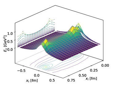
(a) $E_{x}(x_{t},x_{l})$

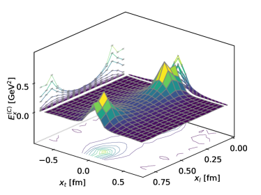
(b) $E_{x}^{\rm C}(x_{t},x_{l})$

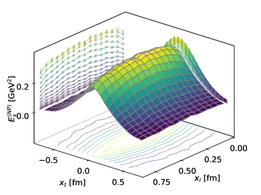
(c) $E_{x}^{\rm NP}(x_{t},x_{l})$

Figure 6: Surface and contour plots for the longitudinal components of the full, perturbative and non-perturbative chromoelectric field obtained by using the curl procedure at $\beta=6.370$ and $d=0.85~{}$fm. All plotted quantities are in physical units.

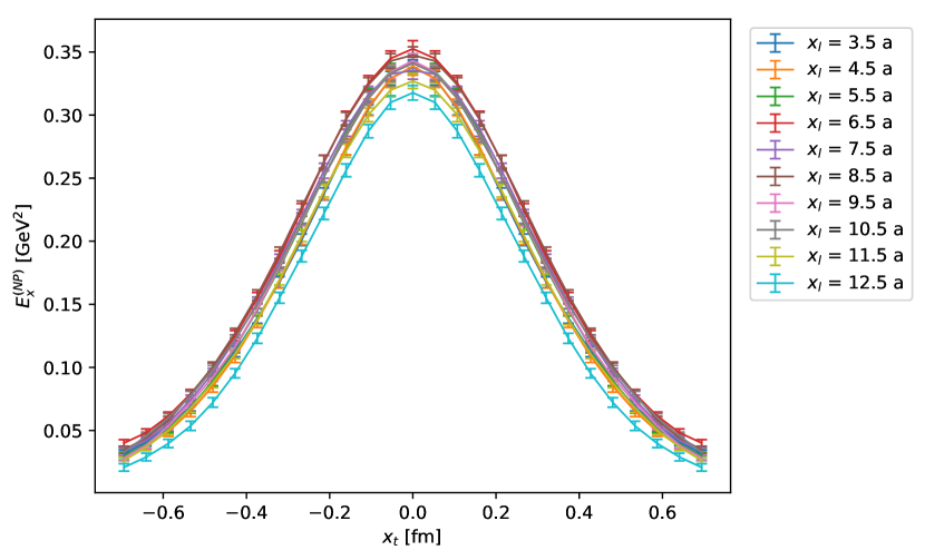
Figure 7: Transverse cross sections of the non-perturbative field obtained by using the curl procedure $E_{x}^{\rm NP}(x_{t})$ at $\beta=6.370$, $d=0.85$ fm, for several values of $x_{l}$.

Table 3: The Clem parameters describing the non-perturbative field transverse section going through the midpoint between the quark and antiquark positions. The data for the fit is obtained using the curl subtraction method, taking the perturbative field at $y_{\mathrm{max}+1}$ equal to zero.

$\beta$	$d$ [fm]	$\varphi$	$\mu$ [fm-1]	$\alpha$	$\kappa$	$\chi^{2}_{r}$
$6.47466$	$0.37$	$3.474(4)$	$4.999(9)$	$1.192(4)$	$0.808(4)$	$318$
$6.333$	$0.45$	$3.83(3)$	$5.30(6)$	$1.55(3)$	$0.576(15)$	$12.0$
$6.240$	$0.51$	$4.028(11)$	$6.039(26)$	$2.141(20)$	$0.375(5)$	$43.5$
$6.500$	$0.54$	$4.370(15)$	$5.71(4)$	$2.02(3)$	$0.406(9)$	$4.46$
$6.539$	$0.69$	$4.50(7)$	$6.25(20)$	$2.47(16)$	$0.309(27)$	$0.03$
$6.370$	$0.85$	$5.40(25)$	$6.7(9)$	$4.0$(1.1)	$0.17(7)$	$0.06$
$6.299$	$0.94$	$5.2(4)$	$7.8$(1.9)	$5.5$(2.8)	$0.10(7)$	$0.02$
$6.240$	$1.02$	$8.0(7)$	$4.4(8)$	$2.4(9)$	$0.33(17)$	$0.18$
$6.218$	$1.06$	$6.6(7)$	$6.0$(1.8)	$4.0$(2.4)	$0.16(13)$	$0.05$
$6.136$	$1.19$	$5.5$(1.6)	$81(27)$	7(5)${}\times 10^{2}$	8(9)${}\times 10^{-5}$	$0.17$

Table 4: The string tension estimated using the non-perturbative field from the curl procedure by employing different methods (from left to right: numerical integration of the field, analytical integration of the Clem function with parameters given in Table 3, estimation of fields at sources). In the last column we report also the value of the string tension obtained by numerically integrating Eq. (8) and using the non-perturbative field from the Coulomb subtraction $E_{x}^{\rm Coulomb}$.

$\beta$	$d$ [fm]	$\sqrt{\sigma_{\rm int}}$ [GeV]	$\sqrt{\sigma_{\rm Clem}}$ [GeV]	$\sqrt{\sigma_{\rm 0}}$ [GeV]	$\sqrt{\sigma_{\rm Coulomb}}$ [GeV]
$6.47466$	$0.37$	$0.4591(3)$	$0.4659(3)$	$0.53426(22)$	-
$6.333$	$0.45$	$0.5020(19)$	$0.5045(20)$	$0.5313(6)$	-
$6.240$	$0.51$	$0.5409(10)$	$0.5430(10)$	$0.5340(4)$	-
$6.500$	$0.54$	$0.5582(9)$	$0.5687(10)$	$0.5410(7)$	$0.491(25)$
$6.539$	$0.69$	$0.583(4)$	$0.596(5)$	$0.5526(28)$	$0.468(4)$
$6.370$	$0.85$	$0.633(16)$	$0.640(17)$	$0.528(7)$	$0.412(17)$
$6.299$	$0.94$	$0.617(23)$	$0.620(24)$	$0.527(11)$	$0.598(7)$
$6.240$	$1.02$	$0.75(4)$	$0.77(4)$	$0.520(17)$	$0.616(7)$
$6.218$	$1.06$	$0.69(4)$	$0.62(3)$	$0.482(19)$	$0.599(24)$
$6.136$	$1.19$	$0.67(11)$	$0.67(12)$	$0.56(5)$	$0.593(28)$

Table 5: The flux tube width estimated using the non-perturbative field from the curl procedure by employing different methods (from left to right: numerical integration of the field, analytical integration of the Clem function with parameters given in Table 3). In the last column we report also the value of the width obtained by numerically integrating Eq. (12) and using the non-perturbative field from the Coulomb subtraction $E_{x}^{\rm Coulomb}$.

$\beta$	$d$ [fm]	$\sqrt{w^{2}_{\rm int}}$ [fm]	$\sqrt{w^{2}_{\rm Clem}}$ [fm]	$\sqrt{w^{2}_{\rm Coulomb}}$ [fm]
$6.47466$	$0.37$	$0.31696(6)$	$0.4795(6)$	-
$6.333$	$0.45$	$0.3598(7)$	$0.477(3)$	-
$6.240$	$0.51$	$0.3838(3)$	$0.4543(9)$	-
$6.500$	$0.54$	$0.31716(15)$	$0.4727(18)$	$0.313(11)$
$6.539$	$0.69$	$0.3061(5)$	$0.457(6)$	$0.3020(23)$
$6.370$	$0.85$	$0.3712(24)$	$0.497(21)$	$0.343(16)$
$6.299$	$0.94$	$0.393(5)$	$0.483(29)$	$0.384(7)$
$6.240$	$1.02$	$0.448(6)$	$0.63(5)$	$0.417(11)$
$6.218$	$1.06$	$0.444(9)$	$0.56(5)$	$0.448(21)$
$6.136$	$1.19$	$0.43(7)$	$0.46(6)$	$0.51(4)$

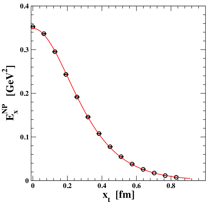
Figure 8: The Clem fit (Eq. (9) to the non-perturbative chromoelectric field $E_{x}^{\rm NP}$ obtained from the curl procedure for $\beta=6.240$, $d=0.51\,{\mathrm{fm}}$, $x_{l}=3a$.

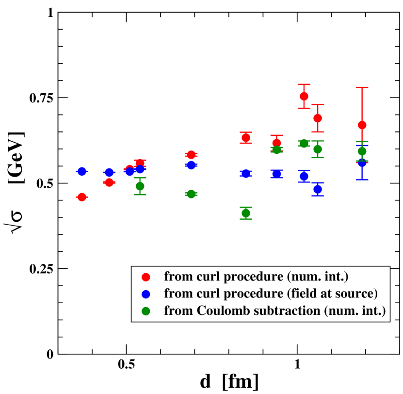
Figure 9: The square root of the string tension obtained using several different procedures: (i) by numerical integration of Eq. ((8) with the non-perturbative field obtained from the curl procedure (Section 4); (ii) from the non-perturbative field obtained from the curl procedure evaluated and evaluated at sources; (iii) by numerical integration of Eq. (8) with the non-perturbative field obtained from the Coulomb subtraction (Eq. (4)).

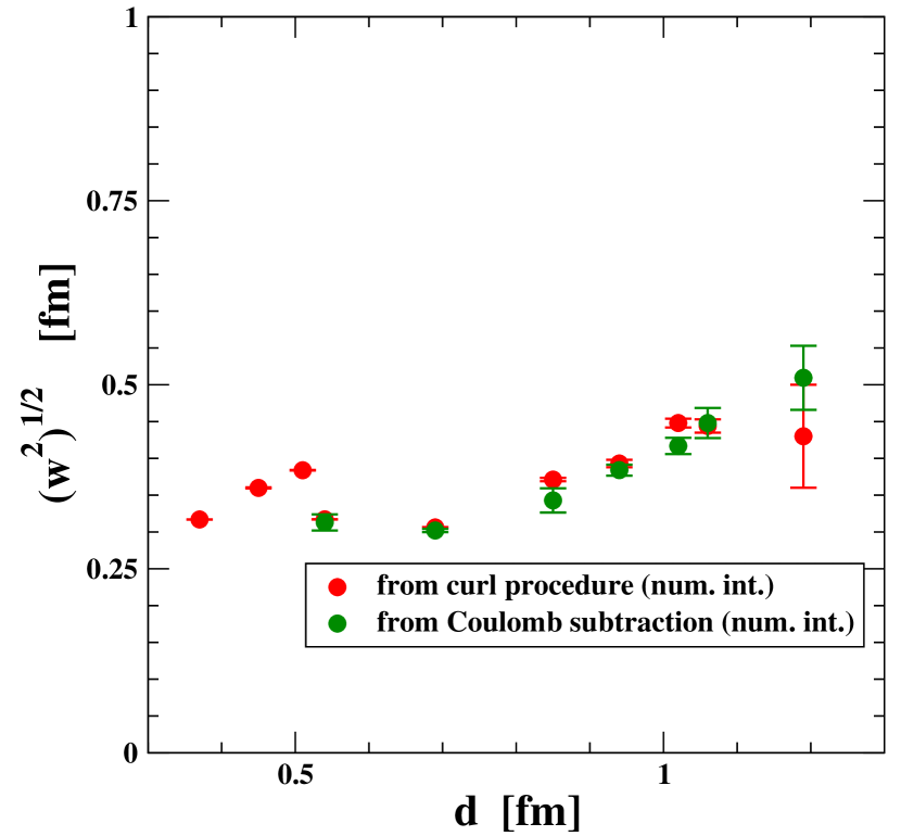
Figure 10: The mean square width of the flux tube obtained using several different procedures: (i) by numerical integration of Eq. (12) with the non-perturbative field obtained from the curl procedure (Section 4); (ii) by numerical integration of Eq. (8) with the non-perturbative field obtained from the Coulomb subtraction (Eq. (4))

5 The string tension and the width of the flux tube

The forces between charged particles in electrodynamics are determined by a stress tensor $T_{\mu\nu}$ constructed from fields $F_{\mu\nu}$ satisfying Maxwell’s equations (see Eq. (12.113) in Ref. jackson_classical_1999 ). Similarly, the force between quarks and antiquarks in Yang Mills theory is determined by the stress tensor $T_{\mu\nu}$, Eq. (13), constructed from the field tensor $F_{\mu\nu}$ obtained from our simulations.

The quark-antiquark force $\vec{F}$ is then the integral of the longitudinal component $T_{xx}=(E_{x}(x_{l}=d/2,x_{t}))^{2}/2$ of the stress tensor over the median plane $x=d/2$ bisecting the line connecting the quarks, Eq. (20). The non-perturbative quark-antiquark force $\vec{F}_{\rm NP}=-\hat{e}_{x}\sigma$ determining the string tension $\sigma$ has the corresponding expression in terms of the non-perturbative longitudinal component of the stress tensor $T^{\rm NP}_{xx}=(E^{\rm NP}_{x}(x_{l}=d/2,x_{t}))^{2}/2\equiv(E_{x}^{\rm NP})^{2}(x_{t}))/2.$

The square root of the string tension is then equal to

$$\sqrt{\sigma}=\sqrt{\int d^{2}x_{t}\frac{(E^{\rm NP}_{x})^{2}(x_{t})}{2}}.$$ (8)

We have evaluated the integral (Eq. (8) ) in two ways:

1. by direct numerical integration, using the values of $E_{x}^{\rm NP}$ determined by our simulations, and

2. analytically, by fitting the numerical data for the transverse distribution of $E_{x}^{\rm NP}(x_{t})$ as in Cardaci:2010tb ; Cea:2012qw ; Cea:2013oba ; Cea:2014uja ; Cea:2014hma to the Clem parameterization of the field surrounding a magnetic vortex in a superconductor Clem:1975aa .

   $$E_{x}^{\rm NP}(x_{t})=\frac{\phi}{2\pi}\frac{\mu^{2}}{\alpha}\frac{K_{0}[(\mu^{2}x_{t}^{2}+\alpha^{2})^{1/2}]}{K_{1}[\alpha]}\;,$$ (9)

   where $\phi,\mu$ and $\alpha$ are fitting parameters. In the dual superconducting model 'tHooft:1976ep ; Mandelstam:1974pi ; Ripka:2003vv ; Kondo:2014sta $\lambda=\frac{1}{\mu}$ is the penetration depth and

   $$\kappa=\frac{\sqrt{2}}{\alpha}\left[1-K_{0}^{2}(\alpha)/K_{1}^{2}(\alpha)\right]^{1/2}\,,$$ (10)

   is the Landau-Ginzburg parameter characterizing the type of superconductor.

Figure (8) shows an example of the fit of the data to the Clem functional form Eq. (9). for the transverse distribution of $E_{x}^{\rm NP}(x_{t})$, obtained using the curl procedure.

We can obtain a second expression for the string tension by utilizing the result  Brambilla:2000gk ; brambilla2019static that the force on a quark is equal to the value of the chromoelectric field at the position of the quark. The string tension is then equal to the corresponding value of the confining part of the chromoelectric field

$$\sigma=E^{\rm NP}_{x}(x_{l}=0,x_{t}=0).$$ (11)

Eqs. (8) and (11) provide two independent ways to extract the string tension from simulations. As mentioned earlier, we must use the curl method to isolate the confining field to extract the string tension by Eq. (11).

To obtain additional information about the structure of the chromoelectric flux tube we have calculated the mean square root width:

$$\sqrt{w^{2}}=\sqrt{\frac{\int d^{2}x_{t}\,x_{t}^{2}E_{x}(x_{t})}{\int d^{2}x_{t}\,E_{x}(x_{t})}}.$$ (12)

Just as we have evaluated the integral (8) for the string tension, we have evaluated the integral (12) for the mean square root width both numerically, using the data for $E_{x}^{\rm NP}(x_{t})$, and analytically, in terms of Clem parameters, fitting the longitudinal component of $E_{x}^{\rm NP}(X_{t})$ in the median plane to the Clem parametrization ((9)). The results of that fit are given in Table 3. In most cases the parametrization in Eq. (9) gives a good description of the field, shown by the values of $\chi^{2}_{r}$, though the parameters themselves are somewhat unstable, which reflects the strong correlation between the parameter estimates.

We compared two different methods for calculating the integrals in Eqs.  (8) and (12). First, we carried out the numeric integration in Eqs. (8) and (12), respectively, postulating the rotational symmetry of the field. This approach was repeated for both the non-perturbative field obtained using the “curl procedure” (resulting in $\sqrt{\sigma_{\rm int}}$ and $\sqrt{w^{2}_{\rm int}}$) and the field obtained using Coulomb subtraction (resulting in $\sqrt{\sigma_{\rm Coulomb}}$ and $\sqrt{w^{2}_{\rm Coulomb}}$). Next we calculated the values of the string tension and the mean square root width using the Clem parameters given in Table 3 to get the values denoted as $\sqrt{\sigma_{\rm Clem}}$ and $\sqrt{w^{2}_{\rm Clem}}$.

(One remark should be made for the width – while we know that the value of $E_{x}^{\rm C}(x,y_{\mathrm{max}}+1)$ in Eq. (7) is small ($O(y_{\mathrm{max}}^{-2})$), in the numerator of Eq. 12 this small constant will be multiplied by $y^{2}$ ($y^{3}$ after the integration over polar angle), which will cause the error introduced to increase with $y_{\max}$. Indeed, the comparison with the analysis done taking $E_{x}^{\rm NP}(x,y_{\rm max})=0$ shows large discrepancies in this case.)

Finally, we evaluated expression (11) for the string tension, $\sigma=E^{\rm NP}_{x}(x_{l}=0,x_{t}=0)$, using the curl method to determine the magnitude of the non-perturbative field at the sources.

Our results are gathered in Tables 4 and 5, where we use the notation $\sigma_{0}\equiv E^{\rm NP}_{y}(x_{l}=0,~{}x_{t}=0)$ and in Fig. (9). The data shown in Fig. (9) give a consistent value of $\sqrt{\sigma}$ for all values of the separation $d$, with scatter that increases with $d$ as the resolution diminishes. The values of $\sqrt{\sigma}$ lie close to $0.465$ GeV, the value used in the parameterization Ref. Necco:2001xg

Let us review the basis of our calculations. Our hypothesis is that the string tension is determined by the field $\vec{E}$ we measured (the ’Maxwell’ mechanism). We have determined $\sigma$ from both the transverse structure of the flux tube (Eq.  (8)) and its longitudinal structure (Eq. 11) ) as shown in Fig. (6(c)), in which the non-perturbative field has been isolated.

We emphasize that, as discussed in Section (3), the ’Maxwell’ mechanism cannot be used to obtain the Coulomb correction to the string tension. This implies that the fluctuating fields not measured in our simulations must contribute to the Coulomb force.

On the other hand, the Coulomb correction has been obtained by recent direct simulations of the stress energy-momentum tensor in Yang Mills theory Yanagihara:2018qqg . The Yang Mills stress tensor accounts for the contributions of fluctuating fields but cannot be directly related to measured fields, in contrast to the Maxwell stress tensor $T_{xx}=(1/2)E_{x}^{2}$, determining the string tension. (See Eq. (A).)

6 Conclusions and outlook

In this paper we have determined the spatial distribution in three dimensions of all components of the color fields generated by a static quark-antiquark pair. We have found that the dominant component of the color field is the chromoelectric one in the longitudinal direction, i.e. in the direction along the axis connecting the two quark sources. This feature of the field distribution has been known for a long time. However, the accuracy of our numerical results allowed us to go far beyond this observation. First, we could confirm that, as observed in Baker:2018mhw , all the chromomagnetic components of the color field are compatible with zero within the statistical uncertainties. Second, the chromoelectric components of the color fields in the directions transverse to the axis connecting the two sources, though strongly suppressed with respect to the longitudinal component, are sufficiently greater than the statistical uncertainties that they can be nicely reproduced by a Coulomb-like field generated by two sources with opposite charge (everywhere except in a small region around the sources).

In Ref. Baker:2018mhw we subtracted this Coulomb-like field from the simulated chromoelectric field to obtain a non-perturbative field $\vec{E}^{\rm NP}$ according to Eq. (4) and found that the dependence of the resulting longitudinal component of $\vec{E}^{\rm NP}$ on the distance $x_{t}$ from the axis is independent of the position $x_{l}$ along the axis, except near the sources, thus suggesting that the non-perturbative field found in this way from lattice simulations can be identified as the confining field of the QCD flux tube.

In this work we have improved the approach of Ref. Baker:2018mhw by presenting a new procedure to subtract the Coulomb-like field, which does not rely on any preconception about its analytic form, but is based only on the requirement that its curl is equal to zero.

Moreover, we have carefully analyzed the spatial distribution of the subtracted, non-perturbative part of the longitudinal chromoelectric field to extract from it some relevant parameters of the flux tube, such as the mean width and the string tension, both by means of a fully numerical, model-independent procedure and by a prior interpolation with the dual version of the Clem function for the magnetic field in a superconductor.

We have also used our determinations of the color field components to construct the ‘Maxwell’ stress tensor. Details about its determination and a comparison with the recent literature about this topic Yanagihara:2018qqg are presented in A.

In conclusion, we have shown that the separation of the chromoelectric field into perturbative and non-perturbative components can be obtained by directly analyzing lattice data on color field distributions between static quark sources, with no need of model assumptions. To the best of our knowledge, this separation between perturbative and non-perturbative components has not been carried out previously. It provides new understanding of the chromoelectric field surrounding the quarks. We have used the non-perturbative field to calculate the string tension and the spatial distribution of the energy-momentum tensor surrounding the static quarks, under the assumption that the fluctuating color fields not measured in our simulations do not contribute to the string tension. The extension of our approach to the case of QCD with dynamical fermions with physical masses and at non-zero temperature and baryon density is straightforward Cea:2015wjd .

Appendix A The ‘Maxwell” stress tensor

In this Appendix we consider the “Maxwell” energy-momentum tensor $T_{\mu\nu}$ as a function of the field tensor $F_{\mu\nu}$ characterizing the SU(3) flux tube, which is in its turn defined in terms of the gauge invariant correlation function $\rho^{\rm conn}_{W,\mu\nu}$ of Eqs. (1) and (2) and points in a single color direction parallel to the color direction of the source (which is determined dynamically). Its six tensor components (the electric and magnetic fields $\vec{E}$ and $\vec{B}$) correspond to the six orientations of the plaquette $U_{P}$ relative to that of the Wilson loop (see Fig. 1(a)).

The simulated fields $\vec{E}$ and $\vec{B}$ have the space-time symmetries of the Maxwell fields of electrodynamics, while carrying color charge in a single direction in color space. The energy-momentum tensor $T_{\mu\nu}$ lies in the same direction in color space of the simulated fields $\vec{E}$ and $\vec{B}$ and has the (Euclidean) Maxwell form:

$$T_{\mu\nu}=F_{\mu\alpha}F_{\alpha\nu}-g_{\mu\nu}F_{\alpha\beta}F_{\alpha\beta}/4\;.$$ (13)

Its spatial components $\mu=i,\nu=j$, with $i,j=1,2,3$ determine the Maxwell stress tensor:

$$T^{\rm Maxwell}_{ij}=-T_{ij}\;.$$ (14)

Taking $\mu=i$ and $\nu=j\neq i$ in Eq. (13) gives

$$T_{ij}^{\rm Maxwell}=-T_{ij}=E_{i}E_{j}+B_{i}B_{j}-\delta_{ij}(E^{2}+B^{2})/2\;,$$ (15)

while the diagonal time component $-T_{44}$ of $T_{\mu\nu}$ determines the energy density,

$$-T_{44}=\frac{1}{2}(E^{2}+B^{2})\;.$$ (16)

We use cylindrical coordinates $(x,~{}r,~{}\theta)$, $r\equiv\sqrt{y^{2}+z^{2}}$, $\tan\theta\equiv z/y$, and the corresponding unit vectors $\hat{e}_{r}$, $\hat{e}_{\theta}$:

$$\hat{e}_{r} = \hat{e}_{y}\cos\theta+\hat{e}_{z}\sin\theta\;,$$ (17)

$$\hat{e}_{\theta} = -\hat{e}_{y}\sin\theta+\hat{e_{z}}\cos\theta$$ (18)

($x$ is the longitudinal direction of the flux tube, i.e. the axis along which the static sources are located).

The force exerted by the antiquark on the quark can be expressed, by means of the stress tensor, as a surface force $\vec{F}$ acting on the infinite plane $x=\frac{d}{2}$ bisecting the line connecting the pair:

$$\vec{F}_{j}=\int\int dy~{}dz~{}\hat{n}_{i}T^{\rm Maxwell}_{ij}(x=d/2,~{}y,~{}z)\;,$$ (19)

where $\hat{n}=-\hat{e}_{x}$ is the outward normal to the region $x>\frac{d}{2}$ containing the quark. The only non-vanishing component of the quark-antiquark force $\vec{F}$ is longitudinal, so

$$\vec{F}=-\int\int dy~{}dz~{}\hat{e}_{x}T_{xx}(x=d/2,~{}y,~{}z).$$ (20)

Using the components in Eq. (15) of $T_{ij}^{\rm Maxwell}$, and taking into account that the measured magnetic field $B$ is compatible with zero

$$-T_{xx} = \frac{1}{2}(E_{x}^{2}-E_{r}^{2}),\;\;\;\;\;E_{r}^{2}=E_{y}^{2}+E_{z}^{2}\;,$$

$$-T_{xy} = E_{x}E_{y}\;,$$ (21)

$$-T_{xz} = E_{x}E_{z}\;,$$

in Eq. (19) gives

$$\vec{F}=-\int_{o}^{2\pi}d\theta\int_{0}^{\infty}r~{}dr[\hat{e}_{x}\frac{(E_{x}^{2}-E_{r}^{2})}{2}+\hat{e}_{r}E_{x}E_{r}]\;.$$ (22)

The angular average over the radial vector $\hat{e}_{r}$ in Eq. (22) vanishes. Furthermore by symmetry the transverse field $E_{r}$ on the mid-plane $x=\frac{d}{2}$ vanishes, so that the quark-antiquark force in Eq. (22) becomes

$$\vec{F}=-2\pi\int_{0}^{\infty}rdr\frac{E_{x}^{2}(r)}{2}\hat{e}_{x}\;.$$ (23)

Replacing $E_{x}(r)$ by the non-perturbative field $E_{x}^{\rm NP}(r)$ in Eq. (23) gives the non-perturbative quark-antiquark force $\vec{F}_{\rm NP}$,

$$\vec{F}_{\rm NP}=-\sigma\hat{e}_{x}\;,\;\;\;\sigma=2\pi\int_{0}^{\infty}rdr\frac{(E_{x}^{\rm NP}(r))^{2}}{2}\;.$$ (24)

Eq. (24) determines the string tension $\sigma$ in terms of the longitudinal component of the non-perturbative field $E_{x}^{\rm NP}(r)$, the confining component of the SU(3) flux tube. We have already presented it, in a slightly different notation, in Eq. (8).

Using Eqs. (17) and (18) in Eq. (15) we can obtain the components of the Maxwell stress tensor in cylindrical coordinates:

$$-T_{rr}(x,r) = -(\hat{e}_{r})_{i}T_{ij}(\hat{e_{r}})_{j}~{}=~{}-\frac{1}{2}(E_{x}^{2}-E_{r}^{2})\;,$$ (25)

$$-T_{\theta\theta}(x,r) = -(\hat{e}_{\theta})_{i}T_{ij}(\hat{e_{\theta}})_{j}~{}=~{}-\frac{1}{2}(E_{x}^{2}+E_{r}^{2})\;,$$ (26)

$$-T_{xx}(x,r) = -(\hat{e}_{x})_{i}T_{ij}(\hat{e_{r}})_{j}~{}=~{}~{}~{}~{}~{}\frac{1}{2}(E_{x}^{2}-E_{r}^{2})\;,$$ (27)

$$-T_{xr}(x,r) = -(\hat{e}_{x})_{i}T_{ij}(\hat{e_{r}})_{j}~{}=~{}~{}~{}~{}E_{x}E_{r}\;.$$ (28)

The remaining non-vanishing component of $T_{\mu\nu}$ is the energy density $T_{44}$,

$$-T_{44}(x,r) = \frac{1}{2}(E_{x}^{2}+E_{r}^{2})\;.$$ (29)

Eqs. (25)-(29) express all components of the stress tensor in terms of the simulated color fields $E_{x}(x,r)$ and $E_{r}(x,r)=\sqrt{E_{y}^{2}+E_{z}^{2}}$. On the symmetry plane $x=\frac{d}{2}$, $E_{r}=0$ and Eqs. (25)-(29) reduce to

$$T_{44}(r) = T_{xx}(r)=-\frac{E_{x}^{2}(r)}{2}\;,$$ (30)

$$T_{rr}(r) = T_{\theta\theta}(r)~{}=\frac{E_{x}^{2}(r)}{2}\;.$$ (31)

Further, we note that the trace of the stress tensor $T_{\mu\nu}$ evaluated from Eqs. (25)-(29) vanishes independently of the simulated flux-tube fields $E_{x}(x,r)$ and $E_{r}(x,r)$:

$$T_{44}(x,r)+T_{xx}(x,r)+T_{rr}(x,r)+T_{\theta\theta}(x,r)=0\;.$$ (32)

We have calculated the non-perturbative content of $T_{rr}$ on the symmetry plane (where $T_{rr}=T_{\theta\theta}=-T_{44}=-T_{xx}$) versus $r$ for three different values of the quark-antiquark distance: $d=0.51$ fm (at $\beta=6.240$), $d=0.69$ fm (at $\beta=6.539$) and $d=0.95$ fm (at $\beta=6.299$). Results are presented in Fig. 11, where also the full (non-perturbative plus Coulomb) content of $T_{rr}$ is shown.

The width of the energy density distribution $T^{\rm NP}_{44}$ can be obtained through Eq. (12), with $E^{\rm NP}_{x}$ replaced by $T^{\rm NP}_{44}$ as given in Eq. (30); results are presented in Table 6. Since $T_{44}^{\rm NP}$ is proportional to $\left(E_{x}^{\rm NP}\right)^{2}$ the width of the $T_{44}^{\rm NP}$ component of the Maxwell stress tensor obtained from the nonperturbative field given in Table 6 is systematically smaller than the width of the nonperturbative part of the longitudinal chromoelectric field component $E_{x}^{\rm NP}$ given in Table 5. (The square of the field decreases more rapidly with distance than the field itself.)

We now compare the above results obtained using our measured flux tube fields to evaluate the ’Maxwell’ energy-momentum tensor $T_{\mu\nu}$ with the corresponding results of recent direct simulations Yanagihara:2018qqg of the expectation value of the energy momentum tensor $T_{\mu\nu}^{\rm YM}$ in the presence of a quark-antiquark pair. The latter simulations, which measure the energy and stresses in all color directions directly, were carried out in the plane midway between the quark and the antiquark, for three values of their separation.

The tensor $T_{\mu\nu}^{\rm YM}$ has the form Suzuki:2013gza

$$T_{\mu\nu}=F_{\mu\alpha}^{a}F_{\alpha\nu}^{a}-g_{\mu\nu}F_{\alpha\beta}^{a}F_{\alpha\beta}^{a}/4\,,$$ (33)

where $F_{\mu\nu}^{a}$ is the Yang-Mills field tensor in the adjoint representation of SU(3),

$$F_{\mu\nu}^{a}=\partial_{\mu}A_{\nu}^{a}-\partial_{\nu}A_{\mu}^{a}+gf_{abc}A_{\mu}^{b}A_{\nu}^{c}\,,$$ (34)

where $f_{abc}$ are the structure constants of the SU(3) algebra. In our definition the field is squared after color projection, whereas in Eq. (33) the sum over color components is taken after squaring. Moreover, the stress tensor in Ref. Yanagihara:2018qqg is renormalized (this motivates the superscript $R$ in the formulas below).

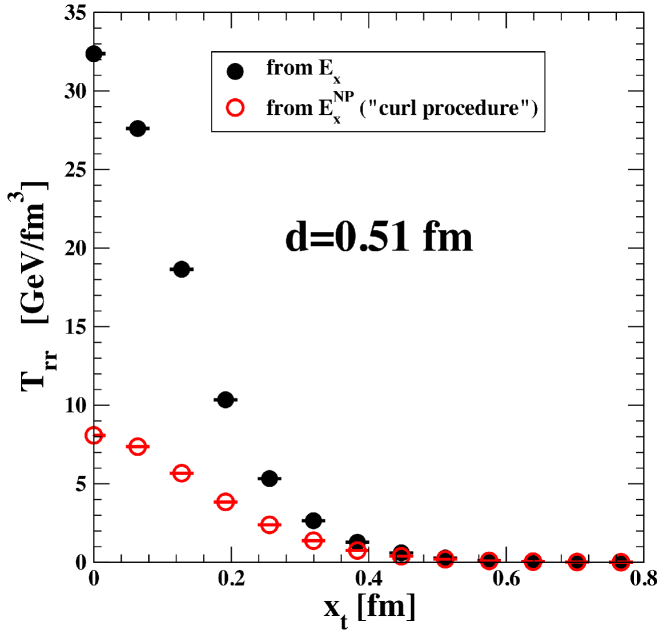
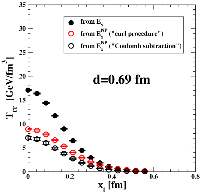
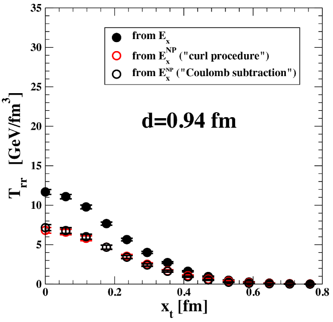
Figure 11: The diagonal components of the Maxwell stress tensor recovered from the full field $E_{x}$ (filled circles) and non-perturbative field $E_{x}^{(\rm NP)}$ (empty circles) for $d=0.51$ fm (top), $d=0.69$ fm (middle), and $d=0.95$ fm (bottom).

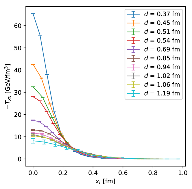
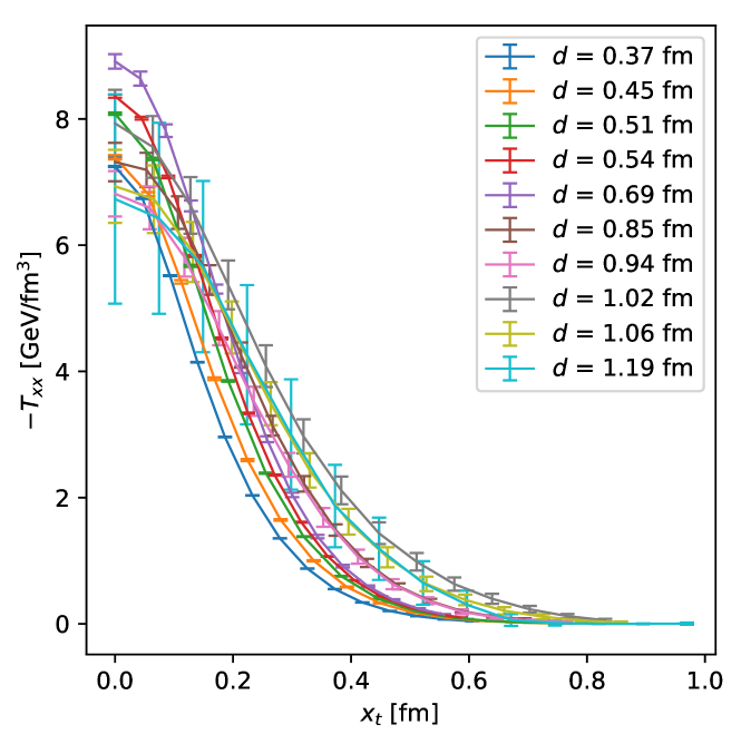
Figure 12: Comparison of the diagonal components of the “Maxwell” stress tensor for the different quark-antiquark separations, recovered from the full field $E_{x}$ (top) and from the non-perturbative field $E_{x}^{(\rm NP)}$ (bottom).

Table 6: The width of the diagonal component of the Maxwell stress tensor recovered from the full field $E_{x}$ ($\sqrt{w^{2}_{\rm Full}}$) and non-perturbative field $E_{x}^{(\rm NP)}$ ($\sqrt{w^{2}_{\rm NP}}$).

$\beta$	$d$ [fm]	$\sqrt{w^{2}_{\rm Full}}$ [fm]	$\sqrt{w^{2}_{\rm NP}}$ [fm]
$6.47466$	$0.37$	$0.18751(4)$	$0.24438(9)$
$6.333$	$0.45$	$0.2148(3)$	$0.2637(7)$
$6.240$	$0.51$	$0.23014(10)$	$0.26925(27)$
$6.500$	$0.54$	$0.22597(15)$	$0.25572(21)$
$6.539$	$0.69$	$0.2360(6)$	$0.2511(8)$
$6.370$	$0.85$	$0.2833(25)$	$0.298(3)$
$6.299$	$0.94$	$0.300(3)$	$0.306(6)$
$6.240$	$1.02$	$0.326(6)$	$0.360(9)$
$6.218$	$1.06$	$0.326(7)$	$0.345(10)$
$6.136$	$1.19$	$0.320(20)$	$0.319(27)$

In Yanagihara:2018qqg the expectation value of the energy-momentum tensor in the background of a quark-antiquark pair is denoted by $\left\langle~{}T_{ij}^{R}(r)~{}\right\rangle_{Q\bar{Q}}$. We will use this notation in comparing our results (30) and (31) with that work.

In Yanagihara:2018qqg the $r$ dependence of the components of $\left\langle~{}T_{\mu\nu}^{R}(r)~{}\right\rangle_{Q\bar{Q}}$ was plotted for the 3 values of the quark-antiquark separation for which simulations were made, and these ’noticeable’ features of the results were pointed out:

1. Approximate degeneracies between temporal and longitudinal components and between radial and angular components are found for a wide range of $r$;

   $$\left\langle T_{44}^{R}(r)\right\rangle_{Q\bar{Q}}~{}\approx~{}\left\langle T_{xx}^{R}(r)\right\rangle_{Q\bar{Q}}~{}>~{}0\,,$$

   $$\left\langle T_{rr}^{R}(r)\right\rangle_{Q\bar{Q}}~{}\approx~{}\left\langle T_{\theta\theta}^{R}(r)\right\rangle_{Q\bar{Q}}~{}>~{}0.$$ (35)

   We emphasize that the two inequalities in Eq. (35) are general consequences of (30) and (31), independent of the values of the simulated field $E_{x}(x,r)$. In contrast, a recent study Yanagihara:2019foh of the stress tensor distribution in the Abelian Higgs model found that these relations could only be satisfied within a very narrow range of the model parameters .

2. The scale symmetry broken in the YM vacuum (the trace anomaly),

   $$\left\langle T_{44}^{R}(r)\right\rangle_{Q\bar{Q}}+\left\langle T_{xx}^{R}(r)\right\rangle_{Q\bar{Q}}$$

   $$+\left\langle T_{rr}^{R}(r)\right\rangle_{Q\bar{Q}}+\left\langle T_{\theta\theta}^{R}(r)\right\rangle_{Q\bar{Q}} ~{}<~{}0,$$

   is partially restored inside the flux tube.

3. Each component of the energy-momentum tensor at r=0 decreases as the separation becomes larger, while the transverse radius of the flux tube, typically about 0.2 fm, seems to increase for large separations Luscher:1980iy ; Gliozzi:2010zv ; Cardoso:2013lla , although the statistics are not sufficient to discuss the radius quantitatively.

   We see some indication of the increase in the width of the distributions of the diagonal components of the ’Maxwell’ stress tensor in Fig. (12) and Table (6) for all ten values of the quark-antiquark separation. However, this width is greater than 0.2 fm, the transverse radius of the flux tube estimated by Yanagihara:2018qqg .

Combining Eq. (35) with Eq. (2), we obtain

$$\left\langle T^{R}_{rr}(r)\right\rangle_{Q\bar{Q}}<-\left\langle T^{R}_{xx}(r)\right\rangle_{Q\bar{Q}}\;,$$ (37)

which can be clearly seen from Fig. 3 of Ref. Yanagihara:2018qqg , where the components of $\left\langle T_{ij}^{R}(r)\right\rangle_{Q\bar{Q}}$ were plotted.

The ’Maxwell’ stress tensor does not include the contributions to Eq. (33) of the fluctuating color fields not measured in our simulations. Comparison of the spatial distributions of the diagonal components of the Yang-Mills stress tensor with the corresponding distributions of the ’Maxwell’ stress tensor then provides a measure of the contributions of the fluctuating color fields.

References

- (1) J. Greensite, An Introduction to the Confinement Problem, Lecture Notes in Physics (Springer Berlin Heidelberg, 2011), ISBN 9783642143816, https://books.google.de/books?id=CP7_QooHo8wC
- (2) D. Diakonov, Nucl. Phys. Proc. Suppl. 195, 5 (2009), 0906.2456
- (3) O. Philipsen, H. Wittig, Phys. Rev. Lett. 81, 4056 (1998), [Erratum: Phys. Rev. Lett.83,2684(1999)], hep-lat/9807020
- (4) S. Kratochvila, P. de Forcrand, Nucl. Phys. Proc. Suppl. 119, 670 (2003), [,670(2002)], hep-lat/0209094
- (5) G.S. Bali, H. Neff, T. Duessel, T. Lippert, K. Schilling (SESAM), Phys. Rev. D71, 114513 (2005), hep-lat/0505012
- (6) M. Bander, Phys. Rept. 75, 205 (1981)
- (7) J. Greensite, Prog. Part. Nucl. Phys. 51, 1 (2003), hep-lat/0301023
- (8) G. Ripka, AIP Conf. Proc. 775, 262 (2005)
- (9) Y.A. Simonov (2018), 1804.08946
- (10) M. Fukugita, T. Niuya, Phys. Lett. B132, 374 (1983)
- (11) J.E. Kiskis, K. Sparks, Phys. Rev. D30, 1326 (1984)
- (12) J.W. Flower, S.W. Otto, Phys. Lett. B160, 128 (1985)
- (13) J. Wosiek, R.W. Haymaker, Phys. Rev. D36, 3297 (1987)
- (14) A. Di Giacomo, M. Maggiore, S. Olejnik, Phys. Lett. B236, 199 (1990)
- (15) A. Di Giacomo, M. Maggiore, S. Olejnik, Nucl. Phys. B347, 441 (1990)
- (16) P. Cea, L. Cosmai, Nucl. Phys. Proc. Suppl. 30, 572 (1993)
- (17) Y. Matsubara, S. Ejiri, T. Suzuki, Nucl. Phys. Proc. Suppl. 34, 176 (1994), hep-lat/9311061
- (18) P. Cea, L. Cosmai, Phys. Lett. B349, 343 (1995), hep-lat/9404017
- (19) P. Cea, L. Cosmai, Phys. Rev. D52, 5152 (1995), hep-lat/9504008
- (20) G.S. Bali, K. Schilling, C. Schlichter, Phys. Rev. D51, 5165 (1995), hep-lat/9409005
- (21) A.M. Green, C. Michael, P.S. Spencer, Phys. Rev. D55, 1216 (1997), hep-lat/9610011
- (22) P. Skala, M. Faber, M. Zach, Nucl.Phys. B494, 293 (1997), hep-lat/9603009
- (23) R.W. Haymaker, T. Matsuki, Phys. Rev. D75, 014501 (2007), hep-lat/0505019
- (24) A. D’Alessandro, M. D’Elia, L. Tagliacozzo, Nucl.Phys. B774, 168 (2007), hep-lat/0607014
- (25) M.S. Cardaci, P. Cea, L. Cosmai, R. Falcone, A. Papa, Phys.Rev. D83, 014502 (2011), 1011.5803
- (26) P. Cea, L. Cosmai, A. Papa, Phys.Rev. D86, 054501 (2012), 1208.1362
- (27) P. Cea, L. Cosmai, F. Cuteri, A. Papa, Flux tubes and coherence length in the SU(3) vacuum, in Proceedings, 31st International Symposium on Lattice Field Theory (Lattice 2013) (2013), Vol. LATTICE2013, p. 468, 1310.8423
- (28) P. Cea, L. Cosmai, F. Cuteri, A. Papa, Phys. Rev. D89, 094505 (2014), 1404.1172
- (29) P. Cea, L. Cosmai, F. Cuteri, A. Papa, PoS LATTICE2014, 350 (2014), 1410.4394
- (30) N. Cardoso, M. Cardoso, P. Bicudo, Phys. Rev. D88, 054504 (2013), 1302.3633
- (31) M. Caselle, M. Panero, R. Pellegrini, D. Vadacchino, JHEP 01, 105 (2015), 1406.5127
- (32) P. Cea, L. Cosmai, F. Cuteri, A. Papa, JHEP 06, 033 (2016), 1511.01783
- (33) P. Cea, L. Cosmai, F. Cuteri, A. Papa, Phys. Rev. D95, 114511 (2017), 1702.06437
- (34) E. Shuryak (2018), 1806.10487
- (35) C. Bonati, S. Calì, M. D’Elia, M. Mesiti, F. Negro, A. Rucci, F. Sanfilippo, Phys. Rev. D98, 054501 (2018), 1807.01673
- (36) A. Shibata, K.I. Kondo, S. Kato (2019), 1911.00898
- (37) M. Baker, P. Cea, V. Chelnokov, L. Cosmai, F. Cuteri, A. Papa, Eur. Phys. J. C79, 478 (2019), 1810.07133
- (38) R. Yanagihara, T. Iritani, M. Kitazawa, M. Asakawa, T. Hatsuda, Phys. Lett. B789, 210 (2019), 1803.05656
- (39) R. Yanagihara, M. Kitazawa, PTEP 2019, 093B02 (2019), 1905.10056
- (40) P. Bicudo, N. Cardoso, M. Cardoso, Phys. Rev. D 98, 114507 (2018)
- (41) L. Mueller, O. Philipsen, C. Reisinger, M. Wagner (2019), 1907.01482
- (42) N. Brambilla, A. Pineda, J. Soto, A. Vairo, Phys. Rev. D63, 014023 (2001), hep-ph/0002250
- (43) S. Necco, R. Sommer, Nucl. Phys. B622, 328 (2002), hep-lat/0108008
- (44) O. Kaczmarek, F. Zantow, Phys. Rev. D71, 114510 (2005), hep-lat/0503017
- (45) F. Karbstein, M. Wagner, M. Weber, Phys. Rev. D98, 114506 (2018), 1804.10909
- (46) D.S. Kuzmenko, Y.A. Simonov, Phys. Lett. B494, 81 (2000), hep-ph/0006192
- (47) A. Di Giacomo, H.G. Dosch, V.I. Shevchenko, Y.A. Simonov, Phys. Rept. 372, 319 (2002), hep-ph/0007223
- (48) N. Battelli, C. Bonati, Phys. Rev. D99, 114501 (2019), 1903.10463
- (49) A. Hasenfratz, F. Knechtli, Phys. Rev. D64, 034504 (2001), hep-lat/0103029
- (50) M. Falcioni, M. Paciello, G. Parisi, B. Taglienti, Nuclear Physics B 251, 624 (1985)
- (51) M. Luscher, Nucl. Phys. B180, 317 (1981)
- (52) J.D. Jackson, Classical electrodynamics, 3rd edn. (Wiley, New York, NY, 1999), ISBN 9780471309321, http://cdsweb.cern.ch/record/490457
- (53) J.R. Clem, Journal of Low Temperature Physics 18, 427 (1975), 10.1007/BF00116134
- (54) G. ’t Hooft, The confinement phenomenon in quantum field theory, in High Energy Physics, EPS International Conference, Palermo, 1975, edited by A. Zichichi (1975)
- (55) S. Mandelstam, Phys. Rept. 23, 245 (1976)
- (56) G. Ripka, Lect. Notes Phys. 639, 1 (2004)
- (57) K.I. Kondo, S. Kato, A. Shibata, T. Shinohara, Phys. Rept. 579, 1 (2015), 1409.1599
- (58) N. Brambilla, V. Leino, O. Philipsen, C. Reisinger, A. Vairo, M. Wagner (2019), 1911.03290
- (59) H. Suzuki, PTEP 2013, 083B03 (2013), [Erratum: PTEP2015,079201(2015)], 1304.0533
- (60) M. Luscher, G. Munster, P. Weisz, Nucl. Phys. B180, 1 (1981)
- (61) F. Gliozzi, M. Pepe, U.J. Wiese, Phys. Rev. Lett. 104, 232001 (2010), 1002.4888