Cosmology and dark matter

Abstract

Cosmology and astroparticle physics give strongest possible evidence for the incompleteness of the Standard Model of particle physics. Leaving aside misterious dark energy, which may or may not be just the cosmological constant, two properties of the Universe cannot be explained by the Standard Model: dark matter and matter-antimatter asymmtery. Dark matter particles may well be discovered in foreseeable future; this issue is under intense experimental investigation. Theoretical hypotheses on the nature of the dark matter particles are numerous, so we concentrate on several well motivated candidates, such as WIMPs, axions and sterile neutrinos, and also give examples of less motivated and more elusive candidates such as fuzzy dark matter. This gives an idea of the spectrum of conceivable dark matter candidates, while certainly not exhausting it. We then consider the matter-antimatter asymmetry and discuss whether it may result from physics at 100 GeV – TeV scale. Finally, we turn to the earliest epoch of the cosmological evolution. Although the latter topic does not appear immediately related to contemporary particle physics, it is of great interest due to its fundamental nature. We emphasize that the cosmological data, notably, on CMB anisotropies, unequivocally show that the well understood hot stage was not the earliest one. The best guess for the earlier stage is inflation, which is consistent with everything known to date; however, there are alternative scenarios. We discuss the ways to study the earliest epoch, with emphasis on future cosmological observations.

1 Introduction

It is a commonplace by now that cosmology and astroparticle physics, on the one side, and particle physics, on the other, are deeply interrelated. Indeed, the gross properties of the Universe – the existence of dark matter and the very presence of conventional, baryonic matter – call for the extension of the Standard Model of particle physics. A fascinating possibility is that the physics behind these phenomena is within reach of current or future terrestrial experiments. The experimental programs in these directions are currently intensely pursued.

Another aspect of cosmology, which currently does not apppear directly related to terrestrial particle physics experiments, is the earliest epoch of the evolution of the Universe. On the one hand, there is no doubt that the usual hot epoch was preceded by another, much less conventional stage. This knowledge comes from the study of inhomogeneities in the Universe through the measurements of CMB anisotropies, as well as matter distribution (galaxies, clusters of galaxies, voids) in the present and recent Universe. On the the other hand, we know only rather general properties of the cosmological perturbations, which, we are convinced, were generated before the hot epoch. For this reason, we cannot be sure about the earliest epoch; the best guess is inflation, but alternatives to inflation have not yet been ruled out. It is conceivable that future cosmological observations will be able to disentangle between different hypotheses; it is amazing that the study of the Universe at large will possibly reveal the properties of the very early epoch characterized by enormous energy density and evolution rate.

Cosmology and astroparticle physics is a large area of research, so we will be unable to cover it to any level of completeness. On the dark matter side, the number of proposals for dark matter objects invented by theorists in more than 30 years is enormous, so we do not attempt even to list them. Instead, we concentrate on a few hypotheses which may or may not have to do with reality. Namely, we study reasonably well motivated candidates – WIMPs, axions, sterile neutrinos – and also discuss more exotic possibilities. On the baryon asymmetry side, we focus on scenarios for its generation which employ physics accessible by terrestrial experiments. A particular mechanism of this sort is the electroweak baryogenesis. The last part of these lectures deals with the earliest cosmology – inflation and its alternatives.

To end up this Introduction, we point out that most of the topics we discuss are studied, in one or another way, in books [1]. There are of course numerous reviews, some of which will be referred to in appropriate places.

2 Homogeneous and isotropic Universe

2.1 FLRW metric

When talking about the Universe, we will always mean its visible part. The visible part is, almost for sure, a small, and maybe even tiny patch of a huge space; for the time being (at least) we cannot tell what is outside the part we observe. At large scales the (visible part of the) Universe is homogeneous and isotropic: all regions of the Universe are the same, and no direction is preferred. Homogeneous and isotropic three-dimensional spaces can be of three types. These are three-sphere, flat (Euclidean) space and three-hyperboloid.

A basic property of our Universe is that it expands: the space stretches out. This is encoded in the space-time metric (Friedmann–Lemaître–Robertson–Walker, FLRW)

$$ds^{2}=dt^{2}-a^{2}(t)d{\bf x}^{2}\;,$$ (1)

where $d{\bf x}^{2}$ is the distance on unit three-sphere or Euclidean space or hyperboloid, $a(t)$ is the scale factor. Observationally, the three-dimensional space is Euclidean (flat) to good approximation (see, however, Ref.[2] where it is claimed that Planck lensing data prefer closed Universe), so we will treat $d{\bf x}^{2}=\delta_{ij}dx^{i}dx^{j}$, $i,j=1,2,3$, as line interval in three-dimensional Euclidean space.

The coordinates ${\bf x}$ are comoving. This means that they label positions of free, static particles in space (one has to check that world lines of free static particles obey ${\bf x}=\mbox{const}$; this is indeed the case). As an example, distant galaxies stay at fixed ${\bf x}$ (modulo peculiar motions, if any). In our expanding Universe, the scale factor $a(t)$ increases in time, so the distance between free masses of fixed spatial coordinates ${\bf x}$ grows, $dl^{2}=a^{2}(t)d{\bf x}^{2}$. The galaxies run away from each other.

Since the space stretches out, so does the wavelength of a photon; photon experiences redshift. If the wavelength at emission (say, by distant star) is $\lambda_{e}$, then the wavelength we measure is

$$\lambda_{0}=(1+z)\lambda_{e}\;,\;\;\;\;\mbox{where}\;\;\;\;\;z=\frac{a(t_{0})}{a(t_{e})}-1\;.$$

Here $t_{e}$ is the time at emission, and $z$ is redshift. Hereafter we denote by subscript $0$ the quantities measured at the present time. We sometimes set $a_{0}\equiv a(t_{0})=1$ and put ourselves at the origin of coordinate frame, then $|{\bf x}|$ is the present distance to a point with coordinates ${\bf x}$. We also call this comoving distance.

Clearly, the further from us is the source, the longer it takes for light, seen by us today, to travel, i.e., the larger $t_{0}-t_{e}$. High redshift sources are far away from us both in space and in time. For not so distant sources, we have $t_{0}-t_{e}=r$, where $r$ is the physical distance to the source. For $z\ll 1$ we thus have the Hubble law,

$$z=H_{0}r\;.$$ (2)

$H_{0}\equiv H(t_{0})$ is the Hubble constant, i.e., the present value of the Hubble parameter

$$H(t)=\frac{\dot{a}(t)}{a(t)}\;.$$

The value of the Hubble constant is a subject of some controversy. While the redshift of an object can be measured with high precision ($\lambda_{e}$ is the wavelength of a photon emitted by an excited atom; one identifies a series of emission lines, thus determining $\lambda_{e}$, and measures their actual wavelengths $\lambda_{0}$, both with spectroscopic precision; absorption lines are used as well), absolute distances to astrophysical sources have considerable systematic uncertainty. The precise value of $H_{0}$ will not be important for our semi-quantitative discussions; we quote here the value found by the Planck collaboration [3],

$$H_{0}=(67.7\pm 0.4)~{}\frac{\mbox{km/s}}{\mbox{Mpc}}\approx(14.4\cdot 10^{9}~{}\mbox{yrs})^{-1}\;.$$ (3)

Here Mpc is the length unit used in cosmology and astrophysics,

$$1~{}\mbox{Mpc}\approx 3\cdot 10^{6}~{}\mbox{light~{}years}\approx 3\cdot 10^{24}~{}\mbox{cm}\;.$$

The funny unit used in the first expression in (3) has to do with (somewhat misleading) interpretation of redshift as Doppler effect: galaxies run away from us at velocity $v=z$. To account for uncertainties in $H_{0}$ one writes for the present value of the Hubble parameter

$$H_{0}=h\cdot 100~{}\frac{\mbox{km}/\mbox{s}}{\mbox{Mpc}}\;.$$ (4)

Thus $h\approx 0.7$. We will use this value in estimates.

Concerning length scales characterstic of various objects, we quote the following:

• sizes of visible parts of dwarf galaxies are of order 1 kpc and even smaller;

• sizes of visible parts of galaxies like ours are of order 10 kpc;

• dark halos of galaxies extend to distances of order 100 kpc and larger;

• clusters of galaxies have sizes of order $1-3$ Mpc;

• homogeneity scale today is of order 200 Mpc;

• the size of the visible Universe is 14 Gpc.

2.2 CMB

One of the fundamental discoveries of 1960’s was cosmic microwave background (CMB). These are photons with black-body spectrum of temperature

$$T_{0}=2.7255\pm 0.0006~{}\mbox{K}\;.$$ (5)

Measurements of this spectrum are quite precise and show no deviation from the Planck spectrum (although some deviations are predicted, see Ref. [4] for review). The energy density of CMB photons is given by the Stefan–Boltzmann formula

$$\rho_{\gamma,0}=\frac{\pi^{2}}{15}T_{0}^{4}=2.7\cdot 10^{-10}~{}\frac{\mbox{GeV}}{\mbox{cm}^{3}}\;.\;$$ (6)

while the number density of CMB photons is $n_{\gamma,0}=410~{}~{}\mbox{cm}^{-3}$.

The discovery of CMB has shown that the Universe was hot at early times, and cooled down due to expansion. As we pointed out, the wavength of a photon increases in time as $a(t)$, so the energies and hence temperature of photons scale as

$$\omega(t)\propto a^{-1}(t)\;,\;\;\;\;\;\;\;T(t)=\frac{a_{0}}{a(t)}T_{0}=(1+z)T_{0}\;.$$

Importantly, the energy density of CMB photons scales as

$$\rho_{\gamma}\propto T^{4}\propto a^{-4}\;.$$

This is in contrast with the scaling of energy density (mass density) of non-relativistic particles (baryons, dark matter)

$$\rho_{M}\propto a^{-3}\;,$$

which is obtained by simply noting that the mass in comoving volume remains constant.

2.3 Friedmann edquation

The expansion of the spatially flat Universe is governed by the Friedmann equation,

$$H^{2}\equiv\left(\frac{\dot{a}}{a}\right)^{2}=\frac{8\pi}{3M_{Pl}^{2}}\rho\;,$$ (7)

where $\rho$ is the total energy density in the Universe. This is nothing but the $(00)$-component of the Einstein equations of General Relativity, $R_{\mu\nu}-\frac{1}{2}g_{\mu\nu}R=8\pi T_{\mu\nu}$, specified to spatially flat FLRW metric and homogeneous and isotropic matter.

One conventionally defines the parameter (critical density),

$$\rho_{c}=\frac{3}{8\pi}M_{Pl}^{2}H_{0}^{2}\approx 5\cdot 10^{-6}~{}\frac{\mbox{GeV}}{\mbox{cm}^{3}}\;.$$ (8)

It is equal to the sum of all forms of energy density in the present Universe.

2.4 Present composition of the Universe

The present composition of the Universe is characterized by the parameters

$$\Omega_{\lambda}=\frac{\rho_{\lambda,0}}{\rho_{c}}\;.$$

where $\lambda$ labels various forms of energy: relativistic matter ($\lambda=rad$), non-relativistic matter ($\lambda=M$), dark energy ($\lambda=\Lambda$). Clearly, eq. (7) gives

$$\sum_{\lambda}\Omega_{\lambda}=1\;.$$

Let us quote the numerical values:

$$\Omega_{rad} =8.6\cdot 10^{-5}\;,$$ (9a)

$$\Omega_{M} =0.31\;,$$ (9b)

$$\Omega_{\Lambda} =0.69\;.$$ (9c)

A point concerning $\Omega_{rad}$ is in order. Its value in eq. (9a) is calculated for unrealistic case in which all neutrinos are relativistic today, so the radiation component even at present consists of CMB photons and three neutrino species. This prescription is convenient for studying the early Universe, since the energy density of relativistic neutrinos scales in the same way as that of photons,

$$\rho_{\nu}\propto T^{4}\propto a^{-4}\;,$$

and at temperatures above neutrino masses (but below 1 MeV) we have

$$\rho_{\nu}==\Omega_{\nu}\rho_{c}\left(\frac{a_{0}}{a}\right)^{4}\;.$$

Non-relativistic matter consists of baryons and dark matter. Their contributions are [3]

$$\Omega_{B} =0.049\;,$$ (10a)

$$\Omega_{DM} =0.26\;.$$ (10b)

As we pointed out above, energy densities of various species evolve as follows:

• radiation (photons and neutrinos at temperatures above neutrino mass):

  $$\rho_{rad}(t)=\left(\frac{a_{0}}{a(t)}\right)^{4}\rho_{rad,0}=(1+z)^{4}\,\Omega_{rad}\rho_{c}\;.$$ (11)

• Non-relativistic matter:

  $$\rho_{M}(t)=\left(\frac{a_{0}}{a(t)}\right)^{3}\rho_{M,0}=(1+z)^{3}\,\Omega_{M}\rho_{c}\;.$$ (12)

• The dark energy density does not change in time, or changes very slowly. In what follows we take it constant in time,

  $$\rho_{\Lambda}=\Omega_{\Lambda}\rho_{c}=\mbox{const}\;.$$ (13)

  This assumption is not at all innocent. It means that dark energy is assumed to be a cosmological constant. However, even slight dependence of $\rho_{\Lambda}$ on time would mean that we are dealing with something different from the cosmological constant. In that case the dark energy density would be associated with some field; there are various theoretical proposals concerning the properties of this field. Present data are consistent with time-independent $\rho_{\Lambda}$, but the precision of this statement is not yet very high. It is extremely important to study the time-(in)dependence of $\rho_{\Lambda}$ with high precision; several experiments are aimed at that.

2.5 Cosmological epochs

The Friedmann equation (7) is now written as

$$H^{2}(t) =\frac{8\pi}{3M_{Pl}^{2}}[\rho_{\Lambda}+\rho_{M}(t)+\rho_{rad}(t)]$$

$$=H_{0}^{2}\left[\Omega_{\Lambda}+\Omega_{M}\left(\frac{a_{0}}{a(t)}\right)^{3}+\Omega_{rad}\left(\frac{a_{0}}{a(t)}\right)^{4}\right]$$

This shows that the dominant term in the right hand side at early times (small $a(t)$) was $\rho_{rad}$, i.e., the expansion was dominated by ultrarelativistic particles (radiation). This is radiation domination epoch. Then the term $\rho_{M}$ took over, and matter dominated epoch began. The redshift at radiation–matter equality, when the energy densities of radiation and matter were equal, is

$$1+z_{eq}=\frac{a_{0}}{a(t_{eq})}=\frac{\Omega_{M}}{\Omega_{rad}}\approx 3500\;,$$

and using the Friedmann equation one finds the age of the Universe at equality

$$t_{eq}\approx 50~{}000~{}\mbox{years}\;.$$

The present Universe is at the end of the transition from matter domination to $\Lambda$-domination: the dark energy density $\rho_{\Lambda}$ will completely dominate over non-relativistic matter in future.

So, we have the following sequence of the regimes of evolution:

$$\dots\Longrightarrow\mbox{Radiation~{}domination}\Longrightarrow\mbox{Matter~{}domination}\Longrightarrow\Lambda\mbox{--domination}\;.$$ (14)

Dots here denote some cosmological epoch preceding the hot stage. We discuss this point later on.

2.6 Radiation domination

2.6.1 Expansion law

The evolution of the scale factor at radiation domination is obtained by using $\rho_{rad}\propto a^{-4}$ in the Friedmann equation (7):

$$\frac{\dot{a}}{a}=\frac{\mbox{const}}{a^{2}}\;.$$

This gives

$$a(t)=\mbox{const}\cdot\sqrt{t}\;.$$ (15)

The constant here does not have physical significance, as one can rescale the coordinates ${\bf x}$ at one moment of time, thus changing the normailzation of $a$.

There are several properties that immediately follow from the result (15). First, the expansion decelerates:

$$\ddot{a}<0\;.$$

Second, time $t=0$ is the Big Bang singularity (assuming, for the sake of argument, that the Universe starts right from radiation domination epoch). The expansion rate

$$H(t)=\frac{1}{2t}$$

diverges as $t\to 0$, and so does the energy density $\rho(t)\propto H^{2}(t)$ and temperature $T\propto\rho^{1/4}$. This is “classical” singularity (singularity in classical General Relativity) which, one expects, is resolved in one or another way in complete quantum gravity theory. One usually assumes (although this is not necessarily correct) that the classical expansion begins just after the Planck epoch, when $\rho\sim M_{Pl}^{4}$, $H\sim M_{Pl}$, etc.

2.6.2 Particle horizon

The third observation has to do with the causal structure of space-time in the Hot Big Bang Theory (theory that assumes that the evolution starts from the singularity directly into radiation domination — no dots is (14)). Consider signals emitted right after the Big Bang singularity and travelling at the speed of light. The light cone obeys $ds=0$, and hence $a(t)dx=dt$. So, the coordinate distance that a signal travels from the Big Bang to time $t$ is

$$x=\int_{0}^{t}\frac{dt}{a(t)}\equiv\eta\;.$$ (16)

In the radiation dominated Universe

$$\eta=\mbox{\mbox{const}}\cdot\sqrt{t}\;.$$

The physical distance from the emission point to the position of the signal is

$$l_{H}(t)=a(t)x=a(t)\int_{0}^{t}\frac{dt}{a(t)}\;.$$ (17)

This physical distance is finite; it is the size of a causally connected region at time $t$. It is called the horizon size (more precisely, the size of particle horizon). In other words, an observer at time $t$ can have information only on the part of the Universe whose physical size at that time is $l_{H}(t)$. At radiation domination, one has

$$l_{H}(t)=2t\;.$$

Note that this horizon size is of order of the Hubble size,

$$l_{H}(t)\sim H^{-1}(t)\;.$$ (18)

The notion of horizon is straightforwardly extended to matter dominated epoch and to the present time: relation (17) is of general nature, while the scale factor $a(t)$ has to be calculated anew. To give an idea of numbers, the horizon size at the present epoch is

$$l_{H}(t_{0})\approx 14~{}\mbox{Gpc}\simeq 4\cdot 10^{28}~{}\mbox{cm}\;.$$

2.6.3 Energy density

At radiation domination, cosmic plasma is almost always in thermal equilibrium, and interactions between particles are almost always weak. So, the plasma properties are determined by thermodynamics of a gas of free relativistic particles. At different times, the number of relativistic species that contribute into energy density, is different. As an example, at temperatures above 1 MeV but below 100 MeV, relativistic are photons, three types of neutrinos, electrons and positrons, while at temperatures of about 200 GeV all Srtandard Model particles are relativistic. In most cases, one can neglect chemical potentials, i.e., consider cosmic plasma symmetric under interchange of particles with antiparicles (chemical potentaial of photons is zero, since photons can be created in processes like $e^{-}e^{-}\to e^{-}e^{-}\gamma$; since particle and its antiparticle can annihilate into photons, e.g., $e^{+}e^{-}\to\gamma\gamma$, chemical potentials of particles and antiparticles are equal in modulus and opposite in sign, e.g., $\mu_{e^{+}}=-\mu_{e^{-}}$; in symmetric plasma $\mu_{e^{+}}=-\mu_{e^{-}}=0$). Then the Stefan–Boltzmann law gives for the energy density

$$\rho_{rad}=\frac{\pi^{2}}{30}g_{*}T^{4}\;,$$ (19)

where $g_{*}$ is the effective number of degrees of freedom,

$$g_{*}=\sum_{bosons}g_{i}+\frac{7}{8}\sum_{fermions}g_{i}\;,$$

$g_{i}$ is the number of spin states of a particle $i$, the factor 7/8 is due to Fermi-statistics. The parameter $g_{*}$ depends on temperature, and hence on time: as the temperature decreases below mass of a particle, this particle drops out from the sum here. The formula (19) enables one to write the Friedmann equation (7) as

$$H=\frac{T^{2}}{M_{Pl}^{*}}\;,\;\;\;\;\;M_{Pl}^{*}=\frac{M_{Pl}}{1.66\sqrt{g_{*}}}\;.$$ (20)

We use this simple result in what follows.

2.6.4 Entropy

The cosmological expansion is slow, which implies conservation of entropy (modulo quite exotic scenarios with large entropy generation). The entropy density of free relativistic gas in thermal equilibrium is given by

$$s=\frac{2\pi^{2}}{45}g_{*}T^{3}\;.$$

The conservation of entropy means that the entropy density scales exactly as $a^{-3}$,

$$sa^{3}=\mbox{const}\;,$$ (21)

while temperature scales approximately as $a^{-1}$ (this is because $g_{*}$ depends on time). We note for future reference that the effective number of degrees of freedom in the Standard Model at $T\gtrsim 100$ GeV is

$$g_{*}(100~{}\mbox{GeV})\approx 100\;.$$

The present entropy density in the Universe, still with the prescription that neutrinos are relativistic, is

$$s_{0}\approx 3000~{}\mbox{cm}^{-3}\;.$$ (22)

The precise meaning of this number is that at high temperatures (when there is thermal equilibrium), the entropy density is $s(t)=(a_{0}/a(t))^{3}s_{0}$.

Notion of entropy is convenient, in particular, for characterizing asymmetries which can exist if there are conserved quantum numbers, such as the baryon number after baryogenesis. The density of a conserved number also scales as $a^{-3}$, so the time independent characteristic of, say, the baryon abundance is the baryon-to-entropy ratio

$$\Delta_{B}=\frac{n_{B}}{s}\;.$$

At late times, one can use another parameter, baryon-to-photon ratio

$$\eta_{B}=\frac{n_{B}}{n_{\gamma}}\;,$$ (23)

where $n_{\gamma}$ is photon number density. It is related to $\Delta_{B}$ by a numerical factor, but this factor depends on time through $g_{*}$ and stays constant only after $e^{+}e^{-}$-annihilation, i.e., at $T\lesssim 0.5$ MeV. Numerically,

$$\Delta_{B}=0.14\eta_{B,0}=0.86\cdot 10^{-10}\;.$$ (24)

In what follows we discuss the ways to obtain this number from observations.

2.7 Matter domination

At matter domination, we have $\rho\propto a^{-3}$, and the Friedmann equation (7) gives

$$a(t)=\mbox{const}\cdot t^{2/3}$$

Qualitatively, matter domination is similar to radiation domination: expansion is decelerated, the size of particle horizon is of order of the Hubble size, $l_{H}(t)\sim H^{-1}(t)\sim t$. An important difference between radiation and matter dominated epochs is that inhomogeneities in energy desity (“scalar perturbations”) grow rapidly at matter domination and slowly at radiation domination. Thus, matter domination is the epoch of structure formation in the Universe.

2.8 Dark energy domination

The expansion of the Universe is accelerated today. Within General Relativity this is attributed to dark energy. We know very little about this “substance”: we know its energy density, eq. (9c), and also know that this energy density changes in time very slowly, if at all. The latter fact is quantified in the following way. Let us denote by $p$ the effective pressure, i.e., spatial component of the energy-momentum tensor in locally-Lorentz frame $T_{\mu\nu}=\mbox{diag}(\rho,p,p,p)$. Then covariant conservation of the energy-momentum in expanding Universe gives for any fraction that does not interact with other fractions

$$\dot{\rho}=-3\frac{\dot{a}}{a}(\rho+p)$$

(note that relativistic and non-relativistic matter have $p=\rho/3$ and $p=0$, respectively, so this equation gives for them $\rho\propto a^{-4}$ and $\rho\propto a^{-3}$, as it should). A simple parametrization of time-dependent dark energy is $p_{\Lambda}=w_{\Lambda}\rho_{\Lambda}$ with time-independent $w_{\Lambda}$. The combination of comsological data gives [3]

$$w_{\Lambda}\approx-1.03\pm 0.03\;.$$ (25)

Thus, with reasonable precision one has $p_{\Lambda}=-\rho_{\Lambda}$, which corresponds to time-independent dark energy density.

The solution to the Friedmann equation (7) with constant $\rho=\rho_{\Lambda}$ is

$$a(t)={\rm e}^{H_{\Lambda}t}\;,$$

where $H_{\Lambda}=(8\pi\rho_{\Lambda}/3M_{Pl}^{2})^{1/2}=\mbox{const}$. This gives accelerated expansion, $\ddot{a}>0$, unlike at radiation or matter domination. The transition from decelerated (matter dominated) to accelerated expansion (dark energy dominated) has been confirmed quite some time ago by combined observational data, see Fig. 1, which shows the dependence on redshift of the quantity $H(z)/(1+z)=\dot{a}(t)/a_{0}$.

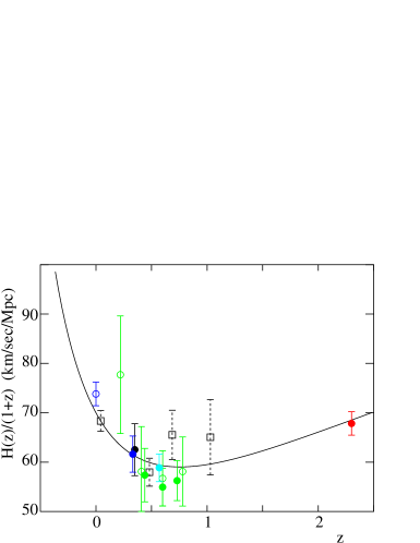
Figure 1: Observational data on the time derivative of the scale factor as function of redshift $z$ [5]. The change of the behavior from decreasing to increasing, as $z$ decreases, means the change from decelerated to accelerated expansion. The theoretical curve corresponds to spatially flat Universe with $h=0.7$ and $\Omega_{\Lambda}=0.73$.

In the case of the cosmological constant, energy-momentum tensor is proportional to metric, and in locally-Lorentz frame it reads

$$T_{\mu\nu}=\rho_{\Lambda}\eta_{\mu\nu}\;,$$

where $\eta_{\mu\nu}$ is the Minkowski tensor. Hence $w_{\Lambda}=-1$. One can view this as the characteristic of vacuum, whose energy-momentum tensor must be Lorentz-covariant. As we pointed out above, any deviation from $w=-1$ would mean that we are dealing with something other than vacuum energy density.

The problem with dark energy is that its present value is extremely small by particle physics standards,

$$\rho_{DE}\approx 4~{}\mbox{GeV/m${}^{3}$}=(2\times 10^{-3}\mbox{eV})^{4}\,.$$

In fact, there are two hard problems. One is that the dark energy density is zero to an excellent approximation. Another is that it is non-zero nevertheless, and one has to understand its energy scale. We are not going to discuss these points anymore, and only emphasize that we are not aware of a compelling mechanism that solves any of the two cosmological constant problems (with possible exception of anthropic argument due to Weinberg and Linde [6, 7]).

3 Cornerstones of thermal history

3.1 Recombination = photon last scattering

Going back in time, we reach so high temperatures that the usual matter (electrons and protons with rather small admixture of light nulei, mainly ⁴He) is in the plasma phase. In plasma, photons interact with electrons due to the Thomson scattering and protons have Coulomb interaction with electrons. These interactions are strong enough to keep photons, electrons and protons in thermal equilibrium. When the temperature drops to

$$T_{rec}\approx 3000~{}{\mbox{K}}\;,\;\;\;\;\;\;z_{rec}\approx 1090\;,$$

almost all electrons “recombine” with protons into neutral hydrogen atoms (helium recombined earlier). The number density of atoms at that time is quite small, $250~{}\mbox{cm}^{-3}$, so from that time on, the Universe is transparent to photons. Thus, $T_{rec}$ is photon last scattering temperature. At that time the age of the Universe is $t_{rec}\approx 380$ thousand years (for comparison, its present age is about 13.8 billion years).

CMB photons give us (literally!) the photographic picture of the Universe at photon last scattering epoch. The last scattering epoch lasted considerably shorter than the then Hubble time $H^{-1}(t_{rec})\sim t_{rec}$; to a meaningful (although rather crude) approximation, recombination occured instantaneously. This is important, since in the opposite case of long recombination, the photographic picture would be strongly washed out.

This photographic picture is shown in Fig. 2. Here brighter (darker) regions correspond to higher (lower) temperatures. The relative temperature fluctuation is of order $\delta T/T=10^{-4}-10^{-5}$, so the 380 thousand year old Universe was much more homogeneous than today.

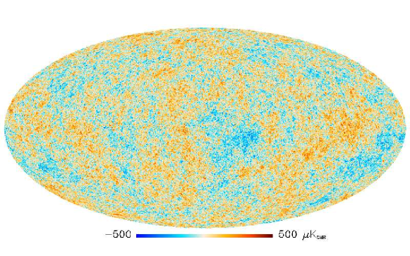
Figure 2: CMB sky as seen by Planck.

One performs Fourier decomposition of the temperatue fluctuations, i.e., decomposition in spherical harmonics:

$$\frac{\delta T}{T}(\theta,\varphi)=\sum_{l,m}a_{lm}Y_{lm}(\theta,\varphi)\;.$$

Here $a_{lm}$ are independent Gaussian random variables (no non-Gaussianities have been found so far) with $\langle a_{lm}a^{*}_{l^{\prime}m^{\prime}}\rangle\propto\delta_{ll^{\prime}}\delta_{mm^{\prime}}$ and $\langle a^{*}_{lm}a_{lm}\rangle=C_{l}$. The multipoles $C_{l}$, or, equivalently,

$$D_{l}=\frac{l(l+1)}{2\pi}C_{l}$$

are the main quantities of interest. The larger $l$, the smaller angular scales, hence the shorter wavelengths of density perturbations producing the temperature anisotropy.

It is worth noting that averaging here is understood in terms of an ensemble of Universes, while we have just one Universe. So, there is inevitable uncertainty in $C_{l}$, called cosmic variance. For given $l$, one has $(2l+1)$ quantities $a_{lm}$, $m=0,\pm 1,\dots,\pm l$, so the uncertainty is $\Delta C_{l}/C_{l}\simeq 1/{\sqrt{2l}}$.

CMB temperature multipoles are shown in Fig. 3 (error bars there are due to cosmic variance, not the measurement errors). Also measured are CMB polarization multipoles and temperature-polarization cross-correlation multipoles. There is a lot of physics behind these quantities, which has to do with

• primordial perturbations: the perturbations that are built in already at the beginning of the hot cosmological epoch, see Sec. 11;

• development of sound waves in cosmic plasma from the early hot stage to recombination; gravitational potentials due to dark matter at recombination (which are sensitive to the composition of cosmic medium);

• propagation of photons after recombination (which is sensitive to expansion history of the Universe and structure formation).

Clearly, CMB measurements are a major source of the cosmological information. We come back to CMB in due course.

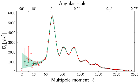
Figure 3: Multipoles $D_{l}$ as measured by Planck.

3.2 Big Bang Nucleosynthesis

As we go back in time further, we get to the temerature in the Universe in MeV range. The epoch characterized by temperatures 1 MeV — 30 keV is the epoch of Big Bang Nucleosynthesis. That epoch starts at temperature 1 MeV, when the age of the Universe is 1 s. At temperatures above 1 MeV, there are rapid weak processes like

$$e^{-}+p\longleftrightarrow n+\nu_{e}\;.$$ (26)

These processes keep neutrons and protons in chemical equilibrium; the ratio of their number densities is determined by the Boltzmann factor, $n_{n}/n_{p}=\mbox{exp}\left(-\frac{m_{n}-m_{p}}{T}\right)$. At $T_{n}\approx 1$ MeV neutron-proton transitions (26) switch off, and neutron-proton ratio is frozen out at the value

$$\frac{n_{e}}{n_{p}}={\rm e}^{-\frac{m_{n}-m_{p}}{T_{n}}}\;.$$

Interestingly, $m_{n}-m_{p}\sim T_{n}$, so the neutron-proton ratio at neutron freeze-out and later was neither equal to 1, nor very small. Were it equal to 1, protons would in the end combine with neutrons into ⁴He, and there would remain no hydrogen in the Universe. On the other hand, for very small $n_{n}/n_{p}$, too few light nuclei would be formed, and we would not have any observable remnants of the BBN epoch. In either case the Universe would be quite different from what it actually is. It is worth noting that the approximate relation $m_{n}-m_{p}\sim T_{n}$ is a coincidence: $m_{n}-m_{p}$ is determined by light quark masses and electromagnetic coupling, while $T_{n}$ is determined by the strength of weak interactions (the rates of the processes (26)) and gravity (the expansion of the Universe). This is one of numerous coincidences we encounter in cosmology.

At temperatures 100 – 30 keV, neutrons combined with protons into light elements in thermonuclear reactions

$$p+n \to {}^{2}\mbox{H}+\gamma\;,$$

$${}^{2}\mbox{ H}+p \to {}^{3}\mbox{ He}+\gamma\;,$$

$${}^{3}\mbox{He}+^{2}\mbox{H} \to {}^{4}\mbox{ He}+p\;,$$ (27)

etc., up to ⁷Li. The abundances of light elements have been measured, see Fig. 4. The only parameter relevant for calculating these abundances (assuming negligible neutrino-antineutrino asymmetry) is the baryon-to-photon ratio $\eta_{B}\equiv\eta$, see eq. (23), which determines the number density of baryons. Comparison of the Big Bang Nucleosynthesis theory with the observational determination of the composition of cosmic medium enables one to determine $\eta_{B}$ and check the overall consistency of the BBN picture. It is even more reassuring that a completely independent measurement of $\eta_{B}$ that makes use of the CMB temperature fluctuations is in excellent agreement with BBN. Thus, BBN gives us confidence that we understand the Universe at $T\sim 1$ MeV, $t\sim 1$ s. In particular, we are convinced that the cosmological expansion was governed by General Relativity.

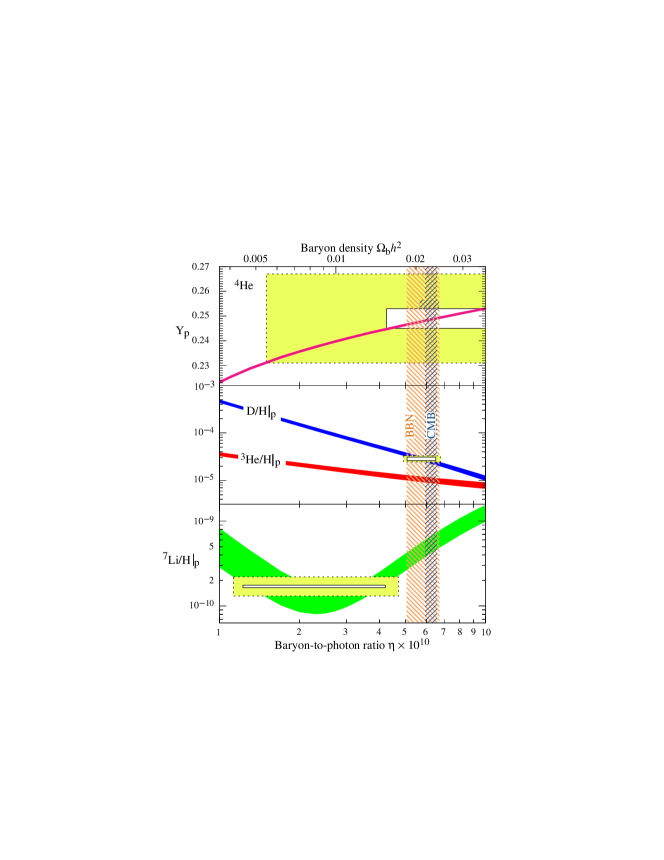
Figure 4: Abundances of light elements, measured (boxes; larger boxes include systematic uncertainties) and calculated as functions of baryon-to-photon ratio $\eta$ [8]. The determination of $\eta\equiv\eta_{B}$ from BBN (vertical range marked BBN) is in excellent agreement with the determination from the analysis of CMB temperature fluctiations (vertical range marked CMB).

3.3 Neutrino decoupling

Another class of processes of interest at temperatures in the MeV range is neutrino production, annihilation and scattering,

$$\nu_{\alpha}+\bar{\nu}_{\alpha}\longleftrightarrow e^{+}+e^{-}$$

and crossing processes. Here the subscript $\alpha$ labels neutrino flavors. These processes switch off at $T\sim 2-3$ MeV, depending on neutrino flavor. Since then neutrinos do not interact with cosmic medium other than gravitationally, but they do affect the properties of CMB and distribution of galaxies through their gravitational interactions. Thus, observational data can be used to establish, albeit somewhat indirectly, the existence of relic neutrinos and set limits on neutrino masses. We quote here the limit reported by Planck collaboration [3]

$$\sum m_{\nu}<0.12~{}\mbox{eV}\;,$$

where the sum runs over the three neutrino species. Other analyses give somewhat weaker limits. Also, the data can be used to determine the effective number of neutrino species that counts the number of relativistic degrees of freedom [3]:

$$N_{\nu,\,eff}=2.99\pm 0.17\;,$$

which is consistent with the Standard Model value $N_{\nu}=3$. We see that cosmology requires relic neutrinos.

4 Dark matter: evidence

Unlike dark energy, dark matter experiences the same gravitational force as the baryonic matter. Dark matter is discussed in numerous reviews, see, e.g., Refs. [9, 10, 11, 12]. It consists presumably of new stable massive particles. These make clumps of mass which constitute most of the mass of galaxies and clusters of galaxies. Dark matter is characterized by the mass-to-entropy ratio,

$$\left(\frac{\rho_{DM}}{s}\right)_{0}=\frac{\Omega_{DM}\rho_{c}}{s_{0}}\approx\frac{0.26\cdot 5\cdot 10^{-6}~{}\mbox{GeV}\cdot\mbox{cm}^{-3}}{3000~{}\mbox{cm}^{-3}}=4\cdot 10^{-10}~{}\mbox{GeV}\;.$$ (28)

This ratio is constant in time since the freeze out of dark matter density: both number density of dark matter particles $n_{DM}$ (and hence their mass density $\rho_{DM}=m_{DM}n_{DM}$) and entropy density decrease exactly as $a^{-3}$.

There are various ways of measuring the contribution of non-baryonic dark matter into the total energy density of various objects and the Universe as a whole.

4.1 Dark matter in galaxies

Dark matter exis in galaxies. Its distribution is measured by the observations of rotation velocities of distant stars and gas clouds around a galaxy, Fig. 5. If the mass was concentrated in a luminous central part of a galaxy, the velocities of objects away from the central part would decrease with the distance $r$ to the center as $v\propto r^{-1/2}$ – this immediately follows from the second Newton’s law

$$\frac{v^{2}}{r}=G\frac{M(r)}{r^{2}}\;.$$

In reality, rotation curves are typically flat up to distances exceeding the size of the bright part by a factor of 10 or so. The fact that dark matter halos are so large is explained by the defining property of dark matter particles: they do not lose their energies by emitting photons, and, in general, interact with conventional matter very weakly.

Figure 5: Rotation velocities of hydrogen gas clouds around a galaxy NGC 6503 [13]. Lines show the contributions of the three main components that produce the gravitational potential. The main contribution at large distances is due to dark matter, labeled “halo”.

4.2 Dark matter in clusters of galaxies

Dark matter makes most of the mass of the largest gravitationally bound objects – clusters of galaxies. There are various methods to determine the gravitating mass of a cluster, and mass distribution in a cluster, which give consistent results. These include measurements of rotational velocities of galaxies in a cluster (original Zwicky argument that goes back to 1930’s), measurements of temperature of hot gas (which actually makes most of baryonic matter in clusters), observations of gravitational lensing of extended light sources (galaxies) behind the cluster, see Fig. 6. All these determinations show that baryons (independently measured through their X-ray emission) make less than 1/4 of total mass in clusters. The rest is dark matter.

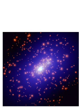
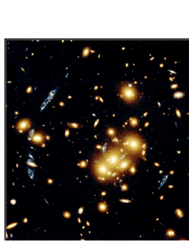
Figure 6: Cluster of galaxies CL$0024+1654$ [14], acting as gravitational lens. Right panel: cluster in visible light. Round yellow spots are galaxies in the cluster. Elongated blue strips are images of one and the same galaxy behind the cluster. Left panel: reconstructed distribution of gravitating mass in the cluster; brighter regions have larger mass density.

Concerning galaxies and clusters of galaxies, we note that there are attempts to attribute the properties of rotation curves and other phenomena, which are usually considered as evidence for dark matter, to modification of gravity, and in this way get rid of dark matter altogether. There are several strong arguments that rule out this idea. One argument has to do with the Bullet Cluster, Fig. 7. Shown are two galaxy clusters that passed through each other. The dark matter and galaxies do not experience friction and thus do not lose their velocities. On the contrary baryons in hot, X-ray emitting gas do experience friction and hence get slowed down and lag behind dark matter and galaxies. In this way the baryons (which are mainly in hot gas) and dark matter are separated in space. Since the baryonic mass and gravitational potentials are not concentric, one cannot attribute gravitational potentials solely to baryons, even assuming the modification of Newton’s gravity law. As a remark, the fact that dark matter moves after cluster collision considerably faster than baryonic gas means that elastic scattering between dark matter particles is weak. Quantitatively, the limit on the dark matter elastic scattering cross section is

$$\sigma^{(el)}_{DM-DM}<1\cdot 10^{-24}~{}\mbox{cm}^{2}\;.$$ (29)

This limit is not particularly strong, but it does rule out part of the parameter space of strongly interacting massive particle (SIMP) dark matter models, see Sec. 5.2.

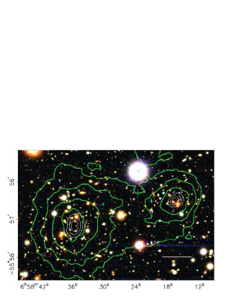
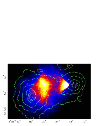
Figure 7: Observation [15] of the Bulet Cluster 1E0657–558 at $z=0.296$. Closed lines show the gravitational potential produced mainly by dark matter and measured through gravitational lensing. Bright regions in the right panel show X-ray emission of hot baryon gas, which makes most of the baryonic matter in the clusters. The length of white interval is 200 kpc in comoving frame.

4.3 Dark matter imprint in CMB

Composition of the Universe strongly affects the CMB angular anisotropy and polarization. Before recombination, the energy density perturbation is a sum of perturbation in baryon-electron-photon component and dark matter component,

$$\delta\rho=\delta\rho_{B}+\delta\rho_{DM}$$

(we simplify things here, as there is also perturbation in gravitational potentials induced by density perturbation). The tightly coupled baryon-electron-photon plasma has high pressure (due to photon component with $p_{\gamma}=\rho_{\gamma}/3$), so density perturbations in this fraction undergo acoustic oscillations: every Fourier mode oscillates in time as

$$\delta\rho_{B}({\bf k},t)=A({\bf k})\mbox{cos}\left(\int_{0}^{t}v_{s}\frac{k}{a(t)}dt\right)\;,$$ (30)

where ${\bf k}$ is comoving momentum (and ${\bf k}/a(t)$ is physical momentum which gets redshifted), $v_{s}\approx 1/\sqrt{3}$ is sound speed, and $A({\bf k})$ is the amplitude that varies slowly with $k$ (in statistical sense: $\delta\rho({\bf k})$ is Gaussian random field). We comment in Sec. 11 on the fact that the phase of cosine in (30) is well defined. On the contrary, dark matter is pressureless, so its perturbation is almost independent of time,

$$\delta\rho_{DM}\approx\delta\rho_{DM}({\bf k})\;,$$

where $\delta\rho_{DM}({\bf k})$ slowly varies with $k$. At recombination time $t_{r}$, the energy density perturbation is a sum

$$\delta\rho({\bf k},t_{r})=A({\bf k})\mbox{cos}\left(\int_{0}^{t_{r}}v_{s}\frac{k}{a(t)}dt\right)+\delta\rho_{DM}({\bf k})\;.$$ (31)

The first term here oscillates as function of $k$, while the second term is a smooth, non-oscillating function of $k$.

Now, behavior of $\delta\rho(t_{r})$ as function of spatial momentum $k$ translates into behavior of CMB temperature fluctuation $\delta T$ as function of multipole number $l$. $\delta T$ at a given point in space at recombination epoch is proportional to $\delta\rho$ (here we again simplify things, this time quite considerably). We see CMB coming from a photon last scattering sphere; smaller angular scale in this photographic picture corresponds to smaller spatial scale at recombination epoch, hence larger multipole $l$ corresponds to higher three-momentum $k$. Thus, oscillatory formula (31) translates into oscillatory behavior in Fig. 3. Both oscillatory part of temperature angular spectrum (which is due to the first, baryonic term in (31)) and smooth part (due to the second, dark matter term in (31)) are clearly visible in Fig. 3. The detailed analysis of this angular spectrum enables one to determine both baryon content and dark matter content in the Universe, $\Omega_{B}$ and $\Omega_{DM}$ quoted in (10).

4.4 Dark matter and structure formation

Dark matter is crucial for our existence, for the following reason. As we discussed above, density perturbations in baryon-electron-photon plasma before recombination do not grow because of high pressure; instead, they oscillate with time-independent amplitudes. Hence, in a Universe without dark matter, density perturbations in baryonic component would start to grow only after baryons decouple from photons, i.e., after recombination. The mechanism of the growth is qualitatively simple: an overdense region gravitationally attracts surrounding matter; this matter falls into the overdense region, and the density contrast increases. In the expanding, matter dominated Universe this gravitational instability results in the density contrast growing like $(\delta\rho/\rho)(t)\propto a(t)$. Hence, in a Universe without dark matter, the growth factor for baryon density perturbations would be at most

$$\frac{a(t_{0})}{a(t_{rec})}=1+z_{rec}=\frac{T_{rec}}{T_{0}}\approx 10^{3}\;.$$ (32)

The initial amplitude of density perturbations is very well known from the CMB anisotropy measurements, $(\delta\rho/\rho)_{i}=5\cdot 10^{-5}$. Hence, a Universe without dark matter would still be nearly homogeneous: the density contrast would be in the range of a few per cent. No structure would have been formed, no galaxies, no life. No structure would be formed in future either, as the accelerated expansion due to dark energy will soon terminate the growth of perturbations.

Since dark matter particles decoupled from plasma much earlier than baryons, perturbations in dark matter started to grow much earlier. The corresponding growth factor is larger than (32), so that the dark matter density contrast at galactic and sub-galactic scales becomes of order one, perturbations enter non-linear regime, collapse and form dense dark matter clumps at $z=5~{}-~{}10$. Baryons fall into potential wells formed by dark matter, so dark matter and baryon perturbations work together soon after recombination. Galaxies get formed in the regions where dark matter was overdense originally. For this picture to hold, dark matter particles must be non-relativistic early enough, as relativistic particles fly through gravitational wells instead of being trapped there. This means, in particular, that neutrinos cannot constitute a considerable part of dark matter.

4.5 Digression. Standard ruler: BAO

Before recombination, the sound speed in baryon-electron-photon component is about $v_{s}\approx 1/\sqrt{3}$. After recombination, baryons (atoms) decouple from photons, sound speed in baryon component is practically zero, and baryons no longer move in space. This leads to a feature in the spatial distribution of matter (galaxies) which is known as Baryon Acoustic Oscillations (BAO). It is worth noting that similar phenomenon was described by A.D. Sakharov [16] back in 1965, but in the context of cold cosmological model (Sakharov’s paper was written before the discovery of CMB).

Phyiscs behind BAO is illustrated in Fig. 8. Suppose there is an overdense region in the very early Universe (in the beginning of the hot epoch). Importantly, the initial conditions for baryon-electron-photon component and dark matter are the same: overdensity exists in both of them in the same place in space (this is the property of adiabatic scalar perturbations; CMB measurements ensure that primordial perturbations are indeed adiabatic). This initial condition is shown in the left panel of Fig. 8. Before recombination, dark matter perturbation stays in the same place, while perturbation in baryon-electron-photon component moves away with the sound speed. If the initial perurbarion is spherically symmetric, then the sound wave is spherical, as shown in the right panel. At recombination, the baryon perturbation is frozen in, and the whole picture expands merely due to the cosmological expansion. The comoving distance between the dark matter overdensity and baryon overdensity shell is the comoving sound horizon at recombination

$$r_{s}=\int_{0}^{t_{r}}v_{s}\frac{k}{a(t)}dt$$

(this is precisely the argument of cosine in (31)); its present value is $r_{s}\simeq 150$ Mpc (we set $a_{0}=1$ here), and the value at redshift $z$ is $r_{s}/(1+z)$.

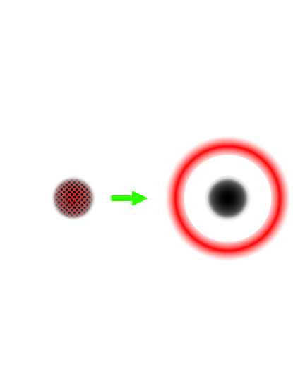
Figure 8: Schematic picture of Baryon Acoustic Oscillations. Dark regions show dark matter overdensity, less dark (red) regions are the ones with baryon overdensity. Left: initial condition. Right: at recombination and later.

Due to BAO, there is correlation between the matter densities (dark matter plus baryons) separated by comoving distance $r_{s}$. It shows up as a feature in the galaxy-galaxy correlation function $\xi(s)$, where $s$ is comoving distance. This bump in the correlation function was detected in Ref. [17], see Fig. 9. Clearly, BAO serves as a standard ruler at various redshifts, which can be used to study the evolution of the Universe in not so distant past.

Currently, BAO is a very powerful tool of observational cosmology. It is used, in particular, to study time (in)dependence of dark energy.

The bump in the spatial correlation function translates into oscillations in momentum space, hence the name.

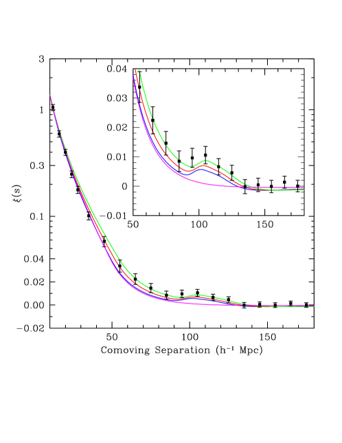
Figure 9: The first detection of BAO: the correlation function $\xi\left(s\right)$ determined by the analysis of the SDSS data on the distribution of distant galaxies. Solid lines show the predictions of various cosmological models. Green, red and blue lines correspond to $\Omega_{M}h^{2}=0.12,0.13,0.14$, respectively, with $\Omega_{B}h^{2}=0.024$, $n_{s}=0.98$ in all cases. Magenta line corresponds to unrealistic Universe without baryons. The parameter $h$ is defined in (4); numerically, $h_{0}\approx 0.7$.

5 Astrophysics: more hints on dark matter properties

Important information on dark matter properties is obtained by theoretical analysis of structure formation and its comparison with observational data. Indeed, as we discussed above, dark mater plays the key role in structure formation, so properties of galaxies and their distribution in space potentially tell us a lot about dark matter.

Currently, theoretical studies are made mostly via numerical simulations, many of which ignore effects due to baryons (dark-matter-only). Thus, these simulations give the dark matter distribution. To compare it with observed structures, one often assumes that baryons trace dark matter, with qualification that baryons are capable of losing their kinetic energy and forming more compact structures inside dark matter halos. In other words, simulated dark matter collapsed clump of a mass charactersitic of a galaxy is associated with a visible galaxy, heavier dark matter clumps are interpreted as clusters of galaxies, etc.

Currently, the most popular dark matter scenario is cold dark matter, CDM. It consists of particles whose velocities are negligible at all stages of structure formation, and whose non-gravitational interactions with themselves and with baryons are negligible too (from the viewpoint of structure formation). The CDM numerical simulations (plus the above assumption concerning baryons) are in very good agreement with observations at relatively large spatial scales. This is an important result that implies interesting limits on dark matter properties, which we discuss below.

However, there are astrophysical phenomena at shorter scales that may or may not hint towards something different from weakly interacting CDM. The situation is inconclusive yet, but it is worth keeping in mind these phenomena, which we now discuss in turn.

5.1 Missing satellite problem: astrophysics vs warm dark matter

It has long been known that CDM-only simulations produce a lot of small mass halos, $M\lesssim 10^{9}M_{\odot}$ where $M_{\odot}$ is the Solar mass. Galaxies like Milky Way have masses $(10^{11}-10^{12})M_{\odot}$, so we are talking about dwarf galaxies. As an example, the left panel of Fig. 10 shows the simulated dark matter distribution in a ball of radius 250 kpc around a galaxy similar to Milky Way. Assuming that baryons trace dark matter, one observes that there must be hundreds of satellite galaxies there. The actual Milky Way satellites are shown in the right panel of Fig. 10; clearly the number of satellites is a lot smaller. This is the missing satellite problem.

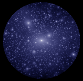
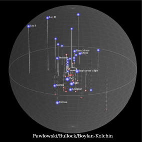
Figure 10: Left: CDM-only simulation of 250 kpc vicinity of a galaxy like Milky Way; right: actual distribution of satellite galaxies in 250 kpc vicinity of Milky Way [12].

It is conceivable that this problem has astrophysical solution within CDM model. One point is that the number of observed faint satellite galaxies around Milky Way is not that small any longer: while a few years ago this number was about 20, it is currently about 60, and this is not a comlete sample because of limited detection efficiency – the expectation [18] for a complete sample is 150 – 300 with masses exceeding $10^{8}M_{\odot}$. Another property is that dark matter halos of mass $M<10^{9}M_{\odot}$ appear fairly inefficient in forming luminous component — this has been suggested by simulations that include numerous effects due to baryons [19, 20]. Thus, if CDM model is correct, and missing satellite problem has astrophysical solution, there must be a large number of ultra-faint dwarf galaxies with masses $(10^{8}-10^{9})M_{\odot}$ and even larger number of non-luminous dark matter halos with $M\lesssim 10^{8}M_{\odot}$ in the vicinity of Milky Way. This prediction will be possible to check in near future, notably, with Large Synoptic Survey Telescope, LSST [22].

An alternative, particle physics solution to the missing satellite problem is warm dark matter, WDM. A reasonably well motivated WDM candidate is sterile neutrino, which we discuss in Sec. 8. Another popular candidate is light gravitino. In WDM case, dark matter particles decouple from kinteic equilibrium with baryon-photon component when they are relativistic. Let us assume for definiteness that they are in kinetic equilibrium with cosmic plasma at temperature $T_{f}$ when their number density freezes out (there is no chemical equilibrium at $T=T_{f}$, otherwise the dark matter would be overabundant). After kinetic equilibrium breaks down at temperature $T_{d}\leq T_{f}$, the spatial momenta decrease as $a^{-1}$, i.e., the momenta are of order $T$ all the time after decoupling. When dark matter particles are relativistic, the density perturbations do not grow: relativistic particles escape from the gravitational potentials, so they do not experience the gravitational instability; in fact, the density perturbations, and hence the gravitational wells get smeared out instead of getting deeper. WDM particles become non-relativistic at $T\sim m$, where $m$ is their mass. Only after that the WDM perturbations start to grow. Before becoming non-relativistic, WDM particles travel the distance of the order of the horizon size; the WDM perturbations therefore are suppressed at those scales. The horizon size at the time $t_{nr}$ when $T\sim m$ is of order

$$l_{H}(t_{nr})\simeq H^{-1}(T\sim m)=\frac{M_{Pl}^{*}}{T^{2}}\sim\frac{M_{Pl}^{*}}{m^{2}}\;.$$

Due to the expansion of the Universe, the corresponding length at present is

$$l_{0}=l_{H}(t_{nr})\frac{a_{0}}{a(t_{nr})}\sim l_{H}(t_{nr})\frac{T}{T_{0}}\sim\frac{M_{Pl}}{mT_{0}}\;,$$ (33)

where we neglected (rather weak) dependence on $g_{*}$. Hence, in WDM scenario, structures of comoving sizes smaller than $l_{0}$ are less abundant as compared to CDM. Let us point out that $l_{0}$ refers to the size of the perturbation in the linear regime; in other words, this is the size of the region from which matter collapses into a compact object.

To solve the missing satellite problem, one requires that the mass of dark matter which was originally distributed over the volume of comoving size $l_{0}$, and collapsed later on, is of order of the mass of satellite galaxy,

$$\frac{4\pi}{3}l_{0}^{3}\Omega_{DM}\rho_{c}\sim M_{dwarf}\;.$$

With $M_{dwarf}\sim 10^{8}M_{\odot}$ we find $l_{0}\sim 100$ kpc, and eq. (33) gives the estimate for the mass of a dark matter particle

$$\mbox{WDM}\;:\;\;\;\;m_{DM}=3~{}-~{}10~{}\mbox{keV}\;.$$ (34)

On the other hand, this effect is absent, i.e., dark matter is cold, for

$$\mbox{CDM}\;:\;\;\;\;m_{DM}\gtrsim 10~{}\mbox{keV}\;.$$ (35)

Let us recall that these estimates apply to particles that are initially in kinetic equilibrium with cosmic plasma. They do not apply in the opposite case; an example is axion dark matter, which is cold despite of very small axion mass.

Reversing the argument, one obtains a limit on the mass of WDM particle which decouples in kinetic equilibtium [18],

$$m\gtrsim 4~{}\mbox{keV}\;.$$ (36)

5.1.1 Digression: phase space bound

In fact there are other ways to obtain the limits on $m$. One has to do with phase space density: the maximum value of coarse grained phase space density

$$f(p,x)_{coarse~{}grained}=\left(\frac{dN}{d^{3}p\,d^{3}x}\right)_{coarse~{}grained}$$

does not decrease in the course of the evolution (here $N$ is the number of particles). Indeed, Liouville theorem tells that the microscopic phase space density is time-independent. What happens in the course of evolution is that particles penetrate initially unoccupied regions of phase space, see Fig. 11. While the maximum value of the microscopic phase space density remains constant in time, the maximum value of coarse grained phase space density (average over phase space volume shown by dashed line in Fig. 11) decreases.

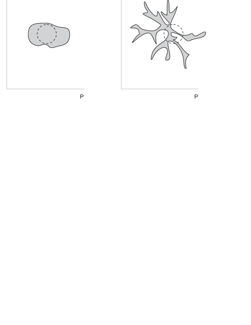
Figure 11: Sketch of the behavior of an ensemble of particles in phase space. As the ensemble evolves, initial compact distribution (left panel) becomes less compact.

The initial phase space density of particles in kinetic equilibrium is

$$f_{i}=\frac{A}{(2\pi)^{3}}\frac{1}{\mbox{e}^{p/T}+1}\;,$$

where we consider fermions for definiteness. The parameter $A$ is determined by requiring that the number density $n$ takes prescribed value, so that

$$n_{0}=\frac{\Omega_{DM}\rho_{c}}{m}\;.$$

We find

$$n=\int f_{i}d^{3}p=A\cdot\frac{3\zeta(3)}{4\pi^{2}}T^{3}\;,$$

where $\zeta(3)\approx 1.2$. So, the maximum of the initial phase space density is

$$f_{i,\,max}=\frac{n}{12\pi\zeta(3)T^{3}}=\frac{\Omega_{DM}\rho_{c}}{12\pi\zeta(3)mT_{0\,eff}^{3}}\;,$$

where $T_{0\,eff}$ depends on the decoupling temperature and is somewhat lower than the present photon temperature.

On the other hand, one can measure a quantity

$$Q=\frac{\rho_{DM,\,gal}}{\langle v_{gal}^{2}/3\rangle^{3/2}}$$

where $\rho_{DM,\,gal}$ is mass density (say, in a central part of dwarf galaxy), $\langle v_{gal}^{2}\rangle$ is average velocity squared, and hence $\langle v_{gal}^{2}/3\rangle$ is the average velocity squared along the line of sight (of stars, and hence dark matter particles, in a virialized galaxy). Since $v_{gal}=p_{gal}/m$ and $\rho_{DM,\,gal}=mn_{gal}$, one obtains an estimate for the phase space density of dark matter particles in a dwarf galaxy,

$$f\simeq\frac{n_{gal}}{\langle p_{gal}^{2}\rangle^{3/2}}=\frac{Q}{3^{3/2}m^{4}}\;.$$

One requires that

$$f<f_{i\,max}$$

and obtains the bound on the mass of the dark matter particle

$$m\gtrsim 3\cdot\left(\frac{Q}{\Omega_{DM}\rho_{c}}\right)^{1/3}T_{0\,eff}\;.$$

The values of $Q$ measured in compact dwarf galaxies are in the range

$$Q\sim(5\cdot 10^{-3}-2\cdot 10^{-2})\cdot\frac{M_{\odot}/\mbox{pc}^{3}}{(km/s)^{3}}$$

while for relic that decouples at $T=(1-100)~{}\mbox{MeV}$ one has $T_{0\,eff}=2.0~{}\mbox{K}$. This gives [23, 24]

$$m\gtrsim 6~{}\mbox{keV}\;.$$

Accidentally, this bound is similar to (36). We note that bounds coming from phase space density considerations are called bounds of Tremain–Gunn type.

We also note that similar (in fact, slightly stronger but less robust) bounds are obtained by the study of Lyman-$\alpha$ forest, see, e.g., Ref [25].

5.2 Other hints, SIMP and fuzzy DM

There are two other issues that may or may not be problematic for CDM. One is the “core-cusp problem”: CDM-only simulations show singular mass density profiles (cusps) in the centers of galaxies, $\rho_{DM}(r)\propto r^{-1}$, while observations imply enhanced but smooth profiles (cores). Another is “too-big-to-fail” problem, which currently means that the densities in large satellite galaxies ($M\sim 10^{10}~{}M_{\odot}$), predicted by CDM-only simulations, are systematically higher than the observed mass densities [12].

The astropysical solutions to these problems again have to do with baryons (supernovae feedback, etc.), and also interactions of satellite galaxies with large host galaxy, Milky Way, see, e.g., Refs. [12, 26] for discussion. On the particle physics side, WDM may again help out. Two other particle physics solutions are Strongly Intracting Massive Particles (SIMP) as dark matter, and fuzzy dark matter.

The idea of SIMP [27] is that dark matter is cold, but elastic scattering of dark matter particles smoothes out the cuspy mass distribution in galactic centers. Elastic scattering can also lead to decrease of the dark matter density and thus alleviate the too-big-to-fail problem. To give an idea of the elastic scattering cross section, we take mass density of dark matter of order $\rho_{DM}\sim 1~{}\mbox{GeV}/\mbox{cm}^{3}$ and require that the mean free path of dark matter particle is of order $l\sim 1$ kpc (typical values, by order of magnitude, both for centers of large galaxies and for dwarf galaxies),

$$1\sim l\sigma^{(el)}n_{DM}=l\sigma^{(el)}\frac{\rho_{DM}}{m}\;,$$

and obtain

$$\frac{\sigma^{(el)}}{m}\sim\frac{1}{l\rho_{DM}}\sim 10^{-24}\frac{\mbox{cm}^{2}}{\mbox{GeV}}\;.$$

This is a very large cross section by particle physics standards, and, in view of (29), dark matter particle must be fairly light, $m\lesssim 1$ GeV. The large elastic cross section may be due to $t$-channel exchange of light mediator with $m_{med}\sim 10-100$ MeV. This mediator must decay into $e^{+}e^{-}$, $\gamma\gamma$, etc., otherwise it would be dark matter itself. All these features make SIMP scenario interesting from the viewpoint of collider (search in $Z$-decays) and “beyond collider” experiments, such as SHiP.

Yet another proposal is fuzzy dark matter consisting of very light bosons,

$$m\sim(10^{-21}-10^{-22})~{}\mbox{eV}\;.$$

The mechanism of their production must ensure that all of them are born with zero momenta, i.e., these particles form scalar condensate. An oversimplified picture is that the de Broglie wavelength of these particles at velocities typical for galactic centers and dwarf galaxies, $v\sim 10~{}\mbox{km}/\mbox{s}$, is about 1 kpc:

$$\frac{2\pi}{mv}\sim 1~{}\mbox{kpc}\;.$$

Detailed discussion of advantages of fuzzy dark matter is given, e.g., in Ref. [28]. A way to constrain this scenatio is again to study Lyman-$\alpha$ forest; current constraints [29] are at the level $2\cdot 10^{-21}$ eV. Interestingly, effects of fuzzy dark matter may in future be detected by pulsar timing method [30].

From particle physics viewpoint, fuzzy dark matter particles may emerge as pseudo-Nambu–Goldstone bosons, similar to axions. We discuss axions later, and here we borrow the main ideas. The axion-like Lagrangian for the pseudo-Nambu–Goldstone scalar field $\theta$ reads

$$L=\frac{F^{2}}{2}(\partial\theta)^{2}-{\mu^{4}}(1-\cos^{2}\theta)\approx\frac{F^{2}}{2}(\partial\theta)^{2}-\frac{\mu^{4}}{2}\theta^{2}\;,$$

where $F$ is the expectation value of a field that spontaneously breaks approximate $U(1)$ symmetry, and $\mu$ is the parameter of the explicit violation of this symmetry. Then the mass of the axion-like particle is

$$m=\frac{\mu^{2}}{F}\;.$$

The mechanism that creates the scalar condensate is misalignment. The initial value of $\theta$ is an arbitrary number between $-\pi$ and $\pi$, so that $\theta_{i}\sim 1$. The field starts to oscillate when the expansion rate becomes small enough, $H\sim m$. The calculation of the present mass density is a simplified version of the axion calculation that we give in Sec. 7; one finds that $\Omega_{DM}\sim 0.25$ is obtained for $m=10^{-22}$ eV if

$$F\sim 10^{17}~{}\mbox{GeV}\;.$$

This is in the ballpark of GUT/string scales, which is intriguing.

5.3 Summary of DM astrophysics

Let us summarize the astrophysics of dark matter.

• Cold dark matter descibes remarkably well the distrubution and properties of structures in the Universe at relatively large scales, from galaxies like Milky Way or somewhat smaller ($M\gtrsim 10^{11}M_{\odot}$) to larger structures like clusters of galaxies, filaments, etc.; also, CDM is remarkably consistent with CMB data which probe even larger scales.

• Currently, data and simulations at shorter scales are inconclusive: they may or may not show that there are “anomalies”, the features that contradict CDM model.

• It will become clear fairly soon whether these “anomalies” are real or not. The progress will come from refined simulations with all effects of baryons included, and from new instruments, notably LSST.

• If the “anomalies” are real, we will have to give up CDM, and, responding to the data, will narrow down the set of dark matter models (WDM, or SIMP, or fuzzy dark matter, or something else). This will have a profound effect on the strategy of search for dark matter particles.

• If the “anomalies” are not there, astrophysics will have to deliver the confirmation of CDM model by the discoveries of relatively light ultra-faint dwarf galaxies ($M=(10^{8}-10^{9})M_{\odot}$) and dark objects of even smaller mass.

All this makes astrophysics a powerful tool of studying dark matter and directing particle physics in its search for dark matter particles.

6 Thermal WIMP

6.1 WIMP abundance: annihilation cross section

Thermal WIMP (weakly interacting massive particle) is a scenario featuring a simple mechanism of the dark matter generation in the early Universe. WIMP is a cold dark matter candidate. Because of its simplicity and robustness, it has been considered by many as the most likely one.

Let us not go into all details of (fairly straightforward) calculation of the thermal WIMP abundance. These details are given in several textbooks, and also presented in proceedings of similar Schools, see, e.g., Ref. [31]. Instead, we give the main assumptions behind this mechanism and describe the main steps of the calculation.

One assumes that there exists a heavy stable neutral particle $\chi$, and that $\chi$-particles can only be destroyed or created in cosmic plasma via their pair-annihilation or creation, with annihilation products being the particles of the Standard Model. We note that there is a version of WIMP model in which particle $\chi$ is not truly neutral, i.e., it does not coincide with its own antiparticle. In that case one assumes that the production and destruction occurs only via $\chi-\bar{\chi}$ annnihilation, and there is no asymmetry between $\chi$ and $\bar{\chi}$ in cosmic plasma, $n_{\chi}=n_{\bar{\chi}}$. The calculation in the $\chi-\bar{\chi}$ model is identical to the case of truly neutral particle, so we consider the latter case only.

One also assumes that the $\chi$-particles are not strongly coupled, but $\chi\chi$-annihilation cross section is sufficiently large, so the $\chi$-particles are in complete thermal equilibrium at high temperatures. The latter assumption is justified in the end of the calculation. The thermal equilibrium means, in particular, that the abundance of $\chi$-particles is given by the standard Bose–Einstein or Fermi–Dirac distribution formula.

The cosmological behaviour of $\chi$-particles is as follows. At high temperatures, $T\gg m_{\chi}$, the number density of $\chi$-particles is high, $n_{\chi}(T)\sim T^{3}$. As the temperature drops below $m_{\chi}$, the equilibrium number density decreases,

$$n^{(eq)}_{\chi}\propto\mbox{e}^{-\frac{m_{\chi}}{T}}\;,$$ (37)

At some “freeze-out” temperature $T_{f}$ the number density becomes so small, that $\chi$-particles can no longer meet each other during the Hubble time, and their annihilation terminates. After that the number density of survived $\chi$-particles decreases as $a^{-3}$, and these relic particles form CDM. The freeze-out temperature $T_{f}$ is obtained by equating the mean free time of $\chi$-particle with respect to annihilation,

$$\tau_{ann}(T_{f})=\left(\sigma_{0}(T_{f})n_{\chi}(T_{f})\right)^{-1}$$

to the Hubble time (see (20))

$$H^{-1}(T_{f})=\frac{M_{Pl}^{*}}{T_{f}^{2}}\;.$$

Here we introduced the weighted annihilation cross section

$$\sigma_{0}(T)=\langle\sigma_{ann}v\rangle_{T}\;,$$

where $v$ is the relative velocity of $\chi$-particles (in the non-relativistic regime relevant here we have $v\ll 1$), and we average over the thermal ensemble.

Thus, freeze-out occurs when

$$\sigma_{0}(T_{f})n_{\chi}(T_{f})=\frac{T_{f}^{2}}{M_{Pl}^{*}}\;.$$

Because of exponential decay of $n_{\chi}^{(eq)}$ with temperature, eq. (37), freeze-out temperature is smaller than the mass by a logarithmic factor only,

$$T_{f}\approx\frac{m_{\chi}}{\mathop{\rm ln}\nolimits(M_{Pl}^{*}m_{\chi}\sigma_{0})}\;.$$ (38)

Note that due to large logarithm, $\chi$-particles are indeed non-relativistic at freeze-out: their velocity squared is of order

$$v^{2}(T_{f})\simeq 0.1\;.$$

At freeze-out, the number density is

$$n_{\chi}(T_{f})=\frac{T_{f}^{2}}{M_{Pl}^{*}\sigma_{0}(T_{f})}\;,$$ (39)

Note that this density is inversely proportional to the annihilation cross section (modulo logarithm). The reason is that for higher annihilation cross section, the creation-annihilation processes are longer in equilibrium, and less $\chi$-particles survive. Up to a numerical factor of order 1, the number-to-entropy ratio at freeze-out is

$$\frac{n_{\chi}}{s}\simeq\frac{1}{g_{*}(T_{f})M_{Pl}^{*}T_{f}\sigma_{0}(T_{f})}\;.$$ (40)

This ratio stays constant until the present time, so the present number density of $\chi$-particles is $n_{\chi,0}=s_{0}\cdot\left(n_{\chi}/s\right)_{freeze-out}$, and the mass-to-entropy ratio is

$$\frac{\rho_{\chi,0}}{s_{0}}=\frac{m_{\chi}n_{\chi,0}}{s_{0}}\simeq\frac{\mathop{\rm ln}\nolimits(M_{Pl}^{*}m_{\chi}\sigma_{0})}{g_{*}(T_{f})M_{Pl}^{*}\sigma_{0}(T_{f})}\simeq\frac{\mathop{\rm ln}\nolimits(M_{Pl}^{*}m_{\chi}\sigma_{0})}{\sqrt{g_{*}(T_{f})}M_{Pl}\sigma_{0}(T_{f})}\;,$$

where we made use of (38). This formula is remarkable. The mass density depends mostly on one parameter, the annihilation cross section $\sigma_{0}$. The dependence on the mass of $\chi$-particle is through the logarithm and through $g_{*}(T_{f})$; it is very mild. Plugging in $g_{*}(T_{f})\sim 100$, as well as numerical factor omitted in Eq. (40), and comparing with (28) we obtain the estimate

$$\sigma_{0}(T_{f})\equiv\langle\sigma v\rangle(T_{f})=1\cdot 10^{-36}~{}\mbox{cm}^{2}=1~{}\mbox{pb}\;.$$ (41)

This is a weak scale cross section, which tells us that the relevant energy scale is 100 GeV – TeV. We note in passing that the estimate (41) is quite precise and robust.

The annihilation cross section can be parametrized as $\sigma_{0}=\alpha^{2}/M^{2}$ where $\alpha$ is some coupling constant, and $M$ is a mass scale responsible for the annihilation processes (which may be higher than $m_{\chi}$). This parametrization is suggested by the picture of $\chi$ pair-annihilation via the exchange by another particle of mass $M$. With $\alpha\sim 10^{-2}$, the estimate for the mass scale is roughly $M\sim 1~{}\mbox{TeV}$. Thus, with mild assumptions, we find that the WIMP dark matter may naturally originate from the TeV-scale physics. In fact, what we have found can be understood as an approximate equality between the cosmological parameter, mass-to-entropy ratio of dark matter, and the particle physics parameters,

$$\mbox{mass-to-entropy}\simeq\frac{1}{M_{Pl}}\left(\frac{\mbox{TeV}}{\alpha_{W}}\right)^{2}\;.$$

Both are of order $10^{-10}~{}\mbox{GeV}$, and it is very tempting to think that this “WIMP miracle” is not a mere coincidence. For long time the above argument has been – and still is – a strong motivation for WIMP search.

6.2 WIMP candidates: “minimal” and SUSY; direct searches

6.2.1 “Minimal” WIMP

Even though the name – Weakly Interacting Massive Particle – suggests that this particle participates in the Standard Model weak interactions, in most theoretical models this is not so. An exception is “minimal” WIMP [32]. This is a member of electroweak multiplet with zero electric charge and zero coupling to $Z$-boson (couplings to photon and $Z$ would yield to too strong interactions with the Standard Model particles which are forbidden by direct searches). This is possible for vector-like 5-plet (weak isospin 2) with zero weak hypercharge. Another, albeit fine-tuned option is vector-like triplet (weak isospin 1) with zero weak hypercharge. Particles in vector-like representations may have “hard” masses (not given by Englert–Brout–Higgs mechanism). The right annihilation cross section (41) is obtained for masses of these particles

$$\mbox{5-plet}:~{}~{}m_{5}=9.6~{}\mbox{TeV}\;,\;\;\;\;\;\;\;\;\;\mbox{3-plet}:~{}~{}m_{3}=3~{}\mbox{TeV}\;.$$

These particles are on the verge of being ruled out by direct searches.

6.2.2 Neutralino

A well motivated WIMP candidate is neutralino of supersymmetric extensions of the Standard Model. The situation with neutralino is rather tense, however. One point is that the pair-annihilation of neutralinos often occurs in $p$-wave, rather than $s$-wave. This gives the suppression factor in $\sigma_{0}$, proportional to $v^{2}\sim 0.1$. Hence, neutralinos tend to be overproduced in large part of the parameter space of MSSM and other SUSY models.

Another point is the null results of the direct searches for WIMPs in underground laboratories. The idea of direct search is that WIMPs orbiting around the center of our Galaxy with velocity of order $10^{-3}$ sometimes hit a nucleus in a detector and deposit small energy in it. The relevant parameters for these searches are WIMP-nucleon elastic scattering cross section and WIMP mass. One distinguishes spin-independent and spin-dependent scattering. In the former case, the WIMP-nucleus cross secion is proportional to $A^{2}$, where $A$ is the number of nucleons in the nucleus (this is effect of coherent scattering), while in the latter case the cross section is proportional to $J(J+1)$ where $J$ is the spin of the nucleus.

To illustrate the progress in direct search, we show in Fig. 12 the situation with neutralinos and their direct searches as of 1999, Ref. [33], while Fig. 13 shows the best current limits on spin-independent cross section [34].

Figure 12: The situation with neutralinos and their direct searches in 1999 [33]. Shown are theoretical predictions (crosses and dots) and direct detection limits (open solid line; closed solid line is DAMA hint). Vertical axis: spin-independent cross section of elastic WIMP-nucleus scattering per nucleon; parameter $\xi$ takes value 1 for spin-1/2 neutralino; note that $10^{-10}~{}\mbox{nbarn}=10^{-43}~{}\mbox{cm}^{2}$.

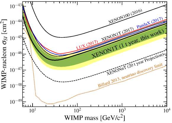
Figure 13: Current results of direct searches for WIMPs: best limits on spin-independent WIMP-nucleus cross section per nucleon come from XENON-1T experiment [34]. Note that cross section $10^{-10}~{}\mbox{nbarn}=10^{-43}~{}\mbox{cm}^{2}$ in the lower part of Fig. 12 is in the upper part of this figure.

Figure 14 shows both current limits (solid lines) and projected sensitivities of future dark matter detection experiments, again for spin-independent interactions [10]. We see that, on the one hand, the progress in experimental search is truly remarkable, and, on the other, the null results of this search are becoming alarming. The null results of direct (and also indirect, see below) searches are particularly worrying in view of null results of SUSY searches at the LHC.

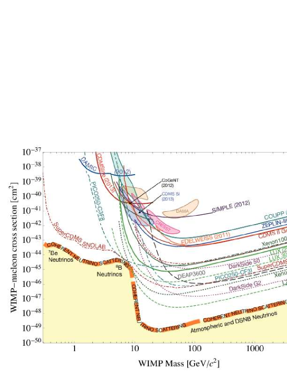
Figure 14: Current limits and projected sensitivities of direct searches for WIMPs (spin-independent WIMP-nucleus cross section per nucleon). Yellow band in the lower part is “neutrino floor”, at which interactions of cosmic neutrinos become an important background.

6.3 Ad hoc WIMP candidates; indirect searches and the LHC

In view of the strong direct detection limits and null results of the SUSY searches at the LHC, it makes sense to consider less motivated, ad hoc WIMP candidates. The simplest assumption is that WIMP is not nearly degenerate with any other new particle, so that the calculation of its abundance outlined above applies, and that there is one particle that mediates its pair-annihilation. This mediator can be either a Standard Model particle or a new one; we give examples of both cases. The models of this sort are often called simplified. We emphasize that the two examples of simplified models which we are going to discuss do not exhaust all possible WIMPs and mediators. Some of the models that we leave aside are actually consistent with both cosmology (they give the right value of $\Omega_{DM}$) and experimental limits. The study of numerous simplified models is given, e.g., in Ref. [11].

With this reservation, it is fair to say that many simplified models are either already ruled out or will be ruled out soon. As one illustration, we consider “Higgs portal”, a set of models where the only field which interacts directly with WIMPs is Englert–Brout–Higgs field. The lowest dimension Higgs-WIMP interaction terms in the cases of spin-0 WIMP $\chi$ and spin-1/2 WIMP $\psi$ are

$$\lambda^{H}_{\chi}\chi^{*}\chi H^{\dagger}H\;,\;\;\;\;\;\;\frac{\lambda^{H}_{\psi}}{\Lambda}\bar{\psi}\psi H^{\dagger}H\;,$$

where $H$ is EBH field. Here $\lambda^{H}_{\chi}$, $\lambda^{H}_{\psi}$ are dimensionless parameters, while $\Lambda$ has dimension of mass. In both cases $\chi$ ($\psi$) is a Standard Model singlet with zero weak hypercharge; it has “hard” mass $m_{\chi(\psi)}$. Since the vacuum expectation value of EBH field $H$ is non-zero, the above interaction terms induce trilinear WIMP-WIMP-Higgs responsible for $s$-channel WIMP annihilation via the Higgs exchange. It is this annihilation that is relevant in the early Universe. The trouble is that almost entire parameter space of the Higgs portal is ruled out by direct searches. This is illustrated in Fig. 15, Ref. [11].

           

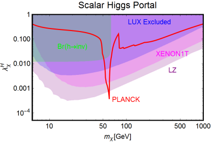
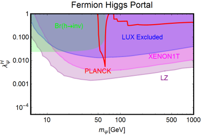
Figure 15: Predictions from dark matter abundance (red solid lines labeled “PLANCK”) and direct detection limits (shadows) in the Higgs portal models [11]. Left panel: spin-0 WIMP; right panel: spin-1/2 WIMP.

Another illustration is $Z^{\prime}$-portal. One assumes that both WIMP (say, spin-1/2 particle $\psi$) and Standard Model fermions interact with a new vector boson $Z^{\prime}$:

$$g_{\psi}\bar{\psi}(V_{\psi}-A_{\psi}\gamma^{5})\psi Z^{\prime}+\sum_{f}\,g_{f}\bar{f}(V_{f}-A_{f}\gamma^{5})f\,Z^{\prime}\;,$$ (42)

where sum runs over all Standard Model fermions (important role is played by quarks). The coupling constants $g_{\psi}$, $g_{f}$ are often chosen to be of order 0.5, as suggested by GUTs. Almost all parameter space of $Z^{\prime}$-portal models with $V_{\psi}\neq 0$ is also ruled out by direct searches [11], as shown in Fig. 16.

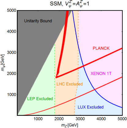
Figure 16: Same as in Fig. 15 but for $Z^{\prime}$-portal (42) with $g_{\psi}=g_{f}=0.65$ and $V_{\psi}=A_{\psi}=V_{f}=A_{f}=1$.

The situation is better in models with axial-vector interactions of new vector boson (we still call it $Z^{\prime}$) with both the Standard Model particles and WIMPs,

$$V_{\psi}=V_{f}=0\;.$$

In that case, interaction of WIMPs with nucleons is spin-dependent, the elastic WIMP-nucleus cross section is not enhanced by $A^{2}$, so the direct detection limits are not as strong as in the case of spin-independent interaction. An important player here is the LHC, whose limits are the most stringent [11], see Fig. 17. We see from Fig. 17 that models with $M_{Z^{\prime}}\gtrsim 2.8$ TeV are capable of producing the correct abundance of dark matter and at the same time are not ruled out experimentally.

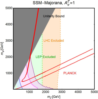
Figure 17: Same as in Fig. 16 but for axial-vector $Z^{\prime}$-portal (42) with and $V_{\psi}=V_{f}=0$, $A_{\psi}=A_{f}=1$.

Another way of comparing current sensitivities of direct and LHC searches is given in Figs. 18, 19. The plots (compiled by ATLAS collaboraion) refer to the model (42) with vector boson $Z^{\prime}$ and coupling constants with quarks $g_{q}$, leptons $g_{l}$ and WIMPs $g_{\psi}\equiv g_{\chi}$ whose values are written in figures. Figure 18 shows the limits in the vector case, $A_{\psi}=A_{f}=0$, $V_{\psi}=V_{f}=1$, while Fig. 19 refers to axial-vector case $A_{\psi}=A_{f}=1$, $V_{\psi}=V_{f}=0$. Clearly, the direct searches are more sensitive than the LHC in vector case (spin-independent WIMP-nucleon elastic cross section), while the LHC wins in the axial-vector case (spin-dependent elastic cross section). Overall, the LHC has become an important source of limits on WIMPs.

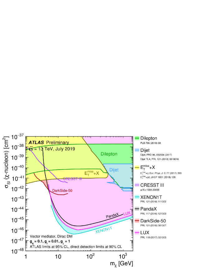
Figure 18: LHC and direct detection limits in the case of spin-independent WIMP-nucleon elastic cross section.

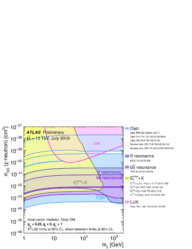
Figure 19: The same as in Fig. 18 but for spin-dependent WIMP-nucleon elastic cross section.

Besides direct and LHC searches for cosmic and collider-produced WIMPs, respectively, important ways to address WIMPs are indirect searches. One approach is to search for high energy $\gamma$-rays which are produced in annihilations of WIMPs in various cosmic sources, from dwarf galaxies to Galactic center to clusters of galaxies, and also diffuse $\gamma$-ray flux coming from the entire Universe. This approach is particularly relevant if WIMP annihilation proceeds in $s$-wave: in that case the non-relativistic annihilation rate is determined by (41), which is velocity-independent (modulo possible Sommerfeld enhancement, see Ref. [35] for detailed discussion). On the contrary, for $p$-wave annihilation the rate $\sigma v$ is proportional to $v^{2}$, and since the velocities in the sources are small ($v^{2}\lesssim 10^{-6}$ as compared to $v^{2}\simeq 0.1$ relevant to (41)), the annihilation cross section is strongly suppressed in the present Universe. Thus, meaningful limits are obtained by $\gamma$-ray observatories for WIMPs annihilating in $s$-wave. The current situation and future prospects are illustrated in Fig. 20, Ref. [10]. The assumption that enters this compilation is that the major WIMP annihilation channel is $b\bar{b}$. Clearly, already existing instruments, and to even larger extent future experiments are sensitive to a wide class of WIMP models.

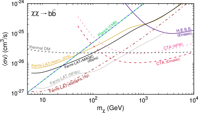
Figure 20: Limits on WIMP annihilation cross section obtained by $\gamma$-ray telescopes (solid lines) and projected sensitivities of future $\gamma$-ray observatories (dashed lines). “NFW” and “Einasto” refer to different dark matter profiles in galaxies. Dashed line “thermal DM” is the predicion from cosmology (41) under assumption of $s$-wave annihilation. Note the different units for $\langle\sigma v\rangle$ used in this figure and in (41).

Indirect searches for dark matter WIMPs include the search for neutrinos coming from the centers of the Earth and Sun (WIMPs may concentrate and annihilate there), see, e.g., Ref. [36], positrons and antiprotons in cosmic rays (produced in WIMP annihilations in our Galaxy), see, e.g., Ref. [37]. These searches have produced interesting, albeit model-dependent limits on WIMP properties.

6.4 WIMP summary

• While WIMP hypothesis was very attractive for long time, and SUSY neutralino was considered the best candidate, today the WIMP option is highly squeezed. On the one hand, the parameter space of most of the concrete models is strongly constrained by direct, LHC and indirect searches. On the other hand, SUSY searches at the LHC have moved colored superpartner masses into TeV region, thus making SUSY less attractive from the viewpoint of solving the gauge chierarchy problem.

• This does not mean too much, however: we would like to discover one theory and one point in its parameter space.

• Hunt for WIMPs continues in numerous directions. Their potential is far from being exhausted. Concerning direct searches, we will soon face the neutrino floor problem – the situation where cosmic neutrino background will show up. It is time to look into ways to go beneath the neutrino floor.

• With null results of WIMP searches, it makes a lot of sense to strengthen also searches for other dark matter candidates.

7 Axions

Axion is a consequence of the Peccei–Quinn solution to the strong CP-problem. It is a pseudo-Nambu–Goldstone boson of an approximate Peccei–Quinn symmetry.

7.1 Strong CP problem

To understand the strong CP-problem, we begin with considering QCD in the chiral limit $m_{u}=m_{d}=m_{s}=0$. The Lagrangian is

$$L_{QCD,m=0} =-\frac{1}{4}G_{\mu\nu}^{a}G^{a\mu\nu}+\sum_{i}\bar{q}_{i}i\gamma^{\mu}D_{\mu}q_{i}$$

$$=-\frac{1}{4}G_{\mu\nu}^{a}G^{a\mu\nu}+\sum_{i}\left(\bar{q}_{L,i}i\gamma^{\mu}D_{\mu}q_{L,i}+\bar{q}_{R,i}i\gamma^{\mu}D_{\mu}q_{R,i}\right)\;,$$

where $i=u,d,s$. As it stands, it is invariant under independent transformations of left and right quark fields $q_{L,i}$ and $q_{R,i}$, each with arbitrary unitary matrices. Naively, this means that the theory possesses large symmetry

$$SU(3)_{L}\times U(1)_{L}\times SU(3)_{R}\times U(1)_{R}=SU(3)_{L}\times SU(3)_{R}\times U(1)_{B}\times U(1)_{A}$$ (43)

where vector $U(1)_{B}$ is baryon number symmetry, $q_{i}\to{\rm e}^{i\alpha}q_{i}$, while axial $U(1)_{A}$ act as $q_{i}\to{\rm e}^{i\beta\gamma^{5}}q_{i}$.

The symmtery (43) is spontaneously broken: there exist quark condensates in QCD vacuum:

$$\langle\bar{u}_{L}u_{R}\rangle=\langle\bar{d}_{L}d_{R}\rangle=\langle\bar{s}_{L}s_{R}\rangle=\frac{1}{2}\langle\bar{q}q\rangle\sim\Lambda_{QCD}^{3}$$ (44)

The unbroken symmetry $SU(3)_{V}$ rotates left and right quarks together (this is the well known flavor $SU(3)$); $U(1)_{B}$ also remains unbroken.

Spontaneous breaking of global symmetry always leads to the presence of Nambu–Goldstone bosons. Naively, one expects that there are 9 Nambu–Goldstone bosons: 8 of them come from symmetry breaking $SU(3)_{L}\times SU(3)_{R}\to SU(3)_{V}$, and one from $U(1)_{B}\times U(1)_{A}\to U(1)_{B}$ (since the original symmetry is explicitly broken by quark masses, these should be pseudo-Nambu–Goldstone bosons with non-zero mass). However, there are only 8 light pseudoscalar particles whose properties are well described by Nambu–Goldstone theory: these are $\pi^{\pm}$, $\pi^{0}$, $K^{\pm}$, $K^{0}$, $\bar{K}^{0}$, $\eta$. Indeed, their masses squared are proportional to quark masses, e.g., $m_{\pi}^{2}=(m_{u}+m_{d})\langle\bar{q}q\rangle/f_{\pi}^{2}$. Importantly, yet another pseudoscalar $\eta^{\prime}$ is heavy and does not behave like pseudo-Nambu–Goldstone boson.

The reason for this mismatch (absence of the 9th pseudo-Nambu–Goldstone boson) is that $U(1)_{A}$ is not, in fact, a symmetry of QCD even in the chiral limit. The corresponding axial current suffers, at the quantum level, Adler–Bell–Jackiw (triangle, or axial) anomaly,

$$\partial_{\mu}J_{A}^{\mu}\neq 0\;.$$

This means that the axial charge is not conserved, and thus the $U(1)_{A}$ is explicitly broken. We discuss this phenomenon in little more detail in Sec. 10.2 in the conext of electroweak baryon number non-conservation.

The strong CP-problem [38, 39, 40] emerges in the following way. One considers quark mass terms in the Standard Model Lagrangian, which are obtained from the Yukawa interaction terms with non-zero Higgs expectation value. The common lore is that one can perform unitary rotations of quark fields to make quark mass terms real (and in this way generate CKM matrix in quark interactions with $W$-bosons). This is not quite true, precisely because one cannot freely use $U(1)_{A}$-rotation. In fact, by performing $SU(3)_{L}\times SU(3)_{R}\times U(1)_{B}$-rotation, one casts the mass term of light quarks into the form

$$L_{m}=\mbox{e}^{i\theta}\cdot m_{ij}^{CKM}\bar{q}_{L,i}q_{R,j}+h.c.\;,$$

where $m_{ij}^{CKM}=\mbox{diag}(m_{u},m_{d},m_{s})$ is real diagonal matrix, and $\theta$ is some phase. Naively, this phase can be rotated away by axial rotation of all three light quark fields, $q_{i}\to\mbox{e}^{-i\theta\gamma_{5}/2}q_{i}$, but, as we discussed, this is not an innocent field redefinition. What happens instead is that this transformation generates an extra term in the QCD Lagrangian

$$\Delta L=\frac{\alpha_{s}}{8\pi}\cdot\theta\cdot G_{\mu\nu}^{a}\tilde{G}^{\mu\nu\;a}\;,$$ (45)

where $\alpha_{s}$ is the $SU(3)_{c}$ gauge coupling, $G_{\mu\nu}^{a}$ is the gluon field strength, $\tilde{G}^{\mu\nu\;a}=\frac{1}{2}\epsilon^{\mu\nu\lambda\rho}G^{a}_{\lambda\rho}$ is the dual tensor. The term (45) is invariant under gauge symmetries of the Standard Model, but it violates P and CP. Similar term, but with another parameter $\theta_{0}$ instead of $\theta$, can already exist in the initial QCD Lagrangian. The combined parameter

$$\bar{\theta}=\theta+\theta_{0}$$

is a “coupling constant” that cannot be removed by field redefinition, and QCD with non-zero $\bar{\theta}$ violates CP.

Let us show explicitly that the parameter $\bar{\theta}$ is physical, i.e., some physical quantities depend on $\bar{\theta}$. To this end, we perform chiral rotation of light quark fields $q_{i}\to\mbox{e}^{+i\bar{\theta}\gamma_{5}/2}q_{i}$ to get rid of the term (45) and generate the phase in the quark mass terms

$$L_{m}=\sum_{i}\mbox{e}^{i\bar{\theta}}m_{i}\bar{q}_{L,i}q_{R,i}+h.c.$$

Let us consider for simplicity two light quark flavors $u$ and $d$ with equal masses $m_{u}=m_{d}\equiv m_{q}\sim 4$ MeV and calculate the vacuum energy density in such a theory. We use perturbation theory in quark masses, and work to the leading order. Then the $\bar{\theta}$-dependent part of the vacuum energy density is $V(\bar{\theta})=-\langle L_{m}\rangle$. We recall that $\langle\bar{q}q\rangle$ is non-zero in the chiral limit, see (44), and observe that it is real, provided that the term (45) is absent (no spontaneous CP-violation in the chiral limit). Importantly, $\langle\bar{q}q\rangle$ does not have an arbitrary phase, since the arbitrariness of this phase would mean that $U(1)_{A}$ is a (spontaneously broken) symmetry, which is not the case, as we discussed above. Thus, we obtain

$$V(\bar{\theta})=-\langle L_{m}\rangle=-2m_{q}\langle\bar{q}q\rangle\cos\bar{\theta}=-\frac{m_{\pi}^{2}f_{\pi}^{2}}{4}\cos\bar{\theta}\;.$$ (46)

This shows explicitly that $\bar{\theta}$ is a physically relevant parameter. We note in passing that the expression for $V(\bar{\theta})$ is, in fact, more complicated, especially for $m_{u}\neq m_{d}$ and also for three quark flavors, but the main property — minimum at $\bar{\theta}=0$ — is intact.

Thus, $\bar{\theta}$ is a new coupling constant that can take any value in the interval $(-\pi,\pi)$. There is no reason to think that $\bar{\theta}=0$. The term (45) has a dramatic phenomenological consequence: it generates electric dipole moment (EDM) of neutron $d_{n}$, which is estimated as [41]

$$d_{n}\sim\bar{\theta}\cdot 10^{-16}\cdot e\cdot\mbox{cm}\;.$$ (47)

Neutron EDM is strongly constrained experimentally,

$$d_{n}\lesssim 3\cdot 10^{-26}\cdot e\cdot\mbox{cm}\;.$$ (48)

This leads to the bound on the parameter $\bar{\theta}$,

$$|\bar{\theta}|<0.3\cdot 10^{-9}\;.$$

The problem to explain so small value of $\bar{\theta}$ is precisely the strong CP-problem.

A solution to this problem does not exist within the Standard Model. The solution is offered by models with axion. The idea of these models is to promote $\bar{\theta}$-parameter to a field, which is precisely the axion field. This can be done in various ways. Two well-known ones are Dine–Fischler–Srednicki–Zhitnitsky [45, 46] (DFSZ) and Kim–Shifman–Vainshtein–Zakharov [47, 48] (KSVZ) mechanisms. In either case, one introduces a complex scalar field $\Phi$ and makes sure that without QCD effects, the theory is invariant under global Peccei–Quinn $U(1)_{PQ}$ symmetry. Under this symmetry, the field $\Phi$ transforms as $\Phi\to\mbox{e}^{i\alpha}\Phi$. One also arranges that the QCD effects make this symmetry anomalous, very much like $U(1)_{A}$, so that under the $U(1)_{PQ}$-transformation, the Lagrangian obtains an additional contribution

$$\Delta L=C\frac{\alpha_{s}}{8\pi}\cdot\alpha\cdot G_{\mu\nu}^{a}\tilde{G}^{\mu\nu\;a}\;,$$ (49)

where $C$ is a model-dependent constant of order 1. A simple example is KSVZ model: one adds a new quark $\psi$ which interacts with $\Phi$ as follows:

$$L_{int}=h\Phi\bar{\psi}_{L}\psi_{R}+h.c.$$ (50)

where $h$ is Yukawa coupling. Then the Peccei–Quinn transformation is

$$\Phi\to\mbox{e}^{i\alpha}\Phi\;,\;\;\;\;\;\psi\to\mbox{e}^{i\alpha\gamma^{5}/2}\psi\;,$$

while “our” quark fields are $U(1)_{PQ}$-singlets. In the same way as above, this transformation induces the term (49), as required.

Now, one arranges the scalar potential for $\Phi$ in such a way that the Peccei–Quinn symmetry is spontaneously broken at very high energy. If not for QCD effects, the phase of $\Phi$ would be a massless Nambu–Goldstone boson, the axion. At low energies one writes $\Phi=f_{PQ}\cdot\mbox{e}^{i\theta(x)}$, where $f_{PQ}$ is the Peccei–Quinn vacuum expectation value. In the absence of QCD, the field $\theta$ is rotated away from the non-derivative part of the action by the Peccei–Quinn rotation, while it reappears in the form (49) when QCD is switched on. We see that the parameter $\bar{\theta}$ is indeed promoted to a field, and this parameter disappeas upon shifting $\theta(x)\to\theta(x)-\bar{\theta}$; we are free to set $\bar{\theta}=0$. Now, there is a potential for the field $\theta$; it is given precisely by eq. (46) with $\bar{\theta}$ replaced by $\theta$. Hence, the low energy axion Lagrangian reads

$$L_{a}=\frac{f^{2}_{PQ}}{2}\partial_{\mu}\theta\partial^{\mu}\theta-V(\theta)\;.$$

As usual, the first term here comes from the kinetic term for the field $\Phi$. We recall that the minimum of $V(\theta)$ is at $\theta=0$; at this value CP is not violated, the strong CP problem is solved! We now make field redefinition, $\theta=a/f_{PQ}$ and find from (46) that the quadratic axion Lagrangian is

$$L_{a}=\frac{1}{2}\partial_{\mu}a\partial^{\mu}a-\frac{m_{a}^{2}}{2}a^{2}\;,$$

where

$$m_{a}=\frac{m_{\pi}f_{\pi}}{2f_{PQ}}\;.$$ (51)

The axion is pseudo-Nambu-Goldstone boson.

To summarize, for large Peccei–Quinn scale $f_{PQ}\gg M_{W}$, axion is a light particle whose interactions with the Standard Model fields are very weak. Like for any Nambu–Goldstone field, the tree-level interactions of axion with quarks and leptons are described by the generalized Goldberger–Treiman formula

$$L_{af}=\frac{1}{f_{PQ}}\cdot\partial_{\mu}a\cdot J^{\mu}_{PQ}\;.$$ (52)

Here

$$J^{\mu}_{PQ}=\sum_{f}e^{(PQ)}_{f}\cdot\bar{f}\gamma^{\mu}\gamma^{5}f\;.$$ (53)

The contributions of fermions to the current $J^{\mu}_{PQ}$ are proportional to their PQ charges $e^{(PQ)}_{f}$; these charges are model-dependent. There is necessarily interaction of axions with gluons, see (49),

$$L_{ag}=C_{g}\frac{\alpha_{s}}{8\pi}\cdot\frac{a}{f_{PQ}}\cdot G_{\mu\nu}^{a}\tilde{G}^{\mu\nu\;a}$$ (54)

Finally, there is axion-photon coupling

$$L_{a\gamma}=g_{a\gamma\gamma}\cdot aF_{\mu\nu}\tilde{F}^{\mu\nu}\;,\;\;\;\;\;g_{a\gamma\gamma}=C_{\gamma}\frac{\alpha}{8\pi f_{PQ}}\;,$$ (55)

The dimensionless constants $C_{g}$ and $C_{\gamma}$ are model-dependent and, generally speaking, not very much different from 1. The main free parameter is $f_{PQ}$, while the axion mass is related to it via eq. (51); numerically,

$$m_{a}=6~{}\mu\mbox{eV}~{}\cdot\left(\frac{10^{12}~{}\mbox{GeV}}{f_{PQ}}\right)\;.$$ (56)

There are astrophysical bounds on the strength of axion interactions $f_{PQ}^{-1}$ and hence on the axion mass. Axions in theories with $f_{PQ}\lesssim 10^{9}$ GeV, which are heavier than about $10^{-2}$ eV, would be intensely produced in stars and supernovae explosions. This would lead to contradictions with observations. So, we are left with very light axions, $m_{a}\lesssim 10^{-2}$ eV. These very light and very weakly interacting axions are interesting dark matter candidates.

7.2 Axions in cosmology

Axions can serve as dark matter if they do not decay in the lifetime of the Universe. The main decay channel of the light axion is decay into two photons. The axion width is calculated as

$$\Gamma_{a\to\gamma\gamma}=\frac{m_{a}^{3}}{4\pi}\left(C_{\gamma}\frac{\theta}{8\pi f_{PQ}}\right)^{2}\;,$$

where the quantity in parenthesis is the axion-photon coupling, see (55). We recall the relation (51) and obtain axion lifetime

$$\tau_{a}=\frac{1}{\Gamma_{a\to\gamma\gamma}}=\frac{64\pi^{3}m_{\pi}^{2}f_{\pi}^{2}}{C_{\gamma}^{2}\alpha^{2}m_{a}^{5}}\sim 10^{24}~{}\mbox{s}~{}\cdot\left(\frac{\mbox{eV}}{m_{a}}\right)^{5}\;.$$

By requiring that this lifetime exceeds the age of the Universe, $\tau_{a}>t_{0}\approx 14$ billion years, we find a very weak bound on the mass of axion as dark matter candidate, $m_{a}<25~{}\mbox{eV}$.

Thermal production of axions in the early Universe not very relevant, since even if they were in thermal equilibrium at high temperatures, their thermally produced present number density is substantially smaller than that of photons and neutrinos, and with their tiny mass they do not contribute much into the energy density. This is a welcome property, since thermally produced axions, if they composed substantial part of dark matter, would be hot dark matter, which is ruled out.

There are at least two mechanisms of axion production in the early Universe that can provide not only right axion abundance but also small initial velocities of axions. The latter property makes axion a cold dark matter candidate, despite its very small mass.

One mechanism [50, 51, 52] is called misalignment scenario. It assumes that the Peccei–Quinn symmetry is spontaneously broken before the beginning of the hot epoch, $\langle\Phi\rangle\neq 0$. This is indeed the case in inflationary framework, if $f_{PQ}$ is higher than both inflationary Hubble parameter (towards the inflation end) and the reheat temperature of the Universe. In this case the axion field (the phase of the field $\Phi$) is homogeneous over the entire visible universe, and initially it can take any value $\theta_{0}$ between $-\pi$ and $\pi$. As we have seen in (46), the axion potential is proportional to the quark condensate $\langle\bar{q}q\rangle$. This condensate vanishes at high temperatures, $T\gg\Lambda_{QCD}$, and the axion potential is negligibly small. As the temperature decreases, the axion potential builds up. Accordingly, the axion mass increases from zero to $m_{a}$; hereafter $m_{a}$ denotes the zero-temperature axion mass. The axion field practically does not evolve when $m_{a}(T)\ll H(T)$ and at the time when $m_{a}(T)\sim H(T)$ it starts to roll down from the initial value $\theta_{0}$ to the minimum $\theta=0$ and then it oscillates. During all these stages of evolution, the axion field is homogeneous in space. The homogeneous oscillating field can be interpreted as a collection of scalar quanta with zero spatial momenta, the axion condensate. This is indeed cold dark matter.

Let us estimate the present energy density of axion field in this picture. The oscillations start at the time $t_{osc}$ when $m_{a}(t_{osc})\sim H(t_{osc})$. At this time, the energy density of the axion field is estimated as

$$\rho_{a}(t_{osc})\sim m_{a}^{2}(t_{osc})a_{0}^{2}=m_{a}^{2}(t_{osc})f_{PQ}^{2}\theta_{0}^{2}\;.$$

The number density of axions at rest at the beginning of oscillations is estimated as

$$n_{a}(t_{osc})\sim\frac{\rho_{a}(t_{osc})}{m_{a}(t_{osc})}\sim m_{a}(t_{osc})f_{PQ}^{2}\theta_{0}^{2}\sim H(t_{osc})f_{PQ}^{2}\theta_{0}^{2}\;.$$

This number density, as any number density of non-relativistic particles, then decreases as $a^{-3}$. Axion-to-entropy ratio at time $t_{osc}$ is

$$\frac{n_{a}}{s}\sim\frac{H(t_{osc})f_{PQ}^{2}}{\frac{2\pi^{2}}{45}g_{*}T_{osc}^{3}}\cdot\theta_{0}^{2}\simeq\frac{f_{PQ}^{2}}{\sqrt{g_{*}}T_{osc}M_{Pl}}\cdot\theta_{0}^{2}\;,$$

where we use the usual relation $H=1.66\sqrt{g_{*}}T^{2}/M_{Pl}$. The axion-to-entropy ratio remains constant after the beginning of oscillations, so the present mass density of axions is

$$\rho_{a,0}=\frac{n_{a}}{s}m_{a}s_{0}\simeq\frac{m_{a}f_{PQ}^{2}}{\sqrt{g_{*}}T_{osc}M_{Pl}}s_{0}\cdot\theta_{0}^{2}\;.$$ (57)

To obtain a simple estimate, let us set $T_{osc}\sim\Lambda_{QCD}\simeq 200~{}\mbox{MeV}$ and make use of (56). We find

$$\Omega_{a}\equiv\frac{\rho_{a,0}}{\rho_{c}}\simeq\left(\frac{10^{-6}~{}\mbox{eV}}{m_{a}}\right)\theta_{0}^{2}\;.$$ (58)

The natural assumption about the initial phase is $\theta_{0}\sim\pi/2$. Hence, axion of mass $m_{a}=(\mbox{a~{}few})\cdot 10^{-6}$ eV is a good dark matter candidate. Note that axion of lower mass $m_{a}<10^{-6}$ eV may also serve as dark matter particle, if for some reason the initial phase $\theta_{0}$ is much smaller than $\pi/2$.

More precise estimate is obtained by taking into account the fact that that the axion mass smoothly depends on temperature:

$$\Omega_{a}\simeq 0.2\cdot\theta_{0}^{2}\cdot\left(\frac{4\cdot 10^{-6}~{}\mbox{eV}}{m_{a}}\right)^{1.2}$$

We see that our crude estimate (58) is fairly accurate.

We note that in the misalignment scenario, and in the inflationary framework, the initial phase $\theta_{0}$ is not quite homogeneous in space. At inflationary stage, vacuum fluctuations of all massless or light scalar fields get enhanced. As a result, scalar fields become inhomogeneous on scales exceeding the inflationary Hubble scale $H_{infl}^{-1}$. The amplitudes of these inhomogeneities (for canonically normalized fields) are equal to $H_{infl}/(2\pi)$. Phase perturbations give rise to perturbations of axion dark matter energy density, which are uncorrelated with perturbations of conventional matter. These uncorrelated dark matter perturbations are called isocurvature (or entropy) modes. Cosmological observations show that their contribution cannot exceed a few per cent of the dominant adiabatic mode. This leads to a constraint [53] on inflationary Hubble parameter $H_{infl}$ or, equivalently, on the energy scale of inflation (energy density of the inflaton field)

$$V_{infl}^{1/4}\lesssim 10^{13}~{}\mbox{GeV}\;.$$

This makes the misalignment mechanism somewhat contrived. Reversing the argument, detection of the dark matter entropy mode would be an interesting hint towards the nature of dark matter.

Another mechanism of axion production in the early Universe works under the assumption which is opposite to the main assumption of the misalignment scenario. Namely, one assumes that the Peccei–Quinn symmetry is restored at the beginning of hot epoch, and gets spontaneously broken at temperature of order $T\sim f_{PQ}$ at hot stage. Then the phase of the field $\Phi$ is uncorrelated at distances exceeding the size of the horizon at that time. In principle, one should be able to predict the value of $f_{PQ}$ and hence $m_{a}$ in this scenario, since there is no uncertainty in the initial conditions. However, the dynamics in this case is quite complicated. Indeed, the uncorrelated phase gives rise to the production of global cosmic strings [54] — topological defects that exist in theories with spontaneously broken global $U(1)$ symmetry ($U(1)_{PQ}$ in our case; for a discussion see, e.g., Ref. [55]). At the QCD transition epoch, defects of another type, axion domain walls, are created. Then all these defects get destructed, giving rise to the production of axions. The analysis of this dynamics has been made by various authors, see, e.g., Refs. [56, 57], but it is fair to say that there is no compelling prediction for $m_{a}$ yet. A reasonable estimate of the axion mass is (Ref. [56] claims $m_{a}=2.6\cdot 10^{-5}$ eV)

$$m_{a}=(\mbox{a~{}few})\cdot 10^{-5}~{}\mbox{eV}\;.$$

To end up with cosmological aspects of axion dark matter, we note that it has interesting phenomenology in the present Universe. Axions tend to form mini-clusters [58] which can be disrupted and form streams of dark matter [59]. Axions also form bose-stars [60]. All this exotica is relevant to both astrophysics and axion search.

7.3 Axion search

Search for dark matter axions with mass $m_{a}\sim 10^{-5}-10^{-6}$ eV is difficult, but not impossible. One way is to search for axion-photon conversion in a resonant cavity filled with strong magnetic field. Indeed, in the background magnetic field, the axion-photon interaction (55) leads to the conversion $a\to\gamma$, see Fig. 21.

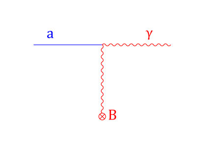
Figure 21: Axion-photon conversion in magnetic field.

Axions of mass $10^{-5}-10^{-6}$ eV are converted to photons of frequency $\nu=m/(2\pi)=2-0.2$ GHz (radiowaves; $m=10^{-6}~{}\mbox{eV}\longleftrightarrow\nu=240$ MHz). To collect reasonable number of conversion photons, one needs cavities of high quality factor $Q$, which have small bandwidths. This means that one goes in small steps in $m_{a}$, and the whole search takes long time. This is illustrated in Fig. 22.

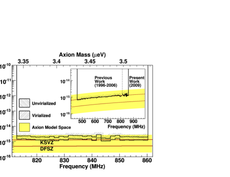
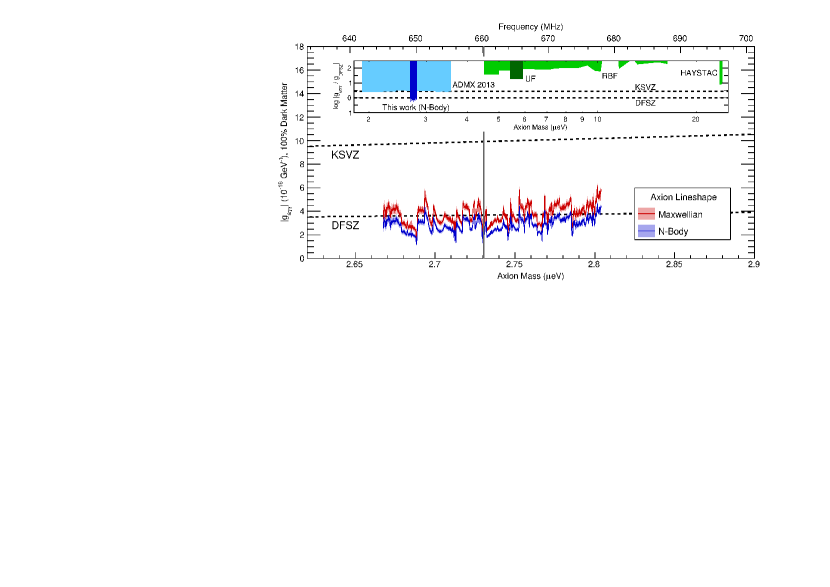
Figure 22: Limits on the axion-photon coupling for various axion masses. Lines labeled KSVZ and DSVZ refer to predictions of the two axion models under the assumption that axions make the whole of dark matter. Shown are limits published by ADMX collaboration in 2010 [61] (upper panel) and in 2018 [62]. Note the limited ranges of masses spanned durin the long period of time. Note also that the recent limits (lower panel) reach almost entire range of axion-photon couplings predicted by varios axion models.

The hunt for dark matter axions has been intensified recently. A new set of resonant cavity experiments, CAPP, is under preparation, see Fig. 23. A new approach to search for heavier dark matter axions with $m_{a}\gtrsim 4\cdot 10^{-5}$ eV has been suggested by MADMAX interest group [64]. Other axion search experiments are reviewed in Refs. [63, 65].

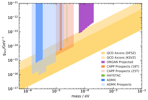
Figure 23: Future prospects of dark matter axion search with resonant cavities [63].

7.4 Axion-like particles (ALPs)

There may exist light, weakly interacting scalar or pseudoscalar particles other than axions. They are called axion-like particles, ALPs, and they may emerge as pseudo-Nambu–Goldstone bosons of some new approximate global symmetry. We have discussed one example, fuzzy dark matter, in Sec. 5.2. Unlike the axion case, where axion-photon coupling is related, albeit in somewhat model-dependent way, to its mass via eqs. (55) and (56), ALP mass and coupling to photons are both arbitrary parameters. Also, ALPs may interact with the Standard Model fermions, and that coupling is again a free parameter. ALPs may or may not be dark matter candidates; search for them is of interest independently of dark matter problem.

If ALP is a dark matter candidate, instruments described in previous subsection — “haloscopes” — are capable for searching for dark matter ALPs, and it makes sense to extend the search to as wide mass range as possible. In this regard, it is worth mentioning that CASPEr experiment [66] is going to be sensitive to very light ALPs, $m\lesssim 10^{-9}$ eV, and very small ALP-fermion couplings.

ALPs may be produced in the Sun, and their flux may be detectable by “helioscopes”, instruments searching for the axion-photon conversion in the magnetic field of a magnet looking at the Sun. One such instrument, CAST, has been operating for long time, whereas other experiments, IAXO and TASTE, are planned. Another way to search for ALPs makes use of the idea of “light shining through a wall”, see Fig. 24; this idea is implemented in ALPS-I, ALPS-II expertiments. For a review of these approaches see, e.g., Ref. [65]. Finally, ALPs can be searched in beam-dump experiments and in decays of $K$- and $B$-mesons. Interesting limits are obtained by CHARM and BaBar experiments, and a promising planned experiment is SHiP at CERN [67].

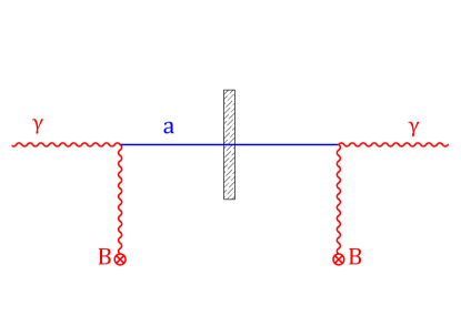
Figure 24: “Light shining through a wall”: laser light shining from the left is converted into axions in magnetic field of a magnet placed before the wall, axions pass through the wall and are converted into photons by a magnet behind the wall; the latter photons are detected by highly sensitive photon detector.

Bounds and propects for search for light ALPs are summarized Fig. 25.

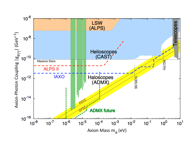
Figure 25: Bounds on ALPs: ALP-photon coupling vs ALP mass [65]. Inclined straight strip with lines labeled “KSVZ” and “DFSZ” is the range of predictions of axion models. Shaded regions are limits from existing experiments, dashed lines show sensitivities of future searches.

8 Warm dark matter: sterile neutrinos

As we discussed in Section 5.1, there are arguments, albeit not yet conclusive, which favor warm, rather than cold, dark matter. If WDM particles were in kinetic equilbrium at some epoch in the early Universe, then their mass should be in the range $3-10$ keV. Reasonably well motivated particles of this mass are sterile neutrinos.

Sterile neutrinos — massive leptons $N$ which do not participate in the Standard Model gauge interactions — are most probably required for giving masses to ordinary, “active” neutrinos. The masses of sterile neutrinos cannot be predicted theoretically. Although sterile neutrinos of WDM mass $m_{N}=3-10$ keV are not particularly plausible from particle physics prospective, they are not pathological either. In the simplest case the creation of sterile neutrino states $|N\rangle$ in the early Universe occurs due to their mixing with active neutrinos $|\nu_{\alpha}\rangle$, $\alpha=e,\mu,\tau$. In the approximation of mixing between two states only, we have

$$|\nu_{\alpha}\rangle=\cos\theta|\nu_{1}\rangle+\sin\theta|\nu_{2}\rangle\;,\;\;\;\;\;|N\rangle=-\sin\theta|\nu_{1}\rangle+\cos\theta|\nu_{2}\rangle\;,$$

where $|\nu_{\alpha}\rangle$ and $|N\rangle$ are active and sterile neutrino states, $|\nu_{1}\rangle$ and $|\nu_{2}\rangle$ are mass eigenstates of masses $m_{1}$ and $m_{2}$, where we order $m_{1}<m_{2}$, and $\theta$ is the vacuum mixing angle between sterile and active neutrino. This mixing should be weak, $\theta\ll 1$, otherwise sterile neutrinos would decay too rapidly, see below. The heavy state is mostly sterile neutrino $|\nu_{2}\rangle\approx|N\rangle$, and $m_{2}\equiv m_{N}$ is the sterile neutrino mass.

The calculation of sterile neutrino abundance is fairly complicated, and we do not reproduce it here. If there is no sizeable lepton asymmetry in the Universe, the estimate is

$$\Omega_{N}\simeq 0.2\cdot\left(\frac{\sin\theta}{10^{-4}}\right)^{2}\cdot\left(\frac{m_{N}}{1~{}\mbox{keV}}\right)^{2}\;.$$ (59)

The energy spectrum of sterile neutrinos is nearly thermal. Thus, sterile neutrino of mass $m_{\nu}\gtrsim 1$ keV and small mixing angle $\theta_{\alpha}\lesssim 10^{-4}$ would serve as dark matter candidate. However, this range of masses and mixing angles is ruled out. The point is that due to its mixing with active neutrino, sterile neutrino can decay into active neutrino and photon, see Fig. 26.

$$N\to\nu_{\alpha}+\gamma\;.$$

The sterile neutrino decay width is proportional to $\sin^{2}\theta$.

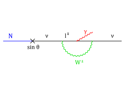
Figure 26: Sterile meutrino decay $N\to\nu_{\alpha}+\gamma$.

If sterile neutrinos are dark matter particles, their decays would produce a narrow line in X-ray flux from cosmos (orbiting velocity of dark matter particles in galaxies is small, $v\lesssim 10^{-3}$, hence the photons produced in their two-body decays are nearly monochromatic). Leaving aside a hint towards 3.5 keV line advocated in Refs. [68, 69] (see the discussion of its status in Ref. [70]), one makes use of strong limits on such a line and translates them into limits on $\sin^{2}\theta$. These limits as function of sterile neutrino mass, are shown in Fig. 27; they rule out the range of masses giving the right mass density of dark matter, eq. (59).

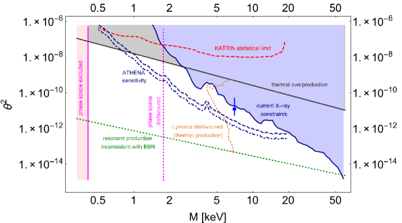
Figure 27: Limits on sterile neutrino parameters (mass $M$, mixing angle squared $\theta^{2}$) obtained from X-ray telescopes [70]. Straight solid line refers to sterile neutrino dark matter produced in non-resonant oscillations, eq. (59). Region between this line and dotted line corresponds to resonant mechanism that works in the Universe with fairly large lepton asymmetry. Vertical lines show very conservative limits coming from phase space and Lyman-$\alpha$ considerations, see Sec. 5.1. Regions left of these lines are disfavored. In fact, for non-resonant mechanism, the phase space constraint is $M\gtrsim 6$ keV. Bullet with vertical interval shows the point corresponding to putative 3.5 keV line.

A (rather baroque) way out [71] is to assume that there is failry large lepton asymmetry in the Universe. Then the oscillations of active neutrino into sterlie neutrino may be enhanced due to the MSW effect, as at some temperature they occur in the Mikheev–Smirnov resonance regime. In that case the right abundance of sterile neutrinos is obtained at smaller $\theta$, and may be consistent with X-ray bounds. This is also shown in Fig. 27.

Direct laboratory searches for strile neutrino are currently sensitive to substantially larger sterile-active mixing angles. This is shown in Fig. 28 and also in Fig. 27, projected KATRIN limit, dashed line.

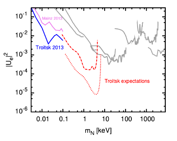
Figure 28: Existing laboratory limits on sterile neutrino mixing with electron neutrino, $|U_{e}|^{2}=\theta_{N\,\nu_{e}}^{2}$, and projected sensitivty of Troitsk nu-mass experiment [72].

9 Dark matter summary

In the first place, the mechanisms discussed here are by no means the only ones capable of producing dark matter, and particles we discussed are by no means the only dark matter candidates. Other dark matter candidates include gravitinos, axinos, Q-balls, very heavy relics produced towards the end of inflation (wimpzillas), primordial black holes, etc. Hence, even though there are grounds to hope that the dark matter problem will be solved soon, there is no guarantee at all. Indeed, some of the candidates, like gravitino or sterile wimpzilla, interact with the Standard Model particles so weakly that their direct discovery is hopeless. Concerning the candidates we have presented, we make a few comments.

• With the exception of axions/ALPs, the plausible candidates are strongly constrained already. However, as we pointed out, this does not mean much, since the actual values of parameters may still be in the unexplored region of the parameter space.

• The null results obtained so far suggest that it makes sense to look for less motivated candidates, and employ diverse search strategies. This happens already: we note in this regard existing and proposed experiments like NA64, SHiP, Troitsk nu-mass, Katrin, etc.

• Astrophysics and cosmology may well provide hints towards the nature of dark matter (CDM vs WDM vs SIMP vs fuzzy DM, etc.)

• WIMPs are attacked from different directions. If dark matter particles are indeed WIMPs, and the relevant energy scale is of order 1 TeV, then the Hot Big Bang theory will be probed experimentally up to temperature of $(\mbox{a~{}few})\cdot(10-100)~{}$GeV and down to age $10^{-9}-10^{-11}~{}$s (compare to 1 MeV and 1 s accessible today through Big Bang Nucleosynthesis). With microscopic physics to be known from collider experiments, the WIMP abundance will be reliably calculated and checked against the data from observational cosmology. Thus, WIMP scenario offers a window to a very early stage of the evolution of the Universe.

• Searches for dark matter axions and ALPs and signal from light sterile neutrino make use of completely different methods. Yet there is good chance for discovery, if either of these particles make dark matter.

All this shows that the situation with dark matter is controversial but extremely interesting.

10 Baryon asymmetry of the Universe

As we discussed in Section 2.6, the baryon asymmetry of the Universe is characterized by the baryon-to-entropy ratio, which at high temperatures is defined as follows,

$$\Delta_{B}=\frac{n_{B}-n_{\bar{B}}}{s}=\frac{1}{3}\frac{n_{q}-n_{\bar{q}}}{s}\;,$$

where $n_{q}$ and $n_{\bar{q}}$ are the number densities of quarks and antiquarks, respectively (baryon number of a quark equals $1/3$), and $s$ is the entropy density. If the baryon number is conserved and the Universe expands adiabatically (which is the case at least after the electroweak epoch, $T\lesssim 100$ GeV), $\Delta_{B}$ is time-independent and equal to its present value $\Delta_{B}\approx 0.86\cdot 10^{-10}$, see eq. (24). At early times, at temperatures well above 100 MeV, cosmic plasma contained many quark-antiquark pairs, whose number density was of the order of the entropy density, $n_{q}+n_{\bar{q}}\sim s$. Hence, in terms of quantities characterizing the very early epoch, the baryon asymmetry may be expressed as

$$\Delta_{B}\sim\frac{n_{q}-n_{\bar{q}}}{n_{q}+n_{\bar{q}}}\;.$$

We see that there was one extra quark per about 10 billion quark-antiquark pairs! It is this tiny excess that is responsible for the entire baryonic matter in the present Universe: as the Universe expanded and cooled down, antiquarks annihilated with quarks, and only the excessive quarks remained and formed baryons.

There is no logical contradiction to suppose that the tiny excess of quarks over antiquarks was built in as an initial condition. This would be very contrived, however. Furthermore, inflationary scenario predicts that the Universe was baryon-symmetric at inflation (no quarks, no antiquarks). Hence, the baryon asymmetry must be explained dynamically [73, 74], by some mechanism of its generation in the early Universe.

10.1 Sakharov conditions

There are three necessary conditions for the generation of the baryon asymmetry from initially baryon-symmetric state. These are Sakharov conditions:

(i) baryon number non-conservation;

(ii) C- and CP-violation;

(iii) deviation from thermal equilibrium.

All three conditions are easily understood. (i) If baryon number were conserved, and initial net baryon number in the Universe vanishes, the Universe today would still be baryon-symmetric. (ii) If C or CP were conserved, then the rate of reactions with particles would be the same as the rate of reactions with antiparticles, and no asymmetry would be generated. (iii) Thermal equilibrium means that the system is stationary (no time-dependence at all). Hence, if the initial baryon number is zero, it is zero forever, unless there are deviations from thermal equilibrium. Furthermore, if there are processes that violate baryon number, and the system approaches thermal equilibrium, then the baryon number tends to be washed out rather than generated (with qualification, see below).

At the epoch of the baryon asymmetry generation, all three Sakharov conditions have to be met simultaneously. There is a qualification, however. These conditions would be literally correct if there were no other relevant quantum numbers that characterize the cosmic medium. In reality, however, lepton numbers also play a role. As we will see shortly, baryon and lepton numbers are rapidly violated by anomalous electroweak processes at temperatures above, roughly, 100 GeV. What is conserved in the Standard Model is the combination $(B-L)$, where $L$ is the total lepton number. So, there are two options. One is to generate the baryon asymmetry at or below the electroweak epoch, $T\lesssim 100$ GeV, and make sure that the electroweak processes do not wash out the baryon asymmetry after its generation. This leads to the idea of electroweak baryogenesis (another possibility is Affleck–Dine baryogenesis [75]). Another is to generate $(B-L)$-asymmetry before the electroweak epoch, i.e., at $T\gg 100$ GeV: if the Universe is $(B-L)$-asymmetric above 100 GeV, the electroweak physics reprocesses $(B-L)$ partially into baryon number and partially into lepton number, so that in thermal equilibrium with conserved $(B-L)$ one has

$$B=C\cdot(B-L)\;,\;\;\;\;\;\;\;L=(C-1)\cdot(B-L)\;,$$ (60)

where $C$ is a constant of order 1 ($C=28/79$ in the Standard Model at $T\gtrsim 100$ GeV). In the second scenario, the first Sakharov condition applies to $(B-L)$ rather than baryon number itself.

There are two most commonly discussed mechanisms of baryon number non-conservation. One emerges in Grand Unified Theories and is due to the exchange of super-massive particles. The scale of these new, baryon number violating interactions is the Grand Unification scale, presumably of order $M_{GUT}\simeq 10^{16}~{}\mbox{GeV}$. It is not very likely, however, that the baryon asymmetry was generated due to this mechanism: the relevant temperature would have to be of order $M_{GUT}$, and so high reheat temperature after inflation is difficult to obtain.

Another mechanism is non-perturbative [38] and is related to the triangle anomaly in the baryonic current (a keyword here is “sphaleron” [76, 77]). It exists already in the Standard Model, and, possibly with mild modifications, operates in all its extensions. The two main features of this mechanism, as applied to the early Universe, is that it is effective over a wide range of temperatures, $100~{}\mbox{GeV}<T<10^{11}~{}\mbox{GeV}$, and, as we pointed out above, that it conserves $(B-L)$. A detailed analysis can be found in the book [78] and in references therein, as well as in lecture notes of similar School [31], and here we only sketch its main ingredients.

10.2 Elecroweak baryon number non-conservation

Let us consider the baryonic current,

$$B^{\mu}=\frac{1}{3}\cdot\sum_{i}\bar{q}_{i}\gamma^{\mu}q_{i}\;,$$

where the sum runs over all quark flavors. Naively, it is conserved, but at the quantum level its divergence is non-zero because of the triangle anomaly (we discussed similar effect in the QCD context in Sec. 7.1; there, the axial current $J_{A}^{\mu}$ is not conserved even in the chiral limit),

$$\partial_{\mu}B^{\mu}=\frac{1}{3}\cdot 3_{colors}\cdot 3_{generations}\cdot\frac{g^{2}}{16\pi^{2}}F^{a}_{\mu\nu}\tilde{F}^{a\,\mu\nu}\;,$$

where $F^{a}_{\mu\nu}$ and $g$ are the field strength of the $SU(2)_{W}$ gauge field and the $SU(2)_{W}$ gauge coupling, respectively, and $\tilde{F}^{a\,\mu\nu}=\frac{1}{2}\epsilon^{\mu\nu\lambda\rho}F^{a}_{\lambda\rho}$ is the dual tensor, cf. eq. (45). Likewise, each leptonic current ($\alpha=e,\mu,\tau$) is anomalous in the Standard Model (we disregard here neutrino masses and mixings, which violate lepton numbers too),

$$\partial_{\mu}L^{\mu}_{\alpha}=\frac{g^{2}}{16\pi^{2}}F^{a}_{\mu\nu}\tilde{F}^{a\,\mu\nu}.$$ (61)

A non-trivial fact is that there exist large field fluctuations, $F^{a}_{\mu\nu}({\bf x},t)\propto g^{-1}$, such that

$$Q\equiv\int~{}d^{3}xdt~{}\frac{g^{2}}{16\pi^{2}}\cdot F^{a}_{\mu\nu}\tilde{F}^{a\,\mu\nu}\neq 0\;.$$ (62)

Furthermore, for any physically relevant fluctuation, the value of $Q$ is integer (“physically relevant” means that the gauge field strength vanishes at infinity in space-time). In four space-time dimensions such fluctuations exist only in non-Abelian gauge theories.

Suppose now that a fluctuation with non-vanishing $Q$ has occured. Then the baryon numbers in the end and beginning of the process are different,

$$B_{fin}-B_{in}=\int~{}d^{3}xdt~{}\partial_{\mu}B^{\mu}=3Q\;.$$ (63)

Likewise

$$L_{\alpha,~{}fin}-L_{\alpha,~{}in}=Q\;.$$ (64)

This explains the selection rule mentioned above: $B$ is violated, $(B-L)\equiv(B-\sum_{\alpha}L_{\alpha})$ is not.

At zero temprature, the field fluctuations that induce baryon and lepton number violation are vacuum fluctuations, called instantons [79]. Since these are large field fluctuations, their probability is exponentially suppressed. The suppression factor in the Standard Model is

$$\mbox{e}^{-{\frac{16\pi^{2}}{g^{2}}}}\sim 10^{-165}\;.$$

Therefore, the rate of baryon number violating processes at zero temperature is totally negligible. On the other hand, at high temperatures there are large thermal fluctuations (“sphalerons”) whose rate is not necessarily small. And, indeed, $B$-violation in the early Universe is rapid as compared to the cosmological expansion at sufficiently high temperatures, provided that (see Ref. [80] for details)

$$\langle\phi\rangle_{T}<T\;,$$ (65)

where $\langle\phi\rangle_{T}$ is the Englert–Brout–Higgs expectation value at temperature $T$.

10.3 Electroweak baryogenesis: what can make it work

Rapid electroweak baryon number non-conservation at high temperatures appears to open up an intriguing possibility that the baryon asymmetry was generated just by these electroweak processes. This should occur at electroweak temperatures, $T_{EW}\sim 100$ GeV, since whatever baryon asymmetry is generated by electroweak processes at higher temperatures, it would be washed out by the same processes as the Universe cools down to $T_{EW}$. There are two obstacles, however:

• CP-violation (2nd Sakharov condition) is too weak in the Standard Model: the CKM mechanism alone is insufficient to generate the realistic value of the baryon asymmetry.

• Departure from thermal equilibrium (3d Sakharov condition) is problematic as well. At temperatures of order $T_{EW}\sim 100$ GeV, the Universe expands very slowly: the cosmological time scale at these temperatures,

  $$H^{-1}(T_{EW})=\frac{M_{Pl}^{*}}{T_{EW}^{2}}\sim 10^{-10}~{}\mbox{s}\;,$$ (66)

  is very large by the electroweak physics standards.

Let us discuss what can make the electroweak mechanism work. We begin with the second obstacle. It appears that the only way to have strong departure from thermal equilibrium at $T_{EW}\sim 100$ GeV is the first order phase transition. Indeed, at temperatures well above 100 GeV electroweak symmetry is restored, and the expectation value of the Englert–Brout–Higgs field $\phi$ is zero, while it is non-zero in vacuo.

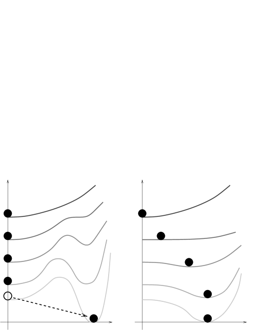
Figure 29: Effective potential as function of $\phi$ at different temperatures. Left: first order phase transition. Right: second order phase transition. Upper curves correspond to higher temperatures. Black blobs show the expectation value of $\phi$ in thermal equilibrium. The arrow in the left panel illustrates the transition from the metastable, supercooled state to the ground state.

This suggests that there may be a phase transition from the phase with $\langle\phi\rangle=0$ to the phase with $\langle\phi\rangle\neq 0$. In fact, the situation is subtle here, as $\phi$ is not gauge invariant, and hence cannot serve as an order parameter, so the notion of phases with $\langle\phi\rangle=0$ and $\langle\phi\rangle\neq 0$ is vague. This is similar to liquid-vapor system, which does not have an order parameter and, depending on pressure, may or may not undergo vapor-liquid phase transition as temperature decreases.

Continuing to use somewhat sloppy terminology, we recall that in thermal equilibrium any system is at the global minimum of its free energy. To figure out the expectation value of $\phi$ at a given temperature, one introduces the temperature-dependent effective potential $V_{eff}(\phi;T)$, which is equal to the free energy density in the system under the constraint that the average field is equal to a prescribed value $\phi$, but otherwise there is thermal equilibrium. Then the global minimum of $V_{eff}$ at given temperature is at the equilibrium value of $\phi$, while local minima correspond to metastable states.

The interesting case for us is the first order phase transition. In this case, the system evolves as follows. At high temperatures, there exists one minimum of $V_{eff}$ at $\phi=0$, and the expectation value of the Englert–Brout–Higgs field is zero. As the temperature decreases, another minimum appears at finite $\phi$, and then becomes lower than the minimum at $\phi=0$, see left panel of Fig. 29. However, the minima with $\phi=0$ and $\phi\neq 0$ are separated by a barrier of $V_{eff}$, the probability of the transition from the phase $\phi=0$ to the phase $\phi\neq 0$ is very small for some time, and the system gets overcooled. The transition occurs when the temperature becomes sufficiently low, and the transition probability sufficiently high. This is to be contrasted to the case, e.g., of the second order phase transition, right panel of Fig. 29. In the latter case, the field slowly evolves, as the temperature decreases, from zero to non-zero vacuum value, and the system remains very close to thermal equilibrium at all times.

The dynamics of the first order phase transition is highly inequilibrium. Thermal fluctuations spontaneously create bubbles of the new phase inside the old phase. These bubbles then grow, their walls eventually collide, and the new phase finally occupies entire space. The Universe boils.In the cosmological context, this process happens when the bubble nucleation rate per Hubble time per Hubble volume is roughly of order 1, i.e., when a few bubbles are created in Hubble volume in Hubble time. The velocity of the bubble wall in the relativistic cosmic plasma is roughly of the order of the speed of light (in fact, it is somewhat smaller, from $0.1$ to $0.01$). Hence, the bubbles grow large before their walls collide: their size at collision is roughly of order of the Hubble size (in fact, one or two orders of magnitude smaller). In other words, the biblles are born microscopic, their initial sizes are determined by the electroweak scale and are roughly of order

$$R_{init}\sim(100~{}\mbox{GeV})^{-1}\sim 10^{-16}~{}\mbox{cm}\;.$$

Their final sizes at the time the bubble walls collide are of order

$$R_{fin}\sim 10^{-2}-10^{-3}~{}\mbox{cm}\;,$$

as follows from (66). One may hope that the baryon asymmetry may be generated during this inequilibrium process.

Does this really happen in the Standard Model? Unfortunately, no: with the Higgs boson mass $m_{H}=125$ GeV, there is no phase transition in the Standard Model at all; there is smooth crossover instead [81].

Nevertheless, the first order phase transition may be characteristic of some extensions of the Standard Model. Generally speaking, one needs the existence of new bosonic fields that have large enough couplings to the Englert–Brout–Higgs field(s). To have an effect on the dynamics of the transition, the new bosons must be present in the cosmic plasma at the transition temperature, $T_{EW}\sim 100$ GeV, so their masses should not be very much higher than $T_{EW}$.

Let us turn to the first obstacle, CP-violation. In the course of the first order phase transition, the baryon asymmetry is generated in the interactions of quarks and leptons with the bubble walls. Therefore, CP-violation must occur at the walls. Now, the walls are made of the scalar field(s), and this points towards the necessity of CP-violation in the scalar sector, which may only be the case in a theory containing scalar fields other than the Standard Model Englert–Brout–Higgs field.

In concrete models with successful electroweak baryogenesis, CP-violation responsible for the baryon asymmetry often leads to sizeable electric dipole moments (EDMs) of neutron and electron. The limits on EDMs are so strong that many such models are actually ruled out. An example is the Non-Minimal Split Supersymmetric Standard Model, which only a few years ago had successfull electroweak baryogenesis [82]. The predictions of this model for electron EDM are shown in Fig. 30. In 2016, when Ref. [82] was written, part of the parameter space was still allowed, but the recent ACME limit [83]

$$d_{e}<1.1\cdot 10^{-29}e\cdot\mbox{cm}$$

rules out the entire parameter space with efficient electroweak baryogenesis.

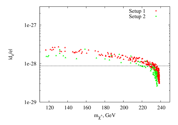
Figure 30: Electron EDM predicted by Non-Minimal Split Supersymmetric Standard Model with parameters suitable for electroweak baryogenesis. Current limit $d_{e}<1.1\cdot 10^{-29}e\cdot\mbox{cm}$ rules out all these models.

To summarize, electroweak baryogenesis requires considerable extension of the Standard Model, often with masses of new particles in the TeV range or lower. Hence, this mechanism will most likely be ruled out or confirmed by the LHC or its successors. Moreover, limits on electron and neutron EDMs make the design of such an extension very difficult. Still, the issue is not decided yet, and the effort to construct the models with successfull electroweak baryogenesis continues [84].

10.4 Baryogenesis in sterile neutrino oscillations

Let us mention another baryogenesis mechanism interesting from the viewpoint of terrestrial experiments, namely, leptogenesis in oscillations of sterile neutrinos [86, 87]. The general idea of leptogenesis [85] is that one or another mechanism generates lepton asymmetry in the Universe before the electroweak transition, and electroweak sphalerons automatically reprocess part of the lepton asymmetry into baryon asymmetry, see eq. (60). The particular version of leptogenesis that we briefly discuss here assumes that there are at least two heavy Majorana neutrinos in the mass range $1-10$ GeV, and that there is strong enough CP-violation in the sterile neutrino sector. Then asymmetries in sterile neutrino sector may be generated and transmitted to active neutrino sector via Yukawa interactions responsible for see-saw masses of acive neutrinos. In the case when there is effectively two sterile neutrino species participating in leptogenesis, correct value of the baryon asymmetry is obtained when the two sterile neutrnos are nearly degenerate,

$$\frac{|M_{1}^{2}-M_{2}^{2}|}{M_{1,2}^{2}}\lesssim 10^{-6}\;,$$

which makes the model rather contrived. However, with three sterile neutrino species, the degeneracy is no longer required [88]. The sterile neutrinos of masses in GeV range and parameters suitable for leptogenesis in their oscillations are typically accessible through rare decays of $B$-mesons, $Z$-bosons, as well as in future beam dump experiments such as SHiP.

An important point concerning this and virtually all other leptogenesis mechanisms is that CP-violation in the sector of active neutrinos, which will hopefully be discovered in oscillation experiments, does not have direct relevance to leptogenesis: the value of lepton, and hence baryon asymmetry is determined by CP-violating parameters in the sterile neutrino sector.

10.5 Baryogenesis summary

We briefly considered here two mechanisms of baryogenesis which may be directly tested, at least in principle, in particle physics experiments. These are certainly not the only mechanisms proposed, and, arguably, not the most plausible mechanisms. One particularly strong competitor is thermal leptogenesis [85], for reviews see, e.g., Ref. [89]. Its idea is that the lepton asymmetry is generated in decays of heavy Majorana sterile neutrinos. The masses of these new particles are well above the experimentally accessible energies. On the one hand, this is in line with the see-saw idea; on the other, direct proof of this mechanism does not appear possible. Interestingly, thermal leptogenesis works only with light active neutrinos: the neutrino masses inferred from cosmology and oscillation experiments are just in the right ballpark.

There are numerous alternative mechanisms of baryogenesis. To name a few, we have already mentioned Affleck–Dine baryogenesis [75]; early discussions concentrated mostly on GUT baryogenesis [90]; there is even a possibility to generate the baryon asymmetry at inflationary epoch [91]. Unfortunately, most of these proposals will be very difficult, if at all possible, to test. So, there is no guarantee at all that we will understand in foreseeable future the origin of matter in the Universe.

11 Before the hot epoch

With Big Bang Nucleosynthesis theory and observations, and due to evidence, albeit indirect, for relic neutrinos, we are confident of the theory of the early Universe at temperatures up to $T\simeq 1$ MeV, which correspond to age of $t\simeq 1$ s. With the LHC, we are learning the Universe up to temperatures $T\sim 100$ GeV and down to age $t\sim 10^{-10}$ s. Are we going to have a handle on even earlier epoch?

Let us summarize the current status of this issue.

• On the one hand, we are confident that the hot cosmological epoch was not the first one; it was preceded by some other, entirely different stage.

• On the other hand, we do not know for sure what was that earlier epoch; an excellent guess is inflation, but alternative scenarios are not ruled out.

• It is conceivable (although not guaranteed) that future cosmological observations will enable us to understand the nature of the pre-hot epoch.

All this makes the situation very interesting. It is fascinating that by studying the Universe at large we may be able to learn about the earliest cosmological epoch which happened at extremely high energy density and expansion rate of our Universe.

11.1 Cosmological perturbations

The key players in this Section are cosmological perturbations. These are inhomogeneities in the energy density and assoiated gravitational potentials, in the first place. It is these inhomogeneites that, among other things, serve as seeds for structures – galaxies, clusters of galaxies, etc. This type of inhomogeneities is called scalar perturbations, as they are described by 3-scalars. There may exist perturbations of another type, called tensor; these are primordial gravity waves. Tensor modes have not been obesrved (yet), so we mostly concentrate on scalar perturbations. While perturbations of the present size of order 10 Mpc and smaller have large amplitudes today and are non-linear, amplitudes of all known perturbations were small in the past, and the linearized theory is applicable. Indeed, CMB temperature anisotropy tells us that the perturbations at recombination epoch were roughly at the level

$$\delta\equiv\frac{\delta\rho}{\rho}=10^{-4}-10^{-5}\;.$$ (67)

We are sloppy here in characterizing the scalar perturbations by the density contrast $\delta\rho/\rho$; we are going to skip technicalities and use this notation in what follows.

Linearized perturbations are most easily studied in momentum space, since the background FLRW metric (1) does not explicitly depend on ${\bf x}$. The spatial Fourier transformation reads

$$\delta({\bf x},t)=\int~{}e^{i{\bf k}{\bf x}}\delta({\bf k},t)~{}d^{3}k\;.$$

Each Fourier mode $\delta({\bf k},t)$ obeys its own linearized equation and hence can be treated separately. Note that the physical distance between neighboring points is $a(t)d{\bf x}$. Thus, ${\bf k}$ is not the physical momentum (wavenumber); the physical momentum is ${\bf k}/a(t)$. While for a given mode the comoving (or coordinate) momentum ${\bf k}$ remains constant in time, the physical momentum gets redshifted as the Universe expands, see also Section 2.1. In what follows we set the present value of the scale factor equal to 1, $a_{0}\equiv a(t_{0})=1$; then ${\bf k}$ is the present physical momentum and $2\pi/k$ is the present physical wavelength, which is also called comoving wavelength.

Properties of scalar perturbations are mesured in various ways. Perturbations of fairly large spatial scales (fairly low ${\bf k}$) give rise to CMB temperature anisotropy and polarization, so we have very detailed knowledge of them. Somewhat shorter wavelengths are studied by analysing distributions of galaxies and quasars at present and in relatively near past. There are several other methods, some of which can probe even shorter wavelengths. There is good overall consistency of the results obtained by different methods, so we have reasonably good understanding of many aspects of the scalar perturbations.

Cosmic medium in our Universe has several components that interact only gravitationally: baryons, photons, neutrinos, dark matter. Hence, there may be and, in fact, there are perturbations in each of these components. As we pointed out in Section 4, electromagnetic interactions between baryons, electrons and photons were strong before recombination, so to reasonable approximation these species made single fluid, and it is appropriate to talk about perturbations in this fluid. After recombination, baryons and photons evolved independently.

11.2 Subhorizon and superhorizon regimes.

It is instructive to compare the wavelength of a perturbation with the horizon size. To this end, recall (see Section 2.6) that the horizon size $l_{H}(t)$ is the size of the largest region which is causally connected by the time $t$, and that

$$l_{H}(t)\sim H^{-1}(t)\sim t$$

at radiation domination and later, see eq. (18). The latter relation, however, holds under assumption that the hot epoch was the first one in cosmology, i.e., that the radiation domination started right after the Big Bang. This assumption is at the heart of what can be called hot Big Bang theory. We will find that this assumption in fact is not valid for our Universe; we are going to see this ad absurdum, so let us stick to the hot Big Bang theory for the time being.

The physical wavelength of a perturbation grows slower than the horizon size. As an example, at radiation domination

$$\lambda(t)=\frac{2\pi a(t)}{k}\propto\sqrt{t}\;,$$

while at matter domination $\lambda(t)\propto t^{2/3}$. For obvious reason, the modes with $\lambda(t)\ll H^{-1}(t)$ and $\lambda(t)\gg H^{-1}(t)$ are called subhorizon and superhorizon at time $t$, respectively. We are interested in the modes which are subhorizon today; longer modes are homogeneous throughout the visible Universe and are not observed. However, the wavelengths which are subhorizon today were superhorizon at some earlier epoch. In other words, the physical momentum $k/a(t)$ was smaller than $H(t)$ at early times; at time $t_{\times}$ such that

$$q(t_{\times})\equiv\frac{k}{a(t_{\times})}=H(t_{\times})\;,$$

the mode entered the horizon, and after that evloved in the subhorizon regime $k/a(t)\gg H(t)$. It is straightforward to see that for all cosmlogically interesting wavelengths, horizon crossing occurs at temperatures below 1 MeV, i.e., at the time we are confident about (repeating the calculation of Sec. 5.1 we find that the present wavelength of order 100 kpc entered the horizon at $T\sim 4$ keV). So, there is no guesswork at this point.

Another way to look at the superhorizon–subhorizon behaviour of perturbations is to introduce a new time coordinate (cf. eq. (16)),

$$\eta=\int_{0}^{t}\frac{dt^{\prime}}{a(t^{\prime})}\;.$$ (68)

Note that this integral converges at lower limit in the hot Big Bang theory. In terms of this time coordinate, the FLRW metric (1) reads

$$ds^{2}=a^{2}(\eta)(d\eta^{2}-d{\bf x}^{2})\;.$$

In coordinates $(\eta,{\bf x})$, the light cones $ds=0$ are the same as in Minkowski space, and $\eta$ is the coordinate size of the horizon, see Fig. 31.

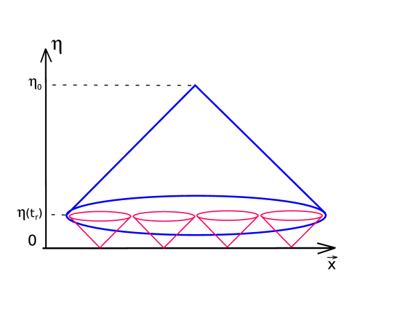
Figure 31: Causal structure of space-time in the hot Big Bang theory. $\eta_{r}$ and $\eta_{0}$ are conformal times at recombination and today, respectively.

Every mode of perturbation has time-independent coordinate wavelength $2\pi/k$, and at small $\eta$ it is in superhorizon regime, $2\pi/k\gg\eta$.

11.3 Hot epoch was not the first

This picture falsifies the hot Big Bang theory. Indeed, within this theory, we see the horizon at recombination $l_{H}(t_{rec})$ at an angle $\Delta\theta\approx 2^{\circ}$, as schematically shown in Fig. 31. By causality, at recombination there should be no perturbations of larger wavelengths, as any perturbation can be generated within the causal light cone only. In other words, CMB temperature must be isotropic when averaged over angular scales exceeding $2^{\circ}$; there should be no cold or warm regions of angular size larger than $2^{\circ}$.

We now take a look at the CMB photographic picture shown in Fig. 2. It is seen by naked eye that there are cold and warm regions whose angular size much exceeds $2^{\circ}$; in fact, there are perturbations of all angular sizes up to those comparable to the entire sky. We come to an important conclusion: the scalar perurbations were built in at the very beginning of the hot epoch, i.e., the cosmological perturbations were generated before the hot epoch.

Another manifestation of the fact that the scalar perturbations were there already at the beginning of the hot epoch is the existence of peaks in the angular spectrum of CMB temperature, as seen in Fig. 3. In general, perturbations in the baryon-photon medium before recombination are acoustic waves (cf. Sec. 4.3),

$$\delta_{B}({\bf k},t)=A({\bf k}){\rm e}^{i{\bf kx}}\cos\left[\int_{0}^{t}~{}v_{s}\frac{k}{a(t^{\prime})}dt^{\prime}+\psi_{\bf k}\right]\;,$$ (69)

where $v_{s}$ is sound speed, $A({\bf k})$ is time-independent amplitude and $\psi_{\bf k}$ is a time-independent phase. This expression is valid, however, in the subhorizon regime only, i.e., at late times. The two solutions in superhorizon regime at radiation domination are

$$\delta_{B}(t) =\mbox{const}\;,$$ (70a)

$$\delta(t)_{B} =\frac{\mbox{const}}{t^{3/2}}\;.$$ (70b)

If the perturbations existed at the very beginning of the hot epoch, they were superhorizon at sufficienly early times, and were described by the solutions (70). The consistency of the whole cosmology requires that the amplitude of perturbations was small at the beginning of the hot stage. The solution (70b) rapidly decays away, and towards the horizon entry the perturbation is in constant mode (70a). So, the initial condition for the further evolution is unique modulo amplitude $A({\bf k})$, and hence the phase $\psi({\bf k})$ is uniquely determined: we have $\psi({\bf k})=0$ for modes entering horizon at radiation domination. As discussed in Sec. 4.3, this leads to oscillatory behavior of baryon-photon perturbations at recombination as function of $k$, and translates into oscillations of CMB temperature multipole $C_{l}$ as function of multipole number $l$.

Were the perturbations generated in a causal way at radiation domination, they would be always subhorizon. In that case the solutions (70) would be irrelevant, and there would be no reason for a particular choice of phase $\psi_{\bf k}$ in eq. (69). One would rather expect that $\psi_{\bf k}$ is a random function of ${\bf k}$, so $\delta_{B}({\bf k},t_{r})$ would not oscillate as function of ${\bf k}$, and oscillations of $C_{l}$ would not exist. This is indeed the case for specific mechanisms of the generation of density perturbations at hot epoch [92].

We conclude that the facts that the CMB angular spectrum has oscillatory behavior and that there are sizeable temperature fluctuations at $l<50$ (angular scale greater than the angular size $2^{\circ}$ of the horizon at recombination) unambiguously tell us that the density perturbations were indeed superhorizon at hot cosmological stage. The hot epoch was preceded by some other epoch — the epoch of the generation of perturbations.

11.4 Inflation or not?

The pre-hot epoch must be long in terms of the time variable $\eta$ introduced in eq. (68). What we would like to have is that the large part of the Universe be causally connected towards the end of that epoch, see Fig. 32.

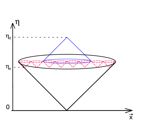
Figure 32: Causal structure of space-time in the real Universe

Long duration in $\eta$ does not necessarity mean long duration in physical time $t$; in fact, the the pre-hot epoch may be very short in physical time.

An excellent hypothesis on the pre-hot stage is inflation, the epoch of nearly exponential expansion [93],

$$a(t)=\mbox{e}^{\int Hdt}\;,\;\;\;\;\;\;\;\;\;H\approx\mbox{const}\;.$$

If this epoch lasts many Hubble times, the whole visible Universe, and likely much greater region of space, is causally connected already at very early times.

From the viewpoint of perturbations, the physical momentum $q(t)=k/a(t)$ decreases (gets redshifted) at inflation, while the Hubble parameter stays almost constant. So, every mode is first subhorizon ($q(t)\gg H(t)$), and later superhorizon ($q(t)\ll H(t)$). This situation is opposite to what happens at radiation and matter domination; this is precisely the pre-requisite for generating the density perturbations. Indeed, inflation does generate primordial density perturbations [94], whose properties are consistent with everything we know about them.

Inflation is not the only hypothesis proposed so far. One alternative option is the bouncing Universe scenario, which assumes that the cosmological evolution begins from contraction, then the contracting stage terminates at some moment of time (bounce) and is followed by expansion. A version is the cycling Universe scenario with many cycles of contraction–bounce–expansion, see Ref. [95] for reviews. Another scenario is that the Universe starts out from nearly flat and static state with nearly vanishing energy density. Then the energy density increases (!), and according to the Friedmann equation, the expansion speeds up. This goes under the name of Genesis scenario [96]. Theoretical realizations of these scenarios are surprizingly difficult, but not impossible, as became clear recently.

12 Towards understanding the earliest epoch

Since cosmological perturbations originate from the earliest epoch that occured before the hot stage, properties of these perturbations will hopefully give us a clue on that epoch. Presently, we know only very basic things about the cosmological perturbations. Let us discuss this point, and at the same time consider promsing directions where further study may lead to breakthrough.

Of course, since the properties we know of are established by observations, thery are valid within certain error bars. Conversely, deviations from the results listed below, if observed, would be extremely interesting.

12.1 Adiabaticity of scalar perturbations

Primordial scalar perturbations are adiabatic. This means that there are perturbations in the energy density, but not in composition. More precisely, the baryon to entropy ratio and dark matter to entropy ratio are constant in space,

$$\delta\left(\frac{n_{B}}{s}\right)=\mbox{const}\;,\;\;\;\;\;\;\delta\left(\frac{n_{DM}}{s}\right)=\mbox{const}\;.$$ (71)

This is consistent with the generation of the baryon asymmetry and dark matter at the hot cosmological epoch: in that case, all partciles were in thermal equilibrium early at the hot epoch, and as long as physics behind the baryon asymmetry and dark matter generation is the same everywhere in the Universe, the baryon and dark matter abundances (relative to the entropy density) are necessarily the same everywhere. In principle, there may exist entropy (or isocurvature) perturbations that violate (one of) the relations (71). No admixture of the entropy perturbations have been detected so far, but it is worth emphasizing that even small admixture will show that many popular mechanisms for generating dark matter and/or baryon asymmetry have nothing to do with reality. One will have to think, instead, that the baryon asymmetry and/or dark matter were generated before the beginning of the hot stage. A notable example is the axion misalignment mechanism discussed in Section 7.

12.2 Gaussianity

The primordial scalar perturbations are Gaussian random field. Gaussianity means that the three-point and all odd correlation functions vanish, while the four-point and higher order even correlation functions are expressed through the two-point function via Wick’s theorem:

$$\langle\delta({\bf k}_{1})\delta({\bf k}_{2})\delta({\bf k}_{3})\rangle = 0$$

$$\langle\delta({\bf k}_{1})\delta({\bf k}_{2})\delta({\bf k}_{3})\delta({\bf k}_{4})\rangle = \langle\delta({\bf k}_{1})\delta({\bf k}_{2})\rangle\cdot\langle\delta({\bf k}_{3})\delta({\bf k}_{4})\rangle$$

$${\ +}~{}{\mbox{permutations~{}of~{}momenta}}\;.$$

We note that this property is characteristic of vacuum fluctuations of non-interacting (linear) quantum fields. Free quantum field has the general form

$$\phi({\bf x},t)=\int d^{3}ke^{-i{\bf kx}}\left(f^{(+)}_{\bf k}(t)a^{\dagger}_{\bf k}+e^{i{\bf kx}}f^{(-)}_{\bf k}(t)a_{\bf k}\right)\;,$$

where $a_{\bf k}^{\dagger}$ and $a_{\bf k}$ are creation and annihilation operators. For the field in Minkowski space-time one has $f^{(\pm)}_{\bf k}(t)=\mbox{e}^{\pm i\omega_{k}t}$, while enhancement, e.g. due to the evolution in time-dependent background, means that $f^{(\pm)}_{\bf k}$ are large. But in any case, Wick’s theorem is valid, provided that the state of the system is vacuum, $a_{\bf k}|0\rangle=0$. Hence, it is quite likely that the density perturbations originate from the enhanced vacuum fluctuations of non-interacting or weakly interacting quantum field(s).

Search for non-Gaussianity is an important topic of current research. It would show up as a deviation from Wick’s theorem. As an example, the three-point function (bispectrum) may be non-vanishing,

$$\langle\delta({\bf k}_{1})\delta({\bf k}_{2})\delta({\bf k}_{3})\rangle=\delta({\bf k}_{1}+{\bf k}_{2}+{\bf k}_{3})~{}G(k_{i}^{2};~{}{\bf k}_{1}{\bf k}_{2};~{}{\bf k}_{1}{\bf k}_{3})\neq 0\;.$$

The functional dependence of $G(k_{i}^{2};~{}{\bf k}_{1}{\bf k}_{2};~{}{\bf k}_{1}{\bf k}_{3})$ on its arguments is different in different models of generation of primordial perturbations, so this shape is a potential discriminator. In some models the bispectrum vanishes, e.g., due to symmetries. In that case the trispectrum (connected 4-point function) may be measurable instead. For the time being, non-Gaussianity has not been detected.

Inflation does the job of producing Gaussian primordial perturbations very well. At inflationary epoch, fluctuations of all light fields get enhanced greatly due to the fast expansion of the Universe. This is true, in particular, for inflaton, the field that dominates the energy density at inflation. Enhanced vacuum fluctuations of the inflaton are reprocessed into adiabatic perturbations in the hot medium after the end of inflation. Inflaton field is very weakly coupled, so the non-Gaussianity in the primordial scalar perturbations is very small [97]. In fact, it is so small that its detection is problematic even in distant future. It is worth noting that this refers to the simplest, single field inflationary models. In models with more than one relevant field the situation may be different, and sizeable non-Gaussianity may be generated.

The generation of the density perturbations is less automatic in scenarios alternative to inflation. Most models proposed so far can be adjusted in such a way that non-Gaussianity is not particularly strong, but potentially observable. In many cases the bispectrum $G(k_{i}^{2};~{}{\bf k}_{1}{\bf k}_{2};~{}{\bf k}_{1}{\bf k}_{3})$ and/or trispectrum are different from inflationary theories.

12.3 Nearly flat power spectrum

Another important property is that the primordial power spectrum of density perturbations is nearly, but not exactly flat. For homogeneous and anisotropic Gaussian random field, the power spectrum completely determines its only characteristic, the two-point function. A convenient definition is

$$\langle\delta({\bf k})\delta({\bf k}^{\prime})\rangle=\frac{1}{4\pi k^{3}}{\cal P}(k)\delta({\bf k}+{\bf k}^{\prime})\;.$$ (72)

The power spectrum ${\cal P}(k)$ defined in this way determines the fluctuation in a logarithmic interval of momenta,

$$\langle\delta^{2}({\bf x})\rangle=\int_{0}^{\infty}~{}\frac{dk}{k}~{}{\cal P}(k)\;.$$

By definition, the flat, scale-invariant spectrum is such that ${\cal P}$ is independent of $k$. The flat spectrum was conjectured by Harrison [98], Zeldovich [99] and Peebles and Yu [100] in the beginning of 1970’s, long before realistic mechanisms of the generation of density perturbations have been proposed.

In view of the approximate flatness, a natural parametrization is

$${\cal P}(k)=A_{s}\left(\frac{k}{k_{*}}\right)^{n_{s}-1}\;,$$ (73)

where $A_{s}$ is the amplitude, $(n_{s}-1)$ is the tilt and $k_{*}$ is a fiducial momentum, chosen at one’s convenience. The flat spectrum in this parametrization has $n_{s}=1$. The cosmological data give [3]

$$n_{s}=0.965\pm 0.004\;.$$ (74)

This quantifies what we mean by nearly, bit not exactly flat power spectrum.

The approximate flatness of the primordial power spectrum in inflationary theory is explained by the symmetry of the de Sitter space-time, which is the space-time of constant Hubble rate,

$$ds^{2}=dt^{2}-\mbox{e}^{2Ht}d{\bf x}^{2}\;,\;\;\;\;\;\;\;\;H=\mbox{const}\;.$$

This metric is invariant under spatial dilatations supplemented by time translations,

$${\bf x}\to\lambda{\bf x}\;,\;\;\;t\to t-\frac{1}{2H}\log\lambda\;.$$

Therefore, all spatial scales are alike, as required for the flat power spectrum. At inflation, $H$ and the inflaton field are almost constant in time, and the de Sitter symmetry is an approximate symmetry. For this reason inflation automatically generates nearly flat power spectrum. However, neither $H$ nor inflaton are exactly time-independent. This naturally leads to the slight tilt in the spectrum. Overall, this picture is qualitatively consistent with the result (74), though quantitative prediction depends on concrete inflationary model.

The situation is not so straightforward in alternatives to inflation: the approximate flatness of the scalar power spectrum is not at all automatic. So, one has to work hard to obtain this property. Similarly to inflationary theory, the flatness of the scalar power spectrum may be due to some symmetry. One candidate symmetry is conformal invariance [101, 102]. The point is that the conformal group includes dilatations, $x^{\mu}\to\lambda x^{\mu}$. This property indicates that the theory possesses no scale, and has good chance for producing the flat spectrum. This idea is indeed realized at least at the toy model level.

12.4 Statistical isotropy.

In principle, the power spectrum of scalar perturbations may depend on the direction of momentum, e.g.,

$${\cal P}({\bf k})={\cal P}_{0}(k)\left(1+w_{ij}(k)\frac{k_{i}k_{j}}{k^{2}}+\dots\right)\;,$$

where $w_{ij}$ is a fundamental tensor in our part of the Universe (odd powers of $k_{i}$ would contradict commutativity of the Gaussian random field $\delta({\bf k})$). Such a dependence would imply that the Universe was anisotropic at the pre-hot stage, when the primordial perturbations were generated. This statistical anisotropy is rather hard to obtain in inflationary models, though it is possible in inflation with strong vector fields [103]. On the other hand, statistical anisotropy is natural in some other scenarios, including conformal models [104]. The statistical anisotropy would show up in correlators [105]

$$\langle a_{lm}a_{l^{\prime}m^{\prime}}\rangle\;\;\;\;\;\;\mbox{with}~{}~{}{l^{\prime}\neq l}~{}~{}\mbox{and/or}~{}~{}{m^{\prime}\neq m}\;.$$

At the moment, the constraints [106] on statistical anisotropy obtained by analysing the CMB data are getting into the region, which is interesting from the viewpoint of some (though not many) models of the pre-hot epoch.

12.5 Tensor modes

The distinguishing property of inflation is the generation of tensor modes (primordial gravity waves) of sizeable amplitude and nearly flat power spectrum. The gravity waves are thus smoking gun for inflation (although there is some debate on this point). Indeed, there seems to be no way of generating nearly flat tensor power spectrum in alternatives to inflation; in fact, most, if not all, alternative scenarios predict unobservably small tensor modes. The reason for their generation at inflation is that the exponential expansion of the Universe enhances vacuum fluctuations of all fields, including the gravitational field itself. Particularly interesting are gravity waves whose present wavelengths are huge, 100 Mpc and larger, and periods are of the order of a billion years and larger. Many inflationary models predict their amplitudes to be very large, of order $10^{-6}$ or so. Shorter gravity waves are generated too, but their amplitudes decay after horizon entry at radiation domination, and today they have much smaller amplitudes making them inaccessible to gravity wave detectors like LIGO/VIRGO, eLISA, etc. A conventional characteristic of the amplitude of primordial gravity waves is the tensor-to-scalar ratio

$$r=\frac{{\cal P}_{T}}{{\cal P}}\;,$$

where ${\cal P}$ is the scalar power spectrum defined in eq. (72) and ${\cal P}_{T}$ is the tensor power spectrum defined in a similar way, but for transverse traceless metric perturbations $h_{ij}$.

Until recently, the most sensitive probe of the tensor perturbations has been the CMB temperature anisotropy [107]. Nowadays, the best tool is the CMB polarization. The point is that a certain class of polarization patterns (called B-mode) is generated by tensor perturbations, while scalar perturbations are unable to create it [108]. Hence, dedicated experiments aiming at measuring the CMB polarization may well discover the tensor perturbations, i.e., relic gravity waves. Needless to say, this would be a profound discovery. To avoid confusion, let us note that the CMB polarization has been already observed, but it belongs to another class of patterns (so called E-mode) and is consistent with the existence of the scalar perturbations only.

The result of the search for effects of the tensor modes on CMB temperature anisotropy is shown in Fig. 33. This search has already ruled out some of the popular inflationary models.

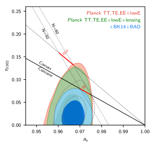
Figure 33: Allowed regions (at 68% and 95% CL) in the plane $(n_{s},r)$, where $n_{s}$ is the scalar spectral index and $r$ is the tensor-to-scalar ratio [3], obtained by Planck collaboration alone and by combining Planck data with BAO data and CMB polarization data from BICEP2/KEK experiments. The right corner (the point $(1.0,0.0)$) is the Harrison–Zeldovich point (flat scalar spectrum, no tensor modes). Intervals show predictions of inflationary models with quadraic and linear inflaton potentials.

13 Conclusion

The present situations in particle physics, on one side, and cosmology, on the other, have much in common. The Standard Model of particle physics and Standard Model of cosmology, $\Lambda$CDM, have been shaped. Both fields enjoyed fairly unexpected discoveries: neutrino oscillations and accelerated expansion of the Universe.

There is strong evidence that the two Standard Models are both incomplete. Therefore, in both fields one hopes for new, revolutionary discoveries. In the context of these lectures, we hope to learn who is dark matter particle; we may learn the origin of matter-antimatter asymmetry in the Universe; the discoveries of new properties of cosmological perturbations will hopefully reveal the nature of the pre-hot epoch.

However, there is no guarantee of new discoveries in particle physics or cosmology. Nature may hide its secrets. Whether or not we will be able to reveal these secrets is the biggest open question in fundamental physics.

References

-
[1]
S. Dodelson, Modern Cosmology, Academic Press, Amsterdam, 2003;
V. Mukhanov, Physical Foundations of Cosmology, Cambridge University Press, 2005;
S. Weinberg, Cosmology, Oxford University Press, 2008;
A. R. Liddle and D.H. Lyth, The Primordial Density Perturbation: Cosmology, Inflation and the Origin of Structure, Cambridge University Press, 2009;
D. S. Gorbunov and V. A. Rubakov, Introduction to the theory of the early universe: Hot big bang theory, 2nd Ed., Hackensack, USA: World Scientific, 2018;
D. S. Gorbunov and V. A. Rubakov, Introduction to the theory of the early universe: Cosmological perturbations and inflationary theory, Hackensack, USA: World Scientific, 2011. - [2] E. Di Valentino, A. Melchiorri and J. Silk, “Planck evidence for a closed Universe and a possible crisis for cosmology,” Nat. Astron. (2019) [arXiv:1911.02087 [astro-ph.CO]].
- [3] N. Aghanim et al. [Planck Collaboration], “Planck 2018 results. VI. Cosmological parameters,” arXiv:1807.06209 [astro-ph.CO].
- [4] Gawiser E. and Silk J. “The Cosmic Microwave Background Radiation,” Phys. Rept. 333 (2000) 245 [ArXiv:astro-ph/0002044].
- [5] N. G. Busca, T. Delubac, J. Rich, S. Bailey, A. Font-Ribera, D. Kirkby, J. M. Le Goff and M. M. Pieri et al., “Baryon Acoustic Oscillations in the Ly- forest of BOSS quasars,” Astron. Astrophys. 552 (2013) A96 [arXiv:1211.2616 [astro-ph.CO]].
- [6] S. Weinberg, “Anthropic Bound on the Cosmological Constant”, Phys. Rev. Lett. 59 (1987) 2607.
- [7] A. D. Linde, “Inflation And Quantum Cosmology”, in: Three hundred years of gravitation. Cambridge Univ. Press, Eds. Hawking, S.W. and Israel, W., 604-630 (1987).
- [8] C. Amsler et al. (Particle Data Group), Phys. Lett. B667 (2008) 1 and 2009 partial update for the 2010 edition.
-
[9]
K. A. Olive,