Towards systematic grid selection in LES:
iterative identification of the coarse-graining length scale by minimizing the solution sensitivity

Abstract

The accuracy of a large eddy simulation (LES) is determined by the accuracy of the model used to describe the effect of unresolved scales, the numerical errors of the resolved scales, and the optimality of the length scale that separates resolved from unresolved scales (the filter-width, or the coarse-graining length scale). This paper is focused entirely on the last of these, proposing a systematic algorithm for identifying the “optimal” spatial distribution of the coarse-graining length scale and its aspect ratio. The core idea is that the “optimal” coarse-graining length scale for LES is the largest length scale for which the LES solution is minimally sensitive to it. This idea is formulated based on an error indicator that measures the sensitivity of the solution and a criterion that determines how that error indicator should vary in space and direction to minimize the overall sensitivity of the solution. The solution to this optimization problem is that the cell-integrated error indicator should be equi-distributed; a corollary is that one cannot link the accuracy in LES to quantities that are not cell-integrated, including the common belief that LES is accurate whenever 80-90% of the energy is resolved. The full method is tested on the wall-resolved LES of turbulent channel flow and the flow over a backward-facing step, with final length scale fields (or filter-width fields, or grids) that are close to what is considered “best practice” in the LES literature. Finally, the derivation of the error indicator offers an alternative explanation for the success of the dynamic procedure.

1 Introduction

Large eddy simulation (LES) is the solution of the Navier-Stokes equations after they have been coarse-grained through some process, whether formally by application of a low-pass filter to the equations or implicitly by discretization on a grid. In either case, one can define a coarse-graining length scale (or filter-width) $\overline{\Delta}$ that separates the resolved from unresolved scales. The effect of the unresolved motions is then modeled, either through an explicitly stated model or implicitly by the numerical error in the discretization. In either case, this process creates a modeling error which scales with the filter-width $\overline{\Delta}$.

The LES equations are solved on a computational grid with a grid-spacing $\overline{h}$, a length scale which controls both the numerical errors and the projection errors [1]. The most common LES approach is to take $\overline{\Delta}=\overline{h}$, in which case the numerical errors are of similar magnitude to the errors caused by the modeling of the unresolved scales [cf. 2, 3]. Some studies have sought “grid-independent LES” by reducing $\overline{h}$ while keeping $\overline{\Delta}$ fixed [cf. 2, 4]; while this produces an LES with negligible numerical errors, it (of course) does not remove the modeling errors, and the resulting LES is necessarily still “filter-width dependent”.

There are two major ways in which the modeling errors in LES can be reduced: (i) by developing models that produce more accurate predictions over a wider range of $\overline{\Delta}$; and/or (ii) by choosing more “optimal” distributions of the filter-width $\overline{\Delta}$. Note that in cases where $\overline{\Delta}=\overline{h}$, the correct choice of $\overline{\Delta}$ would also depend on (and lead to a reduction of) the numerical and projection errors. In most cases, the choice of $\overline{\Delta}$ is arguably at least as important as the subgrid/subfilter model and the numerical implementation. Simply put, provided that the models are consistent (for example behaving consistently near solid walls), most LES codes and subgrid models produce accurate results on sufficiently “good” grids (i.e., filter-width distributions) and inaccurate results on sufficiently “bad” grids. This importance of $\overline{\Delta}$ as a significant modeling parameter stands in some contrast to the literature on LES over the last half century, with many papers published on subgrid modeling (cf. the book by Sagaut [1]) and the influence of numerical errors (cf. [2, 5, 6, 7, 3] and many others), but with few studies devoted to the problem of how to optimally choose $\overline{\Delta}$.

The objective of the present work is to develop a systematic algorithm for finding a nearly “optimal” $\overline{\Delta}$ as a function of both space and direction (i.e., an anisotropic filter-width). This “optimal” distribution, denoted by $\Delta_{\rm opt}({\bf x},{\bf n})$ here (with ${\bf x}$ referring to a spatial location and ${\bf n}$ to a direction), is defined as the coarsest $\overline{\Delta}({\bf x},{\bf n})$ for which the LES solution is still sufficiently accurate. Given the connection between $\overline{\Delta}$ and $\overline{h}$ (since the $\overline{\Delta}/\overline{h}$ ratio is in practice either unity or a fixed predefined value), this work can be viewed equally well as an algorithm for finding the optimal grid.

The optimal filter-width distribution is (of course) flow-dependent, model-dependent, and code-dependent. Since it relies on the LES solution on a given grid, the algorithm is necessarily iterative in nature: as the filter-width (grid) improves between iterations, the estimate of ${\Delta}_{\rm opt}$ becomes more accurate. This type of process is usually termed “grid adaptation”, but could also be called “filter-width adaptation” in the context of LES.

The adaptation process is driven by an “error indicator” that, based on an existing LES solution for a given $\overline{\Delta}({\bf x},{\bf n})$, estimates the characteristics of error generation and leads to a new target $\check{\Delta}({\bf x},{\bf n})$ field that is closer to optimal (by applying some criteria that determines how the error indicator should be distributed). There have been some attempts to develop such error indicators in the literature, most of which have been based on relatively heuristic physics-based arguments.

Some early attempts relied on the importance of the energy dissipation process and thus defined their error indicator as the fraction of energy dissipation caused by the sub-grid/sub-filter scale (SGS/SFS) model to the total [cf. 8]. This is closely related to using the ratio of the eddy viscosity to the molecular viscosity as a measure of accuracy [cf. 9]. However, this general concept is meaningful only at low Reynolds numbers, since the whole idea of LES is to avoid having to resolve the viscous dissipation.

A more successful class of methods was inspired by the more realistic argument that LES is accurate whenever the contribution of the modeled scales to the total kinetic energy is sufficiently small [10]. This is a much better assumption, and more consistent with the purpose and premise of LES. Pope [11] used this intuitive argument to suggest that the proportion of resolved to total kinetic energy could be used as a local indicator function. Bose [12] used the kinetic energy in the smallest resolved scales directly (i.e., without scaling with the resolved or total energy) as an error indicator. In both approaches, $\Delta_{\rm opt}({\bf x},{\bf n})$ was found by requiring a constant and uniform indicator function everywhere in space (e.g., that no more than 10% of the total kinetic energy was in the unresolved/small scales). While this general idea of connecting the accuracy of LES to the amount of small-scale (or unresolved) kinetic energy is quite intuitive and has been found to work well in several cases [12, 13], it is important to acknowledge that it is heuristic in nature: there is no equation showing that error scales with the small-scale or unresolved kinetic energy. For example, a perfect SGS/SFS model used with $\overline{\Delta}/\overline{h}\gg 1$ would introduce no modeling or numerical error regardless of the small-scale kinetic energy. Similarly, while the unresolved kinetic energy (or its ratio to the total) may be a good measure of projection or modeling errors in some of the flows and for some of the variables it may not be true in all flows or for all variables.

Several researchers tried to modify and improve the error indicators discussed so far, or even used the LES solution on more than one grid (usually combined with Richardson extrapolation) to define more accurate indicators [cf. 14, 9, 15, 16, 17], but still based on the same heuristic ideas about the importance of energy or dissipation to LES accuracy. Some of these modified indicators are: the modified “activity parameter” (ratio of dissipations) to include numerical dissipation as well [9, 17], the relative SGS viscosity index [17, 18], the relative Kolmogorov scale index [17, 18], combining the energy-based LES error indicator with another indicator for numerical errors [19], using Richardson extrapolation and the LES solution on two or three grids to better estimate the total kinetic energy [17, 18], etc. Similarly, in the method of Systematic Grid and Model Variation (SGMV), Richardson extrapolation was employed as a way of deconvolution of the mean velocity [14, 15, 17, 20] and Reynolds stresses [20], where in the process the numerical and modeling errors (and their effect on the mean fields) were also approximated.

We should also mention the class of multi-resolution LES (MR-LES) methods [cf. 1, 21] where two parallel simulations are performed on two slightly different grids, with the difference between the two solutions used to infer the sources of error. The chaotic nature of the equations then requires regular synchronization of the two solutions.

The most sophisticated approach to date was developed by Hoffman and Johnsson [cf. 22, 23] and later Barth [24] who defined error indicators within a finite-element framework that included both the numerical errors and the estimated modeling error through a scale-similarity model. They also solved the adjoint equation to directly connect the estimated local errors to integrated “quantities of interest” (QoIs). Despite the comprehensive treatment in these papers, this approach has not been adopted extensively in the community. Part of the reason is probably that the work was focused on the finite-element approach, another is that the adjoint equations diverge exponentially for long-time integration of chaotic flows [cf. 25, 26].

A quantitative comparison of most of the aforementioned error indicators is given in Fig. 1 for the case of the wall-resolved LES of the channel flow.

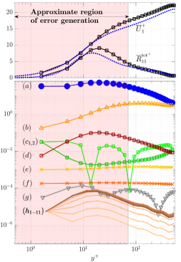
Figure 1: A comparative study of different LES error indicators for a typical wall-resolved LES of the channel flow at $Re_{\tau}\approx 545$ using the Vreman model (constant model coefficient of $c_{v}=0.03$) with a near-wall resolution of $(\overline{\Delta}^{+}_{x},\overline{\Delta}^{+}_{y_{w}}/2,\overline{\Delta}^{+}_{z})\approx(72,2.7,30)$ in friction units, using a sixth-order accurate numerical method and ${\overline{\Delta}}/\overline{h}=1.6$ (to minimize the effect of numerical errors and have a fair comparison between different error indicators). The region of error generation is shaded on both plots. The top panel shows the mean velocity and streamwise Reynolds stress, while the bottom panel plots different error indicators for: $(a)$ the error indicator proposed in this work (defined in Eqn. 7 and converted to a single number in the sense of the integrand of Eqn. 10), $(b)$ ratio of eddy viscosity to molecular viscosity proposed by Geurts and Fröhlich [8], $(c_{1,2})$ ratio of unresolved to total kinetic energy proposed by Pope [11] as “$1-$modified value” proposed by Celik et al. [17] (light green) and the small scale energy normalized by the local value of kinetic energy (dark green), $(d)$ the small-scale energy without local scaling proposed by Bose [12] (also equivalent to the previous work of the present authors [13] applied using a non-directional filter), $(e)$ the ratio of effective viscosity index proposed by Celik et al. [17, 18] ($1-$value), $(f)$ the ratio of Kolmogorov scale index proposed by Celik et al. [17, 18] for the cube root of the cell volume as length scale ($1-$value), $(g)$ sum of the absolute values of the numerical and modeling errors in the mean velocity profile from the SGMV method proposed by Klein et al. [14, 15, 17] for the recommended values of $m=2/3$ (scaling exponent for modeling errors) and $n=6$ (nominal numerical order of accuracy), $(h_{1\mbox{-}11})$ solution error from the MR-LES method proposed by Legrand et al. [21] (lightest to darkest colors correspond to different times after the last synchronization for $(t-t_{s})U_{b}/H=0,\,0.1,\,0.2,\,...,\,1.0$, respectively). The profiles of all error indicators are normalized to make them comparable. Note that the error indicators $(a)$, $(d)$, and $(h)$ are the only successful ones in identifying the region of error generation for this specific flow. Refer to the original text of each work for more details.

One major shortcoming of most existing error indicators is that they are based on scalar error indicators which are unable to infer anything about the optimal anisotropy of $\overline{\Delta}({\bf x},{\bf n})$. In other words, if starting from an isotropic grid/filter-width, a scalar error indicator could never produce an anisotropic final state. This is inconsistent with, for example, the highly anisotropic grids required near the wall in LES. Among the few studies that did address the anisotropy of the filter was that of Addad et al. [27], who defined their $\Delta_{\rm opt}({\bf x},{\bf n})$ directly based on an empirical criterion about the relative size of the filter compared to the Taylor microscale and the RANS dissipation length scale. Another approach was taken by the present authors in prior work [13], where the optimal anisotropy was inferred from the directionally high-pass test-filtered solution field combined with the standard heuristic argument connecting the error generation to the energy in the small-scale field (the filter-width selection criterion of that work was also based on heuristic arguments). The other works that addressed the problem of anisotropy of the grid (cf. [28] as one of the best and most comprehensive examples) had their error indicators defined solely based on the numerical errors and therefore do not fully address the problem in LES.

In the present work we develop a new error indicator for LES that is derived more directly from the governing equation and thus requires less heuristics. The key assumption becomes that the LES equations should be minimally sensitive to a change in the filter-width. The final definition of the error indicator (and in part the reasoning leading to it) becomes closely related to the dynamic procedure [29, 30], and in fact leads to an alternative explanation for why the dynamic procedure works; this is discussed briefly in Section 2.2.

The present work is focused on statistically stationary problems for which we seek a stationary grid/filter-width. In other words, the grid/filter-width is adjusted only between LES runs, and the adaptation step becomes solely a post-processing operation with no changes needed in the LES solver at all. We should also emphasize that the focus here is entirely on the problem of finding $\Delta_{\rm opt}({\bf x},{\bf n})$ and not at all the exact way of creating this new grid (i.e., on the scientific computing aspect, etc.); we simply use currently available tools to generate these grids without worrying about parallel performance, data structures, etc. Other factors like the grid quality, stretching factor, etc. have not been considered either. Consequently, the results presented in this paper could presumably be improved by imposing some constraints on the grid quality metrics or stretching factors, or by use of more sophisticated and flexible grid-generation toolboxes capable of generating a closer grid to the target $\Delta_{\rm opt}({\bf x},{\bf n})$.

2 Methodology

The governing equation for large eddy simulation (LES) can be formally derived by applying a low-pass filter with characteristic filter-width $\overline{\Delta}$ to the Navier-Stokes equation [cf. 31, 1]. In practice, this filtering (or coarse-graining) is often done implicitly when constructing the computational mesh, by assuming that the filter-width is either equal to the grid-spacing $\overline{h}$ or some fixed fraction larger than it. After replacing the unclosed residual stress tensor $\tau_{ij}$ by a model $\tau_{ij}^{\rm mod}(\overline{u}_{k})$, the resulting equation (for incompressible flows) is

$$\frac{\partial\overline{u}_{i}}{\partial t}+\frac{\partial\overline{u}_{i}\overline{u}_{j}}{\partial x_{j}}=-\frac{1}{\rho}\frac{\partial\overline{p}}{\partial x_{i}}+\nu\frac{\partial^{2}\overline{u}_{i}}{\partial x_{j}\partial x_{j}}-\frac{\partial\tau_{ij}^{\rm mod}(\overline{u}_{k})}{\partial x_{j}}\,,$$ (1)

where $\overline{u}_{i}$ and $\overline{p}$ are the resolved velocity and pressure fields, and $\rho$ and $\nu$ are density and kinematic viscosity of the fluid (both assumed constant).

The developments in this paper are based on Eqn. 1 (i.e., for implicitly filtered LES) which is arguably the most popular formulation. Derivations for some alternative forms of this equation are given in B, including: (i) when the convective flux is written as $\overline{\overline{u}_{i}\overline{u}_{j}}$ (used when applying an explicit filter in the solver, known as explicitly filtered LES); (ii) when solving LES without an explicit subgrid model $\tau_{ij}^{\rm mod}$ (implicit LES, or ILES); and (iii) for compressible LES.

2.1 Proposed error indicator

The idea of this section is to estimate how sensitive the LES equation 1 is to a change in the filter-width $\overline{\Delta}$ in any given direction and at any given location, and to use that to define our error indicator. The estimate will be derived and computed using a low-pass test filter, which must be able to filter only in a single direction (i.e., filter modes with high wavenumber in that single direction) in order to infer anything about the anisotropy of the optimal filter-width. On structured grids such a uni-directional test-filter along the grid lines is trivial to implement and there is much flexibility in the choice of test-filter [cf. 1, 32]. To make this work applicable to general geometries and grid topologies, we will instead use the directional differential filter from our previous work [13] defined as

$$\widehat{\overline{\phi}}^{({\bf n}_{0})}\approx\left(I+\frac{\overline{\Delta}_{{\bf n}_{0}}^{2}}{4}{\bf n}_{0}^{T}\nabla\nabla^{T}{\bf n}_{0}\right)\overline{\phi}\,,$$ (2)

where $\overline{\phi}=\overline{\phi}({\bf x})$ is the original resolved LES field, $\widehat{\overline{\phi}}^{({\bf n}_{0})}=\widehat{\overline{\phi}}^{({\bf n}_{0})}\!\!\!\!\!\!({\bf x})$ is the directionally low-pass test-filtered (in direction ${\bf n}_{0}$) field, $\overline{\Delta}_{{\bf n}_{0}}=\overline{\Delta}({\bf x},{\bf n}_{0})$ is the filter-width in direction ${\bf n}_{0}$ (where ${\bf n}_{0}$ is the unit direction vector), and $I$ is the identity tensor (see [33, 34] for the definition of the filter kernel). The doubly contracted Hessian matrix ${\bf n}_{0}^{T}\nabla\nabla^{T}{\bf n}_{0}$ can also be expressed in index notation as $n_{0,i}n_{0,j}\partial^{2}/\partial x_{i}\partial x_{j}=\partial^{2}/\partial x_{({\bf n}_{0})}^{2}$. For a structured grid with uniform grid-spacing and using second-order central differencing the filter of Eqn. 2 simplifies to a uni-directional box filter of width $2\overline{\Delta}({\bf x},{\bf n}_{0})$ applied using the trapezoidal rule. More details about this filter is given in G. Also, note that the chosen test-filter of Eqn. 2 is not unique, but part of a more general class of differential filters [32, 1] that can be modified to contain directional information and potentially replace Eqn. 2.

Applying the directional test-filter to Eqn. 1 yields (assuming that filtering and differentiation commute, see C for how to include the effect of commutation errors, and G for filters with low commutation errors) an evolution equation for the filtered instantaneous fields at the test-filter level as

$$\frac{\partial\widehat{\overline{u}}^{({\bf n}_{0})}_{i}}{\partial t}+\frac{\partial\widehat{\overline{u}_{i}\overline{u}_{j}}^{({\bf n}_{0})}}{\partial x_{j}}=-\frac{1}{\rho}\frac{\partial\widehat{\overline{p}}^{({\bf n}_{0})}}{\partial x_{i}}+\nu\frac{\partial^{2}\widehat{\overline{u}}^{({\bf n}_{0})}_{i}}{\partial x_{j}\partial x_{j}}-\frac{\partial\widehat{\tau_{ij}^{\rm mod}(\overline{u}_{k})}^{({\bf n}_{0})}}{\partial x_{j}}\,.$$ (3)

An alternative way to obtain an evolution equation for the solution at the test-filter level is to write the filtered Navier-Stokes equations (Eqn. 1) at the test-filter level instead:

$$\frac{\partial\widehat{\overline{v}}^{({\bf n}_{0})}_{i}}{\partial t}+\frac{\partial\widehat{\overline{v}}^{({\bf n}_{0})}_{i}\widehat{\overline{v}}^{({\bf n}_{0})}_{j}}{\partial x_{j}}=-\frac{1}{\rho}\frac{\partial\widehat{\overline{q}}^{({\bf n}_{0})}}{\partial x_{i}}+\nu\frac{\partial^{2}\widehat{\overline{v}}^{({\bf n}_{0})}_{i}}{\partial x_{j}\partial x_{j}}-\frac{\partial\tau_{ij}^{\rm mod}\left(\widehat{\overline{v}}^{({\bf n}_{0})}_{k}\right)}{\partial x_{j}}\,,$$ (4)

where $\widehat{\overline{v}}^{({\bf n}_{0})}_{i}$ and $\widehat{\overline{q}}^{({\bf n}_{0})}$ are the resolved velocity and pressure fields at the test-filter level $\widehat{\overline{\Delta}}^{({\bf n}_{0})}\!\!\!\!\!\!=\widehat{\overline{\Delta}}^{({\bf n}_{0})}\!\!\!\!\!\!\!\!({\bf x},{\bf n})$.

Defining the difference between the two solutions as

$$\widehat{\overline{e}}^{({\bf n}_{0})}_{i}=\widehat{\overline{v}}^{({\bf n}_{0})}_{i}-\widehat{\overline{u}}^{({\bf n}_{0})}_{i}\ \ ,\ \ \widehat{\overline{\Pi}}^{({\bf n}_{0})}=\widehat{\overline{q}}^{({\bf n}_{0})}-\widehat{\overline{p}}^{({\bf n}_{0})}\,,$$

and subtracting Eqn. 3 from Eqn. 4 yields an evolution equation for the difference as

$$\underbrace{\frac{\partial\widehat{\overline{e}}^{({\bf n}_{0})}_{i}}{\partial t}+\widehat{\overline{u}}^{({\bf n}_{0})}_{j}\frac{\partial\widehat{\overline{e}}^{({\bf n}_{0})}_{i}}{\partial x_{j}}}_{T_{1}}-\underbrace{\nu\frac{\partial^{2}\widehat{\overline{e}}^{({\bf n}_{0})}_{i}}{\partial x_{j}\partial x_{j}}}_{T_{2}}+\underbrace{\frac{\partial\widehat{\overline{e}}^{({\bf n}_{0})}_{i}\widehat{\overline{e}}^{({\bf n}_{0})}_{j}}{\partial x_{j}}}_{T_{3}}+\underbrace{\widehat{\overline{e}}^{({\bf n}_{0})}_{j}\frac{\partial\widehat{\overline{u}}^{({\bf n}_{0})}_{i}}{\partial x_{j}}}_{T_{4}}+\underbrace{\frac{1}{\rho}\frac{\partial\widehat{\overline{\Pi}}^{({\bf n}_{0})}}{\partial x_{i}}}_{T_{5}}=\widehat{\overline{\mathcal{F}}}^{({\bf n}_{0})}_{i}\,,$$ (5)

where

$$\widehat{\overline{\mathcal{F}}}^{({\bf n}_{0})}_{i}\!\!\!\!\!\!\!({\bf x})=\frac{\partial}{\partial x_{j}}\left(\widehat{\overline{u}_{i}\overline{u}_{j}}^{({\bf n}_{0})}-\widehat{\overline{u}}^{({\bf n}_{0})}_{i}\widehat{\overline{u}}^{({\bf n}_{0})}_{j}\right)+\frac{\partial}{\partial x_{j}}\left(\widehat{\tau_{ij}^{\rm mod}(\overline{u}_{k})}^{({\bf n}_{0})}-\tau_{ij}^{\rm mod}\left(\widehat{\overline{v}}^{({\bf n}_{0})}_{k}\right)\right)\,.$$ (6)

Terms $T_{1}$ and $T_{2}$ in the error evolution equation 5 describe convective and viscous transport, term $T_{3}$ is a nonlinear transport term, term $T_{4}$ becomes a production term in the governing equation of $\widehat{\overline{e}}^{({\bf n}_{0})}_{i}\widehat{\overline{e}}^{({\bf n}_{0})}_{j}$, and term $T_{5}$ is a pressure-like term that keeps $\widehat{\overline{e}}^{({\bf n}_{0})}_{i}$ divergence-free. The terms in Eqn. 5 are grouped such that all terms involving $\widehat{\overline{e}}^{({\bf n}_{0})}_{i}$ are on the left while the terms not involving the error are grouped in $\widehat{\overline{\mathcal{F}}}^{({\bf n}_{0})}_{i}\!\!\!\!\!\!\!({\bf x})$.

The difference $\widehat{\overline{e}}^{({\bf n}_{0})}_{i}$ can be interpreted as a measure of sensitivity of the solution to the filter level used in its computation. In a chaotic system (like LES), this difference will of course diverge exponentially (at early times) and thus rapidly become meaningless when $\widehat{\overline{u}}^{({\bf n}_{0})}_{i}$ and $\widehat{\overline{v}}^{({\bf n}_{0})}_{i}$ become uncorrelated. Having said that, over short time scales, when starting from identical solutions ($\widehat{\overline{e}}^{({\bf n}_{0})}_{i}=0$), Eqn. 5 shows that $\widehat{\overline{\mathcal{F}}}^{({\bf n}_{0})}_{i}\!\!\!\!\!\!\!({\bf x})$ is the source of initial divergence between the two solutions (since, with $\widehat{\overline{e}}^{({\bf n}_{0})}_{i}=0$, all terms of the left side of Eqn. 5 are zero). We can then hypothesize that the magnitude of $\widehat{\overline{\mathcal{F}}}^{({\bf n}_{0})}_{i}\!\!\!\!\!\!\!({\bf x})$ remains a meaningful estimate of the error generation in an LES, even beyond the short time horizon.

The proposed error indicator is then defined as

$$\overline{\mathcal{G}}({\bf x},{\bf n})=\sqrt{\left\langle\widehat{\overline{\mathcal{F}}}^{({\bf n})}_{i}\!\!\!\!\!({\bf x})\,\widehat{\overline{\mathcal{F}}}^{({\bf n})}_{i}\!\!\!\!\!({\bf x})\right\rangle}\,,$$ (7)

where $\left\langle\cdot\right\rangle$ denotes a suitable averaging operator, and $\overline{\cdot}$ signifies the filter-level on which the test-filtering is applied (i.e., $\overline{\Delta}$). In the present work we are interested in finding the optimal static grids for statistically stationary problems, and hence averaging is performed over time and any homogeneous spatial directions. For more general settings the averaging operator could be adjusted accordingly. For example, in flows with strong unsteady effects at a slow time-scale (e.g., vortex shedding) one could use a low-pass time filter, and for temporally periodic flows (e.g., pulsating flows) one could use a phase average.

The final definition of the error indicator given by Eqns. 6 and 7 essentially measures the error in the divergence of the Germano identity tensor. However, rather than heuristically taking this quantity to define an error indicator, the derivations of this section show that this is the relevant quantity to minimize in order to minimize errors related to the filter-width. The connections between the error indicator, the Germano identity, and the dynamic procedure are discussed in more details in Section 2.2.

The first term (the Leonard-like stress) in $\widehat{\overline{\mathcal{F}}}^{({\bf n})}_{i}\!\!\!\!\!({\bf x})$ can be directly computed from the LES solution $\overline{u}_{i}$, and $\tau_{ij}^{\rm mod}(\overline{u}_{k})$ is also known from the LES. On the other hand, the SGS stress tensor in the imagined evolution equation at the test filter level (Eqn. 4) is defined based on the imagined velocity field $\widehat{\overline{v}}^{({\bf n})}_{i}$. One option would be to actually run an additional LES solving Eqn. 4 but in a synchronized way (similar to the MR-LES methods of Legrand et al. [21], but with the error indicator of this work). The alternative, which is applied here, is to use the test-filtered velocity field from the original LES solution to expand the SGS tensor as well, i.e.,

$$\tau^{\rm mod}_{ij}\left(\widehat{\overline{v}}^{({\bf n})}_{k}\right)=\tau^{\rm mod}_{ij}\left(\widehat{\overline{u}}^{({\bf n})}_{k}\right)+\mathcal{T}_{ij}\left(\widehat{\overline{e}}^{({\bf n})}_{k}\right)\,,$$

where the dependence of $\mathcal{T}_{ij}$ on $\widehat{\overline{u}}^{({\bf n})}_{k}$ is purposefully suppressed to emphasize that all of its terms contain $\widehat{\overline{e}}^{({\bf n})}_{k}$ and must vanish when $\widehat{\overline{e}}^{({\bf n})}_{k}=0$ for consistent SGS models (see the supplementary materials for an example of $\mathcal{T}_{ij}$ in the case of Smagorinsky eddy viscosity model). As a result, $T_{6}=\partial\mathcal{T}_{ij}/\partial x_{j}$ can be moved to the left-hand side of Eqn. 5 where it becomes excluded from the imagined error source (based on the same reasoning used before). Note that expanding $\tau^{\rm mod}_{ij}(\widehat{\overline{v}}^{({\bf n})}_{k})$ using the test-filtered field $\widehat{\overline{u}}^{({\bf n})}_{k}$ is not only simpler (and cheaper), but also more consistent with our current formulation.

The Leonard-like stress in the definition of $\widehat{\overline{\mathcal{F}}}^{({\bf n})}_{i}\!\!\!\!\!({\bf x})$ can be further simplified for a known filter kernel. For the example of the filter of Eqn. 2 this term takes the form

$$\widehat{\overline{u}_{i}\overline{u}_{j}}^{({\bf n})}-\widehat{\overline{u}}^{({\bf n})}_{i}\widehat{\overline{u}}^{({\bf n})}_{j}=\frac{{\overline{\Delta}}^{2}_{\bf n}}{2}\frac{\partial\overline{u}_{i}}{\partial x_{({\bf n})}}\frac{\partial\overline{u}_{j}}{\partial x_{({\bf n})}}-\frac{{\overline{\Delta}}^{4}_{\bf n}}{16}\frac{\partial^{2}\overline{u}_{i}}{\partial x_{({\bf n})}^{2}}\frac{\partial^{2}\overline{u}_{j}}{\partial x_{({\bf n})}^{2}}\,,$$ (8)

with no summation over ${\bf n}$. Therefore, the divergence of this term has a second derivative in its leading term and somewhat resembles the truncation or interpolation error of a low-order numerical scheme [cf. 13, 19, 35, 36]. Note that depending on the test-filter (i.e., first, second or higher derivatives in the definition of the differential filter) the Leonard-like stress can generally resemble the truncation error of different numerical schemes. Also note that the leading term in the expansion of Eqn. 8 has a similar form to the Clark model [cf. 1, 37, 38], but with a different coefficient (i.e., $1/2$ instead of $1/12$) due to the difference in filtering.

2.2 Connection to the dynamic procedure

The dynamic procedure [29, 30] is a way to compute model constant(s) through test-filtering, which has received a lot of attention in the LES community. It finds the model coefficient that minimizes

$$\widehat{\overline{e}}_{\rm dyn}=\left\langle(\widehat{\overline{\mathcal{L}}}_{ij}+\widehat{\overline{\mathcal{M}}}_{ij})(\widehat{\overline{\mathcal{L}}}_{ij}+\widehat{\overline{\mathcal{M}}}_{ij})\right\rangle\,,$$

where $\widehat{\cdot}$ is a regular test-filter (i.e., not directional), and

$$\widehat{\overline{\mathcal{L}}}_{ij}=\widehat{\overline{u}_{i}\overline{u}_{j}}-\widehat{\overline{u}}_{i}\widehat{\overline{u}}_{j}\ \ ,\ \ \widehat{\overline{\mathcal{M}}}_{ij}=\widehat{\tau_{ij}^{\rm mod}(\overline{u}_{k})}-\tau_{ij}^{\rm mod}\left(\widehat{\overline{u}}_{k}\right)\,.$$

There have been multiple explanations for how/why the dynamic procedure works. The original explanation appealed to scale similarity in the inertial range (cf. [39, 40] and references therein), but as pointed out by others [cf. 10, 11] this fails to explain why the dynamic procedure works during transition to turbulence or in the near-wall region of turbulent boundary layers (arguably its greatest success). The lack of any scale similarity at the test-filter level in those scenarios (the filter is close to the dissipative range in wall-resolved LES) therefore makes the original explanation unlikely.

Jimenez & Moser [10] suggested that the explanation has to do (among other things) with dissipation, that the dynamic procedure makes the dissipation by the LES model equal to the production of the Leonard stresses. An alternative explanation was put forth by Pope [11], who showed that the dynamic procedure can be derived by requiring that the total Reynolds stress (i.e., resolved plus modeled) should be minimally sensitive to the filtering level, i.e., that the model coefficient should be chosen to minimize (in magnitude)

$$\left(\widehat{\overline{u}_{i}\overline{u}_{j}}+\widehat{\tau_{ij}^{\rm mod}(\overline{u}_{k})}\right)-\left(\widehat{\overline{u}}_{i}\widehat{\overline{u}}_{j}+\tau_{ij}^{\rm mod}(\widehat{\overline{u}}_{k})\right)\,,$$

which is equal to minimizing $\widehat{\overline{\mathcal{L}}}_{ij}+\widehat{\overline{\mathcal{M}}}_{ij}$. Although not directly stated in [11], the choice of the total Reynolds stress as the critical quantity presumably comes from the importance of stresses in momentum transport.

The present derivation of the error indicator $\mathcal{G}$ implies a somewhat similar but slightly different explanation for why the dynamic procedure works, without any specific assumption about turbulence properties like scale-similarity or about the importance of Reynolds stresses, energy or dissipation in the accuracy of the LES solution.

The residual force $\widehat{\overline{\mathcal{F}}}_{i}$ of Eqn. 6 is simply the divergence of the total tensor subject to minimization in the dynamic procedure, i.e.,

$$\widehat{\overline{\mathcal{F}}}_{i}=\frac{\partial}{\partial x_{j}}\left(\widehat{\overline{\mathcal{L}}}_{ij}+\widehat{\overline{\mathcal{M}}}_{ij}\right)\,.$$

Pope arrived at the minimization of this tensor by requiring that the predicted total stress from an LES should be insensitive to the filter level (with a heuristic step that this should lead to a less sensitive, and hence more accurate, solution); here, we instead arrive at the same thing by requiring that the assumed source term in the evolution equation for the difference between the two solutions at the same filter levels (i.e., the solution sensitivity to the filter-width used in its computation) be as small as possible. In other words, while the error in the Germano identity is definitely a relevant quantity in minimizing the solution sensitivity, the significance of the derivation of Section 2.1 is to show that it is the relevant one (and not just one of the relevant measures).

We should also note that the present work clearly suggests that the force $\widehat{\overline{\mathcal{F}}}_{i}$ rather than the tensor $\widehat{\overline{\mathcal{L}}}_{ij}+\widehat{\overline{\mathcal{M}}}_{ij}$ should be minimized in the dynamic procedure. This has actually been tested before in the literature, in the work of Morinishi & Vasilyev [41]. The downside is that this leads to a nonlinear second-order PDE for the model coefficient, which is presumably why this version of the dynamic procedure has not received the attention and popularity it arguably deserved.

Interestingly, our tests on the channel flow suggest that using the full tensor to drive filter-width adaptation leads to extremely fine cells in the wall-normal direction and is therefore strongly discouraged.

2.3 Finding the optimal filter-width

The error indicator estimates the introduction of error into the evolution equation due to insufficient resolution, but does not automatically determine how much the resolution needs to be changed for the error to go down to a certain level. One approach would be to refine the filter by a fixed factor, say cut the filter in half, in any direction ${\bf n}$ and location ${\bf x}$ that the value of the error indicator is above a certain threshold. This is not optimal however. It is much better if we can predict the change of the error indicator for any given change in the filter-width, and then adjust the filter-width proportionally. The latter approach requires a direct link between the error indicator and filter-width (i.e., a model). In the present work, we adopt the simplistic model

$$\check{\mathcal{G}}({\bf x},{\bf n})\approx\overline{g}({\bf x},{\bf n})\check{\Delta}^{\!\alpha}\!({\bf x},{\bf n})\,,$$ (9)

where $\check{\mathcal{G}}({\bf x},{\bf n})$ is the predicted value of the error indicator on the filter-level $\check{\Delta}({\bf x},{\bf n})$ and the “error source density” $\overline{g}({\bf x},{\bf n})$ is computed from the existing LES solution as

$$\overline{g}({\bf x},{\bf n})=\frac{\overline{\mathcal{G}}({\bf x},{\bf n})}{\overline{\Delta}^{\alpha}\!({\bf x},{\bf n})}\,.$$

The exponent $\alpha$ should be different in different flow regimes (free-shear turbulence, near-wall turbulence, etc.; cf. [42]) and in different directions, but is simply taken as $\alpha\!=\!2$ in our assessments on turbulent channel flow (Section 3) and the flow over a backward-facing step (Section 4) without any attempts at finding the best value. The derivations in the rest of this Section are based on a constant value of $\alpha$, with generalization to the spatially and directionally varying scaling exponent given in A.

The optimal filter-width distribution is the one that leads to the highest accuracy among all possible filter distributions with the same computational cost. The “highest accuracy” is considered here to be equivalent to the lowest introduction of “error” in the sense of Eqn. 5. In the following we assume a grid with hexahedral cells, though possibly with “hanging nodes” and not necessarily with a structured topology.

Assuming that the error source is proportional to the magnitude of $\check{\mathcal{G}}$, the total error to be minimized is, for the special case of a grid with only hexahedral cells,

$$\check{e}_{\rm tot}\propto\int_{\Omega}{\sqrt{\check{\mathcal{G}}^{2}({\bf x},{\bf n}_{1})+\check{\mathcal{G}}^{2}({\bf x},{\bf n}_{2})+\check{\mathcal{G}}^{2}({\bf x},{\bf n}_{3})}\ d{\bf x}}\,,$$ (10)

where the ${\bf n}_{1}$, ${\bf n}_{2}$ and ${\bf n}_{3}$ directions are the three directions of the hexahedral cells (or in computational space, for a structured grid). The computational cost is assumed proportional to the number of cells in this work, which can be estimated [cf. 28] as

$$N_{\rm tot}\approx\int_{\Omega}{\frac{d{\bf x}}{\check{{V}}_{c}({\bf x})}}$$

where $\check{{V}}_{c}$ is the volume of a cell. Assuming a fixed ratio of $\overline{\Delta}/\overline{h}$, we then have (again assuming a grid with hexahedral cells)

$$N_{\rm tot}\propto\int_{\Omega}{\frac{d{\bf x}}{\check{\Delta}({\bf x},{\bf n}_{1})\check{\Delta}({\bf x},{\bf n}_{2})\check{\Delta}({\bf x},{\bf n}_{3})}}\,.$$ (11)

These expressions for the total error and the computational cost are simplistic and could of course be made more realistic. For example, the computational cost could include the size of the time step, especially for compressible solvers. One advantage of these simple estimates is that the optimal solution can be found analytically. First, it is quite easy to show that the optimal solution has the error indicator $\check{\mathcal{G}}({\bf x},{\bf n})$ equally distributed among the different directions, i.e., that it is equal in all directions ${\bf n}$ for every fixed location ${\bf x}$ (assuming that $\alpha$ is the same in all directions; see A for more details, including directionally and spatially varying $\alpha$). This can be solved (for the special case of hexahedral cells treated here) to yield

$$\check{\mathcal{G}}_{\rm opt}({\bf x},{\bf n}_{i})=\overline{g}({\bf x},{\bf n}_{i})\check{\Delta}_{\rm opt}^{\alpha}({\bf x},{\bf n}_{i})=\overline{g}_{\rm vol}({\bf x})\check{\Delta}_{\rm vol,opt}^{\alpha}({\bf x})\ ,\ \ i=1,2,3\,,$$ (12)

where

$$\overline{g}_{\rm vol}=\left(\overline{g}({\bf x},{\bf n}_{1})\overline{g}({\bf x},{\bf n}_{2})\overline{g}({\bf x},{\bf n}_{3})\right)^{1/3}\ ,\ \ \check{\Delta}_{\rm vol,opt}=\left(\check{\Delta}_{\rm opt}({\bf x},{\bf n}_{1})\check{\Delta}_{\rm opt}({\bf x},{\bf n}_{2})\check{\Delta}_{\rm opt}({\bf x},{\bf n}_{3})\right)^{1/3}\,.$$

This implies that the predicted optimal cell aspect ratio is, for example,

$$\frac{\check{\Delta}_{\rm opt}({\bf x},{\bf n}_{j})}{\check{\Delta}_{\rm opt}({\bf x},{\bf n}_{1})}=\left(\frac{\overline{g}({\bf x},{\bf n}_{1})}{\overline{g}({\bf x},{\bf n}_{j})}\right)^{1/\alpha}\ ,\ j=2,3\,.$$

Examples of the predicted optimal cell aspect ratios are given in Fig. 2 for a turbulent channel flow and the region inside the recirculation bubble in the flow over a backward-facing step.

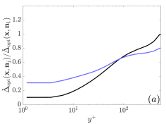
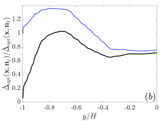
Figure 2: Examples of the predicted optimal cell aspect ratios $\check{\Delta}_{\rm opt}({\bf x},{\bf n}_{2})/\check{\Delta}_{\rm opt}({\bf x},{\bf n}_{1})$ (black lines) and $\check{\Delta}_{\rm opt}({\bf x},{\bf n}_{3})/\check{\Delta}_{\rm opt}({\bf x},{\bf n}_{1})$ (blue lines) for (a) turbulent channel flow and (b) an $x$-normal plane inside the recirculation region of the flow over a backward-facing step ($x/H=2$, see Section 4).

The distribution of $\check{\Delta}_{\rm vol,opt}({\bf x})$ as a function of location ${\bf x}$ can be found by solving an optimization problem that minimizes $\check{e}_{\rm tot}$ of Eqn. 10 with an equality constraint on $N_{\rm tot}$. This reduces to minimizing the Lagrangian $\mathcal{L}=\check{e}_{\rm tot}+\lambda N_{\rm tot}$ (where $\lambda$ is a Lagrange multiplier) with respect to $\check{\Delta}_{\rm vol}({\bf x})$, which for the simplified versions of $\check{e}_{\rm tot}$ and $N_{\rm tot}$ for hexahedral cells takes the solution

$$\overline{g}_{\rm vol}({\bf x})\check{\Delta}_{\rm vol,opt}^{\alpha+3}({\bf x})=\Lambda={\rm const.}$$ (13)

Note that Eqn. 13 clearly suggests that the cell integrated error indicator (i.e., the error indicator, $\overline{g}_{\rm vol}({\bf x})\check{\Delta}_{\rm vol,opt}^{\alpha}({\bf x})$, multiplied by the cell volume, ${\Delta}_{\rm vol,opt}^{3}({\bf x})$) is the quantity that must be uniformly distributed in order to achieve the optimal state. A very important implication of this equation is that the notion of setting quantitative guidelines on the error indicators (e.g., that a good LES is the one that resolves 90% of the total turbulent kinetic energy) is necessarily suboptimal (if not meaningless) and should always be avoided.

Equations 13 and 12 define our optimal filter-width $\check{\Delta}_{\rm opt}({\bf x},{\bf n})$ on any given grid with a specified $N_{tot}$ number of cells.

2.4 The stopping criterion

The question of convergence under grid refinement (or filter-width refinement) can be a bit philosophical in the context of LES. Since LES is by definition under-resolved, the solution will necessarily change and develop smaller scales as one refines the filter-width. So in a point-wise (in space and time) sense, the LES solution does not converge for finer filter-widths, at least not until the DNS limit is reached. While true, this is not a very practical definition of convergence for LES. The National Research Council [43] suggests that the best-practice is to identify important simulation outputs (“quantities of interest”, or QoIs), defined as deterministic functionals of the solution, and assess the convergence of these specific outputs only. This makes sense: if the QoIs we are interested in did not converge well before the DNS limit (in parts of the domain where LES is used), LES would be a pointless tool. In other words, LES makes sense for QoIs that are generally functions of the larger scales of turbulence (e.g., lift, drag, pressure rms, Reynolds stress, etc., that do not directly depend on the fine scales of the solution) but not if the purpose is to predict the fine-scale turbulent quantities (e.g., some short-distance structure function, molecular dissipation or similar, that are functions of the small-scale instantaneous solution). Coming back to the adaptation algorithm, the main point is that (i) the convergence should only be judged for specific QoIs, and not based on whether or not the instantaneous solution is converged, and (ii) this judgement cannot be directly based on the estimated local sources of error; i.e., one cannot assume that the LES is accurate if a certain portion of the turbulence is resolved or if the proposed error indicator is below a certain threshold (even if that threshold in set on the cell integrated error indicator, consistent with Eqn. 13), as that acceptable threshold depends on the flowfield and the specific QoIs.

In principle, the adjoint equation can produce such a link between a QoI and the local error sources, which is why it is possible to estimate the convergence of the QoI in the adjoint-weighted residual method [cf. 44]. However, for a chaotic system like LES the adjoint fields become singular for long time integration [cf. 45, 25, 26] that is required in statistically stationary flows, and the possible workarounds [cf. 25, 26] are still orders of magnitude more expensive than solving the forward LES equation. As a result, we are not considering adjoints in this work. This implies that the proposed adaptation algorithm does not contain a criterion for when to stop the process: this must instead be judged by a user after computing the QoIs and assessing their convergence. Note that once the adjoint equations can be solved the computed adjoint fields can be included in the definition of $\check{e}_{\rm tot}$ in Eqn. 10 (with some minor modifications) to enable a direct link between the estimated local source of errors ($\widehat{\overline{\mathcal{F}}}_{i}^{({\bf n})}\!\!\!\!\!({\bf x})$ in that case) and the error in the QoIs.

Assuming that we have $M$ quantities of interest $\overline{Q}_{m}$ in the simulation allows for the total error in these QoIs to be defined as

$$\overline{e}_{\rm QoI}^{\rm ref}=\sum_{m=1}^{M}{w_{m}\delta\overline{Q}_{m}^{\rm ref}}\,,$$ (14)

where $\delta\overline{Q}_{m}^{\rm ref}$ is the change in $\overline{Q}_{m}$ compared to a reference solution and $w_{m}$ is an appropriate weight with $\sum w_{m}=1$.

Two different reference solutions are used to compute the total error in this paper: (i) the LES solution on the previous grid that was used to compute the error indicator and generate the current grid (labeled $\overline{e}_{\rm QoI}^{\rm prev}$); and (ii) a converged DNS solution (labeled $\overline{e}_{\rm QoI}^{\rm DNS}$). In a practical situation only the former is available, and hence convergence must be judged based on $\overline{e}_{\rm QoI}^{\rm prev}$ alone. The DNS-based error $\overline{e}_{\rm QoI}^{\rm DNS}$ is computed here solely to judge the true accuracy of each solution in order to assess the adaptation process.

The first grid that satisfies the criterion on $\overline{e}_{\rm QoI}^{\rm ref}$ is taken as the “optimal” grid in this work. A more conservative criterion would be to require multiple sequential grids to satisfy the convergence criterion.

The proposed method is next assessed on turbulent channel flow (Section 3) and the flow over a backward-facing step (Section 4).

3 Assessment on turbulent channel flow at $Re_{\tau}\approx 545$

The filter-width adaptation problem is inherently an optimization problem: we should therefore check whether the predicted grids/filter-widths are “optimal”, in the sense of leading to the best accuracy at the lowest cost. While true optimality is extremely difficult to assess in the context of LES (probably impossible, due to the presence of modeling errors and the uncertainties introduced by the projection errors), the turbulent channel flow is arguably as close as we can get given the many decades of experience with this flow in the LES community and the detailed analyses available [cf. 46, 47]. For the turbulent channel cases, we therefore ask whether the adaptation algorithm can produce grids close to the $\Delta_{\rm opt}^{+}\approx(40,1,20)$ or so that is widely considered a “good” grid for wall-resolved LES.

All simulations are started from exceedingly coarse grids that are essentially ignorant of the flow physics; this is done to test the robustness with severely underresolved solutions. In the same spirit, we push the resolution of the final grids to the DNS limit, to make sure that the method is still robust when the LES model becomes effectively inactive. The idea here is that, no matter how coarse or fine the grid might be, a robust method should always drive the grid towards a distribution that leads to lower errors in the solution.

To further test the robustness of the method, we consider three different approaches: (i) LES with a mixture of modeling and numerical errors; (ii) LES where the modeling errors are dominant; and (iii) DNS, which is purely affected by numerical errors.

The predicted filter-widths and associated solution accuracy are compared to those from our previous work [13] in D.

3.1 Code and problem specification

The code used for this problem is the Hybrid code, which solves the compressible Navier-Stokes equations for a calorically perfect gas on structured Cartesian grids using sixth-order accurate central differencing schemes with a split form of the convective term (skew-symmetric in the limit of zero Mach number) for increased numerical stability. Time-integration is handled by classic fourth-order Runge-Kutta. The code solves the implicitly-filtered LES equations with an explicit eddy viscosity model.

The bulk Reynolds number $Re_{b}=\rho_{b}U_{b}H/\mu_{w}$ (where $\rho_{b}$ is the bulk density, $U_{b}$ is the bulk velocity, $H$ is the channel half-height and $\mu_{w}$ is the viscosity at the wall) is 10,000, which leads to a friction Reynolds number of about $Re_{\tau}\approx 545$. The bulk Mach number is 0.2. The computational domains are of size $(L_{x},L_{y},L_{z})=(10H,2H,3H)$. Since the code is structured, the grid-spacing in the wall-parallel directions is taken as the smallest predicted value along $y$. The simulations are integrated for a time of $200H/U_{b}$ (around $11H/u_{\tau}$) before collecting statistics over a period of $600H/U_{b}$ (slightly more than $32H/u_{\tau}$), by post-processing 400 snapshots that are $1.5H/U_{b}$ (close to $0.08H/u_{\tau}$) apart from each other. The convergence error is found to be sufficiently small as to not affect any of the conclusions in this study. This long integration time is primarily required for convergence of the mean profiles, while the adaptation process can actually be performed with averages collected over a much shorter time since the error indicator is primarily affected by small scales. A careful study of the statistical convergence of the error indicator and its predicted grids is delayed until Section 5.

To measure convergence, the QoIs are defined based on the mean velocity and the Reynolds stresses. Specifically, the errors in the QoIs are defined as

$$\delta\overline{Q}_{1}^{{\rm ref}} =\frac{\int_{a}^{b}\left|\overline{U}_{1}^{+}-\widetilde{U}^{+}_{1,{\rm ref}}\right|d\left(\ln y^{+}\right)}{\int_{a}^{b}\widetilde{U}^{+}_{1,{\rm ref}}\,d\left(\ln y^{+}\right)}$$ (15)

$$\delta\overline{Q}_{2\mbox{-}5}^{{\rm ref}} =\frac{\int_{a}^{b}\left|\overline{R}_{ij}^{{\rm tot}^{+}}-\widetilde{R}_{ij,{\rm ref}}^{{\rm tot}^{+}}\right|d\left(\ln y^{+}\right)}{\int_{a}^{b}\widetilde{R}_{kk,{\rm ref}}^{{\rm tot}^{+}}/2\,d\left(\ln y^{+}\right)}\ ,\ \ (i,j)=(1,1),\,(2,2),\,(3,3),\,(1,2)\,.$$

where $\overline{U}_{1}=\left\langle\overline{u}_{1}\right\rangle$ and $\overline{R}^{\rm tot}_{ij}=\left\langle\overline{u}_{i}^{\prime}\overline{u}_{j}^{\prime}\right\rangle+\left\langle\tau_{ij}^{\rm mod}(\overline{u}_{k})\right\rangle$ are the mean velocity and the total Reynolds stress on the LES grid (with characteristic filter-width $\overline{\Delta}$). The reference quantities $\widetilde{U}_{1,{\rm ref}}$ and $\widetilde{R}^{\rm tot}_{ij,{\rm ref}}$ are taken either from the previous LES grid in the sequence of adapted grids (for $\overline{e}_{\rm QoI}^{\rm prev}$) or from the DNS of del Alamo & Jimenez [48] (for $\overline{e}_{\rm QoI}^{\rm DNS}$). The integration limits ($a$ and $b$) are taken as $y^{+}=2$ to $y^{+}=Re_{\tau}/2$ (i.e., $y=H/2$), where the core of the channel is excluded since it is the most affected by the domain size. Note that the error in all of the Reynolds stresses is normalized by the (integral of the) kinetic energy $\widetilde{R}^{{\rm tot}^{+}}_{kk}/2$. These five $\delta\overline{Q}_{m}^{{\rm ref}}$ are then equally weighted to form the final error metric

$$\overline{e}_{\rm QoI}^{\rm ref}=\frac{1}{5}\sum_{m=1}^{5}\delta\overline{Q}_{m}^{{\rm ref}}\,.$$ (16)

3.2 LES with a mixture of modeling and numerical errors

We first use the dynamic Smagorinsky model [29, 30] with filtering and averaging in the wall-parallel directions to compute $\tau_{ij}^{\rm mod}$. Since the implicitly filtered LES equations are solved in the code the filter-width is implicitly assumed to be equal to the grid-spacing, i.e., $\overline{\Delta}/\overline{h}=1$. Combined with the use of numerics with low numerical dissipation, this produces solutions that are contaminated by both modeling and numerical errors of about similar magnitudes [cf. 2, 49].

This first grid has a uniform resolution of $(\overline{\Delta}_{x},\overline{\Delta}_{y},\overline{\Delta}_{z})/H=(0.20,0.10,0.20)$, corresponding to $(\overline{\Delta}_{x}^{+},\overline{\Delta}_{y_{w}}^{+}/2,\overline{\Delta}_{z}^{+})\approx(110,28,110)$ if one uses the fully converged friction velocity. Note that $\overline{\Delta}_{y_{w}}^{+}/2$ is the distance between the first grid point and the wall.

After performing an LES on this grid, we need to compute the error indicator which requires the computation of the eddy viscosity at the test-filter level. Assuming that the model coefficient is the same at the grid- and test-filter levels, this can be computed approximately as

$$\mathcal{V}_{\rm sgs}^{({\bf n}_{0})}\approx\left[\frac{\widehat{\overline{\Delta}}^{({\bf n}_{0})}}{\overline{\Delta}}\!\right]^{\!2}\frac{\left|\widehat{\overline{S}}^{({\bf n}_{0})}\!\right|}{|\overline{S}|}\,\nu_{\rm sgs}\,,$$ (17)

where $\nu_{\rm sgs}$ is the eddy viscosity in the underlying LES. The effect of this approximation is minor, with a full assessment shown in E. We assume $\widehat{\overline{\Delta}}^{({\bf n}_{0})}\!\!\!/\overline{\Delta}\approx\sqrt[3]{2}$ for all 3 directions, since the test-filter of Eqn. 2 is wider by a factor of two in only one direction. This assumes that the characteristic filter-width is taken as the cube-root of the cell volume, which is actually not explicitly enforced here since the filter-width definition can be absorbed into the model constant in the dynamic procedure.

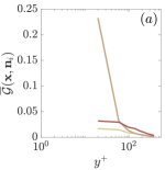
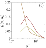
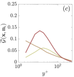
Figure 3: Computed values of $\overline{\mathcal{G}}({\bf x},{\bf n})$ for grids (a) DSM-1, (b) DSM-2 and (c) DSM-3. The streamwise, wall-normal and spanwise directions are shown by the lightest to the darkest colors (in that order).

The computed error indicator on the first grid is plotted in Fig. 3. As expected for this coarse uniform grid, the largest error indicator is for the wall-normal direction in the vicinity of the wall. The next grid (DSM-2) is then generated by enforcing the grid selection criteria of Eqns. 12 and 13. Note that due to the structured nature of the computational grid we have to take the minimum of the target streamwise and spanwise resolutions across the channel in order to generate each of the grids. The constant $\Lambda$ in Eqn. 13 is adjusted (in an iterative process) such that the number of grid points in the next grid DSM-2 increases by a factor of 5.

The key metrics for all grids are reported in Table 1, and the solutions are shown in Fig. 4.

The grid DSM-2 has a grid-spacing of $(\overline{\Delta}_{x}^{+},\overline{\Delta}_{y_{w}}^{+}/2,\overline{\Delta}_{z}^{+})=(77,5.6,55)$. The solution on this grid is actually not bad (Fig. 4), but of course not converged. The error indicator computed from the DSM-2 solution is shown in Fig. 3, and again shows the largest error coming from the wall-normal resolution near the wall, followed by the spanwise resolution throughout much of the buffer layer. The resulting grid DSM-3 produces a solution where the Reynolds stresses are close to the DNS and where the error indicator values in the different directions are closer to being balanced, suggesting that the algorithm has found a nearly “optimal” state.

Grid	$N_{\rm tot}$	$N_{y}$	$(\overline{\Delta}_{x}^{+},\overline{\Delta}_{y_{w}}^{+}/2,\overline{\Delta}_{z}^{+})$	$(\overline{\Delta}_{x},\overline{\Delta}_{y_{c}},\overline{\Delta}_{z})/H$	$Re_{\tau}$	$\overline{e}_{\rm QoI}^{\rm DNS}$ (%)	$\overline{e}_{\rm QoI}^{\rm prev}$ (%)
DSM-1	$15k$	20	$(80,20,80)$	$(0.20,0.10,0.20)$	398	32	$-$
DSM-2	$74k$	34	$(77,5.6,55)$	$(0.14,0.099,0.10)$	553	11	27
DSM-3	$251k$	44	$(53,2.3,29)$	$(0.098,0.091,0.054)$	536	7.3	8.0
DSM-4	$514k$	50	$(45,1.7,19)$	$(0.082,0.080,0.035)$	544	3.3	4.2
DSM-5	$1.18M$	60	$(34,1.4,13)$	$(0.063,0.065,0.024)$	544	1.8	2.1
DSM-6	$2.53M$	72	$(25,1.6,10)$	$(0.046,0.052,0.018)$	542	1.1	1.0
DSM-7	$5.80M$	90	$(18,1.4,7.6)$	$(0.033,0.041,0.014)$	540	1.1	0.6
DSM-8	$11.1M$	108	$(14,1.2,6.3)$	$(0.025,0.033,0.012)$	541	0.9	0.6

Table 1: Sequence of grids generated for LES of channel flow at $Re_{\tau}\approx 545$ using the dynamic Smagorinsky model. $N_{\rm tot}$ is the total number of grid points, while $N_{y}$ denotes the number of points across the channel. $\overline{\Delta}_{\bf n}=\overline{\Delta}({\bf x},{\bf n})$ is both the filter-width and the grid-resolution. Friction resolutions $\overline{\Delta}_{\bf n}^{+}$ are computed based on grid-specific values. $\overline{\Delta}_{y_{w}}^{+}/2$ is distance from the wall of the first grid point. $\overline{\Delta}_{y_{c}}$ is the wall-normal filter-width at the center of the channel. $\overline{e}_{\rm QoI}^{\rm DNS}$ and $\overline{e}_{\rm QoI}^{\rm prev}$ are defined by Eqns. 15 and 16.

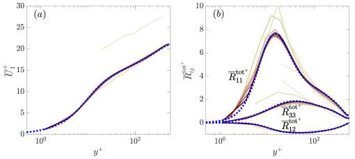
Figure 4: Convergence of the mean velocity and Reynolds stress profiles for the grids in Table 1. Grids in the sequence are shown by the lightest color for DSM-1 to the darkest color for DSM-8. The dotted blue lines show the DNS solution of del Alamo & Jimenez [48] at the same $Re_{\tau}$.

The adaptation algorithm is continued until DSM-8. After the first two adaptations, the target number of cells is doubled each time. The solution is effectively converged on grid DSM-4 or DSM-5 depending on the desired accuracy. The grid-spacings on grids DSM-4 and up are quite close to what is considered “best practice” in LES and DNS for channel flows, with $(\overline{\Delta}_{x}^{+},\overline{\Delta}_{y_{w}}^{+}/2,\overline{\Delta}_{z}^{+})$ of $(45,1.7,19)$ on DSM-4 and $(14,1.2,6.3)$ on DSM-8.

3.3 LES with dominant modeling errors and small numerical errors

The next test case tries to assess the performance of the error indicator in a flow where the numerical errors are relatively small and the solution is mostly dominated by the effect of modeling errors. This is achieved here by taking $\overline{\Delta}/\overline{h}=2$ and using the eddy viscosity model by Vreman [50] with a constant coefficient of $c_{v}=0.03$. The use of a filter-width larger than the grid-spacing causes the eddy viscosity to increase by a factor of 4, which dissipates most of the energy before reaching the Nyquist limit of the grid.

The sequence of grids and solutions are summarized in Table 2 and Fig. 5. The initial grid has the same number of grid points as for the dynamic Smagorinsky case, but twice the filter-width. The subsequent grids in the sequence have approximately the same number of grid points as the corresponding dynamic Smagorinsky cases.

Grid	$N_{\rm tot}$	$N_{y}$	$({\overline{\Delta}}_{x}^{+},\overline{\Delta}_{y_{w}}^{+}/2,{\overline{\Delta}}_{z}^{+})$	$({\overline{\Delta}}_{x},{\overline{\Delta}}_{y_{c}},{\overline{\Delta}}_{z})/H$	$Re_{\tau}$	$\overline{e}_{\rm QoI}^{\rm DNS}$ (%)	$\overline{e}_{\rm QoI}^{\rm prev}$ (%)
Vr-1	$15k$	20	$(153,38,153)$	$(0.40,0.20,0.40)$	382	34	$-$
Vr-2	$73k$	34	$(135,9.5,97)$	$(0.28,0.22,0.20)$	487	21	25
Vr-3	$256k$	44	$(103,4.7,47)$	$(0.21,0.18,0.097$	484	18	7.7
Vr-4	$517k$	50	$(91,4.1,32)$	$(0.18,0.16,0.064)$	500	11	6.0
Vr-5	$1.16M$	62	$(68,3.3,24)$	$(0.13,0.12,0.048)$	510	9.7	2.3
Vr-6	$2.51M$	76	$(49,2.8,20)$	$(0.096,0.096,0.038)$	518	7.1	2.8
Vr-7	$5.83M$	96	$(35,2.3,15)$	$(0.068,0.075,0.029)$	524	5.1	2.1
Vr-8	$11.0M$	114	$(27,1.9,13)$	$(0.052,0.061,0.024)$	530	4.4	1.1

Table 2: Sequence of grids generated for LES of turbulent channel flow using the Vreman model with a model constant of $c_{v}=0.03$ and $\overline{\Delta}/\overline{h}=2$. Additional details on the notation are given in the caption of Table 1. All resolutions are based on the filter-width, not the grid-spacing.

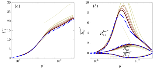
Figure 5: Convergence of the mean velocity and Reynolds stress profiles for grids in Table 2 generated for LES with the constant coefficient Vreman model and $\overline{\Delta}/\overline{h}=2$. Colors vary from the brightest for the first grid to the darkest for the last one. The dotted blue lines are the DNS of del Alamo & Jimenez [48].

The solutions converge much more slowly for this case, which is consistent with the broadly agreed upon notion that for a given grid-spacing $\overline{h}$ the choice of $\overline{\Delta}\approx\overline{h}$ leads to the best LES accuracy in most cases. In other words, that the increase in modeling error for larger filter-widths is greater than the decrease in numerical error.

More interestingly (in the present context) is that the last few grids again agree quite closely with the “best practice” in LES, and in fact agree rather well with the grids for the dynamic Smagorinsky model. For example, grid Vr-5 in Table 2 has a grid-spacing (half the filter-width) of $(34,1.6,12)$ in viscous units, which is almost identical to the resolution of $(34,1.4,13)$ for grid DSM-5 in Table 1.

3.4 DNS affected solely by numerical errors

The final channel case is to turn off the LES subgrid model and thus have only numerical errors. The adaptation algorithm remains the same except that ${\tau}_{ij}^{\rm mod}=0$ in both the solver and when computing the error indicator.

When creating the sequence of grids we target the same number of grid points as in the previous cases. Key metrics are summarized in Table 3 with the convergence of the mean velocity and Reynolds stress profiles shown in Fig. 6.

Grid	$N_{\rm tot}$	$N_{y}$	$({\overline{\Delta}}_{x}^{+},\overline{\Delta}_{y_{w}}^{+}/2,{\overline{\Delta}}_{z}^{+})$	$({\overline{\Delta}}_{x},{\overline{\Delta}}_{y_{c}},{\overline{\Delta}}_{z})/H$	$Re_{\tau}$	$\overline{e}_{\rm QoI}^{\rm DNS}$ (%)	$\overline{e}_{\rm QoI}^{\rm prev}$ (%)
DNS-1	$15k$	20	$(81,20,81)$	$(0.20,0.10,0.20)$	405	30	$-$
DNS-2	$76k$	34	$(80,6.2,56)$	$(0.14,0.094,0.097)$	578	16	24
DNS-3	$252k$	44	$(51,2.4,31)$	$(0.093,0.092,0.057)$	547	6.7	13
DNS-4	$515k$	50	$(43,1.6,22)$	$(0.076,0.086,0.039)$	563	5.0	5.3
DNS-5	$1.14M$	60	$(34,1.6,15)$	$(0.060,0.067,0.026)$	566	4.4	2.2
DNS-6	$2.53M$	72	$(25,1.5,10)$	$(0.046,0.054,0.019)$	553	2.9	2.1
DNS-7	$5.87M$	90	$(18,1.3,7.7)$	$(0.033,0.042,0.014)$	545	1.8	2.4
DNS-8	$11.0M$	106	$(13,1.2,6.4)$	$(0.025,0.034,0.012)$	543	0.9	0.9

Table 3: Sequence of grids generated for DNS of turbulent channel flow at $Re_{\tau}\approx 545$. Additional details on the notation are given in the caption of Table 1.

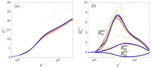
Figure 6: Convergence of the mean velocity and Reynolds stress profiles for grids in Table 3. Colors vary from the brightest for DNS-1 to the darkest for DNS-8. The dotted blue lines show the DNS of del Alamo & Jimenez [48].

The sequence of grids is very similar to those produced for the dynamic Smagorinsky and constant Vreman models in the previous sections. This is partly due to the similarity between wall-resolved LES and DNS grids in wall-bounded turbulence, and partly due to the fact that $\widehat{\overline{\mathcal{F}}}_{i}^{({\bf n})}$ (Eqn. 6) reduces to the divergence of the Leonard-like stress which based on Eqn. 8 resembles a truncation error (although that of a different numerical scheme).

The error in the QoIs is larger for the DNS (no-model) cases than the dynamic Smagorinsky ones, showing that the model has a positive effect for this particular flow and code.

4 Assessment on the flow over a backward facing step at $Re_{H}=5100$

The purpose of this test case is to expose the adaptation algorithm to a more complex flow, with multiple different canonical flow elements: an attached boundary layer upstream of the step, a free shear layer after the separation, an impingement/reattachment region, and a large recirculation zone. This combination of different types of building-block flows is meant to challenge the adaptation algorithm.

The flow geometry and conditions are chosen based on the experiment of Jovic & Driver [51, 52] and the DNS of Le et al. [53]. The computational domain is shown in Fig. 7. The Reynolds number based on the step height $H$ and inflow velocity $U_{\infty}$ is $Re_{H}=U_{\infty}H/\nu=5100$. This corresponds to a momentum Reynolds number of $Re_{\theta}\approx 780$ for the incoming boundary layer (at $x/H=-3$) and a friction Reynolds number of $Re_{\tau}\approx 208$ based on the $\delta_{95}$ boundary layer thickness (or $Re_{\tau}\approx 447$ based on $\delta_{99}$) at that same location. Note that the flow conditions are close to those of the experiment and the DNS, but not exactly the same: the present setup has a thicker boundary layer compared to that of the experiment (which has $Re_{\theta}\approx 610$).

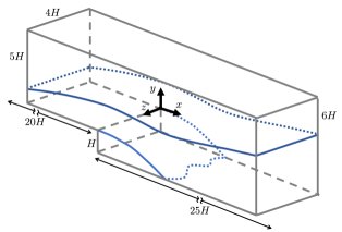
Figure 7: Schematic of the computational domain for the flow over a backward-facing step. The top boundary is a slip wall (modeling the centerline in the experiment) while periodic boundary conditions are used in the spanwise direction. The origin of the coordinate systems is placed at the upper corner of the step.

4.1 Code and computational details

The OpenFOAM code version 2.3.1 [54] is used for this test case to allow for fully unstructured adapted grids. Spatial discretization is done using the linear Gauss scheme (second-order accurate), with second-order backward method for time integration. The pressure-velocity coupling is performed using the PISO algorithm with three iterations of nonorthogonality correction. The filter-width is taken as the cube-root of the cell volume. We use the dynamic $k_{\rm sgs}$-equation model [cf. 55, 56, 57, 58] that defines the eddy viscosity as

$$\nu_{\rm sgs}=c_{k}\overline{\Delta}\sqrt{\overline{k}_{\rm sgs}}$$

and solves a transport equation for $\overline{k}_{\rm sgs}$. This raises the question of how to compute $\widehat{\overline{k}}^{({\bf n}_{0})}_{\rm sgs}$ and thus $\mathcal{V}^{({\bf n}_{0})}$ at the test-filter level. In the present work, we use the simple approach of assuming that the eddy viscosity scales as $\nu_{\rm sgs}\sim\overline{\Delta}^{2}|\overline{S}|$ (a consistency requirement for eddy viscosity models), which then allows us to use the approximate relation (17) to compute the eddy viscosity at the test-filter level. Similar to the channel case, the effect of this approximation is assumed to be small (the assessment is in E). We again take $\widehat{\overline{\Delta}}^{({\bf n}_{0})}\!\!/\overline{\Delta}\approx\sqrt[3]{2}$, which comes from our definition of the characteristic filter-width as the cube root of the cell volume.

The quantities of interest for this flow are taken to be the two non-zero mean velocity components, the four non-zero Reynolds stress components, and the friction and pressure coefficient profiles on the horizontal walls. The errors in the QoIs are defined as

$$\delta\overline{Q}_{1\mbox{-}2}^{\rm ref} =\frac{\int\!\!\int_{\Omega}\left|\overline{U}_{i}-\widetilde{U}_{i,{\rm ref}}\right|dxdy}{0.2U_{\infty}\,A_{\Omega}};\,\,\,\,\,\,i=1,\,2$$

$$\delta\overline{Q}_{3\mbox{-}6}^{{\rm ref}} =\frac{\int\!\!\int_{\Omega}\left|\overline{R}^{\rm tot}_{ij}-\widetilde{R}^{\rm tot}_{ij,{\rm ref}}\right|dxdy}{0.015U_{\infty}^{2}\,A_{\Omega}};\,\,\,\,\,\,(i,j)=(1,1),\,(2,2),\,(3,3),\,(1,2)$$

$$\delta\overline{Q}_{7}^{{\rm ref}} =\frac{\int_{\Psi}\left|\overline{c}_{f}-\widetilde{c}_{f,{\rm ref}}\right|dx}{0.002\,L_{\Psi}};$$

$$\delta\overline{Q}_{8}^{{\rm ref}} =\frac{\int_{\Psi}\left|\overline{c}_{p}-\widetilde{c}_{p,{\rm ref}}\right|dx}{0.1\,L_{\Psi}}\,.$$

where the first two integrals are taken over the region $\Omega\!:\!(x,y)\in[-10H,20H]\times[-H,2H]$, with $A_{\Omega}=10H\!\times\!2H+20H\!\times\!3H$ denoting the area of this region. The remaining two integrals are taken over the horizontal walls in the region $\Psi:x\in[-10H,20H]$ with $L_{\Psi}=30H$ denoting the normalizing length. The quantities are scaled by representative values to make the $\delta\overline{Q}_{m}$ comparable, and then weighted and added together to define the convergence metric as

$$\overline{e}_{\rm QoI}^{{\rm ref}}=\frac{1}{3}\sum_{m=1}^{2}{\frac{\delta\overline{Q}_{m}^{\rm{ref}}}{2}}+\frac{1}{3}\sum_{m=3}^{6}{\frac{\delta\overline{Q}_{m}^{\rm{ref}}}{4}}+\frac{1}{3}\sum_{m=7}^{8}{\frac{\delta\overline{Q}_{m}^{\rm{ref}}}{2}}\,.$$ (18)

Similar to the previous section, we consider both $\overline{e}_{\rm QoI}^{\rm prev}$ defined with respect to the previous grid in the sequence (to judge convergence in a realistic scenario) and $\overline{e}_{\rm QoI}^{\rm DNS}$ defined with respect to a converged DNS (to assess the adaptation method). The reference DNS is computed on a very fine unstructured grid with about 54M cells.

Each case was run for $500H/U_{\infty}$ time units to remove the initial transients, after which 800 snapshots were collected over a period of $2000H/U_{\infty}$. The convergence of the averaging was judged by dividing the full record into four separate batches with 200 snapshots in each, computing the QoIs for each batch, and then computing the sample standard deviation between the batch averages. We then constructed 95% confidence intervals for each quantity using the Student’s t-distribution with 3 degrees of freedom [cf. 59]. The confidence intervals for the integrated errors in the QoIs are very small (and thus omitted below), but they are significant for some of the profiles especially downstream of the step. This is consistent with the expectation of low frequency unsteadiness in the separated flow.

We emphasize that the long averaging times are required only for the solution to converge; the error indicator converges about an order of magnitude more quickly due to its dependence on small scales. The averaging convergence of the error indicator and the resulting predicted grids is investigated in Section 5.

4.2 Results

The initial grid (labeled G-1) has a resolution of $\overline{\Delta}({\bf x},{\bf n})/H=0.2$ everywhere in the domain except close to the walls where the wall-normal direction is refined by a factor of two (we note that the method works equally well without this wall-normal refinement, it just adds another step in the adaptation sequence). After computing the LES on this grid, the error indicator is computed in the three possible directions of refinement/coarsening, and the target filter-width fields for the second grid (G-2) are computed. We then create the actual grid G-2 using the refineMesh utility in OpenFOAM. Since refineMesh can only refine hexahedral cells by factors of 2 in any direction, the resulting grid is different from the predicted target: e.g., a predicted target resolution of $0.17H$ in one location/direction will produce a cell of size $0.10H$ in that location/direction. The resulting grid G-2 (actually, the target filter-width field before creating the refineMesh input) is visualized in Fig. 8. Note that the constant $\Lambda$ in Eqn. 13 was adjusted such that the resulting number of cells was approximately doubled.

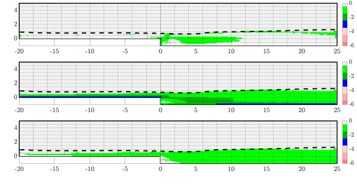
Figure 8: The grid G-2 from Table 4 illustrated by its refinement levels in $x$ (top), $y$ (middle), and $z$ (bottom). Refinement levels are computed based on a skeletal grid with ${\Delta}_{0}({\bf x},{\bf n})=0.2H$ for all ${\bf x}$ and ${\bf n}$. The light green, dark green and blue colors illustrate regions with one ($\overline{\Delta}_{\bf n}/H=0.1$), two ($\overline{\Delta}_{\bf n}/H=0.05$), and three ($\overline{\Delta}_{\bf n}/H=0.025$) refinement levels, respectively. The white regions correspond to areas of the domain that are left untouched (i.e., $\overline{\Delta}_{\bf n}/H=0.2$). The dashed line highlights the $\delta_{95}$ boundary layer thickness.

Figure 8 illustrates how the adaptation methodology targets different regions of the domain for refinement. The algorithm predicts a single level of refinement in the $y$ direction ($\overline{\Delta}({\bf x},{\bf n}_{y})=\overline{\Delta}_{y}=0.1H$) in most of the domain inside the boundary layer, while the $y$ resolution is predicted to need a second level of refinement ($\overline{\Delta}_{y}/H=0.05$) closer to the horizontal walls and in the shear layer, and a third level of refinement ($\overline{\Delta}_{y}/H=0.025$) in close vicinity of the horizontal walls in both incoming and recovering boundary layers. The spanwise resolution $\overline{\Delta}_{z}$ is targeted for a single level of refinement ($\overline{\Delta}_{z}/H=0.1$) for the most part of the domain inside the turbulent boundary layers, while the relaminarized region inside the recirculation bubble is left untouched. The resolution of the skeletal grid in the $x$ direction ($\overline{\Delta}_{x}/H=0.2$) is deemed adequate for the most part of the domain, except near the vertical wall of the step (where the recirculation bubble causes shear) and in the shear layer (where the turbulent fluctuations are significant in all three directions). We also note that the aspect ratio of the cells in the boundary layers and the shear layer are quite close to what we expect from experience for those flows. The fact that the resulting G-2 grid seems this reasonable from an “LES experience” point-of-view is actually quite remarkable, since it was created entirely by an algorithm from a solution on a highly underresolved mesh.

The adaptation process is continued until grid G-7 where the QoIs are deemed converged. Each target grid is generated by aiming for approximately doubling the number of cells, without trying to match this ratio exactly. The sequence of generated grids is reported in Table 4 by their total number of cells $N_{\rm tot}$ and QoI errors (both $\overline{e}_{\rm QoI}^{\rm DNS}$ and $\overline{e}_{\rm QoI}^{\rm prev}$). The Table also reports the grid-spacings in the approaching boundary layer at $x/H=-3$ and shortly after the step at $x/H=1$ (for $y/H=0$) in the shear layer formed by separation at the step. The convergence of the QoIs is shown in Fig. 9 for the pressure and friction coefficients and Figs. 10, 11 and 12 for the mean velocity and Reynolds stress profiles at some of the more interesting locations.

Grid	$N_{\rm tot}$	$(\overline{\Delta}_{x}^{+},\overline{\Delta}_{y_{w}}^{+}/2,\overline{\Delta}_{z}^{+})$	$(\overline{\Delta}_{x},\overline{\Delta}_{y},\overline{\Delta}_{z})/\delta_{\rm shear}$	$\overline{e}_{\rm QoI}^{\rm DNS}$ (%)	$\overline{e}_{\rm QoI}^{\rm prev}$ (%)
G-1	149k	$(42,10,42)$	$(0.21,0.17,0.33)$	11.1	$-$
G-2	297k	$(42,2.6,21)$	$(0.16,0.078,0.16)$	10.5	5.3
G-3	611k	$(45,1.4,11)$	$(0.16,0.049,0.078)$	5.6	6.4
G-4	1.32M	$(47,1.5,12)$	$(0.076,0.038,0.076)$	4.9	3.8
G-5	2.13M	$(25,0.77,6.2)$	$(0.070,0.035,0.035)$	5.4	2.8
G-6	3.41M	$(25,0.77,6.1)$	$(0.068,0.034,0.034)$	3.5	3.4
G-7	6.72M	$(12,0.76.6.0)$	$(0.034,0.017,0.034)$	2.5	2.2
DNS	54M	$(6.0,0.38.3.0)$	$(0.017,0.0086,0.017)$	0	$-$

Table 4: Sequence of grids generated for LES of flow over a backward-facing step. $(\overline{\Delta}_{x}^{+},\overline{\Delta}_{y_{w}}^{+}/2,\overline{\Delta}_{z}^{+})$ correspond to the boundary layer resolutions at $x/H=-3$ upstream of the step, $\delta_{\rm shear}$ is the approximate shear layer thickness at $(x,y)/H=(1,0)$, and $(\overline{\Delta}_{x},\overline{\Delta}_{y},\overline{\Delta}_{z})$ is the resolution at that location. See Fig. 13 for more details. $\overline{e}_{\rm QoI}^{\rm DNS}$ and $\overline{e}_{\rm QoI}^{\rm prev}$ are defined in Eqn. 18.

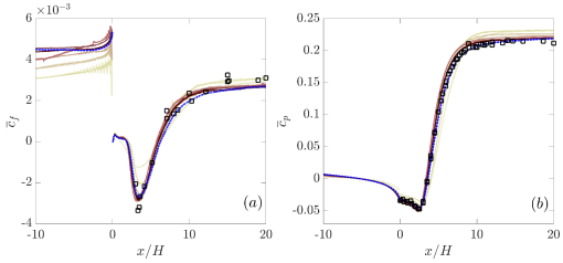
Figure 9: Convergence of (a) friction coefficient $\overline{c}_{f}$ and (b) pressure coefficient $\overline{c}_{p}$ for LES of flow over a backward-facing step. Grids in Table 4 are shown by the lightest color for G-1 to the darkest for G-7. Solid lines denote the sample means, while the shaded regions correspond to the approximate confidence intervals (computed locally). The dotted blue lines and their shaded regions denote our DNS results and their confidence intervals. Symbols correspond to the experimental data of Jovic & Driver [51, 52] with slightly different setup (error bars on the experimental data are not shown). Experimental measurements of $\overline{c}_{f}$ and $\overline{c}_{p}$ are not available upstream of the step.

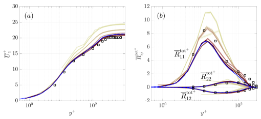
Figure 10: Convergence of the mean velocity and Reynolds stress profiles for the sequence of grids in Table 4 at the incoming boundary layer at $x/H=-3$. Grids in the sequence are shown by the lightest color for G-1 to the darkest for G-7. Solid lines denote the sample means, while the shaded regions correspond to the approximate confidence intervals (computed locally). The dotted blue lines and their shaded regions denote our DNS results and their confidence intervals. Symbols correspond to the experimental data of Jovic & Driver [51, 52] (error bars on the experimental data are not shown).

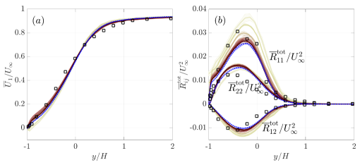
Figure 11: Convergence of the mean velocity and Reynolds stress profles for grids in Table 4 at $x/H=6$ near the reattachment point. See Fig. 10 for more details.

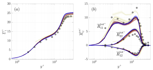
Figure 12: Convergence of the mean velocity and Reynolds stress profiles for the recovering boundary layer at $x/H=15$ for the sequence of grids in Table 4. See Fig. 10 for more details including interpretation of colors.

The computed error $\overline{e}_{\rm QoI}^{\rm DNS}$ decreases after every adaptation except for grid G-5. The relatively large value of the error for this grid is primarily due to the error in the friction coefficient of the incoming boundary layer (see Fig. 9), that happens despite the apparently sufficient resolution of the grid, and affects the entire flowfield downstream of the step.

Figure 13 shows the constructed grid G-6 of Table 4 as an example of a converged LES grid for this specific setup. Note how complicated this grid has become, with many transitions between different grid-resolutions and cells that have completely different aspect ratios from one region of the domain to another (e.g., compare the aspect ratios at the locations reported in Table 4). It is interesting to note how coarse the grid is in the recirculation bubble, expect for the wall-normal directions that are refined to predict the right level of shear at the wall. The most important observation is that these predicted resolutions are very similar to what an experienced user would use when generating a grid for LES of the flow over a backward-facing step.

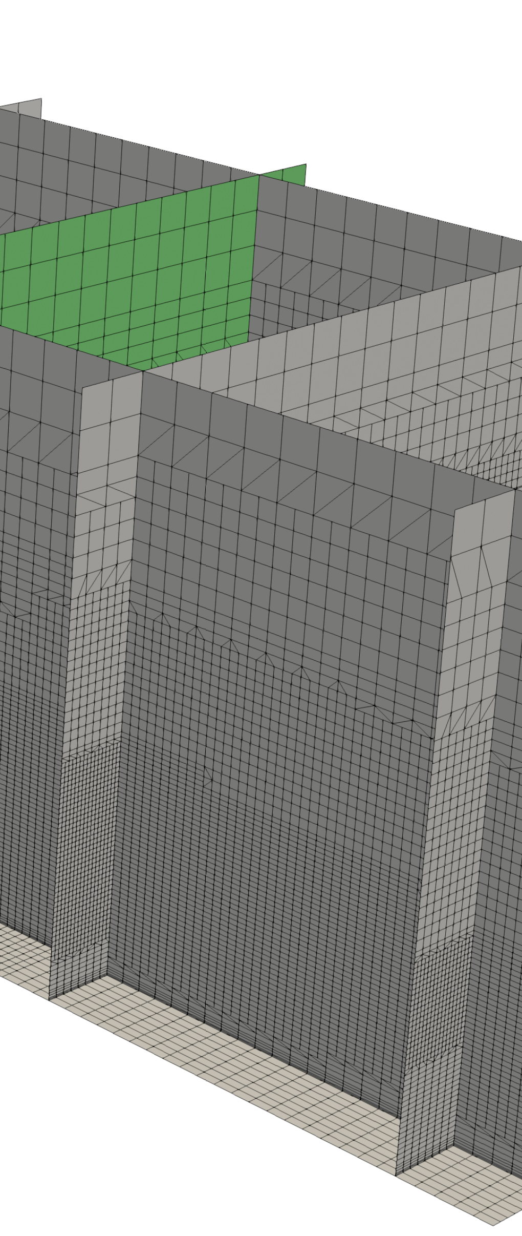
Figure 13: The generated grid G-6 of Table 4 with 3.41M cells. Intersections of the blue planes denote locations whose resolutions are reported in Table 4, while the green planes correspond to $x/H=-3$ and $x/H=6$ whose velocity and Reynolds stress profiles are plotted in Figs. 10 and 11. The grid is resulted from computation of the proposed error indicator (Eqns. 7 and 6) and applying the grid selection criteria of Eqns. 12 and 13 with no user experience involved.

The influence of the initial grid is investigated in F and found to be decreasing for every grid in the sequence with effectively no influence after grid G-4.

5 Statistical convergence of the error indicator and the resulting grid

We conclude by studying the sensitivity of the error indicator and the predicted grids to insufficient averaging in time. Most quantities of interest in LES depend on the large scales of motion which then require a relatively long averaging time for adequate convergence. In contrast, the error indicator depends on the smallest resolved scales and should therefore converge more quickly. The implication is that, in practice, one could reduce the cost of the adaptation process by running only short simulations on many of the grids.

The statistical convergence assessment is done only for the backward-facing step flow, for which we have 800 snapshots spaced $2.5H/U_{\infty}$ apart in time. The error indicator computed using all 800 snapshots is labeled $\overline{\mathcal{G}}_{\rm ref}({\bf x},{\bf n})$, and the refinement level of the resulting grid is labeled $\overline{\mathcal{R}}_{\rm ref}({\bf x},{\bf n})$, where the refinement level is quantified as

$$\overline{\mathcal{R}}({\bf x},{\bf n})=\log_{2}{\frac{\overline{\Delta}({\bf x},{\bf n})}{{\Delta}_{0}({\bf x},{\bf n})}}\,,$$

where ${\Delta}_{0}({\bf x},{\bf n})=0.2$ for all ${\bf x}$ and ${\bf n}$ (this $\overline{\mathcal{R}}({\bf x},{\bf n})$ is what was plotted in Fig. 8).

We also consider averages over batches of $m$ snapshots, for which the resulting error indicator and predicted refinement levels are labeled $\overline{\mathcal{G}}_{m,j}({\bf x},{\bf n})$ and $\overline{\mathcal{R}}_{m,j}({\bf x},{\bf n})$ where $j$ is the batch number. The errors due to insufficient averaging are then defined as

$$\overline{\mathcal{E}}_{\mathcal{G}}(m;j) =\frac{\sum_{i}\int\!\!\int_{\Omega}\left|\overline{\mathcal{G}}_{m,j}({\bf x},{\bf n}_{i})-\overline{\mathcal{G}}_{\rm ref}({\bf x},{\bf n}_{i})\right|d{\bf x}}{\sum_{i}\int\!\!\int_{\Omega}\overline{\mathcal{G}}_{\rm ref}({\bf x},{\bf n}_{i})d{\bf x}}$$ (19)

$$\overline{\mathcal{E}}_{\mathcal{R}}(m;j) =\frac{\sum_{i}\int\!\!\int_{\Omega}\left|\overline{\mathcal{R}}_{m,j}({\bf x},{\bf n}_{i})-\overline{\mathcal{R}}_{\rm ref}({\bf x},{\bf n}_{i})\right|d{\bf x}}{\sum_{i}\int\!\!\int_{\Omega}\left|\overline{\mathcal{R}}_{\rm ref}({\bf x},{\bf n}_{i})\right|d{\bf x}}$$

where $\Omega:{\bf x}=(x,y)\in[-20H,25H]\times[-H,5H]$ is the full two-dimensional domain. This assessment procedure is adopted from our previous work [13], where we also found (by visual comparison) that an error threshold of 0.05 is amply low for both of the errors (for this flow problem and this definition of the error metric). This threshold is therefore used here as well.

Since both $\overline{\mathcal{G}}_{m,j}({\bf x},{\bf n})$ and $\overline{\mathcal{R}}_{m,j}({\bf x},{\bf n})$ are random variables, their errors are also random variables. A 90% two-sided prediction interval is computed for each using the sample mean and sample standard deviation of $\overline{\mathcal{E}}_{\mathcal{G}}(m;j)$ and $\overline{\mathcal{E}}_{\mathcal{R}}(m;j)$ and Student’s t-distribution (cf. [59] for more details on prediction intervals). These prediction intervals are shown in Fig. 14. When the upper bound of the prediction interval lies below the acceptable threshold, there is a 95% chance that the error metric in a single realization is below 0.05. The approximate integration times required for these errors to go below the acceptable threshold are summarized in Table 5.

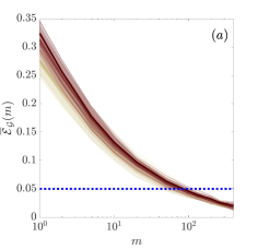
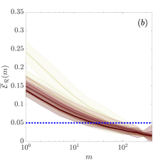
Figure 14: Convergence of (a) the error indicator and (b) the target grids with the number of snapshots $m$ used in the averaging. The grids in Table 4 are shown by the lightest color for G-1 to the darkest for G-7. The solid lines show the sample mean of $\overline{\mathcal{E}}_{\mathcal{G}}(m;j)$ and $\overline{\mathcal{E}}_{\mathcal{R}}(m;j)$ (Eqn. 19), while the shaded regions highlight the $90\%$ prediction interval of the computed values. When the upper bound of the confidence interval goes below the horizontal dotted line there is a 95% chance that the error metric for a single realization is below 0.05.

Grid	$N_{\rm tot}$	$t_{\rm init}U_{\infty}/H$	$t_{\rm QoI}U_{\infty}/H$	$t_{\mathcal{G}}U_{\infty}/H$	$t_{\mathcal{R}}U_{\infty}/H$
G-1	149k	500	2000	260	350
G-2	297k	500	2000	240	220
G-3	611k	500	2000	190	90
G-4	1.32M	500	2000	200	120
G-5	2.13M	500	2000	300	330
G-6	3.41M	500	2000	220	150
G-7	6.72M	500	2000	260	110

Table 5: Comparison of the simulation run times used for removing the initial transients (denoted by $t_{\rm init}$) and computing accurate mean QoI profiles (denoted by $t_{\rm QoI}$) with the integration times required for accurate computation of the error indicator ($t_{\mathcal{G}}$) and the refinement levels of the next optimal grid ($t_{\mathcal{R}}$). For regular situations (i.e., where the flowfield does not undergo a bifurcation) the required integration time to remove the initial transients is presumably shorter for the error indicator and the target grids compared to the QoIs; however, it has not been investigated in this section.

It is quite clear from Fig. 14 and Table 5 that the proposed error indicator and its predicted grids require almost one order of magnitude shorter integration times compared to what is needed for sufficiently converged QoI profiles (once the transients are gone). In other words, we only need to collect $m\lesssim 120$ snapshots (equivalent to an integration time of $\lesssim 300H/U_{\infty}$) to compute sufficiently accurate values of the error indicator, and the required integration time is similar on all grids. The error in the target grids show a very similar behavior in general: grids G-3 to G-7 only require an integration time of $\lesssim 150H/U_{\infty}$ (interestingly, grid G-5 is an outlier here as well, requiring an integration time of $330H/U_{\infty}$).

Note that the initial transient must of course be removed, a time which is highly flow specific; for the cases studied here, the initial transient was about 500 time units.

Finally, we emphasize that although the exact results presented here are specific to the flow over a backward-facing step, the sampling frequency, and other flow parameters, the conclusion about a much faster convergence of the error indicator and target grids compared to the QoIs is probably more general and valid for a broader set of flows.

6 Summary, discussion and future directions

The goal of this paper has been to introduce a systematic approach to finding the “optimal” filter-width distribution (or, equivalently, the “optimal” grid) for large eddy simulation (LES). The long-term vision is to (i) reduce the amount of human time spent on grid-generation (by automating the process), (ii) reduce the computational time (by producing more “optimal” grids), and (iii) make the LES simulation process more systematic (e.g., so different users/codes produce more similar results).

The heart of the proposed adaptation algorithm is the error indicator $\overline{\mathcal{G}}({\bf x},{\bf n})$ defined in Eqn. 7, which estimates the error introduced into the LES evolution equation at location ${\bf x}$ caused by an insufficient filter-width in direction ${\bf n}$. More specifically, the error indicator measures the initial divergence between the test-filtered LES solution and an imagined solution to the test-filtered LES equation. In other words, it measures how sensitive the LES equation is to small (directional) changes in the filter-width. While the error indicator is based on manipulations of the governing equation, it is also based on the assumption that the source of initial divergence between these different solutions is a meaningful measure of the error in the fully nonlinear long-time evolution of the LES. This is really the key physical assumption in this work.

The “optimal” filter-width is found by equi-distribution of the cell integrated error indicator (i.e., the value of the error indicator multiplied by the cell volume, to second order accuracy). While this was the solution to the optimization problem for the error indicator of this work (Section 2.3), it appears to hold for many of the other error indicators; generally speaking, if the value of the error indicator is assumed to be proportional to the local error generation, the overall error is proportional to the volume integral of the local value, for which the optimization problem takes the same solution of equi-distribution of the cell integrated value. This suggests that the popular approach of setting a threshold on the error indicator itself, e.g., judging the accuracy of LES by the ratio of unresolved to total turbulent kinetic energy, is at best suboptimal (if not wrong) and should be avoided.

The adaptation process is tested on a channel flow and the flow over a backward-facing step. For the channel, the algorithm consistently produces grids/filter-widths that are very close to what is considered “best practice” in LES and DNS: grids with $(\overline{\Delta}_{x}^{+},\overline{\Delta}_{y_{w}}^{+}/2,\overline{\Delta}_{z}^{+})\approx(45,1.7,19)$ and $(13,1.2,6.4)$, respectively. For the backward-facing step, the predicted grids are close to what an experienced user might produce. It is essentially impossible to say how “optimal” (in the mathematical sense) the grids are for this problem, but we note that the error (compared to DNS) reaches about 5% with only 600K to 2M cells; it is hard to imagine an experienced user creating a better grid than that (note that the code uses a low-order numerical scheme), at least without significant trial-and-error.

The subgrid/subfilter model used in the LES solution enters directly into the definition of the residual forcing term and thus the error indicator. This is theoretically advantageous, since a more accurate subfilter model would produce a lower error indicator for the same resolved velocity field.

We also note that the proposed error indicator has similarities with the dynamic procedure but was derived without any appeals to scale-similarity in the inertial subrange of turbulence. Its use is not restricted to filter-widths in the inertial subrange, and the derivation in fact offers an alternative explanation for the success of the dynamic procedure.

The error indicator was derived for the incompressible Navier-Stokes equation in this paper, but can be easily extended to other physics. A derivation for compressible flow is shown in B, which creates a separate error indicator for the energy equation. Following the same process, one could extend it to chemically reacting flows, etc.

6.1 Cost

One potential criticism of this type of adaptation algorithm is the additional cost of performing LES on a full sequence of grids. We make four counter-arguments and observations.

First, assuming that the cell count is doubled at each iteration and that the time step scales as $N_{\rm tot}^{1/3}$, the total cost of computing all grids in the sequence (including the final one) is $\lesssim 1.66N_{\rm final}$. If the cell count is quadrupled at each iteration, the total cost is $\lesssim 1.19N_{\rm final}$ instead.

Second, one could start from a “best guess” grid in practice (based on prior experience with the flow in question), thus reducing the number of steps of the algorithm. We only started from exceedingly coarse and “ignorant” initial grids here in order to test the robustness of the method.

Third, as shown in Section 5, the error indicator converges faster (in terms of integration time) than the LES itself due to its dependence on the smallest resolved scales. Therefore, one could run the simulations on the first several grids for shorter times.

Finally, the minor added computational cost must of course be balanced against the larger cost saving of having a more “optimal” final grid. This saving will presumably become larger for more complex flow problems.

6.2 Possible future directions

The present error indicator was derived for the continuous governing equation and as such does not directly estimate any numerical errors (despite the similarity of the Leonard-like stress to the truncation error). The adaptation algorithm was still found to perform well for the DNS of channel flow (which has only numerical errors), but it may be required to explicitly include the numerical errors in the error indicator in other flows.

We also note that the error indicator arguably measures the sensitivity of the solution at the test-filter level and not at the LES filter level $\overline{\Delta}$. This is perfectly fine (perhaps even desirable) for the final grid(s), but may not be ideal for the initial grids in the sequence that are far from resolving the inertial subrange of the turbulence. One possibility is to investigate approaches similar to that of Porte-Agel et al. [60] who revised the dynamic procedure to work better on underresolved grids.

Throughout this work we assumed a constant scaling exponent of $\alpha({\bf x},{\bf n})=2$ for all ${\bf x}$ and ${\bf n}$. In A we show that a spatially/directionally varying exponent $\alpha$ changes the grid selection criterion, in terms of both the aspect ratio and the spatial distribution. This may become important when $\alpha$ is dramatically different in different directions (e.g., in codes where only the spanwise direction is handled by the Fourier expansion) or in different locations. A possible improvement of the method could be achieved by either using the theoretical values of $\alpha$ in different directions (if they are known), or to add a second level of test-filtering to estimate $\alpha({\bf x},{\bf n})$ as well.

There are also several possibilities to improve the grid selection criteria used to generate the grids. For compressible solvers with explicit time-stepping, it may be important to include the number of time steps in the estimated computational cost. This would then effectively “penalize” very thin cells near boundaries. More generally, since it is well known that numerical and commutation errors are highly sensitive to the smoothness of the mesh, one should certainly include a penalization of too rapid filter-width transitions when solving the optimization problem.

A major improvement would be to include the adjoint of the quantity of interest (QoI) and thus make the adaptation “output-based”. This has been the major advancement in steady-state grid-adaptation over the last few decades [cf. 44]. Inclusion of the adjoint would first require the problem of exponential divergence of the adjoint for chaotic problems to be solved [cf. 45].

Appendix A Directionally and spatially varying grid scaling exponent $\alpha$ and how it changes the grid selection criterion

The grid scaling exponent $\alpha$ in the model $\check{\mathcal{G}}({\bf x},{\bf n})\approx\overline{g}({\bf x},{\bf n})\check{\Delta}^{\alpha}({\bf x},{\bf n})$ is in general a function of both space ${\bf x}$ and direction ${\bf n}$, i.e., $\alpha=\alpha({\bf x},{\bf n})$. If we follow the same approach used in Section 2.3, but allow for spatially and directionally varying $\alpha$, the solution to the optimization problem can be obtained by minimizing the Lagrangian

$$\mathcal{L} =\int_{\Omega}{\left(\sqrt{\check{\mathcal{G}}^{2}({\bf x},{\bf n}_{1})+\check{\mathcal{G}}^{2}({\bf x},{\bf n}_{2})+\check{\mathcal{G}}^{2}({\bf x},{\bf n}_{3})}-\frac{\lambda}{\check{\Delta}_{{\bf n}_{1}}\check{\Delta}_{{\bf n}_{2}}\check{\Delta}_{{\bf n}_{3}}}\right)}\ d{\bf x}$$ (20)

$$=\int_{\Omega}{\left(\sqrt{\overline{g}_{{\bf n}_{1}}^{2}\check{\Delta}_{{\bf n}_{1}}^{2\alpha_{{\bf n}_{1}}}+\overline{g}_{{\bf n}_{2}}^{2}\check{\Delta}_{{\bf n}_{2}}^{2\alpha_{{\bf n}_{2}}}+\overline{g}_{{\bf n}_{3}}^{2}\check{\Delta}_{{\bf n}_{3}}^{2\alpha_{{\bf n}_{3}}}}-\frac{\lambda}{\check{\Delta}_{{\bf n}_{1}}\check{\Delta}_{{\bf n}_{2}}\check{\Delta}_{{\bf n}_{3}}}\right)}\ d{\bf x}\,,$$

where $\overline{g}_{{\bf n}_{i}}=\overline{g}({\bf x},{\bf n}_{i})$ and $\alpha_{{\bf n}_{i}}=\alpha({\bf x},{\bf n}_{i})$. The minimum of $\mathcal{L}$ can be found by setting its functional derivatives with respect to each of $\check{\Delta}_{{\bf n}_{i}}$ to zero, i.e., $\delta\mathcal{L}/\delta\check{\Delta}_{{\bf n}_{i}}=0$. This leads to the solution

$$\alpha({\bf x},{\bf n}_{1})\check{\mathcal{G}}_{\rm opt}^{2}({\bf x},{\bf n}_{1})=\alpha({\bf x},{\bf n}_{2})\check{\mathcal{G}}_{\rm opt}^{2}({\bf x},{\bf n}_{2})=\alpha({\bf x},{\bf n}_{3})\check{\mathcal{G}}_{\rm opt}^{2}({\bf x},{\bf n}_{3})\,,$$ (21)

for the optimal anisotropy, and

$$\frac{\check{\Delta}_{{\rm opt}}({\bf x},{\bf n}_{1})\check{\Delta}_{{\rm opt}}({\bf x},{\bf n}_{2})\check{\Delta}_{{\rm opt}}({\bf x},{\bf n}_{3})\sqrt{\check{\mathcal{G}}_{\rm opt}^{2}({\bf x},{\bf n}_{1})+\check{\mathcal{G}}_{\rm opt}^{2}({\bf x},{\bf n}_{2})+\check{\mathcal{G}}_{\rm opt}^{2}({\bf x},{\bf n}_{3})}}{1/\alpha({\bf x},{\bf n}_{1})+1/\alpha({\bf x},{\bf n}_{2})+1/\alpha({\bf x},{\bf n}_{3})}={\rm const.}\,,$$ (22)

for the optimal spatial distribution. Note that (because of the spatially varying denominator) this is different from our previous criterion to have the cell-integrated error indicator equidistributed in space.

In the case of directionally varying scaling exponent, the optimal anisotropy depends on the exact definition of $\check{e}_{\rm tot}$ in Eqn. 10; for example, depending on whether the integrand is defined as $\sqrt{\check{\mathcal{G}}^{2}({\bf x},{\bf n}_{1})+\check{\mathcal{G}}^{2}({\bf x},{\bf n}_{2})+\check{\mathcal{G}}^{2}({\bf x},{\bf n}_{3})}$ or $\check{\mathcal{G}}({\bf x},{\bf n}_{1})+\check{\mathcal{G}}({\bf x},{\bf n}_{2})+\check{\mathcal{G}}({\bf x},{\bf n}_{3})$ the optimal anisotropy is obtained, respectively, by Eqn. 21 or by the relation $\alpha({\bf x},{\bf n}_{1})\check{\mathcal{G}}_{\rm opt}({\bf x},{\bf n}_{1})=\alpha({\bf x},{\bf n}_{2})\check{\mathcal{G}}_{\rm opt}({\bf x},{\bf n}_{2})=\alpha({\bf x},{\bf n}_{3})\check{\mathcal{G}}_{\rm opt}({\bf x},{\bf n}_{3})$. In the latter case the optimal spatial distribution of the filter-width can be obtained by simply replacing for the new definition of the integrand in the numerator of Eqn. 22. If $\alpha$ is assumed constant in different directions, both methods lead to the same prediction of the optimal aspect ratio. Additionally, in our early tests we did not see a significant difference in terms of the target grids between the two definitions of the integrand (for the backward-facing step, using $\alpha({\bf x},{\bf n})=2$). Therefore, these discussions were avoided in the text.

Appendix B Definition of the error indicator for other formulations of LES

In this section we define the error indicator for the cases of explicitly filtered LES and implicit LES (ILES) of incompressible flows, as well as the implicitly filtered LES of compressible flows. Our formulation of the error indicator suggests a small modification to the standard compressible version of the dynamic procedure.

In explicitly filtered LES, the convective term of the momentum equation is filtered at each time step to take the form $\overline{\overline{u}_{i}\overline{u}_{j}}$, and the definition of the “subfilter” stress is modified accordingly as ${\tau}_{ij}=\overline{u_{i}u_{j}}-\overline{\overline{u}_{i}\overline{u}_{j}}$ [cf. 61]. The definition of $\widehat{\overline{\mathcal{F}}}^{({\bf n})}_{i}\!\!\!\!\!({\bf x})$ used in Eqn. 7 should also be modified as

$$\widehat{\overline{\mathcal{F}}}^{({\bf n})}_{i}\!\!\!\!\!({\bf x})\equiv\frac{\partial}{\partial x_{j}}\left[\widehat{\overline{\overline{u}_{i}\overline{u}_{j}}}^{({\bf n})}-\widehat{\overline{\widehat{\overline{u}}^{({\bf n})}_{i}\widehat{\overline{u}}^{({\bf n})}_{j}}}^{({\bf n})}\right]+\frac{\partial}{\partial x_{j}}\left[\widehat{{\tau}_{ij}^{\rm mod}(\overline{u}_{k})}^{({\bf n})}-\tau^{\rm mod}_{ij}(\widehat{\overline{u}}^{({\bf n})}_{k})\right]\,.$$ (23)

This again becomes the divergence of the tensor that is used in formulation of the dynamic procedure in explicitly filtered LES.

In ILES there is no explicit SGS model in the code, i.e., ${\tau}_{ij}^{\rm mod}\equiv 0$ and the effect of subgrid scales is accounted for by numerics designed to mimic an LES model. This is usually done by modifying the convective term, for which case the definition of $\widehat{\overline{\mathcal{F}}}^{({\bf n})}_{i}$ could be modified as

$$\widehat{\overline{\mathcal{F}}}^{({\bf n})}_{i}\!\!\!\!\!({\bf x})=\frac{\delta}{\delta x_{j}}\left(\widehat{\overline{u}_{i}\overline{u}_{j}}^{({\bf n})}-\widehat{\overline{u}}^{({\bf n})}_{i}\widehat{\overline{u}}^{({\bf n})}_{j}\right)\,,$$ (24)

where $\delta/\delta x_{j}$ denotes the specific numerics used in the code and it has replaced $\partial/\partial x_{j}$ to emphasize the need to implement numerics that are consistent with the goal of mimicking a SGS model. Similarly, one could get a slightly different definition for other formulations of ILES (e.g., when it is implemented by the diffusive term). We have not tested whether or not an inconsistent implementation of numerics (e.g., a central scheme) could produce acceptable results, but we should probably expect a similar behavior to what reported in appendix E for “Vr$/$DNS” or “DSM$/$DNS” grids.

The definition of the error indicator for LES of compressible flows becomes more complicated due to the extra equations involved and the Favre-filtering of the primitive variables. The governing equations for implicitly filtered LES of compressible flows (in their conservative form) read [cf. 62]

$$\frac{\partial\overline{\rho}}{\partial t}+\frac{\partial}{\partial x_{j}}\overline{\rho}\widetilde{u}_{j}=0$$

$$\frac{\partial}{\partial t}\overline{\rho}\widetilde{u}_{i}+\frac{\partial}{\partial x_{j}}\overline{\rho}\widetilde{u}_{i}\widetilde{u}_{j}+\frac{\partial\overline{p}}{\partial x_{i}}-\frac{\partial\widetilde{\sigma}_{ij}}{\partial x_{j}}=\frac{\partial{\mathcal{T}}_{ij}}{\partial x_{j}}$$

$$\frac{\partial}{\partial t}\overline{\rho}\widetilde{E}+\frac{\partial}{\partial x_{j}}(\overline{\rho}\widetilde{E}+\overline{p})\widetilde{u}_{j}-\frac{\partial}{\partial x_{j}}\widetilde{\sigma}_{ij}\widetilde{u}_{i}+\frac{\partial\widetilde{\mathcal{Q}}_{j}}{\partial x_{j}}=\frac{\partial{\mathcal{S}}_{j}}{\partial x_{j}}$$

where $\overline{\cdot}$ is the filtering operation that is implicitly applied, $\overline{\rho}$ and $\overline{p}$ are the resolved density and pressure, respectively, and $\widetilde{u}_{i}$ and $\widetilde{E}$ are the Favre-filtered velocity and total internal energy with Favre filtering defined as $\tilde{\phi}=\overline{\rho\phi}/\overline{\rho}$. The terms $\widetilde{\sigma}_{ij}$ and $\widetilde{\mathcal{Q}}_{j}$ describe the viscous stress and conductive heat flux and are defined as

$$\widetilde{\sigma}_{ij} =\sigma_{ij}(\widetilde{T},\widetilde{u}_{i})=\mu(\widetilde{T})\left(2\widetilde{S}_{ij}-\frac{2}{3}\widetilde{S}_{kk}\delta_{ij}\right)$$

$$\widetilde{\mathcal{Q}}_{j} =\mathcal{Q}_{j}(\widetilde{T})=-\kappa(\widetilde{T})\frac{\partial\widetilde{T}}{\partial x_{j}}$$

where $\widetilde{T}=\overline{p}/R\overline{\rho}$ is the Favre-filtered temperature and $\mu(\widetilde{T})$ and $\kappa(\widetilde{T})$ are the molecular viscosity and thermal conductivity that are functions of $\widetilde{T}$. The Favre-filtered strain rate is defined as $\widetilde{S}_{ij}=(\partial\widetilde{u}_{i}/\partial x_{j}+\partial\widetilde{u}_{j}/\partial x_{i})/2$. The terms ${\mathcal{T}}_{ij}$ and ${\mathcal{S}}_{j}$ contain the entire effect of subgrid scales on the momentum and energy equations and are modeled using the LES model (${\mathcal{T}}_{ij}$ could be slightly different from ${\tau}_{ij}=\overline{\rho}(\widetilde{u_{i}u_{j}}-\widetilde{u}_{i}\widetilde{u}_{j})$ since there might be extra subgrid processes involved).

If we follow the approach of Section 2.1 and apply a directional test-filter $\widehat{\cdot}^{({\bf n})}$ to the momentum equation at filter level $\overline{\Delta}$ and subtract it from the momentum equation at the test-filter level $\widehat{\overline{\cdot}}^{({\bf n})}$ we can identify the following as the residual forcing term,

$$\widehat{\overline{\mathcal{F}}}^{({\bf n})}_{i}\!\!\!\!\!({\bf x})=\frac{\partial}{\partial x_{j}}\left[\widehat{\overline{\rho}\widetilde{u}_{i}\widetilde{u}_{j}}^{({\bf n})}-\frac{\widehat{\overline{\rho u_{i}}}^{({\bf n})}\widehat{\overline{\rho u_{j}}}^{({\bf n})}}{\widehat{\overline{\rho}}^{({\bf n})}}\right] +\frac{\partial}{\partial x_{j}}\left[\widehat{\mathcal{T}_{ij}(\overline{\rho},\widetilde{u}_{k})}^{({\bf n})}-\mathcal{T}_{ij}(\widehat{\overline{\rho}}^{({\bf n})},\check{u}_{k}^{({\bf n})})\right]$$ (25)

$$+\frac{\partial}{\partial x_{j}}\left[\widehat{\sigma_{ij}(\widetilde{{T}},\widetilde{u}_{k})}^{({\bf n})}-{\sigma}_{ij}(\check{{T}}^{({\bf n})},\check{u}^{({\bf n})}_{k})\right]\,,$$

where $\check{\cdot}^{({\bf n})}$ denotes Favre-filtering at the test-filter level $\widehat{\overline{\Delta}}^{({\bf n})}$ defined as $\check{\phi}^{({\bf n})}=\widehat{\overline{\rho\phi}}^{({\bf n})}/\widehat{\overline{\rho}}^{({\bf n})}$. If we neglect the last term (the nonlinearity of the viscous term), the residual forcing term becomes the divergence of the tensor used in the standard compressible version of the dynamic procedure [cf. 62]. However, based on our discussions in Section 2.2, one should in principle include this term when calculating the model coefficient dynamically. The most important application of this modification is probably in flows with strong heating/cooling, where $\mu(\widetilde{T})$ has large variations, especially in complex flows where one cannot specify the preferred filtering direction.

If we repeat our approach for the mass conservation equation we end up with $\partial\widehat{\overline{\Gamma}}^{({\bf n})}\!\!\!\!\!/\partial t+\partial\widehat{\overline{e}}^{({\bf n})}_{j}\!\!\!/\partial x_{j}=0$, where $\widehat{\overline{\Gamma}}^{({\bf n})}$ and $\widehat{\overline{e}}^{({\bf n})}_{j}$ are the errors in the density and mass flux. This suggests that we can exclude the mass conservation equation from our analysis of the source of error: the momentum equation essentially leads to an evolution equation for error in the mass flux $\widehat{\overline{e}}^{({\bf n})}_{j}$, and thus, by minimizing the source of error in the momentum equation (which is the forcing term of Eqn. 25) we automatically minimize the error in the mass equation as well.

We can define a separate error indicator for the energy equation as

$$\overline{\mathcal{G}}^{\prime}({\bf x},{\bf n})=\sqrt{\left\langle\widehat{\overline{\mathcal{J}}}^{({\bf n})}\!\!\!\!\!\!\!({\bf x})\widehat{\overline{\mathcal{J}}}^{({\bf n})}\!\!\!\!\!\!\!({\bf x})\right\rangle}$$ (26)

where $\widehat{\overline{\mathcal{J}}}^{({\bf n})}\!\!\!\!\!\!\!({\bf x})$ is defined as

$$\widehat{\overline{\mathcal{J}}}^{({\bf n})}\!\!\!\!\!\!\!({\bf x})= -\frac{\partial}{\partial x_{j}}\left[\widehat{\overline{\rho}}^{({\bf n})}\check{{E}}^{({\bf n})}\check{u}^{({\bf n})}_{j}-\widehat{\overline{\rho}\widetilde{E}\widetilde{u}_{j}}^{({\bf n})}\right]-\frac{\partial}{\partial x_{j}}\left[\widehat{\overline{p}}^{({\bf n})}\check{u}^{({\bf n})}_{j}-\widehat{\overline{p}\widetilde{u}_{j}}^{({\bf n})}\right]$$ (27)

$$-\frac{\partial}{\partial x_{j}}\left[\frac{1-\gamma}{2}\check{u}^{({\bf n})}_{j}\left(\widehat{\overline{\rho}}^{({\bf n})}\check{u}^{({\bf n})}_{k}\check{u}^{({\bf n})}_{k}-\widehat{\overline{\rho}\widetilde{u}_{k}\widetilde{u}_{k}}^{({\bf n})}+\tau^{\rm mod}_{kk}(\widehat{\overline{u}}^{({\bf n})}_{i})-\widehat{{\tau}_{kk}^{\rm mod}(\overline{u}_{i})}^{({\bf n})}\right)\right]$$

$$+\frac{\partial}{\partial x_{j}}\left[\check{u}^{({\bf n})}_{i}\sigma_{ij}(\check{{T}}^{({\bf n})},\check{u}^{({\bf n})}_{k})-\widehat{\widetilde{u}_{i}\sigma_{ij}(\widetilde{{T}},\widetilde{u}_{k})}^{({\bf n})}\right]-\frac{\partial}{\partial x_{j}}\left[\mathcal{Q}_{j}(\check{{T}}^{({\bf n})})-\widehat{\mathcal{Q}_{j}(\widetilde{T})}^{({\bf n})}\right]$$

$$+\frac{\partial}{\partial x_{j}}\left[\mathcal{S}^{\rm mod}_{j}(\widehat{\overline{\rho}}^{({\bf n})},\widehat{\overline{\rho u_{i}}}^{({\bf n})},\widehat{\overline{\rho{E}}}^{({\bf n})})-\widehat{\mathcal{S}^{\rm mod}_{j}(\overline{\rho},\overline{\rho u_{i}},\overline{\rho{E}})}^{({\bf n})}\right]\,.$$

Here $\gamma$ is the ratio of the specific heats, and ${\tau}_{ij}^{\rm mod}$ is the LES model used for ${\tau}_{ij}=\overline{\rho}(\widetilde{u_{i}u_{j}}-\widetilde{u}_{i}\widetilde{u}_{j})$. Note how different this error indicator is from an intuition-based error indicator for the energy equation, that could be defined for instance as $\sqrt{\left\langle\widetilde{T}^{*,({\bf n})}\widetilde{T}^{*,({\bf n})}\right\rangle}$, where $\widetilde{T}^{*,({\bf n})}=\widetilde{T}-\widehat{\widetilde{T}}^{({\bf n})}$ (same as [63] but applied in a directional sense).

One important point to keep in mind is that we arrived at Eqns. 25 and 27 by excluding the error in the energy equation from the residual term in the momentum equation and vice versa. This is a relatively ad hoc assumption, driven by the appeal to make the equations simpler, and could be suboptimal.

Appendix C The effect of commutation errors

Generally speaking, the commutation errors may pose strict requirements on how rapidly the filter-width can vary in space (e.g., how large the stretching factor might be, etc.). While these requirements can probably be best imposed as extra constraints when formulating the optimization problem of finding $\check{\Delta}_{\rm opt}$ in Section 2.3 (and thus have not been the focus of this paper), it is interesting to note that they can also be directly included in the definition of the error indicator, by relaxing the assumption of commutation between filtering and differentiation in Eqn. 3. In that case, all the terms in the equation will have a commutation error that is moved to the right-hand side of Eqns. 3 and 5 and is included in what we consider as the source of error $\widehat{\overline{\mathcal{F}}}^{({\bf n}_{0})}_{i}$. As a simplified version of this, where we only include the commutation error of the convective term and the SGS term, the definition of the forcing term is modified as

$$\widehat{\overline{\mathcal{F}}}^{({\bf n}_{0})}_{i}\!\!\!\!\!\!\!({\bf x})=\widehat{\frac{\partial\overline{u}_{i}\overline{u}_{j}}{\partial x_{j}}}^{({\bf n}_{0})}+\widehat{\frac{\partial\tau_{ij}^{\rm mod}(\overline{u}_{k})}{\partial x_{j}}}^{({\bf n}_{0})}-\frac{\partial}{\partial x_{j}}\left[\widehat{\overline{u}}^{({\bf n}_{0})}_{i}\widehat{\overline{u}}^{({\bf n}_{0})}_{j}+\tau_{ij}^{\rm mod}\left(\widehat{\overline{u}}^{({\bf n}_{0})}_{k}\right)\right]\,.$$ (28)

Figure 15 shows how the target resolutions change in the case of the channel flow for the modified error indicator defined by Eqn. 28. The wall-normal resolution only changes slightly to have an apparently slower stretching across the channel, which is consistent with the smooth but slightly aggressive stretching of the grid predicted by the original definition of the error indicator. Note that the streamwise and spanwise resolutions are uniform, and thus there is no difference in the computed value of the error indicator in those directions. Therefore, the small change in the resolution in $x$ and $z$ is caused by the change in the wall-normal resolution and the constraint on the total number of grid points.

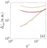
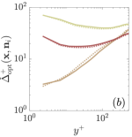
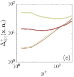
Figure 15: Comparison of the target resolutions corresponding to grids (a) DSM-3, (b) DSM-4 and (c) DSM-5 of Table 1 between error indicators computed using the original definition of Eqn. 6 (dotted lines) and the modified definition of Eqn. 28 (solid lines). The streamwise, wall-normal and spanwise resolutions are shown by the lightest to the darkest colors (in that order).

A better test-filter for this work would be one that more closely resembles the effect of implicit filtering (or cut-off) of the grid. For such filters the commutation errors can become larger, and thus more important.

Appendix D Comparison with the heuristic-based error indicator

In our previous work [13] we defined a heuristic-based error indicator as

$$\overline{\mathcal{A}}({\bf x},{\bf n})=\sqrt{\left\langle\overline{u}_{i}^{*,({\bf n})}\overline{u}_{i}^{*,({\bf n})}\right\rangle}$$ (29)

where $\overline{u}_{i}^{*,({\bf n})}=\overline{u}_{i}-\widehat{\overline{u}}_{i}^{({\bf n})}$ is the directionally high-pass test-filtered LES velocity field (using the same filter of Eqn. 2). From a physical point of view, $\overline{\mathcal{A}}({\bf x},{\bf n})$ only measures the small scale content of the velocity fields in any direction ${\bf n}$; however, if we employ the classical intuitive argument that the small scale energy controls both the numerical and modeling errors in LES [11, 12], we can assume that the errors are proportional to $\overline{\mathcal{A}}({\bf x},{\bf n})$ and thus use it as an error indicator.

It is useful to compare the grids generated by the proposed error indicator of this study (Eqn. 7) with those of Eqn. 29. In that sense, the results of this section complement our assessments of $\overline{\mathcal{G}}({\bf x},{\bf n})$ in Sections 3.2 and 4.

The flow setups used in [13] are slightly different from those used here; thus, all grid sequences are repeated for the exact flow setups of this paper. Additionally, we use the same grid selection criteria of Eqns. 12 and 13 ($\overline{\mathcal{G}}({\bf x},{\bf n})$ replaced by $\overline{\mathcal{A}}({\bf x},{\bf n})$), which is different from the prior work. Figure 16 shows a comparison of the optimal aspect ratios predicted by each error indicator for the test cases of this work.

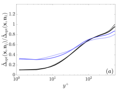
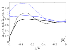
Figure 16: Examples of the predicted optimal cell aspect ratios $\check{\Delta}_{\rm opt}({\bf x},{\bf n}_{2})/\check{\Delta}_{\rm opt}({\bf x},{\bf n}_{1})$ (black lines) and $\check{\Delta}_{\rm opt}({\bf x},{\bf n}_{3})/\check{\Delta}_{\rm opt}({\bf x},{\bf n}_{1})$ (blue lines) using error indicators $\overline{\mathcal{A}}({\bf x},{\bf n})$ (solid lines) and $\overline{\mathcal{G}}({\bf x},{\bf n})$ (dotted lines) for (a) turbulent channel flow and (b) an $x$-normal plane inside the recirculation region ($x/H=2$) of the flow over a backward-facing step. Note that even in the channel flow where the predicted aspect ratios are similar, the difference in the spatial distribution of the two error indicators (combined with the structured nature of the grids) causes the final aspect ratios to be different from each other (since the minimum of streamwise and spanwise resolutions are reached at different $y$ locations).

The sequence of grids generated for LES of channel flow is summarized in Table 6. An interesting observation is the qualitative difference between the two sets of grids: although the grids generated using $\overline{\mathcal{A}}({\bf x},{\bf n})$ have a similar streamwise resolution to those generated by $\overline{\mathcal{G}}({\bf x},{\bf n})$, their wall-normal resolution is coarser near the wall and finer at the center of the channel (i.e., a flatter $\overline{\Delta}_{y}$ profile with a smaller stretching factor). This leads to a higher number of points across the channel that has to be compensated by a coarser spanwise resolution to keep $N_{\rm tot}$ constant.

Grid	$N_{\rm tot}$	$N_{y}$	$({\overline{\Delta}}_{x}^{+},\overline{\Delta}_{y_{w}}^{+}/2,{\overline{\Delta}}_{z}^{+})$	$({\overline{\Delta}}_{x},{\overline{\Delta}}_{y_{c}},{\overline{\Delta}}_{z})/H$	$Re_{\tau}$	$\overline{e}_{\rm QoI}^{\rm DNS}$ (%)
DSM-2	$74k$	34	$(77,5.6,55)$	$(0.14,0.099,0.10)$	553	11
A-2	$76k$	36	$(80,6.9,56)$	$(0.14,0.075,0.10)$	562	12
DSM-3	$251k$	44	$(53,2.3,29)$	$(0.098,0.091,0.054)$	536	7.3
A-3	$245k$	48	$(57,3.6,32)$	$(0.10,0.061,0.058)$	560	8.3
DSM-4	$514k$	50	$(45,1.7,19)$	$(0.082,0.080,0.035)$	544	3.3
A-4	$526k$	56	$(46,2.9,22)$	$(0.082,0.052,0.039)$	559	5.5
DSM-5	$1.18M$	60	$(34,1.4,13)$	$(0.063,0.065,0.024)$	544	1.8
A-5	$1.17M$	66	$(35,2.6,15)$	$(0.063,0.044,0.027)$	559	4.2
DSM-6	$2.53M$	72	$(25,1.6,10)$	$(0.046,0.052,0.018)$	542	1.1
A-6	$2.52M$	80	$(26,2.2,11)$	$(0.048,0.035,0.020)$	552	2.4
DSM-7	$5.80M$	90	$(18,1.4,7.6)$	$(0.033,0.041,0.014)$	540	1.1
A-7	$5.90M$	100	$(18,1.8,8.2)$	$(0.034,0.028,0.015)$	543	0.8
DSM-8	$11.1M$	108	$(14,1.2,6.3)$	$(0.025,0.033,0.012)$	541	0.9
A-8	$11.3M$	118	$(14,1.6,6.8)$	$(0.025,0.024,0.013)$	542	1.4

Table 6: Sequence of grids generated for LES of channel flow at $Re_{\tau}\approx 545$ using the dynamic Smagorinsky model. All A-$k$ grids are generated using the error indicator of Eqn. 29 and the criteria of Eqns. 12 and 13 with $\alpha=2$. Grids DSM-$k$ are simply copied from Table 1. See caption of Table 1 for more details.

Almost all grids generated using the new error indicator $\overline{\mathcal{G}}({\bf x},{\bf n})$ have lower values of the error metric $\overline{e}_{\rm QoI}^{\rm DNS}$. If we accept the lower values of $\overline{e}_{\rm QoI}^{\rm DNS}$ as a measure of optimality (this is not exactly true) we can conclude that the grids generated by $\overline{\mathcal{G}}({\bf x},{\bf n})$ have a more optimal distribution. This conclusion is consistent with our experience; in fact, grids generated by $\overline{\mathcal{A}}({\bf x},{\bf n})$ seem to have a slightly coarser resolution near the wall (especially in the last grids) compared to what we expect for such high-resolution grids.

Grid	$N_{\rm tot}$	$({\overline{\Delta}}_{x}^{+},\overline{\Delta}_{y_{w}}^{+}/2,{\overline{\Delta}}z^{+})$	$({\overline{\Delta}}_{x},{\overline{\Delta}}_{y},{\overline{\Delta}}_{z})/\delta_{\rm shear}$	$\overline{e}_{\rm QoI}^{\rm DNS}$ (%)
G-2	297k	$(42,2.6,21)$	$(0.16,0.078,0.16)$	10.5
A-2	297k	$(45,5.7,23)$	$(0.15,0.093,0.15)$	10.5
G-3	611k	$(45,1.4,11)$	$(0.16,0.049,0.078)$	5.6
A-3	599k	$(47,2.9,12)$	$(0.15,0.074,0.074)$	6.1
G-4	1.32M	$(47,1.5,12)$	$(0.076,0.038,0.076)$	4.9
A-4	1.35M	$(22,2.8,11)$	$(0.15,0.036,0.073)$	6.6
G-5	2.13M	$(25,0.77,6.2)$	$(0.070,0.035,0.035)$	5.4
A-5	2.17M	$(24,1.5,6.1)$	$(0.068,0.034,0.034)$	4.2
G-6	3.41M	$(25,0.77,6.1)$	$(0.068,0.034,0.034)$	3.5
A-6	3.70M	$(25,1.6,6.2)$	$(0.065,0.033,0.033)$	4.4
G-7	6.72M	$(12,0.76.6.0)$	$(0.034,0.017,0.034)$	2.5
A-7	7.26M	$(12,1.5,6.0)$	$(0.068,0.034,0.034)$	2.0

Table 7: Sequence of grids generated for LES of flow over a backward-facing step using $\overline{\mathcal{A}}({\bf x},{\bf n})$ of Eqn. 29 and grid selection criteria of Eqns. 12 and 13 with $\alpha=2$. Grids labeled by “G” are simply copied from Table 4. Refer to caption of Table 4 for more details including interpretation of each quantity.

As a second comparison we consider the flow over a backward-facing step, with results summarized in Table 7. The A-6 grid is shown in Fig. 17. Interestingly, we can identify the same general grid distribution patterns as what we saw in the channel flow; i.e., a general tendency to refine $\overline{\Delta}_{y}$ less near the wall and more towards the edge of the boundary layer, as well as refinement regions that are extended to a larger portion of the domain (for all three resolution directions).

Figure 17: Grid A-6 in Table 7 with 3.70M cells. Intersections of the blue planes highlight locations whose resolutions are reported in Table 7. Note that this grid is qualitatively different from G-6 shown in Fig. 13. See text for more details.

The error in (our specific) quantities of interest is generally lower for grids generated by $\overline{\mathcal{G}}({\bf x},{\bf n})$. Again, (assuming $\overline{e}_{\rm QoI}^{\rm DNS}$ as a measure of optimality) we can conclude that the grids generated by $\overline{\mathcal{G}}({\bf x},{\bf n})$ have a more optimal distribution. Once more, our experience with LES confirms this conclusion, as the reported resolutions in the boundary layer and shear layer of G-$k$ grids are closer to what we expect, especially in the last few grids with relatively high resolutions.

Appendix E Sensitivity to approximate implementations of the error indicator

In this section, we assess how sensitive the target grids are (in terms of error in QoIs and predicted distribution of filter-width) to approximations made when computing $\check{\mathcal{G}}({\bf x},{\bf n})$. This is of special interest to us because such approximations are almost unavoidable in practice, the most common of which happens when computing $\tau_{ij}^{\rm mod}(\widehat{\overline{u}}_{k}^{({\bf n})})$ in Eqn. 6. Examples of such approximations in the present study include: our assumption that the model coefficients remain unchanged between filter levels $\overline{\Delta}$ and $\widehat{\overline{\Delta}}^{({\bf n})}$ to avoid performing the full dynamic procedure (used in Sections 3.2 and 4), estimating the change in $\overline{k}_{\rm sgs}$ by an approximate formula to avoid solving an extra transport equation (Section 4), different numerics used in computing $\overline{\mathcal{G}}({\bf x},{\bf n})$ to avoid reimplementation of the exhaustively elaborate numerical schemes used in the LES solver, and so on.

As a relatively extreme test we use different LES models in the code and in computation of the error indicator. To this end, we generate five new sequences of grids, all starting from a grid with resolution of $(\overline{\Delta}_{x},\overline{\Delta}_{y},\overline{\Delta}_{z})/H=(0.20,0.10,0.20)$. In three of these sequences the constant Vreman model is used in the LES solver with $c_{v}=0.07$ and $\overline{\Delta}/\overline{h}=1$ (slightly different setup from what was used in Section 3.3 to test it in a regime of comparable magnitude for modeling and numerical errors), while $\tau_{ij}^{\rm mod}(\widehat{\overline{u}}_{k}^{({\bf n})})$ in the error indicator is computed once by the Vreman model (as it should), once by using the (dynamic) Smagorinsky model (Eqn. 17 of the paper), and once by setting the SGS terms to zero (${\tau}_{ij}^{\rm mod}\equiv 0$, corresponding to the DNS case). These three sets of grids are labeled “Vr$/$Vr”, “Vr$/$DSM” and “Vr$/$DNS”, respectively. Similarly, the other three sequences are generated by using the dynamic Smagorinsky model in the LES solver and using the Smagorinsky model in $\overline{\mathcal{G}}({\bf x},{\bf n})$ (labeled “DSM$/$DSM”), DSM in the solver and the Vreman model in the error indicator (labeled “DSM$/$Vr”) or setting the SGS terms to zero in the error indicator. The last sequence (corresponding to “DSM$/$DNS” grids) is discontinued after the fourth grid, since the target grids had identical resolutions (within two significant digits) to “DSM$/$Vr” grids.

The generated grids are summarized in Tables 8 (for sequences with the Vreman model in the LES solver) and 9 (for DSM). Convergence of $\overline{e}_{\rm QoI}^{\rm DNS}$ with total number of cells $N_{\rm tot}$ is further illustrated in Fig. 18.

Grid	$N_{\rm tot}$	$N_{y}$	$({\overline{\Delta}}_{x}^{+},\overline{\Delta}_{y_{w}}^{+}/2,{\overline{\Delta}}_{z}^{+})$	$({\overline{\Delta}}_{x},{\overline{\Delta}}_{y_{c}},{\overline{\Delta}}_{z})/H$	$Re_{\tau}$	$\overline{e}_{\rm QoI}^{\rm DNS}$ (%)
Vr$/$Vr-2	$74k$	34	$(70,4.0,47)$	$(0.14,0.10,0.097)$	488	19
Vr$/$DSM-2	$76k$	32	$(64,7.0,55)$	$(0.12,0.11,0.10)$	528	13
Vr$/$DNS-2	$76k$	36	$(70,3.3,46)$	$(0.15,0.096,0.097)$	476	20
Vr$/$Vr-3	$253k$	48	$(58,1.9,25)$	$(0.11,0.081,0.050)$	507	11
Vr$/$DSM-3	$246k$	40	$(41,3.8,33)$	$(0.078,0.10,0.063)$	526	11
Vr$/$DNS-3	$245k$	48	$(59,1.5,25)$	$(0.12,0.085,0.050)$	504	11
Vr$/$Vr-4	$513k$	52	$(46,2.0,18)$	$(0.089,0.076,0.034)$	516	8.1
Vr$/$DSM-4	$517k$	48	$(34,2.5,22)$	$(0.065,0.083,0.043)$	522	8.2
Vr$/$DNS-4	$512k$	54	$(46,1.1,18)$	$(0.091,0.075,0.035)$	511	8.4
Vr$/$Vr-5	$1.18M$	64	$(34,1.6,13)$	$(0.065,0.059,0.025)$	521	5.7
Vr$/$DSM-5	$1.17M$	60	$(29,2.0,15)$	$(0.054,0.065,0.028)$	525	5.8
Vr$/$DNS-5	$1.15M$	64	$(34,0.80,13)$	$(0.067,0.063,0.025)$	517	6.7
Vr$/$Vr-6	$2.54M$	76	$(25,1.4,10)$	$(0.047,0.049,0.019)$	527	4.2
Vr$/$DSM-6	$2.52M$	74	$(23,1.7,11)$	$(0.044,0.051,0.020)$	530	4.1
Vr$/$DNS-6	$2.50M$	78	$(25,0.61,10)$	$(0.048,0.050,0.020$	521	5.0
Vr$/$Vr-7	$5.85M$	96	$(18,1.1,7.8)$	$(0.033,0.037,0.019)$	531	3.6
Vr$/$DSM-7	$5.83M$	94	$(17,1.4,8.0)$	$(0.032,0.039,0.015)$	534	3.7
Vr$/$DNS-7	$5.80M$	98	$(18,0.47,7.9)$	$(0.034,0.038,0.015)$	527	3.7
Vr$/$Vr-8	$10.7M$	112	$(14,0.97,6.5)$	$(0.026,0.031,0.012)$	533	2.7
Vr$/$DSM-8	$10.8M$	110	$(14,1.2,6.5)$	$(0.025,0.032,0.012)$	535	2.8
Vr$/$DNS-8	$10.9M$	114	$(14,0.38,6.5)$	$(0.026,0.032,0.012)$	530	2.9

Table 8: Sensitivity of target grids to approximations in computation of $\tau_{ij}^{\rm mod}(\widehat{\overline{u}}_{k}^{({\bf n})})$ in Eqn. 6. All simulations use the constant Vreman model in the solver with $c_{v}=0.07$ and $\overline{\Delta}/\overline{h}=1$. Refer to caption of Table 1 for more details and interpretation of what each quantity means. See text for how grids “Vr$/$Vr”, “Vr$/$DSM” and “Vr$/$DNS” are generated.

Grid	$N_{\rm tot}$	$N_{y}$	$({\overline{\Delta}}_{x}^{+},\overline{\Delta}_{y_{w}}^{+}/2,{\overline{\Delta}}_{z}^{+})$	$({\overline{\Delta}}_{x},{\overline{\Delta}}_{y_{c}},{\overline{\Delta}}_{z})/H$	$Re_{\tau}$	$\overline{e}_{\rm QoI}^{\rm DNS}$ (%)
DSM$/$DSM-2	$74k$	34	$(77,5.6,55)$	$(0.14,0.099,0.10)$	553	11
DSM$/$Vr-2	$72k$	34	$(78,4.1,51)$	$(0.15,0.10,0.097)$	529	13
DSM$/$DSM-3	$251k$	44	$(53,2.3,29)$	$(0.098,0.091,0.054)$	536	7.3
DSM$/$Vr-3	$252k$	46	$(55,1.4,28)$	$(0.10,0.091,0.053)$	527	7.2
DSM$/$DSM-4	$514k$	50	$(45,1.7,19)$	$(0.082,0.080,0.035)$	544	3.3
DSM$/$Vr-4	$519k$	52	$(46,1.0,19)$	$(0.086,0.079,0.035)$	538	3.9
DSM$/$DSM-5	$1.18M$	60	$(34,1.4,13)$	$(0.063,0.065,0.024)$	544	1.8
DSM$/$Vr-5	$1.19M$	62	$(34,0.79,13)$	$(0.064,0.065,0.024)$	537	1.8
DSM$/$DSM-6	$2.53M$	72	$(25,1.6,10)$	$(0.046,0.052,0.018)$	542	1.1
DSM$/$Vr-6	$2.54M$	76	$(25,0.62,10)$	$(0.048,0.051,0.019)$	535	1.3
DSM$/$DSM-7	$5.80M$	90	$(18,1.4,7.6)$	$(0.033,0.041,0.014)$	540	1.1
DSM$/$Vr-7	$5.83M$	94	$(18,0.51,7.7)$	$(0.034,0.040,0.014)$	535	1.2
DSM$/$DSM-8	$11.1M$	108	$(14,1.2,6.3)$	$(0.025,0.033,0.012)$	541	0.9
DSM$/$Vr-8	$11.1M$	112	$(14,0.43,6.4)$	$(0.025,0.032,0.012)$	537	1.2

Table 9: Sensitivity of target grids to approximations in computation of $\tau_{ij}^{\rm mod}(\widehat{\overline{u}}_{k}^{({\bf n})})$ in Eqn. 6. Refer to caption of Table 1 for more details. All results are for LES using the dynamic Smagorinsky model. Grids labeled “DSM$/$DSM” are the same as those reported in Table 1 and are simply copied from there. See text for grids “DSM$/$Vr”.

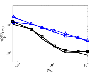
Figure 18: Sensitivity of error in the QoIs to approximations in computation of $\overline{\mathcal{G}}({\bf x},{\bf n})$. Figure summarizes results of Tables 8 and 9 for convergence of grids labeled as “DSM$/$DSM” (plain black line), “DSM$/$Vr” (black with squares), “Vr$/$Vr” (plain blue), “Vr$/$DSM” (blue with squares) and “Vr$/$DNS” (blue with triangles). See text and Tables for more details.

Note that (see Fig. 18) the error in the QoIs is not significantly affected by these relatively extreme inconsistencies in our implementation of the error indicator. The change in the target resolution is slightly more noticeable (Tables 8 and 9). For instance, the grid Vr$/$DSM-4 has a friction resolution of $(34,2.5,22)$ which is somewhat different from grid Vr-4 with resolution of $(46,2.0,18)$. Interestingly, this change in the target resolutions has a general trend that is present for almost all grids in the sequence (e.g., “DSM$/$Vr” grids have similar streamwise and spanwise resolutions compared to “DSM$/$DSM” grids, while their wall-normal resolution is finer adjacent to the wall). However, we should emphasize that despite the relative change in the resolution of the target grids these are still suitable grids for LES of wall bounded turbulence. In other words, the aspect ratio of the cells may be slightly affected and suboptimal, but the spanwise resolutions of the cells are still significantly finer than their streamwise resolution, and their wall-normal resolution is such that it resolves all the scales in the $y$ direction. The small change in $\overline{e}_{\rm QoI}^{\rm DNS}$ is in fact another proof of suitability of generated grids for channel flow: although this little effect on error in the QoIs is more related to the ability of the solver and its LES model in handling different grids, we can still conclude that the change in the target resolution is within some acceptable value to not deteriorate LES results significantly.

The presented results are specific to the LES code (numerics and models) and implementation of the error indicator used in this study, while the conclusion that the target grids are still close to what we would get by accurate implementation of the LES model is probably more general.

Appendix F Sensitivity of the target grids to the initial grid

In Sections 3 and 4 we tested the robustness of the error indicator and its target grids to coarse initial grids and underresolved turbulence. While in all cases the proposed methodology led to adapted grids that were quite close to what is considered “best-practice”, there are still two questions that remain to be answered: (i) how repeatable the generated grids are (i.e., if we can generate the same target grids by starting from a different initial grid), and (ii) how sensitive the final results are to the skeletal grid (i.e., if the proposed method can sufficiently refine the grid in all important regions, even if the maximum resolution is not limited by the skeletal grid). The goal of this section is to answer these two questions.

Only the flow over a backward-facing step is studied in this section. The sequence is started from an initial grid G-1^′ with a resolution of $({\overline{\Delta}}_{x},{\overline{\Delta}}_{y},{\overline{\Delta}}_{z})/H=(0.8,0.1,0.1)$. The reason for the finer spanwise resolution is to keep the flow turbulent. The skeletal grid in this section has a resolution of $(\Delta_{0,x},\Delta_{0,y},\Delta_{0,z})/H=(0.8,0.2,0.2)$ beyond which coarsening is not possible. At each iteration of the process $N_{\rm tot}$ is matched between grids G-$k^{\prime}$ of this section and G-$k$ (the original sequence in Section 4). The sequence is terminated once the next target grid is deemed sufficiently similar to its equivalent in the original sequence. The results are summarized in Table 10.

Grid	$N_{\rm tot}$	$(\overline{\Delta}_{x}^{+},\overline{\Delta}_{y_{w}}^{+}/2,\overline{\Delta}_{z}^{+})$	$(\overline{\Delta}_{x},\overline{\Delta}_{y},\overline{\Delta}_{z})/\delta_{\rm shear}$	$\overline{e}_{\rm QoI}^{\rm DNS}$ (%)
G-1′	79.6k	(173,11,22)	(1.2,0.14,0.14)	41
G-1	149k	$(42,10,42)$	$(0.21,0.17,0.33)$	11.1
G-2′	285k	(46,2.9,12)	(0.17,0.083,0.083)	15.5
G-2	297k	$(42,2.6,21)$	$(0.16,0.078,0.16)$	10.5
G-3′	570k	(45,1.4,11)	(0.15,0.038,0.076)	6.9
G-3	611k	$(45,1.4,11)$	$(0.16,0.049,0.078)$	5.6
G-4′	1.18M	(46,0.73,12)	(0.075,0.037,0.037)	5.2
G-4	1.32M	$(47,1.5,12)$	$(0.076,0.038,0.076)$	4.9

Table 10: Sequence of grids generated for LES of the flow over a backward-facing step starting from a different initial grid and how it compares with results of Section 4. See the caption of Table 4 for more details. Sequence is terminated at grid G-4^′ since from this point forward the target grids become nearly identical. Note that grid G-5^′ in Fig. 19 is generated from grid G-4^′, without the need for running the LES on it.

The difference between grids the G-$k^{\prime}$ and G-$k$ is quantified by the error in the refinement regions, $\overline{\mathcal{E}}_{\mathcal{R}}$, defined in Eqn. 19. In this section, $\overline{\mathcal{R}}_{\rm ref}$ is taken from grid G-$k$ and the integration domain is limited to $\Omega:{\bf x}=(x,y)\in[-20H,25H]\times[-H,0.5H]$ to eliminate the effect of coarser streamwise resolution of grids G-$k^{\prime}$ further away from the wall. The convergence of $\overline{\mathcal{E}}_{\mathcal{R}}$ with iteration number is shown in Fig. 19.

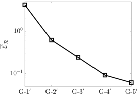
Figure 19: Decrease in the difference between grids G-$k^{\prime}$ and G-$k$ as the sequence progresses. The difference is characterized by $\overline{\mathcal{E}}_{\mathcal{R}}$ defined in Eqn. 19 with some modifications (see text for more details). Depending on the acceptable value of $\overline{\mathcal{E}}_{\mathcal{R}}$ either of grids G-4^′ ($\overline{\mathcal{E}}_{\mathcal{R}}\approx 0.09$) or G-5^′ ($\overline{\mathcal{E}}_{\mathcal{R}}\approx 0.06$) can be considered sufficiently close to grids G-4 and G-5 of Table 10.

Grid G-2^′ from Table 10 is illustrated by its refinement regions in Fig. 20. Note how different this first adapted grid is compared to grid G-2 illustrated in Fig. 8. Namely, the extremely coarse streamwise resolution of G-1^′ does not allow the solution, and thus the error indicator, to capture the recirculation bubble after the step and to resolve it on G-2^′. On the other hand, the coarser resolution of the skeletal grid gives the algorithm more flexibility to optimally distribute the filter-width, such that even on this coarse grid the wall-normal and spanwise resolutions are quite reasonable (both resolutions are finer than grid G-2).

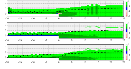
Figure 20: The grid G-2^′ from Table 10 illustrated by its refinement levels in $x$ (top), $y$ (middle), and $z$ (bottom). Refinement levels are computed based on a skeletal grid with $(\Delta_{0,x},\Delta_{0,y},\Delta_{0,z})/H=(0.8,0.2,0.2)$ for all ${\bf x}$ and ${\bf n}$. The light green, dark green and blue colors illustrate regions with one ($\overline{\Delta}_{{\bf n}_{x}}/H=0.4$ or $\overline{\Delta}_{{\bf n}_{y/z}}/H=0.1$), two ($\overline{\Delta}_{{\bf n}_{x}}/H=0.2$ or $\overline{\Delta}_{{\bf n}_{y/z}}/H=0.05$), and three ($\overline{\Delta}_{{\bf n}_{x}}/H=0.1$ or $\overline{\Delta}_{{\bf n}_{y/z}}/H=0.025$) refinement levels, respectively. The white regions correspond to areas of the domain that are left untouched (i.e., $\overline{\Delta}_{{\bf n}_{x}}/H=0.8$ or $\overline{\Delta}_{{\bf n}_{y/z}}/H=0.2$). The dashed line highlights the $\delta_{95}$ boundary layer thickness. Compare with Fig. 8.

Note that the results of this section are particular to this test case, and may not be necessarily true for other cases. For instance, if we had coarsened the grid enough such that it relaminarized, most probably the error indicator would have failed to predict the correct target grid. Besides, in transitional flows (including some separated flows where turbulence is triggered by the Kelvin-Helmholtz instability) the error indicator itself is probably not adequate and the adjoint fields may become necessary to capture the extreme sensitivity of the entire flowfield to those specific regions and to predict sufficient resolutions in those regions.

Appendix G More details on the test-filter and a more general class of suitable filters

The test-filter used throughout this work (Eqn. 2) is obtained by the van Cittert approximation to the implicit differential filter

$$\overline{\phi}=\left(I-\frac{\overline{\Delta}_{{\bf n}_{0}}^{2}}{4}{\bf n}_{0}^{T}\nabla\nabla^{T}{\bf n}_{0}\right)\widehat{\overline{\phi}}^{({\bf n}_{0})}\,,$$ (30)

which is a modified version of the filter originally proposed by Germano [34] to make it directionally dependent [see 13]. The van Cittert approximation is truncated after two terms to reduce the computational cost and complexity. Since this filter is used only to compute the error indicator, which is then only used to find the optimal filter-width, the effect of this truncation is assumed (and assessed) to be negligible in the final predictions of $\check{\Delta}_{\rm opt}({\bf x},{\bf n})$ (even though the computed values of the error indicator change). This is demonstrated in Fig. 21 for the example of LES of the channel flow using the dynamic Smagorinsky model.

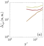
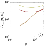
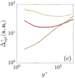
Figure 21: Comparison of the target resolutions corresponding to grids (a) DSM-2, (b) DSM-3 and (c) DSM-4 of Table 1 between error indicators computed using the approximate relation of Eqn. 2 (dotted lines) and the full deconvolution of Eqn. 30 (solid lines). The streamwise, wall-normal and spanwise resolutions are shown by the lightest to the darkest colors (in that order).

The current implementation of the filter (Eqn. 2) falls into a more general class of differential filters defined as [cf. 1, 32]

$$\widehat{\overline{\phi}}^{({\bf n}_{0})}=\sum_{k=0}^{\infty}{\frac{(-1)^{k}}{k!}{\overline{\Delta}}_{{\bf n}_{0}}^{k}M_{k}^{({\bf n}_{0})}\frac{\partial^{k}\overline{\phi}}{\partial x_{{\bf n}_{0}}^{k}}}$$ (31)

where $M_{k}^{({\bf n}_{0})}$ is the $k$th moment of the filter kernel (in direction ${\bf n}_{0}$). If only $k=0$ and $k\geq K$ are kept in the expansion [cf. 32], the commutation error of this general class of filters is of order $K$ (with some extra assumptions). In other words, by replacing the second derivative of Eqn. 2 with higher order derivates the commutation error of the filter and differentiation (which was assumed to be negligible in our derivations in Section 2.1) can be made sufficiently small. On structured grids with several neighbors available for each point higher derivatives are trivial to implement; however, in complex geometries (especially in the finite volume approach) computation of derivatives higher than $\partial^{2}/\partial x_{({\bf n}_{0})}^{2}$ are generally impractical (at least in the finite-volume framework). As a result, the filter used in this work was defined based on the second derivative with a commutation error of order $\Delta_{{\bf n}_{0}}^{2}$. The reason for the use of a differential filter is that it is easily applicable to complex geometries with fully unstructured grids, where the second derivative can be computed using the Taylor expansion and solving a least-square problem (see [64, 65, 13] for more details).

References

- [1] P. Sagaut, Large eddy simulation for incompressible flows, Springer Heidelberg, 2006.
- [2] S. Ghosal, An analysis of numerical errors in large-eddy simulations of turbulence, J. Comput. Phys. 125 (1996) 187–206.
- [3] N. Park, K. Mahesh, Analysis of numerical errors in large eddy simulation using statistical closure theory, J. Comput. Phys. 222 (2007) 194–216.
- [4] J. Gullbrand, F. K. Chow, The effect of numerical errors and turbulence models in large-eddy simulations of channel flow, with and without explicit filtering, J. Fluid Mech. 495 (2003) 323–341.
- [5] F. G. Kravchenko, P. Moin, On the effect of numerical errors in large eddy simulations of turbulent flows, J. Comput. Phys. 131 (1997) 310–322.
- [6] R. Mittal, P. Moin, Suitability of upwind-biased finite difference schemes for large-eddy simulation of turbulent flows, AIAA J. 35 (8) (1997) 1415–1417.
- [7] T. Brandt, A posteriori study on modelling and numerical error in LES applying the Smagorinsky model, in: Complex effects in large eddy simulations. Lecture notes in computational science and engineering, vol 56, Springer, Berlin, Heidelberg, 2007.
- [8] B. J. Geurts, J. Fröhlich, A framework for predicting accuracy limitations in large-eddy simulation, Phys. Fluids 14 (2002) L41.
- [9] I. B. Celik, Z. N. Cehreli, I. Yavuz, Index of resolution quality for large eddy simulations, J. Fluids Engr. 127 (2005) 939–958.
- [10] J. Jimenez, R. D. Moser, Large-eddy simulations: Where are we and what can we expect?, AIAA J. 38 (4) (2000) 605–612.
- [11] S. B. Pope, Ten questions concerning the large-eddy simulation of turbulent flows, New Journal of Physics 6 (2004) 35.
- [12] S. T. Bose, Explicitly filtered large-eddy simulation: with application to grid adaptation and wall modeling, PhD thesis, Stanford University (2012).
- [13] S. Toosi, J. Larsson, Anisotropic grid adaptation in large eddy simulations, Computers and Fluids 156 (2017) 146–161.
- [14] M. Klein, An attempt to assess the quality of large eddy simulations in the context of implicit filtering, Flow Turb. Comb. 75 (2005) 131–147.
- [15] M. Freitag, M. Klein, An improved method to assess the quality of large eddy simulations in the context of implicit filtering, J. Turbul. 7 (2006) N40.
- [16] M. Klein, J. Meyers, B. J. Geurts, Assessment of LES quality measures using the error landscape approach, in: Quality and reliability of large-eddy simulations. ERCOFTAC series, vol 12, Springer, Dordrecht, 2008.
- [17] I. Celik, M. Klein, M. Freitag, J. Janicka, Assessment measures for URANS/DES/LES: an overview with applications, J. Turbul. 7 (2009) 1–27.
- [18] I. Celik, M. Klein, J. Janicka, Assessment measures for engineering LES applications, J. Fluids Engr. 131 (2009) 031102–1.
- [19] P. Benard, G. Balarac, V. Moureau, C. Dobrzynski, G. Lartigue, Y. D’Angelo, Mesh adaptation for large-eddy simulations in complex geometries, Int. J. Num. Meth. Fluids 81 (2016) 719–740.
- [20] M. Klein, G. Scovazzi, M. Germano, On the Richardson extrapolation of the Reynolds stress with the Systematic Grid and Model Variation method, in: Direct and Large-Eddy Simulation XI. ERCOFTAC series, vol 25, Springer, Cham, 2019.
- [21] N. Legrand, G. Lartigue, V. Moureau, Adaptive multi-resolution large eddy simulation with control of modeling and numerical errors, in: 56th AIAA Aerospace Sciences Meeting, 2018.
- [22] J. Hoffman, C. Johnsson, Adaptive DNS/LES: a new agenda in CFD, Preprint, Chalmers Finite Element Center (2003).
- [23] J. Hoffman, On duality-based a posteriori error estimation in various norms and linear functionals for large eddy simulation, SIAM J. Sci. Comput. 26 (1) (2014) 178–191.
- [24] T. Barth, Space-time error representation and estimation in Navier-Stokes calculations, in: Complex effects in large eddy simulations. Lecture notes in computational science and engineering, vol 56, Springer, Berlin, Heidelberg, 2007.
- [25] Q. Wang, Forward and adjoint sensitivity computation of chaotic dynamical systems, J. Comput. Phys. 235 (2013) 1–13.
- [26] Q. Wang, Convergence of the least squares shadowing method for computing derivative of ergodic averages, SIAM J. Num. Anal. 52 (1) (2014) 156–170.
- [27] Y. Addad, U. Gaitonde, D. Laurence, S. Rolfo, Optimal unstructured meshing for large eddy simulations, in: Quality and reliability of large-eddy simulations. ERCOFTAC series, vol 12, Springer, Dordrecht, 2008.
- [28] A. Belme, A. Dervieux, F. Alauzet, Time accurate anisotropic goal-oriented mesh adaptation in unsteady flows, J. Comput. Phys. 231 (2012) 6323–6348.
- [29] M. Germano, U. Piomelli, P. Moin, W. H. Cabot, A dynamic subgrid-scale eddy viscosity model, Phys. Fluids 3 (7) (1991) 1760–1765.
- [30] D. K. Lilly, A proposed modification of the Germano subgrid-scale closure method, Phys. Fluids 4 (3) (1992) 633–635.
- [31] S. B. Pope, Turbulent Flows, Cambridge University Press, 2000.
- [32] O. V. Vasilyev, T. S. Lund, P. Moin, A general class of commutative filters for LES in complex geometries, J. Comput. Phys. 146 (1998) 82–104.
- [33] M. Germano, Differential filters of elliptic type, Phys. Fluids 29 (1986) 1757.
- [34] M. Germano, Differential filters for large eddy numerical simulation of turbulent flows, Phys. Fluids 29 (1986) 1755.
- [35] W. G. Habashi, J. Dompierre, Y. Bourgault, D. Ait-Ali-Yahya, M. Fortin, M. Vallet, Anisotropic mesh adaptation: towards user-independent, mesh-independent and solver-independent CFD. Part I: general principles, Int. J. Num. Meth. Fluids 32 (2000) 725–744.
- [36] J. Dompierre, M. Vallet, Y. Bourgault, M. Fortin, W. G. Habashi, Anisotropic mesh adaptation: towards user-independent, mesh-independent and solver-independent CFD. Part III. Unstructured meshes, Int. J. Num. Meth. Fluids 39 (2002) 675–702.
- [37] B. Vreman, B. Geurts, H. Kuerten, Large-eddy simulation of the temporal mixing layer using the Clark model, Theor. Comp. Fluid Dyn. 8 (1996) 309–324.
- [38] F. X. Trias, A. Gorobets, M. H. Silvis, R. W. C. P. Verstappen, A. Oliva, A new subgrid characteristic length for turbulence simulations on anisotropic grids, Phys. Fluids 29 (2017) 115109.
- [39] C. Meneveau, J. Katz, Scale-invariance and turbulence models for large-eddy simulation, Annu. Rev. Fluid Mech. 32 (2000) 1–32.
- [40] N. Park, K. Mahesh, Reduction of the Germano-identity error in the dynamic Smagorinsky model, Phys. Fluids 21 (2009) 065106.
- [41] Y. Morinishi, O. V. Vasilyev, A recommended modification to the dynamic two-parameter mixed subgrid scale model for large eddy simulation of wall bounded turbulent flow, Phys. Fluids 13 (11) (2001) 3400–3410.
- [42] M. Klein, M. Freitag, J. Janicka, Numerical determination of the scaling exponent of the modeled subgrid stresses for eddy viscosity models, in: Complex effects in large eddy simulations. Lecture notes in computational science and engineering, vol 56, Springer, Berlin, Heidelberg, 2007.
- [43] NRC, Assessing the reliability of complex models: Mathematical and statistical foundations of verification, validation, and uncertainty quantification, Tech. rep., National Research Council (2012).
- [44] K. J. Fidkowski, D. L. Darmofal, Review of output-based error estimation and mesh adaptation in computational fluid dynamics, AIAA J. 49 (4) (2011) 673–694.
- [45] D. J. Lea, M. R. Allen, T. W. N. Haine, Sensitivity analysis of the climate of a chaotic system, Tellus 52 (2000) 523–532.
- [46] J. Meyers, P. Sagaut, Is plane-channel flow a friendly case for the testing of large-eddy simulation subgrid-scale models?, Phys. Fluids 19 (2007) 048105.
- [47] S. Rezaeiravesh, M. Liefvendahl, Effect of grid resolution on large eddy simulation of wall-bounded turbulence, Phys. Fluids 30 (2018) 055106.
- [48] J. C. del Alamo, J. Jimenez, Spectra of the very large anisotropic scales in turbulent channels, Phys. Fluids 15 (6) (2003) L41–L43.
- [49] A. G. Kravchenko, P. Moin, R. Moser, Zonal embedded grids for numerical simulations of wall-bounded turbulent flows, J. Comput. Phys. 127 (1996) 412–423.
- [50] A. W. Vreman, An eddy-viscosity subgrid-scale model for turbulent shear flow: Algebraic theory and applications, Phys. Fluids 16 (10) (2004) 3670–3681.
- [51] S. Jovic, D. M. Driver, Backward-facing step measurements at low Reynolds number, , Tech. Mem. 108807, NASA (1994).
- [52] S. Jovic, D. M. Driver, Reynolds number effects on the skin friction in separated flows behind a backward facing step, Exp. Fluids 18 (1995) 464–467.
- [53] H. Le, P. Moin, J. Kim, Direct numerical simulation of turbulent flow over a backward-farcing step, J. Fluid Mech. 330 (1997) 349–374.
- [54] OpenFOAM Foundation, OpenFOAM description, http://www.openfoam.org (2019).
- [55] A. Yoshizawa, Bridging between eddy-viscosity-type and second-order models using a two-scale DIA, in: 9th Symposium on Turbulent Shear Flows, 1993.
- [56] W. Kim, S. Menon, A new dynamic one-equation subgrid-scale model for large eddy simulations, in: 33rd AIAA Aerospace Sciences Meeting, 1995.
- [57] S. Menon, W. W. Kim, High Reynolds number flow simulations using the localized dynamic subgrid-scale model, AIAA Paper 96 (1996) 0425.
- [58] X. Chai, K. Mahesh, Dynamic -equation model for large-eddy simulation of compressible flows, J. Fluid Mech. 699 (2012) 385–413.
- [59] D. C. Montgomery, G. C. Runger, Applied statistics and probability for engineers, ”Wiley & Sons”, 2011.
- [60] F. Porte-Agel, C. Meneveau, M. B. Parlange, A scale-dependent dynamic model for large-eddy simulation: application to a neutral atmospheric boundary layer, J. Fluid Mech. 415 (2000) 261–284.
- [61] S. T. Bose, P. Moin, D. You, Grid-independent large-eddy simulation using explicit filtering, Phys. Fluids 22 (2010) 105103.
- [62] E. Garnier, N. Adams, P. Sagaut, Large Eddy Simulation for Compressible Flows, Springer, 2009.
- [63] S. T. Bose, B. C. Wang, M. Saeedi, Prediction of unsteady heat transfer from a cylinder in crossflow, in: Proceedings of the Summer Program, Center for Turbulence Research, 2012, pp. 107–116.
- [64] P. J. Frey, F. Alauzet, Anisotropic mesh adaptation for CFD computations, Comput. Methods Appl. Mech. Engrg. 194 (2005) 5068–5082.
- [65] K. J. Fidkowski, D. L. Darmofal, A triangular cut-cell adaptive method for high-order discretizations of the compressible navier-stokes equations, J. Comput. Phys. 225 (2007) 1653–1672.