From computation to comparison of tensor decompositions

Abstract

Decompositions of higher-order tensors into sums of simple terms are ubiquitous. We show that in order to verify that two tensors are generated by the same (possibly scaled) terms it is not necessary to compute the individual decompositions. In general the explicit computation of such a decomposition may have high complexity and can be ill-conditioned. We now show that under some assumptions the verification can be reduced to a comparison of both the column and row spaces of the corresponding matrix representations of the tensors. We consider rank-1 terms as well as low multilinear rank terms (also known as block terms) and show that the number of the terms and their multilinear rank can be inferred as well. The comparison relies only on numerical linear algebra and can be done in a numerically reliable way. We also illustrate how our results can be applied to solve a multi-label classification problem that appears in the context of blind source separation.

15A23, 15A69

1 Introduction

Decompositions of tensors of order $N$ (i.e., $N$-way arrays of real or complex numbers) into a sum of simple terms are ubiquitous. The most common simple term is a rank-$1$ tensor, i.e. a nonzero tensor whose columns (resp. rows, fibers, etc.) are proportional. The corresponding decomposition into a minimal number of terms is known as Canonical Polyadic Decomposition (CPD).

It is well-known that for $N=2$, that is, in the matrix case, the decomposition in a minimal number of rank-$1$ terms is not unique unless the matrix itself is rank-$1$: indeed, any factorization $\mathbf{A}={\mathbf{X}}^{(1)}{\mathbf{X}}^{(2)T}$ with full column rank factors ${\mathbf{X}}^{(1)}=[\mathbf{x}^{(1)}_{1}\ \dots\ {\mathbf{x}}^{(1)}_{R}]$ and ${\mathbf{X}}^{(2)}=[\mathbf{x}^{(2)}_{1}\ \dots\ {\mathbf{x}}^{(2)}_{R}]$ generates a valid decomposition $\mathbf{A}=\mathbf{x}^{(1)}_{1}\mathbf{x}^{(2)T}_{1}+\dots+\mathbf{x}^{(1)}_{R}\mathbf{x}^{(2)T}_{R}$, where $R$ is the rank of $\mathbf{A}$, and this decomposition is not unique. On the other hand, if ${\mathbf{X}}^{(1)}$ and/or ${\mathbf{X}}^{(2)}$ are subject to constraints (e.g., triangularity or orthogonality), then the decomposition can be unique, but from an application point of view the imposed constraints can be unrealistic and the rank-$1$ terms not interpretable as meaningful “data components”. In contrast, for $N\geq 3$, that is, in the higher order tensor case, the unconstrained CPD is easily unique (see, for instance, [7, 8, 19, 20] and the references therein). Its uniqueness properties make the CPD a fundamental tool for unique retrieval of data components, latent variable analysis, independent component analysis, etc., with countless applications in chemometrics [6], telecommunication, array processing, machine learning, etc. [9, 10, 26, 27].

The higher order setting actually allows the recovery of terms that are more general than rank-$1$ terms. A MultiLinear (ML) rank-$(L_{1},L_{2},\dots)$ term is a tensor whose columns (resp. rows, fibers, etc.) form a matrix of rank $L_{1}$ (resp. $L_{2}$, $L_{3}$, etc.). Like CPD, a decomposition into a sum of ML rank-$(L_{1},L_{2},\dots)$ terms (also known as block term decomposition) is unique under reasonably mild assumptions (see [12, 21, 22] and the references therein), so that it has found applications in wireless communication [15], blind signal separation [13, 18], etc.

Tensor decompositions can be considered as tools for data analysis that allow one to break a single (tensor) data set into small interpretable components. It is known that, in general, the explicit computation of the CPD and the decomposition into a sum of ML rank-$(L_{1},L_{2},\dots)$ terms may have high complexity and can be ill-conditioned [1, 2, 5]. In other words, the mildness of the uniqueness conditions comes with a numerical and a computational cost.

In this paper we consider tensor decompositions from a fundamentally new perspective that is closer to pattern recognition. Namely, we consider the following “tensor similarity” problem:

• How to verify that two $I_{1}\times\dots\times I_{N}$ tensors are generated by the same (possibly scaled) rank-$1$ terms?

• More generally, how to verify that two $I_{1}\times\dots\times I_{N}$ tensors are generated by the same (possibly scaled) ML rank-$(L_{1},L_{2},\dots)$ terms?

For brevity, our presentation will be in terms of the more general variant. The simpler (C)PD variant will follow as a special case (see, for instance, Theorem 2.1).

An obvious approach would be to compute the decompositions of all tensors and then to compare them. This has two drawbacks. First, as mentioned above, the explicit computation of the decompositions may have high complexity and can be ill-conditioned. Second, the approach may fail if the tensors are generated by the same (possibly scaled) terms in cases where the decompositions are not unique.

In this paper we will not compute the tensor decompositions. We will pursue a different approach, starting from the following trivial observation: if

(1) $$\text{a tensor }\mathcal{B}\text{ is a sum of (possibly scaled) terms from the decomposition of a tensor }\mathcal{A},\\$$

then

(2) $$\operatorname{col}({\mathbf{B}}_{({S}^{c};S)})\subseteq\operatorname{col}({\mathbf{A}}_{({S}^{c};S)})\text{ for all proper subsets }S\text{ of }\{1,\dots,N\},$$

where $col(\cdot)$ denotes the column space of a matrix, $S^{c}$ denotes the complement of the set $S$, and ${\mathbf{A}}_{({S}^{c};S)}$ denotes the $(\prod\limits_{n\in S^{c}}I_{n})\times(\prod\limits_{n\in S}I_{n})$ matrix representation of $\mathcal{A}$ (see Section 4.2 for a formal definition of ${\mathbf{A}}_{({S}^{c};S)}$). Actually we will explain that Eq. 2 implies Eq. 1. A clear advantage of the approach based on the implication Eq. 2$\Rightarrow$Eq. 1 is that the conditions in Eq. 2 rely only on numerical linear algebra and can be verified in a numerically reliable way. On the other hand, it is not known whether Eq. 1 can always be replaced by Eq. 2.

Hence, the first contribution of this paper is to show that Eq. 2 implies Eq. 1. As a matter of fact, we will show that Eq. 1 follows from just $N$ conditions in Eq. 2, namely from the conditions

(3) $$\operatorname{col}({\mathbf{B}}_{({n}^{c};n)})\subseteq\operatorname{col}({\mathbf{A}}_{({n}^{c};n)}),\quad n\in\{1,\dots,N\},$$

and that the $\frac{I_{1}\cdots I_{N}}{I_{n}}\times I_{n}$ matrices ${\mathbf{A}}_{({n}^{c};n)}$ and ${\mathbf{B}}_{({n}^{c};n)}$ in Eq. 3 can be used to compute the number of terms in the decompositions of $\mathcal{A}$ and $\mathcal{B}$ as well as their multilinear ranks. We also consider a more general case where the inclusions in Eq. 3 are only known to hold for some $n$ in $\{1,\dots,N\}$.

It is worth noting that the conditions

(4) $$\operatorname{row}({\mathbf{B}}_{({n}^{c};n)})\subseteq\operatorname{row}({\mathbf{A}}_{({n}^{c};n)}),\quad n\in\{1,\dots,N\},$$

in which $row(\cdot)$ denotes the row space of a matrix, are more relaxed than the conditions in Eq. 3 (see Statement 1 of Lemma 3.2 below) and in general do not imply Eq. 1. For instance, if $\frac{I_{1}\cdots I_{N}}{I_{n}}\geq I_{n}$, then the conditions $\operatorname{row}({\mathbf{B}}_{({n}^{c};n)})=\operatorname{row}({\mathbf{A}}_{({n}^{c};n)})$ $(=\mathbb{F}^{I_{n}})$, $n\in\{1,\dots,N\}$ hold for any generic tensors $\mathcal{A}$ and $\mathcal{B}$ (no matter whether they are generated by the same (possibly scaled) terms or not).

The second contribution of this paper is to show that the remaining $2^{N}-2-N$ conditions in Eq. 2 are redundant, i.e., that the $N$ conditions in Eq. 3 imply all $2^{N}-2$ conditions in Eq. 2. (A fortiori, Eq. 1 follows from the $N$ conditions in Eq. 3, as mentioned under the “first contribution” above.)

Prior work on tensor similarity is limited to [31]. Both the present paper and [31] originated from the technical report [14]. The theoretical contributions of [31] related to the implication Eq. 3$\Rightarrow$ Eq. 1 rely on prior knowledge on the decompositions of $\mathcal{A}$ and $\mathcal{B}$ and can be summarized as follows: if $N=3$ and Eq. 3 holds with “$\subseteq$” replaced by “$=$”, then $\mathcal{A}$ and $\mathcal{B}$ are generated by the same (possibly scaled) terms. The results obtained in the current paper imply that the prior knowledge on the decompositions is not needed. Further, [31] presents applications in the context of emitter movement detection and fluorescence data analysis.

The paper is organized as follows. In Sections 2.1 and 2.2 we introduce tensor related notations and formalize the problem statement, respectively. Section 3 contains preliminary results. In Section 3.1, for the convenience of the reader, we remind the primary decomposition theorem and the Jordan canonical form. Section 3.2 contains an auxiliary result about the simultaneous compression of tensors $\mathcal{A}$ and $\mathcal{B}$ for which the first ${\hat{N}}$ inclusions in Eq. 3 hold (Lemma 3.2). The main results are given in Section 4. In Section 4.1 we establish connections between the terms in the decompositions of tensors $\mathcal{A}$ and $\mathcal{B}$ that satisfy the conditions in Eq. 3 (Theorems 4.1 and 4.3). In Section 4.2 we show that the $N$ conditions in Eq. 3 imply the $2^{N}-2$ conditions in Eq. 2 (Corollary 4.7). In Section 5 we illustrate how our results can be applied to solve a multi-label classification problem that appears in the context of blind source separation.

2 Basic definitions and problem statement

2.1 Basic definitions

Matrix representations

Let $1\leq n\leq N$. A mode-$n$ matrix representation of a tensor $\mathcal{A}\in\mathbb{F}^{I_{1}\times\dots\times I_{N}}$ is a matrix ${\mathbf{A}}_{({n}^{c};n)}\in\mathbb{F}^{\frac{I_{1}\cdots I_{N}}{I_{n}}\times I_{n}}$ whose columns are the vectorized mode-$n$ slices of $\mathcal{A}$. Using Matlab colon notation, the columns of ${\mathbf{A}}_{({n}^{c};n)}$ are the vectorized $I_{1}\times\dots\times I_{n-1}\times 1\times I_{n+1}\times\dots\times I_{N}$ tensors $\mathcal{A}(:,\dots,:,1,:,\dots,:),\dots,\mathcal{A}(:,\dots,:,I_{n},:,\dots,:)$. Formally,

(5) $$\text{the }(1+\sum_{\begin{subarray}{c}k=1\\ k\neq n\end{subarray}}^{N}(i_{k}-1)\prod_{\begin{subarray}{c}l=1\\ l\neq n\end{subarray}}^{k-1}I_{l},i_{n})\text{th entry of }{\mathbf{A}}_{({n}^{c};n)}=\text{ the }(i_{1},\dots,i_{N})\text{th entry of }\mathcal{A}.$$

Mode-$n$ product

If for some tensor $\mathcal{D}\in\mathbb{F}^{I_{1}\times\dots I_{n-1}\times L_{n}\times I_{n+1}\times I_{N}}$ and matrix $\mathbf{X}^{(n)}\in\mathbb{F}^{I_{n}\times L_{n}}$,

(6) $${\mathbf{A}}_{({n}^{c};n)}={\mathbf{D}}_{({n}^{c};n)}\mathbf{X}^{(n)T},$$

i.e., if the mode-$n$ fibers of $\mathcal{A}$ are obtained by multiplying the corresponding mode-$n$ fibers of $\mathcal{D}$ by $\mathbf{X}^{(n)}$, then we say that $\mathcal{A}$ is the mode-$n$ product of a $\mathcal{D}$ and $\mathbf{X}^{(n)}$ and write $\mathcal{A}=\mathcal{D}\bullet_{n}\mathbf{X}^{(n)}$. It can be easily verified that the remaining $N-1$ matrix representations of $\mathcal{A}$ can be factorized as

(7) $${\mathbf{A}}_{({k}^{c};k)}=\left(\bigotimes_{l=1,l\neq k}^{n-1}\mathbf{I}_{I_{l}}\otimes\mathbf{X}^{(n)}\otimes\bigotimes_{l=n+1,l\neq k}^{N}\mathbf{I}_{I_{l}}\right){\mathbf{D}}_{({k}^{c};k)},\qquad k\in\{1,\dots,N\}\setminus\{n\}.$$

where $\mathbf{I}_{I_{l}}$ and “$\otimes$” denote the $I_{l}\times I_{l}$ identity matrix and the Kronecker product, respectively.

Several products in the same mode or across modes

It easily follows from Eq. 6 that for compatible matrix and tensor dimensions,

$$\left(\left(\left(\mathcal{D}\bullet_{n}\mathbf{X}_{1}^{(n)}\right)\bullet_{n}\mathbf{X}_{2}^{(n)}\right)\dots\bullet_{n}\mathbf{X}_{k}^{(n)}\right)=\mathcal{D}\bullet_{n}\left(\mathbf{X}_{k}^{(n)}\cdots\mathbf{X}_{1}^{(n)}\right).$$

Let ${\hat{N}}\leq N$ and

(8) $$\mathcal{D}\in\mathbb{F}^{L_{1}\times\dots\times L_{{\hat{N}}}\times I_{{\hat{N}}+1}\times\dots\times I_{N}},\qquad\mathbf{X}^{(1)}\in\mathbb{F}^{I_{1}\times L_{1}},\dots,\mathbf{X}^{({\hat{N}})}\in\mathbb{F}^{I_{{\hat{N}}}\times L_{{\hat{N}}}}.$$

For products across different modes, we have

(9) $$\mathcal{D}\bullet_{1}\mathbf{X}^{(1)}\dots\bullet_{N}\mathbf{X}^{(N)}:= \left(\left(\left(\mathcal{D}\bullet_{1}\mathbf{X}^{(1)}\right)\bullet_{2}\mathbf{X}^{(2)}\right)\dots\bullet_{N}\mathbf{X}^{(N)}\right)=$$

$$\left(\left(\left(\mathcal{D}\bullet_{i_{1}}\mathbf{X}^{(i_{1})}\right)\bullet_{i_{2}}\mathbf{X}^{(i_{2})}\right)\dots\bullet_{i_{N}}\mathbf{X}^{(i_{N})}\right)$$

for any permutation $i_{1},\dots,i_{N}$ of $1,\dots,N$. It follows from Eqs. 6, 7 and 9, that the matrix representations of $\mathcal{A}=\mathcal{D}\bullet_{1}\mathbf{X}^{(1)}\dots\bullet_{N}\mathbf{X}^{(N)}$ are given by

(10) $${\mathbf{A}}_{({n}^{c};n)}=\left(\bigotimes_{k=1,k\neq n}^{N}\mathbf{X}^{(k)}\right){\mathbf{D}}_{({n}^{c};n)}\mathbf{X}^{(n)T},\qquad n\in\{1,\dots,N\}.$$

If $\mathcal{A}=\mathcal{D}\bullet_{1}\mathbf{X}^{(1)}\dots\bullet_{{\hat{N}}}\mathbf{X}^{({\hat{N}})}$ with ${\hat{N}}<N$, then the identities in Eq. 10 hold with $\mathbf{X}^{({\hat{N}}+1)}=\mathbf{I}_{I_{{\hat{N}}+1}},\dots,\mathbf{X}^{(N)}=\mathbf{I}_{I_{N}}$. That is,

(11) $${\mathbf{A}}_{({n}^{c};n)} =\left(\bigotimes_{k=1,k\neq n}^{{\hat{N}}}\mathbf{X}^{(k)}\otimes\bigotimes_{k={\hat{N}}+1}^{N}\mathbf{I}_{I_{k}}\right){\mathbf{D}}_{({n}^{c};n)}\mathbf{X}^{(n)T},\qquad n\in\{1,\dots,{\hat{N}}\},$$

(12) $${\mathbf{A}}_{({n}^{c};n)} =\left(\bigotimes_{k=1}^{{\hat{N}}}\mathbf{X}^{(k)}\otimes\bigotimes_{k={\hat{N}}+1,k\neq n}^{N}\mathbf{I}_{I_{k}}\right){\mathbf{D}}_{({n}^{c};n)},\qquad n\in\{{\hat{N}}+1,\dots,N\}.$$

ML rank of a tensor

By definition,

$$\mathcal{A}\ \text{ is ML rank-}(L_{1},\dots,L_{{\hat{N}}},\cdot,\dots,\cdot)\overset{\text{def}}{\Longleftrightarrow}r_{{\mathbf{A}}_{({n}^{c};n)}}=L_{n},\quad n\in\{1,\dots,{\hat{N}}\},\quad 2\leq{\hat{N}}\leq N,$$

that is, $L_{n}$ is the dimension of the subspace spanned by the mode-$n$ fibers of $\mathcal{A}$. It can be shown that $\mathcal{A}$ is ML rank-$(L_{1},\dots,L_{{\hat{N}}},\cdot,\dots,\cdot)$ if and only if it admits the factorization $\mathcal{A}=\mathcal{D}\bullet_{1}\mathbf{X}^{(1)}\dots\bullet_{{\hat{N}}}\mathbf{X}^{({\hat{N}})}$ such that $\mathcal{D}$, $\mathbf{X}^{(1)},\dots,\mathbf{X}^{({\hat{N}})}$ have dimensions as in Eq. 8 and $\mathbf{X}^{(1)},\dots,\mathbf{X}^{({\hat{N}})},{\mathbf{D}}_{({1}^{c};1)},\dots,{\mathbf{D}}_{({{\hat{N}}}^{c};{\hat{N}})}$ have full column rank. In this paper we assume that the tensor dimensions have been permuted so that we can just specify the rank values for the first ${\hat{N}}$ matrix representations of $\mathcal{A}$. A special case of the factorization $\mathcal{A}=\mathcal{D}\bullet_{1}\mathbf{X}^{(1)}\dots\bullet_{{\hat{N}}}\mathbf{X}^{({\hat{N}})}$, where ${\hat{N}}=N$, $\mathbf{X}^{(n)}$ equals the “$U$” factor in the compact Singular Values Decomposition (SVD) of ${\mathbf{A}}_{({n}^{c};n)}$, and $\mathcal{D}=\mathcal{A}\bullet_{1}\mathbf{X}^{(1)H}\dots\bullet_{N}\mathbf{X}^{(N)H}$ is known as the MLSVD of $\mathcal{A}$ and is used for the compression of an $I_{1}\times\dots\times I_{N}$ tensor to the size $L_{1}\times\dots\times L_{N}$ [16]. By setting $\mathbf{X}^{(n)}$ equal to the identity matrix for $n={\hat{N}}+1,\dots,N$, we compress only along the first ${\hat{N}}$ dimensions.

ML rank-$(L_{1r},\dots,L_{{\hat{N}}r},\cdot,\dots,\cdot)$ decomposition of a tensor

In this paper we consider the decomposition of $\mathcal{A}$ into a sum of ML rank-$(L_{1r},\dots,L_{{\hat{N}}r},\cdot,\dots,\cdot)$ terms:

(13) $$\mathcal{A}=\sum\limits_{r=1}^{R}\mathcal{D}_{r}\bullet_{1}\mathbf{X}^{(1)}_{r}\dots\bullet_{\hat{N}}\mathbf{X}^{({\hat{N}})}_{r},\quad 2\leq{\hat{N}}\leq N,$$

$$\mathcal{D}_{r}\in\mathbb{F}^{L_{1r}\times\dots\times L_{{\hat{N}}_{r}}\times I_{{\hat{N}}_{r}+1}\times\dots\times I_{N}},\quad\mathbf{X}^{(n)}_{r}\in\mathbb{F}^{I_{n}\times L_{nr}},\quad n\in\{1,\dots,{\hat{N}}\},\quad r\in\{1,\dots,R\}.$$

In our derivation we will also use a matricized version of Eq. 13. It can be obtained as follows. First, we call

(14) $$\mathbf{X}^{(n)}:=[\mathbf{X}^{(n)}_{1}\ \dots\ \mathbf{X}^{(n)}_{R}]\in\mathbb{F}^{I_{n}\times\sum\limits_{r=1}^{R}L_{nr}},\qquad n\in\{1,\dots,{\hat{N}}\},$$

the concatenated factor matrices of $\mathcal{A}$. If further we set

(15) $$\mathbf{X}^{(n)}:=[\mathbf{I}_{I_{n}}\ \dots\ \mathbf{I}_{I_{n}}]\in\mathbb{F}^{I_{n}\times RI_{n}},\qquad n\in\{{\hat{N}}+1,\dots,N\},$$

then, by Eq. 10, we can express Eq. 13 in a matricized way as

(16) $${\mathbf{A}}_{({n}^{c};n)}=\sum\limits_{r=1}^{R}\left(\bigotimes_{l=1,l\neq n}^{N}\mathbf{X}_{r}^{(l)}\right){{\mathbf{D}}_{r}}_{({n}^{c};n)}\mathbf{X}_{r}^{(n)T}=\\ \left(\bigodot\limits_{l=1,l\neq n}^{N}\mathbf{X}^{(l)}\right)\operatorname{Bdiag}({{\mathbf{D}}_{1}}_{({n}^{c};n)},\dots,{{\mathbf{D}}_{R}}_{({n}^{c};n)})\mathbf{X}^{(n)T},\qquad n\in\{1,\dots,N\},$$

where

(17) $$\bigodot\limits_{l=1,l\neq n}^{N}\mathbf{X}^{(l)}:=\left[\bigotimes_{l=1,l\neq n}^{N}\mathbf{X}_{1}^{(l)}\ \dots\ \bigotimes_{l=1,l\neq n}^{N}\mathbf{X}_{R}^{(l)}\right]$$

and $\operatorname{Bdiag}({{\mathbf{D}}_{1}}_{({n}^{c};n)},\dots,{{\mathbf{D}}_{R}}_{({n}^{c};n)})$ denotes a block-diagonal matrix with the matrices ${{\mathbf{D}}_{1}}_{({n}^{c};n)}$, $\dots$, ${{\mathbf{D}}_{R}}_{({n}^{c};n)}$ on the diagonal.

Note that Eq. 13 captures several well-studied decompositions as special cases (see also the introduction). If ${\hat{N}}=N$ and $L_{1r}=\dots=L_{Nr}=1$ for all $r$, then all terms in Eq. 13 are rank-$1$ tensors, so Eq. 13 reduces to a polyadic decomposition of $\mathcal{A}$. It can easily be verified that if ${\hat{N}}=2$, $N=3$, and $L_{1r}=1$ for all $r$, then the ML rank-$(1,L_{2r},\cdot)$ terms in Eq. 13 are actually ML rank-$(1,L_{2r},L_{2r})$ terms. Thus, Eq. 13 reduces to the decomposition into a sum of ML rank-$(1,L_{2r},L_{2r})$ terms. Finally, if ${\hat{N}}=2$ and $N=3$, then Eq. 13 is a tensor reformulation of the joint block diagonalization problem. Namely, Eq. 13 means that the frontal slices of $\mathcal{A}$ can simultaneously be factorized as

$$\mathbf{A}(:,:,i)=\mathbf{X}^{(1)}\operatorname{Bdiag}({\mathbf{D}}_{1}(:,:,i),\dots,{\mathbf{D}}_{R}(:,:,i))\mathbf{X}^{(2)T},\quad i=1,\dots,I_{3},$$

where ${\mathbf{D}}_{r}(:,:,i)\in\mathbb{F}^{L_{1r}\times L_{2r}}$.

2.2 Problem statement

Assume that a tensor $\mathcal{B}\in\mathbb{F}^{I_{1}\times\dots\times I_{N}}$ consists of the same ML rank-$(L_{1r},\dots,L_{{\hat{N}}r},\cdot,\dots,\cdot)$ terms as $\mathcal{A}$, but possibly differently scaled:

(18) $$\mathcal{B}=\sum\limits_{r=1}^{R}\lambda_{r}\mathcal{D}_{r}\bullet_{1}\mathbf{X}^{(1)}_{r}\dots\bullet_{\hat{N}}\mathbf{X}^{({\hat{N}})}_{r},\qquad\lambda_{1}\cdots\lambda_{R}\neq 0.$$

Then by Eq. 16,

(19) $${\mathbf{B}}_{({n}^{c};n)}=\left(\bigodot\limits_{k=1,k\neq n}^{N}\mathbf{X}^{(k)}\right)\operatorname{Bdiag}(\lambda_{1}{{\mathbf{D}}_{1}}_{({n}^{c};n)},\dots,\lambda_{R}{{\mathbf{D}}_{R}}_{({n}^{c};n)})\mathbf{X}^{(n)T}=\\ \left(\bigodot\limits_{k=1,k\neq n}^{N}\mathbf{X}^{(k)}\right)\operatorname{Bdiag}({{\mathbf{D}}_{1}}_{({n}^{c};n)},\dots,{{\mathbf{D}}_{R}}_{({n}^{c};n)})\operatorname{Bdiag}(\lambda_{1}\mathbf{I}_{L_{n1}},\dots,\lambda_{R}\mathbf{I}_{L_{nR}})\mathbf{X}^{(n)T}.$$

Assume that ${\hat{N}}\geq 2$ and that the matrices

(20) $$\mathbf{X}^{(1)},\dots,\mathbf{X}^{({\hat{N}})}\ \text{ have full column rank.}$$

It can be easily shown that the matrices in Eq. 17 have full column rank for all $n$. Hence, by Eqs. 16 and 19, the column spaces of the first ${\hat{N}}$ matrix representations of $\mathcal{A}$ and $\mathcal{B}$ coincide:

(21) $$\operatorname{col}({\mathbf{A}}_{({n}^{c};n)})=\operatorname{col}({\mathbf{B}}_{({n}^{c};n)}),\qquad n\in\{1,\dots,{\hat{N}}\}.$$

If we further limit ourselves to the case where the matrices

(22) $$\mathbf{X}^{(1)},\dots,\mathbf{X}^{({\hat{N}})}\ \text{ are square and nonsingular,}$$

then, obviously,

(23) $${\mathbf{B}}_{({n}^{c};n)}={\mathbf{A}}_{({n}^{c};n)}\mathbf{M}_{n},\qquad n\in\{1,\dots,{\hat{N}}\},$$

where

(24) $$\mathbf{M}_{n}=\left(\mathbf{X}^{(n)T}\right)^{-1}\operatorname{Bdiag}(\lambda_{1}\mathbf{I}_{L_{n1}},\dots,\lambda_{R}\mathbf{I}_{L_{nR}})\mathbf{X}^{(n)T},\qquad n\in\{1,\dots,{\hat{N}}\}.$$

Thus, if Eqs. 13, 18 and 22 hold, then the column spaces of the first ${\hat{N}}$ matrix representations of $\mathcal{A}$ and $\mathcal{B}$ coincide, the matrices $\mathbf{M}_{n}:={{\mathbf{A}}^{\dagger}_{(n^{c};n)}}{\mathbf{B}}_{({n}^{c};n)}$ have the same spectrum $\lambda_{1},\dots,\lambda_{R}\in\mathbb{F}$ and can be diagonalized, $n=1,\dots,{\hat{N}}$. Moreover, the concatenated factor matrices $\mathbf{X}^{(n)}$ and the sizes of blocks $L_{nr}$ (and hence the overall decompositions of $\mathcal{A}$ and $\mathcal{B}$) can be recovered from the EVDs of $\mathbf{M}_{1},\dots,\mathbf{M}_{\hat{N}}$.

In this paper we consider the inverse problem: we assume that the column spaces of the first ${\hat{N}}$ matrix representations of $\mathcal{A}$ and $\mathcal{B}$ coincide and we investigate how the ML rank decompositions $\mathcal{A}$ and $\mathcal{B}$ relate to each other. In particular, we obtain the following result.

Theorem 2.1.

Let $\mathcal{A},\mathcal{B}\in\mathbb{C}^{I_{1}\times\dots\times I_{N}}$ and $2\leq{\hat{N}}\leq N$. Assume that Eqs. 22 and 23 hold and that at least one of the matrices $\mathbf{M}_{1},\dots,\mathbf{M}_{{\hat{N}}}$ can be diagonalized. Then the following statements hold.

1. The matrices $\mathbf{M}_{1},\dots,\mathbf{M}_{{\hat{N}}}$ have the same spectrum.

2. All matrices $\mathbf{M}_{1},\dots,\mathbf{M}_{{\hat{N}}}$ can be diagonalized.

3. Let the distinct eigenvalues of $\mathbf{M}_{n}$ be $\lambda_{1},\dots,\lambda_{R}$ with respective multiplicities $L_{n1},\dots,L_{nR}$ and let $\mathbf{X}_{n}\in\mathbb{C}^{I_{n}\times I_{n}}$ be a nonsingular matrix such that Eq. 24 holds. Then $\mathcal{A}$ and $\mathcal{B}$ admit the ML rank-$(L_{1r},\dots,L_{{\hat{N}}r},\cdot,\dots,\cdot)$ decompositions in Eqs. 13 and 18, respectively. In particular, if $L_{nr}=1$ for all $n$ and $r$, then $\mathcal{A}$ and $\mathcal{B}$ are generated by the same (possibly scaled) $R$ rank-$1$ terms.

Proof 2.2.

The proof follows from Theorem 4.3 below.

The theorem can be used as follows. First, the matrices $\mathbf{M}_{1},\dots,\mathbf{M}_{{\hat{N}}}$ are found from the sets of linear equations Eq. 23. (If any of the sets of linear equations does not have a solution, then $\mathcal{B}$ is not of the form Eq. 18, i.e., it cannot be generated by terms from the decomposition of $\mathcal{A}$.) The number of terms $R$ is found as the number of distinct eigenvalues of $\mathbf{M}_{n}$, $1\leq n\leq{\hat{N}}$. The distinct eigenvalues themselves correspond to the scaling factors $\lambda_{r}$ in Eq. 18. Both $R$ and the eigenvalues $\lambda_{r}$ are necessarily the same for all $\mathbf{M}_{n}$, but the multiplicities can be different. The multiplicity of $\lambda_{r}$ in the EVD of $\mathbf{M}_{n}$ corresponds to the $n$th entry $L_{nr}$ in the ML rank of the $r$th term. The larger ${\hat{N}}$, the more the terms are specified. The minimal value for ${\hat{N}}$ is $2$, since a decomposition in ML rank-$(L_{1r},\cdot,\dots,\cdot)$ terms is meaningless.

So far, we have explained the use of the theorem for decompositions that are exact. Obviously, the theorem also suggests a procedure for approximate decompositions (of noisy tensors). The equations in Eq. 23 may be solved in least squares sense. The eigenvalues $\lambda_{nr}$ of the matrices $\mathbf{M}_{1},\dots,\mathbf{M}_{{\hat{N}}}$ may be averaged over $n$ to obtain estimates of $\lambda_{r}$. The values $L_{nr}$, $1\leq n\leq{\hat{N}}$, $1\leq r\leq R$ may be estimated by assessing how close the eigenvalues $\lambda_{rn}$ are to the averaged values $\lambda_{r}$.

3 Preliminaries

3.1 Primary decomposition theorem and the Jordan canonical form

In this subsection we recall known results that will be used in Section 4. Recall that the minimal polynomial $q(x)$ of a matrix $\mathbf{M}\in\mathbb{F}^{I\times I}$ is the polynomial of least degree over $\mathbb{F}$ whose leading coefficient is $1$ and such that $q(\mathbf{M})=\mathbf{O}$. It is well known that the minimal polynomial does not depend of $\mathbb{F}$, is unique, and that the set of its zeros coincides with the set of the eigenvalues of the matrix (in the case $\mathbb{F}=\mathbb{R}$ both sets can be empty, namely, when the minimal polynomial does not have real roots). Recall also that a non-constant polynomial is irreducible over $\mathbb{F}$ if its coefficients belong to $\mathbb{F}$ and it cannot be factorized into the product of two non-constant polynomials with coefficients in $\mathbb{F}$. For instance, the minimal polynomials of the matrices

$$\begin{bmatrix}0&0\\ 1&1\end{bmatrix},\quad\begin{bmatrix}0&1\\ 1&0\end{bmatrix},\quad\begin{bmatrix}0&1\\ -1&0\end{bmatrix},\quad\begin{bmatrix}0&1\\ 0&0\end{bmatrix},\text{ and }\mathbf{I}_{I}$$

are $x^{2}-x$, $x^{2}-1$, $x^{2}+1$, $x^{2}$, and $x-1$, respectively. The matrix $\mathbf{I}_{I}$ has a single eigenvalue $1$ of multiplicity $I$ which corresponds to a single root of $x-1$ of multiplicity $1$. The polynomial $x^{2}+1$ is irreducible over $\mathbb{R}$ and is reducible over $\mathbb{C}$, $x^{2}+1=(x+i)(x-i)$, which agrees with the fact that the matrix $\begin{bmatrix}0&1\\ -1&0\end{bmatrix}$ does not have eigenvalues over $\mathbb{R}$ but has two eigenvalues $-i$ and $i$ over $\mathbb{C}$. It is well known that any polynomial with leading coefficient $1$ can be factorized as

$$q(x)=p_{1}(x)^{\mu_{1}}\cdots p_{R}(x)^{\mu_{R}}$$

where $p_{r}$ are distinct irreducible polynomials and $\mu_{r}\geq 1$. Since in this paper $\mathbb{F}$ is either $\mathbb{C}$ or $\mathbb{R}$, we have that

$$p_{1},\dots,p_{R}\in\{x-\lambda:\ \lambda\in\mathbb{C}\},\text{ if }\mathbb{F}=\mathbb{C},$$

$$p_{1},\dots,p_{R}\in\{x-\lambda:\ \lambda\in\mathbb{R}\}\cup\{x^{2}+2ax+a^{2}+b^{2}:\ a,b\in\mathbb{R}\text{ and }b>0\},\text{ if }\ \mathbb{F}=\mathbb{R}.$$

The following theorem implies that the minimal polynomial of a matrix can be used to construct a basis in which that matrix has block-diagonal form.

Theorem 3.1 (Primary decomposition theorem [11, pp.196–197]).

Let $\mathbf{M}\in\mathbb{F}^{I\times I}$ and let

$$q(x)=p_{1}(x)^{\mu_{1}}\cdots p_{R}(x)^{\mu_{R}}$$

be the minimal polynomial of $\mathbf{M}$, factorized into powers of distinct polynomials $p_{r}(x)$ that are irreducible (over $\mathbb{F}$). Then the subspaces

$$E_{r}:=\operatorname{Null}\left(p_{r}(\mathbf{M})^{\mu_{r}}\right),\quad 1\leq r\leq R$$

are invariant for $\mathbf{M}$, i.e., $\mathbf{M}E_{r}\subseteq E_{r}$ and we have

(25) $$\mathbb{F}^{I}=E_{1}\oplus\cdots\oplus E_{R},$$

where “$\oplus$” denotes the direct sum of subspaces.

Decomposition Eq. 25 in Theorem 3.1 implies that the matrix $\mathbf{M}$ is similar to a block-diagonal matrix. Indeed, let $L_{r}=\dim E_{r}$ and let the columns of $\mathbf{S}_{r}\in\mathbb{F}^{I\times L_{r}}$ form a basis of $E_{r}$, $r=1,\dots,R$. Then by Eq. 25, the columns of $\mathbf{S}:=[\mathbf{S}_{1}\ \dots\ \mathbf{S}_{R}]$ form a basis of the entire space $\mathbb{F}^{I}$, implying that $\mathbf{S}$ is nonsingular. Since $\mathbf{M}E_{r}\subseteq E_{r}$ it follows that there exists a unique matrix $\mathbf{T}_{r}\in\mathbb{F}^{L_{r}\times L_{r}}$ such that $\mathbf{M}\mathbf{S}_{r}=\mathbf{S}_{r}\mathbf{T}_{r}$, $r=1,\dots,R$. Hence $\mathbf{M}[\mathbf{S}_{1}\ \dots\ \mathbf{S}_{R}]=[\mathbf{S}_{1}\mathbf{T}_{1}\ \dots\ \mathbf{S}_{R}\mathbf{T}_{R}]$ or

$$\mathbf{M}=\mathbf{S}\operatorname{Bdiag}(\mathbf{T}_{1},\dots,\mathbf{T}_{R})\mathbf{S}^{-1},\quad\mathbf{S}=[\mathbf{S}_{1}\ \dots\ \mathbf{S}_{R}],\quad\mathbf{S}_{r}\in\mathbb{F}^{I\times L_{r}}.$$

It is well-known that each of the matrices $\mathbf{T}_{r}$ can further be reduced to Jordan canonical form by a similarity transform. Namely, if $p_{r}(x)^{\mu_{r}}=(x-\lambda)^{\mu_{r}}$ with $\lambda\in\mathbb{F}$, then $\mathbf{T}_{r}$ is similar to $J(\lambda,n_{r1})\oplus\dots\oplus J(\lambda,n_{rk_{r}})$, where $J(\lambda,n)$ denotes the $n\times n$ Jordan block with $\lambda$ on the main diagonal:

$$\begin{bmatrix}\lambda&1&0&\dots&0\\ 0&\lambda&1&\dots&0\\ \vdots&\vdots&\vdots&\vdots&\vdots\\ 0&0&0&\dots&1\\ 0&0&0&\dots&\lambda\end{bmatrix}.$$

If $\mathbb{F}=\mathbb{R}$ and $p_{r}(x)^{\mu_{r}}=(x^{2}+2ax+a^{2}+b^{2})^{\mu_{r}}$ with $a,b\in\mathbb{R}$ and $b>0$, then $\mathbf{T}_{r}$ is similar to $C(a,b,n_{r1})\oplus\dots\oplus C(a,b,n_{rk_{r}})$, where $C(a,b,n)$ denotes the $2n\times 2n$ block matrix of the form

$$\begin{bmatrix}C(a,b)&\mathbf{I}_{2}&0&\dots&0\\ 0&C(a,b)&\mathbf{I}_{2}&\dots&0\\ \vdots&\vdots&\vdots&\vdots&\vdots\\ 0&0&0&\dots&\mathbf{I}_{2}\\ 0&0&0&\dots&C(a,b)\end{bmatrix},\qquad C(a,b)=\begin{bmatrix}a&b\\ -b&a\end{bmatrix}.$$

It is known that the values $n_{r_{1}},\dots,n_{rk_{r}}$ are uniquely determined by $\mathbf{T}_{r}$ up to permutation, in particular, $\max(n_{r_{1}},\dots,n_{rk_{r}})=\mu_{r}$. Thus, the Jordan canonical form is unique up to permutation of its blocks. For more details on the Jordan canonical form we refer to [24, Chapter 3].

3.2 An auxiliary result about simultaneous compression of a pair of tensors

Let ${\mathcal{A}},{\mathcal{B}}\in\mathbb{F}^{{I}_{1}\times\dots\times{I}_{N}}$. It is clear that the conditions

(26) $$\operatorname{col}({{\mathbf{B}}}_{({n}^{c};n)})\subseteq\operatorname{col}({{\mathbf{A}}}_{({n}^{c};n)}),\quad n\in\{1,\dots,{\hat{N}}\}.$$

can be rewritten as

(27) $${{\mathbf{B}}}_{({n}^{c};n)}={{\mathbf{A}}}_{({n}^{c};n)}\mathbf{M}_{n},\qquad n\in\{1,\dots,{\hat{N}}\},$$

in which $\mathbf{M}_{n}\in\mathbb{F}^{I_{n}\times I_{n}}$ is not necessarily unique. The goal of the following lemma is to show that Eq. 27 can further be reduced to the case where the matrices ${{\mathbf{A}}}_{({n}^{c};n)}$ do have full column rank, so $\mathbf{M}_{n}$ can be uniquely recovered as $\mathbf{M}_{n}={{\mathbf{A}}^{\dagger}_{(n^{c};n)}}{\mathbf{B}}_{({n}^{c};n)}$. In Section 4.1 we will use $\mathbf{M}_{1},\dots,\mathbf{M}_{{\hat{N}}}$ to establish connections between the terms in the decompositions of $\mathcal{A}$ and $\mathcal{B}$.

Lemma 3.2.

Let $\tilde{\mathcal{A}},\tilde{\mathcal{B}}\in\mathbb{F}^{\tilde{I}_{1}\times\dots\times\tilde{I}_{N}}$, $N\geq{\hat{N}}\geq 2$ and let $\tilde{\mathcal{A}}$ be ML rank-$(I_{1},\dots,I_{{\hat{N}}},\cdot,\dots,\cdot)$. Assume that

(28) $$\operatorname{col}({\tilde{\mathbf{B}}}_{({n}^{c};n)})\subseteq\operatorname{col}({\tilde{\mathbf{A}}}_{({n}^{c};n)}),\quad n\in\{1,\dots,{\hat{N}}\}.$$

Let also the rows of $\mathbf{U}_{n}\in\mathbb{F}^{I_{n}\times\tilde{I}_{n}}$ form an orthonormal basis of the row space of ${\tilde{\mathbf{A}}}_{({n}^{c};n)}$, $n\in\{1,\dots,{\hat{N}}\}$ and

(29) $$\mathcal{A}:=\tilde{\mathcal{A}}\bullet_{1}\mathbf{U}_{1}^{*}\cdots\bullet_{{\hat{N}}}\mathbf{U}_{{\hat{N}}}^{*},\qquad\mathcal{B}:=\tilde{\mathcal{B}}\bullet_{1}\mathbf{U}_{1}^{*}\cdots\bullet_{{\hat{N}}}\mathbf{U}_{{\hat{N}}}^{*}.$$

Then the following statements hold.

1. For all $k\in\{1,\dots,N\}$, the row space of ${\tilde{\mathbf{A}}}_{({k}^{c};k)}$ contains the row space of ${\tilde{\mathbf{B}}}_{({k}^{c};k)}$.

2. $\tilde{\mathcal{A}}$ and $\tilde{\mathcal{B}}$ can be recovered from $\mathcal{A}$ and $\mathcal{B}$, respectively, as

   (30) $$\tilde{\mathcal{A}}=\mathcal{A}\bullet_{1}\mathbf{U}_{1}^{T}\cdots\bullet_{{\hat{N}}}\mathbf{U}_{{\hat{N}}}^{T},\qquad\tilde{\mathcal{B}}=\mathcal{B}\bullet_{1}\mathbf{U}_{1}^{T}\cdots\bullet_{{\hat{N}}}\mathbf{U}_{{\hat{N}}}^{T}.$$

3. $\mathcal{A},\mathcal{B}\in\mathbb{F}^{I_{1}\times\dots\times I_{{\hat{N}}}\times\tilde{I}_{{\hat{N}}+1}\times\dots\times\tilde{I}_{N}}$, $\mathcal{A}$ is ML rank-$(I_{1},\dots,I_{{\hat{N}}},\cdot,\dots,\cdot)$, and the ML rank of $\mathcal{B}$ equals the ML rank of $\tilde{\mathcal{B}}$.

Proof 3.3.

1. Recall that Eq. 6 is equivalent to any identity in Eq. 7. Hence if Eq. 6 holds for $n=1$ and $n=2$, then, by Eq. 7, the row space of ${\mathbf{D}}_{({k}^{c};k)}$ contains the row space of ${\mathbf{A}}_{({k}^{c};k)}$ for $k\in\{2,\dots,N\}$ and for $k\in\{1,3,\dots,N\}$, respectively, i.e., for all $k$. To complete the proof one should replace $\mathcal{D}$ and $\mathcal{A}$ in Eqs. 6 and 7 by $\tilde{\mathcal{A}}$ and $\tilde{\mathcal{B}}$, respectively.

2. Since the rows of $\mathbf{U}_{n}$ form an orthonormal basis of the row space of ${\tilde{\mathbf{A}}}_{({n}^{c};n)}$, it follows that ${\tilde{\mathbf{A}}}_{({n}^{c};n)}\mathbf{U}_{n}^{H}\mathbf{U}_{n}={\tilde{\mathbf{A}}}_{({n}^{c};n)}$ or $\tilde{\mathcal{A}}\bullet_{n}(\mathbf{U}_{n}^{T}\mathbf{U}_{n}^{*})=\tilde{\mathcal{A}}$, $n\in\{1,\dots,{\hat{N}}\}$. Hence

$$\mathcal{A}\bullet_{1}\mathbf{U}_{1}^{T}\cdots\bullet_{{\hat{N}}}\mathbf{U}_{{\hat{N}}}^{T}=(\tilde{\mathcal{A}}\bullet_{1}\mathbf{U}_{1}^{*}\cdots\bullet_{{\hat{N}}}\mathbf{U}_{{\hat{N}}}^{*})\bullet_{1}\mathbf{U}_{1}^{T}\cdots\bullet_{{\hat{N}}}\mathbf{U}_{{\hat{N}}}^{T}=\\ \tilde{\mathcal{A}}\bullet_{1}(\mathbf{U}_{1}^{T}\mathbf{U}_{1}^{*})\cdots\bullet_{{\hat{N}}}(\mathbf{U}_{{\hat{N}}}^{T}\mathbf{U}_{{\hat{N}}}^{*})=\tilde{\mathcal{A}}.$$

By statement 1, the identity for $\tilde{\mathcal{B}}$ can be proved in a similar way.

3. From Eqs. 6, 29 and 30 it follows that

$$r_{{\mathbf{A}}_{({n}^{c};n)}}\leq r_{{\tilde{\mathbf{A}}}_{({n}^{c};n)}}\leq r_{{\mathbf{A}}_{({n}^{c};n)}},\quad r_{{\mathbf{B}}_{({n}^{c};n)}}\leq r_{{\tilde{\mathbf{B}}}_{({n}^{c};n)}}\leq r_{{\mathbf{B}}_{({n}^{c};n)}},\quad n=1,\dots,\hat{N}$$

implying that $r_{{\mathbf{A}}_{({n}^{c};n)}}=r_{{\tilde{\mathbf{A}}}_{({n}^{c};n)}}=I_{n}$ and $r_{{\mathbf{B}}_{({n}^{c};n)}}=r_{{\tilde{\mathbf{B}}}_{({n}^{c};n)}}$ for $n=1,\dots,\hat{N}$.

4 Main results

4.1 Connections between tensors $\mathcal{A}$ and $\mathcal{B}$ that satisfy the first ${\hat{N}}$ conditions in Eq. 3

To simplify the presentation throughout this subsection we assume that the first ${\hat{N}}$ matrix representations of $\mathcal{A}$ have full column rank. The general case follows from Lemma 3.2 above. Also, to keep the presentation and derivation of results easy to follow, we first consider the particular case where $\mathcal{A}$ and $\mathcal{B}$ are third-order tensors (i.e., $N=3$) that satisfy only the first two conditions (i.e., ${\hat{N}}=2$) in

(31) $$\operatorname{col}({\mathbf{B}}_{(2,3;1)})\subseteq\operatorname{col}({\mathbf{A}}_{(2,3;1)}),\ \operatorname{col}({\mathbf{B}}_{(1,3;2)})\subseteq\operatorname{col}({\mathbf{A}}_{(1,3;2)}),\ \operatorname{col}({\mathbf{B}}_{(1,2;3)})\subseteq\operatorname{col}({\mathbf{A}}_{(1,2;3)}).$$

The case where all three conditions in Eq. 31 hold (i.e., $N={\hat{N}}=3$) and the general case $N\geq 3$, $N\geq{\hat{N}}\geq 2$ will be covered by Theorem 4.3 below.

Theorem 4.1.

Let tensors $\mathcal{A},\mathcal{B}\in\mathbb{F}^{I_{1}\times I_{2}\times I_{3}}$. Assume that

(32) $${\mathbf{A}}_{(2,3;1)}\text{ and }\ {\mathbf{A}}_{(1,3;2)}\ \text{ have full column rank}$$

and that there exist matrices $\mathbf{M}_{1}\in\mathbb{F}^{I_{1}\times I_{1}}$ and $\mathbf{M}_{2}\in\mathbb{F}^{I_{2}\times I_{2}}$ such that

(33) $${\mathbf{B}}_{(2,3;1)}={\mathbf{A}}_{(2,3;1)}\mathbf{M}_{1}\ \text{ and }\ {\mathbf{B}}_{(1,3;2)}={\mathbf{A}}_{(1,3;2)}\mathbf{M}_{2}.$$

Then the following statements hold.

1. The matrices $\mathbf{M}_{1}$ and $\mathbf{M}_{2}$ have the same minimal polynomial $q(x)$.

2. Consider the factorization $q(x)=p_{1}(x)^{\mu_{1}}\cdots p_{R}(x)^{\mu_{R}}$ with distinct polynomials $p_{r}(x)$ that are irreducible (over $\mathbb{F}$) and set

   $$L_{1r}:=\dim(\operatorname{Null}\left(p_{r}(\mathbf{M}_{1})^{\mu_{r}}\right)),\ L_{2r}:=\dim(\operatorname{Null}\left(p_{r}(\mathbf{M}_{2})^{\mu_{r}}\right))\quad 1\leq r\leq R.$$

   Let also

   (34) $$\mathbf{M}_{1} =\mathbf{S}_{1}\operatorname{Bdiag}(\mathbf{T}_{11},\dots,\mathbf{T}_{1R})\mathbf{S}_{1}^{-1},\quad\mathbf{S}_{1}=[\mathbf{S}_{11}\ \dots\ \mathbf{S}_{1R}],\quad\mathbf{S}_{1r}\in\mathbb{F}^{I_{1}\times L_{1r}},$$

   (35) $$\mathbf{M}_{2} =\mathbf{S}_{2}\operatorname{Bdiag}(\mathbf{T}_{21},\dots,\mathbf{T}_{2R})\mathbf{S}_{2}^{-1},\quad\mathbf{S}_{2}=[\mathbf{S}_{21}\ \dots\ \mathbf{S}_{2R}],\quad\mathbf{S}_{2r}\in\mathbb{F}^{I_{2}\times L_{2r}}$$

   be the primary decompositions of $\mathbf{M}_{1}$ and $\mathbf{M}_{2}$, respectively, such that the minimal polynomials of $\mathbf{T}_{1r}$ and $\mathbf{T}_{2r}$ are equal to $p_{r}(x)^{\mu_{r}}$ for each $r=1,\dots,R$. Then the matrices

   (36) $$\mathbf{D}_{i}:=\mathbf{S}_{1}^{T}\mathbf{A}_{i}\mathbf{S}_{2},\qquad\mathbf{A}_{i}:=\mathbf{A}(:,:,i),\qquad i=1,\dots,I_{3}$$

   are block-diagonal, $\mathbf{D}_{i}=\operatorname{Bdiag}(\mathbf{D}_{i,11},\dots,\mathbf{D}_{i,RR})$, $\mathbf{D}_{i,rr}\in\mathbb{F}^{L_{1r}\times L_{2r}}$ and

   (37) $$\mathbf{T}_{1r}^{T}\mathbf{D}_{i,rr}=\mathbf{D}_{i,rr}\mathbf{T}_{2r},\qquad i=1,\dots,I_{3},\quad r=1,\dots,R.$$

3. Let $\mathcal{D}_{r}\in\mathbb{F}^{L_{1r}\times L_{2r}\times I_{3}}$ denote a tensor with frontal slices $\mathbf{D}_{1,rr},\dots,\mathbf{D}_{I_{3},rr}\in\mathbb{F}^{L_{1r}\times L_{2r}}$ and let

   $$\mathbf{S}_{1}^{-T}=:\mathbf{X}^{(1)}=[\mathbf{X}^{(1)}_{1}\ \dots\ \mathbf{X}^{(1)}_{R}],\quad\mathbf{X}^{(1)}_{r}\in\mathbb{F}^{I_{1}\times L_{1r}},$$

   $$\mathbf{S}_{2}^{-T}=:\mathbf{X}^{(2)}=[\mathbf{X}^{(2)}_{1}\ \dots\ \mathbf{X}^{(2)}_{R}],\quad\mathbf{X}^{(2)}_{r}\in\mathbb{F}^{I_{2}\times L_{2r}}.$$

   Then the tensors $\mathcal{A}$ and $\mathcal{B}$ admit decompositions into ML rank-$(L_{1r},L_{2r},\cdot)$ terms which are connected as follows:

   (38) $$\mathcal{A} =\sum\limits_{r=1}^{R}\mathcal{D}_{r}\bullet_{1}\mathbf{X}^{(1)}_{r}\bullet_{2}\mathbf{X}^{(2)}_{r}=:\sum\limits_{r=1}^{R}\mathcal{A}_{r},$$

   (39) $$\mathcal{B} =\sum\limits_{r=1}^{R}(\mathcal{D}_{r}\bullet_{1}\mathbf{T}_{1r}^{T})\bullet_{1}\mathbf{X}^{(1)}_{r}\bullet_{2}\mathbf{X}^{(2)}_{r}=:\sum\limits_{r=1}^{R}\mathcal{B}_{r},$$

   and

   (40) $$\mathcal{D}_{r}\bullet_{1}\mathbf{T}_{1r}^{T}=\mathcal{D}_{r}\bullet_{2}\mathbf{T}_{2r}^{T}\qquad r=1,\dots,R.$$

4. If $I_{1}=I_{2}$ and if there exists a linear combination of $\mathbf{A}_{1},\dots,\mathbf{A}_{I_{3}}$ that is nonsingular, then $\mathbf{M}_{1}$ is similar to $\mathbf{M}_{2}$.

5. If $\mathbf{M}_{1}$ is similar to $\mathbf{M}_{2}$, then $L_{1r}=L_{2r}$ for all $r$ and the matrices $\mathbf{S}_{1}$ and $\mathbf{S}_{2}$ in Eq. 34 and Eq. 35 can be chosen such that $\mathbf{T}_{1r}=\mathbf{T}_{2r}$ for all $r$.

6. If, for some $r$, the matrix $\mathbf{T}_{1r}$ (or $\mathbf{T}_{2r}$) is a scalar multiple of the identity matrix, i.e., if $\mathbf{T}_{1r}=\lambda_{r}\mathbf{I}_{L_{1r}}$ (or $\mathbf{T}_{2r}=\lambda_{r}\mathbf{I}_{L_{2r}}$), then $\mathcal{A}_{r}=\lambda_{r}\mathcal{B}_{r}$.

7. If $\mathbf{T}_{1r}=\lambda_{r}\mathbf{I}_{L_{1r}}$ (or $\mathbf{T}_{2r}=\lambda_{r}\mathbf{I}_{L_{2r}}$) for all $r$, then $\mathcal{A}$ and $\mathcal{B}$ consist of the same ML rank-$(L_{1r},L_{2r},\cdot)$ terms, possibly differently scaled.

Proof 4.2.

1. To prove that the minimal polynomials of $\mathbf{M}_{1}$ and $\mathbf{M}_{2}$ coincide, it is sufficient to show that a polynomial $q(x)$ annihilates $\mathbf{M}_{1}$ if and only if $q(x)$ annihilates $\mathbf{M}_{2}$. By Eq. 33, $\mathcal{B}=\mathcal{A}\bullet_{1}\mathbf{M}_{1}^{T}=\mathcal{A}\bullet_{2}\mathbf{M}_{2}^{T}$. Since, by Eq. 5,

(41) $${\mathbf{A}}_{(2,3;1)}=[\mathbf{A}_{1}\ \dots\ \mathbf{A}_{I_{3}}]^{T}\text{ and }{\mathbf{A}}_{(1,3;2)}=[\mathbf{A}_{1}^{T}\ \dots\ \mathbf{A}_{I_{3}}^{T}]^{T},$$

it follows that

(42) $$(\mathbf{B}_{i}=)\mathbf{M}_{1}^{T}\mathbf{A}_{i}=\mathbf{A}_{i}\mathbf{M}_{2},\qquad i\in\{1,\dots,I_{3}\}.$$

Hence for any $k\geq 1$,

$$(\mathbf{M}_{1}^{T})^{k}\mathbf{A}_{i}= (\mathbf{M}_{1}^{T})^{k-1}\mathbf{M}_{1}^{T}\mathbf{A}_{i}=(\mathbf{M}_{1}^{T})^{k-1}\mathbf{A}_{i}\mathbf{M}_{2}=$$

$$(\mathbf{M}_{1}^{T})^{k-2}\mathbf{M}_{1}^{T}\mathbf{A}_{i}\mathbf{M}_{2}=(\mathbf{M}_{1}^{T})^{k-2}\mathbf{A}_{i}\mathbf{M}_{2}^{2}=\dots=\mathbf{A}_{i}\mathbf{M}_{2}^{k},$$

implying that for any polynomial $q$,

(43) $$q(\mathbf{M}_{1})^{T}\mathbf{A}_{i}=\mathbf{A}_{i}q(\mathbf{M}_{2}),\qquad i\in\{1,\dots,I_{3}\}.$$

It follows from Eq. 41 that Eq. 43 is equivalent to

(44) $${\mathbf{A}}_{(1,3;2)}q(\mathbf{M}_{2})=\operatorname{Bdiag}(q(\mathbf{M}_{1})^{T},\dots,q(\mathbf{M}_{1})^{T}){\mathbf{A}}_{(1,3;2)}$$

and to

(45) $${\mathbf{A}}_{(2,3;1)}q(\mathbf{M}_{1})=\operatorname{Bdiag}(q(\mathbf{M}_{2})^{T},\dots,q(\mathbf{M}_{2})^{T}){\mathbf{A}}_{(2,3;1)}.$$

Assume that $q$ annihilates $\mathbf{M}_{1}$. Then, by Eq. 44, ${\mathbf{A}}_{(1,3;2)}q(\mathbf{M}_{2})=\mathbf{O}$. Since ${\mathbf{A}}_{(1,3;2)}$ has full column rank, it follows that $q$ annihilates $\mathbf{M}_{2}$. On the other hand, if $q$ annihilates $\mathbf{M}_{2}$, then by Eq. 45, ${\mathbf{A}}_{(2,3;1)}q(\mathbf{M}_{1})=\mathbf{O}$. Since ${\mathbf{A}}_{(2,3;1)}$ has full column rank, it follows that $q$ annihilates $\mathbf{M}_{1}$. Thus, the matrices $\mathbf{M}_{1}$ and $\mathbf{M}_{2}$ have the same minimal polynomial.

2. By Eqs. 34, 35 and 42,

$$(\mathbf{S}_{1}\operatorname{Bdiag}(\mathbf{T}_{11},\dots,\mathbf{T}_{1R})\mathbf{S}_{1}^{-1})^{T}\cdot\mathbf{A}_{i}=\\ \mathbf{A}_{i}\cdot\mathbf{S}_{2}\operatorname{Bdiag}(\mathbf{T}_{21},\dots,\mathbf{T}_{2R})\mathbf{S}_{2}^{-1},\qquad i\in\{1,\dots,I_{3}\}.$$

Hence

(46) $$\operatorname{Bdiag}(\mathbf{T}_{11}^{T},\dots,\mathbf{T}_{1R}^{T})\mathbf{S}_{1}^{T}\mathbf{A}_{i}\mathbf{S}_{2}=\\ \mathbf{S}_{1}^{T}\mathbf{A}_{i}\mathbf{S}_{2}\operatorname{Bdiag}(\mathbf{T}_{21},\dots,\mathbf{T}_{2R}),\qquad i\in\{1,\dots,I_{3}\}.$$

Let

$$\mathbf{S}_{1}^{T}\mathbf{A}_{i}\mathbf{S}_{2}=:\mathbf{D}_{i}=\left(\mathbf{D}_{i,r_{1}r_{2}}\right)_{r_{1},r_{2}=1}^{R}$$

denote a block matrix with $\mathbf{D}_{i,r_{1}r_{2}}\in\mathbb{F}^{L_{1r_{1}}\times L_{2r_{2}}}$. It is clear that Eq. 46 can be rewritten as

(47) $$\mathbf{T}_{1r_{1}}^{T}\mathbf{D}_{i,r_{1}r_{2}}=\mathbf{D}_{i,r_{1}r_{2}}\mathbf{T}_{2r_{2}},\qquad r_{1},r_{2}=1,\dots,R,\qquad i\in\{1,\dots,I_{3}\},$$

implying that Eq. 37 holds.

Now we show that $\mathbf{D}_{i}$ is a block diagonal matrix, i.e., that $\mathbf{D}_{i,r_{1}r_{2}}=\mathbf{O}$ for $r_{1}\neq r_{2}$. Let $p_{r}(x)^{\mu_{r}}$ denote the minimal polynomial of $\mathbf{T}_{1r}$ (or $\mathbf{T}_{2r}$). Then, by Eq. 47,

(48) $$\mathbf{O}=\left(p_{r_{1}}(\mathbf{T}_{1r_{1}})^{\mu_{r_{1}}}\right)^{T}\mathbf{D}_{i,r_{1}r_{2}}=\mathbf{D}_{i,r_{1}r_{2}}p_{r_{1}}(\mathbf{T}_{2r_{2}})^{\mu_{r_{1}}},$$

for all $r_{1},r_{2}=1,\dots,R$ and $i\in\{1,\dots,I_{3}\}$. Let $r_{1}\neq r_{2}$. To prove that $\mathbf{D}_{i,r_{1}r_{2}}=\mathbf{O}$, it is sufficient to show that the matrix $p_{r_{1}}(\mathbf{T}_{2r_{2}})^{\mu_{r_{1}}}$ is nonsingular. Since the polynomials $p_{r_{1}}(x)^{\mu_{r_{1}}}$ and $p_{r_{2}}(x)^{\mu_{r_{2}}}$ are relatively prime, it follows from the Euclidean algorithm that there exist polynomials $f(x)$ and $g(x)$ such that $1=p_{r_{1}}(x)^{\mu_{r_{1}}}f(x)+p_{r_{2}}(x)^{\mu_{r_{2}}}g(x)$ for all $x\in\mathbb{F}$. Hence

$$\mathbf{I}=p_{r_{1}}(\mathbf{T}_{2r_{2}})^{\mu_{r_{1}}}f(\mathbf{T}_{2r_{2}})+p_{r_{2}}(\mathbf{T}_{2r_{2}})^{\mu_{r_{2}}}g(\mathbf{T}_{2r_{2}})=p_{r_{1}}(\mathbf{T}_{2r_{2}})^{\mu_{r_{1}}}f(\mathbf{T}_{2r_{2}}).$$

Thus, $p_{r_{1}}(\mathbf{T}_{2r_{2}})^{\mu_{r_{1}}}$ is nonsingular.

3. By Eq. 36,

(49) $$\mathbf{A}_{i}=\mathbf{S}_{1}^{-T}\mathbf{D}_{i}\mathbf{S}_{2}^{-1}=\mathbf{X}^{(1)}\mathbf{D}_{i}\mathbf{X}^{(2)T},\qquad i=1,\dots,I_{3}$$

which is equivalent to Eq. 38. Since, by Eq. 33, $\mathbf{B}_{i}=\mathbf{M}_{1}^{T}\mathbf{A}_{i}$, it follows from Eqs. 34 and 49 that

(50) $$\mathbf{B}_{i}=\mathbf{M}_{1}^{T}\mathbf{A}_{i}=(\mathbf{S}_{1}\operatorname{Bdiag}(\mathbf{T}_{11},\dots,\mathbf{T}_{1R})\mathbf{S}_{1}^{-1})^{T}\mathbf{S}_{1}^{-T}\mathbf{D}_{i}\mathbf{S}_{2}^{-1}\\ \mathbf{S}_{1}^{-T}\operatorname{Bdiag}(\mathbf{T}_{11}^{T},\dots,\mathbf{T}_{1R}^{T})\mathbf{S}_{1}^{T}\mathbf{S}_{1}^{-T}\mathbf{D}_{i}\mathbf{S}_{2}^{-1}=\\ \mathbf{X}^{(1)}\operatorname{Bdiag}(\mathbf{T}_{11}^{T}\mathbf{D}_{i,11},\dots,\mathbf{T}_{1R}^{T}\mathbf{D}_{i,RR})\mathbf{X}^{(2)T},\qquad i=1,\dots,I_{3},$$

which is equivalent to Eq. 39. Finally, identity Eq. 40 is equivalent to Eq. 37.

4. Let the linear combination $t_{1}\mathbf{A}_{1}+\dots+t_{I_{3}}\mathbf{A}_{I_{3}}$ be nonsingular. Then, by Eq. 42,

$$\mathbf{M}_{2}=(t_{1}\mathbf{A}_{1}+\dots+t_{I_{3}}\mathbf{A}_{I_{3}})^{-1}\mathbf{M}_{1}^{T}(t_{1}\mathbf{A}_{1}+\dots+t_{I_{3}}\mathbf{A}_{I_{3}}),$$

i.e., $\mathbf{M}_{2}$ is similar to $\mathbf{M}_{1}^{T}$. Since any matrix is similar to its transpose [24, Section 3.2.3], it follows that $\mathbf{M}_{2}$ is similar to $\mathbf{M}_{1}$.

5. We choose $\mathbf{S}_{1}$ such that the matrices $\mathbf{T}_{11},\dots,\mathbf{T}_{1R}$ in Eq. 34 are in the Jordan canonical form. Since similar matrices have the same Jordan canonical form, the matrix $\mathbf{M}_{2}$ is similar to $\operatorname{Bdiag}(\mathbf{T}_{11},\dots,\mathbf{T}_{1R})$, i.e., there exists $\mathbf{S}_{2}$ such that Eq. 35 holds for $\mathbf{T}_{11}=\mathbf{T}_{21},\dots,\mathbf{T}_{1R}=\mathbf{T}_{2R}$.

6. and 7. follow from Eq. 39.

This example illustrates that although the matrices $\mathbf{M}_{1}$ and $\mathbf{M}_{2}$ in Theorem 4.1 have the same minimal polynomial they are not necessarily similar. Let the frontal slices of $\mathcal{A}\in\mathbb{C}^{3\times 3\times 4}$ have the following nonzero pattern:

$$\begin{bmatrix}0&*&*\\ *&0&0\\ *&0&0\end{bmatrix}$$

It is clear that any linear combination of the frontal slices of $\mathcal{A}$ is singular so the assumption in statement 4 of Theorem 4.1 does not hold. We choose the values “$*$” (e.g., generic values) such that ${\mathbf{A}}_{(2,3;1)}$ and ${\mathbf{A}}_{(1,3;2)}$ have full column rank. It is clear that $\mathcal{A}$ is the sum of a ML rank-$(1,2,\cdot)$ and a ML rank-$(2,1,\cdot)$ term. More precisely, $\mathcal{A}$ is the sum of a ML rank-$(1,2,2)$ and a ML rank-$(2,1,2)$ term. Let $\mathbf{M}_{1}:=\operatorname{diag}(\lambda_{2},\lambda_{1},\lambda_{1})$ and $\mathcal{B}=\mathcal{A}\bullet_{1}\mathbf{M}_{1}^{T}$. One can easily verify that $\mathcal{B}=\mathcal{A}\bullet_{2}\mathbf{M}_{2}^{T}$, where $\mathbf{M}_{2}=\operatorname{diag}(\lambda_{1},\lambda_{2},\lambda_{2})$. Thus, if $\lambda_{1}\neq\lambda_{2}$, then $\mathbf{M}_{1}$ and $\mathbf{M}_{2}$ have the same minimal polynomial but are not similar.

Now we consider the general case, that is, we assume that $\mathcal{A}$ and $\mathcal{B}$ are tensors of order $N\geq 3$ and satisfy Eq. 26 for $N\geq{\hat{N}}\geq 2$. First we extend the notion of block diagonal matrices to tensors. Let the numbers $L_{n1},\dots,L_{nR}$ sum up to $I_{n}$ for each $n=1,\dots,{\hat{N}}$. Consider the partition of $\{1,\dots,I_{n}\}$ into consecutive blocks $V_{n1},\dots,V_{nR}$ of length $L_{n1},\dots,L_{nR}$, respectively, so $V_{n1}=\{1,\dots,L_{n1}\},\dots,V_{nR}=\{I_{n}-L_{nR}+1,\dots,L_{nR}\}$. If the condition

(51) $$(\mathcal{D})_{i_{1},\dots,i_{N}}=0\text{ for }(i_{1},\dots,i_{{\hat{N}}})\not\in\bigcup\limits_{r=1}^{R}(V_{1r}\times\dots\times V_{{\hat{N}}r})$$

holds, then we say that $\mathcal{D}$ is a block diagonal tensor and write $\mathcal{D}=\operatorname{Bdiag}(\mathcal{D}_{1},\dots,\mathcal{D}_{R})$, where $\mathcal{D}_{r}:=\mathcal{D}(V_{1r},\dots,V_{{\hat{N}}r},:,\dots,:)\in\mathbb{F}^{L_{1r}\times\dots\times L_{{\hat{N}}r}\times I_{{\hat{N}}+1}\times\dots\times I_{N}}$ denote the diagonal blocks. For instance, statement 2 of Theorem 4.1 means that if $\mathcal{D}$ is the $I_{1}\times I_{2}\times I_{3}$ tensor formed by the $I_{1}\times I_{2}$ matrices $\mathbf{D}_{i}$ in Eq. 36, i.e., if $\mathcal{D}:=\mathcal{A}\bullet_{1}\mathbf{S}_{1}\bullet_{2}\mathbf{S}_{2}$, then $\mathcal{D}=\operatorname{Bdiag}(\mathcal{D}_{1},\dots,\mathcal{D}_{R})$, where the diagonal blocks $\mathcal{D}_{r}\in\mathbb{F}^{L_{1r}\times L_{2r}\times I_{3}}$ are defined in statement 3 of Theorem 4.1.

The following result generalizes Theorem 4.1 for $N\geq 3$ and $N\geq{\hat{N}}\geq 2$.

Theorem 4.3.

Let tensors $\mathcal{A},\mathcal{B}\in\mathbb{F}^{I_{1}\times\dots\times I_{N}}$ and let $N\geq 3$, $N\geq{\hat{N}}\geq 2$. Assume that for each $n\in\{1\dots,{\hat{N}}\}$,

(52) $${\mathbf{A}}_{({n}^{c};n)}\text{ has full column rank}$$

and that there exists matrix $\mathbf{M}_{n}\in\mathbb{F}^{I_{n}\times I_{n}}$ such that

(53) $${\mathbf{B}}_{({n}^{c};n)}={\mathbf{A}}_{({n}^{c};n)}\mathbf{M}_{n}.$$

Then the following statements hold.

1. The matrices $\mathbf{M}_{1},\dots,\mathbf{M}_{{\hat{N}}}$ have the same minimal polynomial $q(x)$.

2. Consider the factorization $q(x)=p_{1}(x)^{\mu_{1}}\cdots p_{R}(x)^{\mu_{R}}$ with distinct polynomials $p_{r}(x)$ that are irreducible (over $\mathbb{F}$) and set

   $$L_{nr}:=\dim(\operatorname{Null}\left(p_{r}(\mathbf{M}_{n})^{\mu_{r}}\right)),\qquad 1\leq r\leq R,\quad 1\leq n\leq{\hat{N}}.$$

   Let also

   (54) $$\begin{split}\mathbf{M}_{1}&=\mathbf{S}_{1}\operatorname{Bdiag}(\mathbf{T}_{11},\dots,\mathbf{T}_{1R})\mathbf{S}_{1}^{-1},\quad\mathbf{S}_{1}=[\mathbf{S}_{11}\ \dots\ \mathbf{S}_{1R}],\quad\mathbf{S}_{1r}\in\mathbb{F}^{I_{1}\times L_{1r}},\\ &\phantom{=}\vdots\\ \mathbf{M}_{{\hat{N}}}&=\mathbf{S}_{{\hat{N}}}\operatorname{Bdiag}(\mathbf{T}_{{{\hat{N}}}1},\dots,\mathbf{T}_{{{\hat{N}}}R})\mathbf{S}_{{\hat{N}}}^{-1},\quad\mathbf{S}_{{\hat{N}}}=[\mathbf{S}_{{{\hat{N}}}1}\ \dots\ \mathbf{S}_{{{\hat{N}}}R}],\quad\mathbf{S}_{{{\hat{N}}}r}\in\mathbb{F}^{I_{{\hat{N}}}\times L_{{{\hat{N}}}r}}\end{split}$$

   be the primary decompositions of $\mathbf{M}_{1},\dots,\mathbf{M}_{{\hat{N}}}$, respectively, such that the minimal polynomials of $\mathbf{T}_{1r},\dots,\mathbf{T}_{{{\hat{N}}}r}$ are equal to $p_{r}(x)^{\mu_{r}}$ for each $r=1,\dots,R$. Then the tensor

   $$\mathcal{D}:=\mathcal{A}\bullet_{1}\mathbf{S}_{1}\dots\bullet_{{\hat{N}}}\mathbf{S}_{{\hat{N}}}$$

   is block-diagonal (see Eq. 51),

   $$\mathcal{D}=\operatorname{Bdiag}(\mathcal{D}_{1},\dots,\mathcal{D}_{R}),\qquad\mathcal{D}_{r}\in\mathbb{F}^{L_{1r}\times\dots\times L_{{\hat{N}}r}\times I_{{\hat{N}}+1}\times\dots\times I_{N}}$$

   and

   (55) $$\mathcal{D}_{r}\bullet_{1}\mathbf{T}_{1r}^{T}=\dots=\mathcal{D}_{r}\bullet_{{\hat{N}}}\mathbf{T}_{{{\hat{N}}}r}^{T}\qquad r=1,\dots,R.$$

3. Let

   $$\mathbf{S}_{n}^{-T}=:\mathbf{X}^{(n)}=[\mathbf{X}^{(n)}_{1}\ \dots\ \mathbf{X}^{(n)}_{R}],\quad\mathbf{X}^{(n)}_{r}\in\mathbb{F}^{I_{n}\times L_{nr}}.$$

   Then the tensors $\mathcal{A}$ and $\mathcal{B}$ admit decompositions into ML rank-$(L_{1r},\dots,L_{{\hat{N}}r},\cdot,\dots,\cdot)$ terms which are connected as follows:

   (56) $$\mathcal{A} =\sum\limits_{r=1}^{R}\mathcal{D}_{r}\bullet_{1}\mathbf{X}^{(1)}_{r}\dots\bullet_{{\hat{N}}}\mathbf{X}^{({{\hat{N}}})}_{r}=:\sum\limits_{r=1}^{R}\mathcal{A}_{r},$$

   (57) $$\mathcal{B} =\sum\limits_{r=1}^{R}(\mathcal{D}_{r}\bullet_{1}\mathbf{T}_{1r}^{T})\bullet_{1}\mathbf{X}^{(1)}_{r}\dots\bullet_{{\hat{N}}}\mathbf{X}^{({{\hat{N}}})}_{r}=:\sum\limits_{r=1}^{R}\mathcal{B}_{r},$$

   in which the tensors $\mathcal{D}_{r}$ satisfy the identities in Eq. 55.

4. Let $\mathbf{A}_{ij,k}$, $k=1,\dots,(I_{1}\cdots I_{N})/(I_{i}I_{j})$ denote the $I_{i}\times I_{j}$ slices of $\mathcal{A}$, that is, $\mathbf{A}_{ij,k}\in\mathbb{F}^{I_{i}\times I_{j}}$ is obtained from $\mathcal{A}$ by fixing all indices but $i$ and $j$. If $I_{i}=I_{j}$ and if there exists a linear combination of $\mathbf{A}_{ij,k}$ that is nonsingular, then $\mathbf{M}_{i}$ is similar to $\mathbf{M}_{j}$.

5. If $\mathbf{M}_{i}$ is similar to $\mathbf{M}_{j}$, then $L_{ir}=L_{jr}$ for all $r$ and the matrices $\mathbf{S}_{i}$ and $\mathbf{S}_{j}$ in Eq. 54 can be chosen such that $\mathbf{T}_{ir}=\mathbf{T}_{jr}$ for all $r$.

6. If, for some $r$, there exists $n$ such that the matrix $\mathbf{T}_{nr}$ is a scalar multiple of the identity matrix, i.e., if $\mathbf{T}_{nr}=\lambda_{r}\mathbf{I}_{L_{nr}}$, then $\mathcal{A}_{r}=\lambda_{r}\mathcal{B}_{r}$.

7. If for each $r$ there exists $n_{r}$ such that $\mathbf{T}_{n_{r}r}=\lambda_{r}\mathbf{I}_{L_{n_{r}r}}$, then $\mathcal{A}$ and $\mathcal{B}$ consist of the same ML rank-$(L_{1r},\dots,L_{{\hat{N}}r},\cdot,\dots,\cdot)$ terms, possibly differently scaled.

Proof 4.4.

Let $1\leq i<j\leq{\hat{N}}$. We reshape $\mathcal{A}$ and $\mathcal{B}$ into the $I_{i}\times I_{j}\times\frac{\prod I_{n}}{I_{i}I_{j}}$ tensors $\mathcal{A}^{ij}$ and $\mathcal{B}^{ij}$ such that

(58) $${\mathbf{A}}^{ij}_{(2,3;1)}={\mathbf{A}}_{({i}^{c};i)},\quad{\mathbf{B}}^{ij}_{(2,3;1)}={\mathbf{B}}_{({i}^{c};i)},\quad{\mathbf{A}}^{ij}_{(1,3;2)}={\mathbf{A}}_{({j}^{c};j)},\quad{\mathbf{B}}^{ij}_{(1,3;2)}={\mathbf{B}}_{({j}^{c};j)}.$$

Then, by Eqs. 58 and 52, the first two matrix representations of $\mathcal{A}^{ij}$ have full column rank and, by Eqs. 58 and 53,

$${\mathbf{B}}^{ij}_{(2,3;1)}={\mathbf{A}}^{ij}_{(2,3;1)}\mathbf{M}_{i}\text{ and }{\mathbf{B}}^{ij}_{(1,3;2)}={\mathbf{A}}^{ij}_{(1,3;2)}\mathbf{M}_{j}.$$

Thus $\mathcal{A}^{ij}$ and $\mathcal{B}^{ij}$ satisfy the assumptions in Theorem 4.1. We leave it to the reader to show that the statements in Theorem 4.3 can be obtained from the corresponding statements of Theorem 4.1 by applying it to all pairs ($\mathcal{A}^{ij}$,$\mathcal{B}^{ij}$), where $1\leq i<j\leq{\hat{N}}$.

4.2 Redundancy of conditions in Eq. 2

In this subsection we prove that if $\operatorname{col}({\mathbf{B}}_{({n}^{c};n)})\subseteq\operatorname{col}({\mathbf{A}}_{({n}^{c};n)})$, then for any subset $S\subsetneq\{1,\dots,N\}$ that contains $n$ we also have that $\operatorname{col}({\mathbf{B}}_{({S}^{c};S)})\\ \subseteq\operatorname{col}({\mathbf{A}}_{({S}^{c};S)})$ (Lemma 4.5). Hence the $N$ conditions in Eq. 3 imply the $2^{N}-2$ conditions in Eq. 2 (Corollary 4.7).

Let us first formally define generalized matrix representations. Let $\mathcal{A}\in\mathbb{F}^{I_{1}\times\dots\times I_{N}}$, let $S$ be a proper subset of $\{1,\dots,N\}$ and let $S^{c}$ denote the complement of $S$. A mode-$S$ slice of $\mathcal{A}$ is a subtensor obtained from $\mathcal{A}$ by fixing the indices in $S$. It is clear that $\mathcal{A}$ has $\prod\limits_{n\in S}I_{n}$ mode-$S$ slices. A mode-$S$ matrix representation of $\mathcal{A}$ is a matrix ${\mathbf{A}}_{({S}^{c};S)}\in\mathbb{F}^{(\prod\limits_{n\not\in S}I_{n})\times(\prod\limits_{n\in S}I_{n})}$ whose columns are the vectorized mode-$S$ slices of $\mathcal{A}$. Formally, if we follow the conventions that

(59) $$S=\{q_{1},\dots,q_{N-k}\}\text{ with }q_{1}<\dots<q_{N-k}\ \text{ and }\ S^{c}=\{p_{1},\dots,p_{k}\}\text{ with }p_{1}<\dots<p_{k},$$

then

(60) $$\text{ the }(ind^{I_{{p}_{1}}\times\dots\times I_{{p}_{k}}}_{i_{{p}_{1}},\dots,i_{{p}_{k}}},ind^{I_{{q}_{1}}\times\dots\times I_{{q}_{N-k}}}_{i_{{q}_{1}},\dots,i_{{q}_{N-k}}})\text{th entry of the matrix }{\mathbf{A}}_{({S}^{c};S)}\text{ is equal to }a_{i_{1}\dots i_{N}},$$

where

$$ind^{I_{{p}_{1}}\times\dots\times I_{{p}_{k}}}_{i_{{p}_{1}},\dots,i_{{p}_{k}}}:=1+\sum_{u=1}^{k}(i_{p_{u}}-1)\prod_{s=1}^{u-1}I_{p_{s}}$$

denotes the linear index corresponding to the element in the $(i_{p_{1}},\dots,i_{p_{k}})$ position of an $I_{p_{1}}\times\dots\times I_{p_{k}}$ tensor. If $S=\{n\}$, then ${\mathbf{A}}_{({S}^{c};S)}$ coincides with the mode-$n$ matrix representation ${\mathbf{A}}_{({n}^{c};n)}$ introduced earlier in Eq. 5. In the following lemma we prove that, if for two $I_{1}\times\dots\times I_{N}$ tensors $\mathcal{A}$ and $\mathcal{B}$ the identity ${\mathbf{B}}_{({n}^{c};n)}={\mathbf{A}}_{({n}^{c};n)}\mathbf{M}_{n}$ holds for some $n$, then for any subset $S$ that contains $n$ there exists a matrix $\mathbf{M}_{S}$ such that ${\mathbf{B}}_{({S}^{c};S)}={\mathbf{A}}_{({S}^{c};S)}\mathbf{M}_{S}$. In fact equation Eq. 61 below implies that the matrix $\mathbf{M}_{S}$ coincides up to column and row permutation with the direct sum of $\mathbf{M}_{n}$ multiple times with itself.

Lemma 4.5.

Let $N\geq 4$, and let $\mathcal{A},\mathcal{B}\in\mathbb{F}^{I_{1}\times\dots\times I_{N}}$ be such that ${\mathbf{B}}_{({n}^{c};n)}={\mathbf{A}}_{({n}^{c};n)}\mathbf{M}_{n}$ for some $\mathbf{M}_{n}\in\mathbb{F}^{I_{n}\times I_{n}}$. Let $S$ and $S^{c}$ be as in Eq. 59 and let $n\in S$, that is, $q_{l}=n$ for some $l\in\{1,\dots,N-k\}$. Then ${\mathbf{B}}_{({S}^{c};S)}={\mathbf{A}}_{({S}^{c};S)}{\mathbf{M}}_{S}$, where

(61) $${\mathbf{M}}_{S}=\left(\bigotimes\limits_{v=1}^{l-1}{\mathbf{I}}_{I_{q_{v}}}\right)\otimes{\mathbf{M}}_{n}\otimes\left(\bigotimes\limits_{v=l+1}^{N-K}{\mathbf{I}}_{I_{q_{v}}}\right)$$

or ${\mathbf{M}}_{S}=\mathbf{I}_{K}\otimes\mathbf{M}_{n}\otimes\mathbf{I}_{L}$, where $K=\prod\limits_{v=1}^{l-1}I_{q_{v}}$ and $L=\prod\limits_{v=l+1}^{N-k}I_{q_{v}}$.

Proof 4.6.

Let $\delta(i,j)$ denote the Kronecker delta symbol, i.e., $\delta(i,j)=1$ for $i=j$ and $\delta(i,j)=0$ for $i\neq j$. One can easily verify that

(62) $$\begin{split}&\left(\mathbf{M}_{S}\right)_{ind_{i_{\tilde{q}_{1}},\dots,i_{\tilde{q}_{N-k}}}^{I_{q_{1}}\times\dots\times I_{q_{N-k}}},ind^{I_{{q}_{1}}\times\dots\times I_{{q}_{N-k}}}_{i_{{q}_{1}},\dots,i_{{q}_{N-k}}}}=\\ &\delta(i_{\tilde{q}_{1}},i_{q_{1}})\cdots\delta(i_{\tilde{q}_{l-1}},i_{q_{l-1}})\cdot(\mathbf{M}_{n})_{{\tilde{q}_{l}},n}\cdot\delta(i_{\tilde{q}_{l+1}},i_{q_{l+1}})\cdots\delta(i_{\tilde{q}_{N-k}},i_{q_{N-k}})=\\ &\begin{cases}(\mathbf{M}_{n})_{{\tilde{q}_{l}},n},&\text{ if }i_{\tilde{q}_{1}}=i_{q_{1}},\dots,i_{\tilde{q}_{l-1}}=i_{q_{l-1}},i_{\tilde{q}_{l+1}}=i_{q_{l+1}},\dots,i_{\tilde{q}_{N-k}}=i_{q_{N-k}}\\ 0,&\text{otherwise}.\end{cases}\end{split}$$

Hence

$$\left({\mathbf{B}}_{({S}^{c};S)}\right)_{ind^{I_{{p}_{1}}\times\dots\times I_{{p}_{k}}}_{i_{{p}_{1}},\dots,i_{{p}_{k}}},ind^{I_{{q}_{1}}\times\dots\times I_{{q}_{N-k}}}_{i_{{q}_{1}},\dots,i_{{q}_{N-k}}}}\stackrel{{\scriptstyle\lx@cref{creftype~refnum}{eq:defmatrreprS}}}{{=}}\left(\mathcal{B}\right)_{i_{1},\dots,i_{N}}\stackrel{{\scriptstyle\lx@cref{creftype~refnum}{eq:defmatrreprS}}}{{=}}\left({\mathbf{B}}_{({n}^{c};n)}\right)_{ind_{i_{1},\dots,i_{n-1},i_{n+1},\dots,i_{N}}^{I_{1}\times\dots\times I_{n-1}\times I_{n+1}\dots\times I_{N}},i_{n}}=$$

$$\left({\mathbf{A}}_{({n}^{c};n)}\mathbf{M}_{n}\right)_{ind_{i_{1},\dots,i_{n-1},i_{n+1},\dots,i_{N}}^{I_{1}\times\dots\times I_{n-1}\times I_{n+1}\dots\times I_{N}},i_{n}}=\sum\limits_{\tilde{q}_{l}=1}^{n}(\mathcal{A})_{i_{1},\dots,i_{n-1},i_{\tilde{q}_{l}},i_{n+1},\dots,i_{N}}(\mathbf{M}_{n})_{{\tilde{q}_{l}},n}\stackrel{{\scriptstyle\lx@cref{creftype~refnum}{eq:defmatrreprS}}}{{=}}$$

$$\sum\limits_{\tilde{q}_{l}=1}^{n}\left({\mathbf{A}}_{({S}^{c};S)}\right)_{ind^{I_{{p}_{1}}\times\dots\times I_{{p}_{k}}}_{i_{{p}_{1}},\dots,i_{{p}_{k}}},ind_{i_{q_{1}},\dots,i_{q_{l-1}},i_{\tilde{q}_{l}},i_{q_{l+1}}\dots,i_{q_{N-k}}}^{I_{q_{1}}\times\dots\times I_{q_{N-k}}}}(\mathbf{M}_{n})_{{\tilde{q}_{l}},n}\stackrel{{\scriptstyle\lx@cref{creftype~refnum}{eq:matrixMs}}}{{=}}$$

$$\sum\limits_{\tilde{q}_{1}=1}^{q_{1}}\cdots\sum\limits_{\tilde{q}_{N-k}=1}^{q_{N-k}}\left({\mathbf{A}}_{({S}^{c};S)}\right)_{ind^{I_{{p}_{1}}\times\dots\times I_{{p}_{k}}}_{i_{{p}_{1}},\dots,i_{{p}_{k}}},ind_{i_{\tilde{q}_{1}},\dots,i_{\tilde{q}_{N-k}}}^{I_{q_{1}}\times\dots\times I_{q_{N-k}}}}\left(\mathbf{M}_{S}\right)_{ind_{i_{\tilde{q}_{1}},\dots,i_{\tilde{q}_{N-k}}}^{I_{q_{1}}\times\dots\times I_{q_{N-k}}},ind^{I_{{q}_{1}}\times\dots\times I_{{q}_{N-k}}}_{i_{{q}_{1}},\dots,i_{{q}_{N-k}}}}=$$

$$\left({\mathbf{A}}_{({S}^{c};S)}{\mathbf{M}}_{S}\right)_{ind^{I_{{p}_{1}}\times\dots\times I_{{p}_{k}}}_{i_{{p}_{1}},\dots,i_{{p}_{k}}},ind^{I_{{q}_{1}}\times\dots\times I_{{q}_{N-k}}}_{i_{{q}_{1}},\dots,i_{{q}_{N-k}}}}.$$

The following corollary follows from Lemma 4.5 and states that $2^{N}-2-N$ conditions in Eq. 2 are redundant.

Corollary 4.7.

Let $N\geq 4$, and let $\mathcal{A},\mathcal{B}\in\mathbb{F}^{I_{1}\times\dots\times I_{N}}$. If Eq. 3 holds, then Eq. 2 also holds.

5 Illustration: classification of linear mixtures of signals

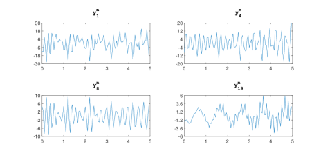
Figure 3: Noisy sampled mixtures ${\mathbf{y}}_{1}^{n}$, ${\mathbf{y}}_{4}^{n}$, ${\mathbf{y}}_{8}^{n}$, ${\mathbf{y}}_{19}^{n}$ $($see Eqs. 69, 70, 71 and 72$)$

A basic problem in signal processing is to assess whether two observed signals involve the same underlying signal “components”. Typically, the component signals manifest themselves with a different amplitude in the observed signals. If moreover the component signals are by themselves unknown, which is the case in many applications, the problem can be very challenging. As a preview, in Fig. 3 it may a priori not be obvious to establish which displayed signals are generated by the same components up to scaling.

One of the possible applications is in underdetermined Blind Source Separation (BSS). In BSS, the task is to recover sources from a set of their linear mixtures [10]. Often, sources are sparsely combined in the observed mixed signals [23], i.e., the number of sources is large but each mixture contains a small number of sources. This means that the mixing matrix is sparse and has many more columns than rows. BSS problems that involve a wide mixing matrix are called underdetermined and are generally much harder to solve than overdetermined BSS problems (involving a mixing matrix that is square or tall). As a preprocessing step one can first try to solve the following multi-label classification problem: mixture $i$ belongs to the same class as mixture $j$ if mixture $i$ is generated by (some of) the sources that appear in mixture $j$. In this way the initial underdetermined BSS problem with many sources can be replaced by a set of smaller overdetermined BSS problems.

In this section we explain how Theorem 4.1 can be used to solve the multi-label classification problem. Our derivation is valid under the assumption that the sources can simultaneously be mapped (i.e., “tensorized”) into low ML rank tensors and that the mapping, so called tensorization, is linear. Such mappings are known [17, 4, 25] for sources that can be modeled as exponential polynomials (Hankelization), rational functions (Löwnerization), and periodic signals (Segmentation), among others. To demonstrate the approach we confine ourselves to exponential polynomials.

To solve the multi-label classification problem, we do not use more prior knowledge about the sources than that they can be (approximately) modeled as exponential polynomials (with a mild bound on the value $L_{s}$ in Eq. 64 that will be introduced in the next subsection).

5.1 Exponential polynomials and Hankelization mapping

A univariate exponential polynomial is a function of the form

(63) $$s(t)=\sum\limits_{f=1}^{F}p_{f}(t)a_{f}^{t},$$

where $p_{1},\dots,p_{F}$ are non-zero polynomials in one variable and $a_{1},\dots,a_{F}\in\mathbb{C}\setminus\{0\}$. Let $T_{s}$ denote the sampling time and let $N$ be the number of sampling points. It can be shown [13, 17] that for any positive integers $I_{1},I_{2},I_{3}$ that sum up to $N+2$ and are greater than or equal to $L_{\mathbf{s}}$, the vector $\mathbf{s}=[s_{1}\ \dots\ s_{N}]^{T}:=[s(0)\ \dots\ s((N-1)T_{s})]^{T}$ can be mapped to an $I_{1}\times I_{2}\times I_{3}$ ML rank-$(L_{\mathbf{s}},L_{\mathbf{s}},L_{\mathbf{s}})$ tensor $\mathcal{S}$, where the value

(64) $$L_{\mathbf{s}}:=F+\sum_{f=1}^{F}\deg p_{f}$$

does not depend on $I_{1}$, $I_{2}$, $I_{3}$. The mapping $H:\mathbf{s}\mapsto\mathcal{S}$, $H:\mathbb{C}^{N}\to\mathbb{C}^{I_{1}\times I_{2}\times I_{3}}$ is given by [13, 17]

$$(\mathcal{S})_{i_{1}i_{2}i_{3}}=s_{i_{1}+i_{2}+i_{3}-2}=s((i_{1}+i_{2}+i_{3}-3)T_{s}),$$

where $1\leq i_{1}\leq I_{1}$, $1\leq i_{2}\leq I_{2}$, $1\leq i_{3}\leq I_{3}$. Since $(\mathcal{S})_{i_{1}i_{2}i_{3}}$ depends only on $i_{1}+i_{2}+i_{3}$, the mapping $H$ was called “Hankelization” in [17]. It is worth noting that if $I_{1}=I_{2}=I_{3}$, then $\mathcal{S}$ is a fully symmetric tensor, implying that ${\mathbf{S}}_{(2,3;1)}={\mathbf{S}}_{(1,3;2)}={\mathbf{S}}_{(1,2;3)}$.

It is clear that $H$ is a linear mapping, so if $\mathbf{y}=[y_{1}\ \dots\ y_{N}]^{T}:=[y(0)\ \dots\ y((N-1)T_{s})]^{T}$ is a linear mixture of sampled sources of the form Eq. 63

(65) $$y(t)=\mathbf{g}_{1}s_{1}(t)+\dots\mathbf{g}_{R}s_{r}(t),\qquad t=0,T_{s},\dots,(N-1)T_{s}$$

and $\min(I_{1},I_{2},I_{3})\geq\max L_{{\mathbf{s}}_{r}}$, then, by Eq. 64,

(66) $$\mathcal{Y}:=H(\mathbf{y})=\mathbf{g}_{1}H(\mathbf{s}_{1})+\dots+\mathbf{g}_{R}H(\mathbf{s}_{R})=\mathbf{g}_{1}\mathcal{S}_{1}+\dots+\mathbf{g}_{R}\mathcal{S}_{R}$$

is a decomposition of $\mathcal{Y}$ into a sum of ML rank-$(L_{\mathbf{s}_{r}},L_{\mathbf{s}_{r}},L_{\mathbf{s}_{r}})$ terms.

5.2 Example

We generate $25$ mixtures

(67) $$y_{j}(t)=\mathbf{g}_{1j}s_{1}(t)+\dots\mathbf{g}_{8j}s_{8}(t),\qquad j=1,\dots,25$$

of $8$ exponential polynomials

$$s_{1}(t)=3\cdot 2^{-\frac{t}{5}}, s_{2}(t)=3\cos(\pi t+\frac{1}{2}), s_{3}(t)=3\cos(2\pi t+2),$$

$$s_{4}(t)=3\cos(3\pi t-2), s_{5}(t)=(5-t)\cos(10\pi t+\frac{1}{2}), s_{6}(t)=(5-t)\cos(12\pi t-\frac{3}{2}),$$

$$s_{7}(t)=t\cos(8\pi t+1), s_{8}(t)=t\cos(14\pi t-\frac{1}{2}).$$

The coefficients $\mathbf{g}_{ij}$ are generated randomly so that for each $j=1,\dots,25$ at least three and at most six of $\mathbf{g}_{1j},\dots,\mathbf{g}_{8j}$ are zero. The nonzero coefficients $\mathbf{g}_{ij}$ are randomly chosen from $[-2.5,-0.5]\cup[0.5,2.5]$. We thus obtain that

(68) $$[y_{1}(t)\ \dots y_{25}(t)]=[s_{1}(t)\ \dots s_{8}(t)]\mathbf{G},$$

where $\mathbf{G}=(\mathbf{g}_{ij})$ is an $8\times 25$ sparse matrix. The nonzero pattern of $\mathbf{G}$ is shown in Fig. 1.

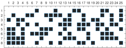
Figure 1: The nonzero pattern of the matrix $\mathbf{G}$.

By way of example, the mixtures $y_{1}(t)$, $y_{4}(t)$, $y_{8}(t)$, and $y_{19}(t)$ were generated as

(69) $$y_{1}(t)= 2.22s_{3}(t) -1.95s_{5}(t) -2.38s_{6}(t) -2.39s_{7}(t)\phantom{,} +1.77s_{8}(t),$$

(70) $$y_{4}(t)= -0.55s_{3}(t) -2.07s_{5}(t) +0.50s_{6}(t) +2.41s_{7}(t)\phantom{,} -1.90s_{8}(t),$$

(71) $$y_{8}(t)= +1.16s_{5}(t) +0.94s_{6}(t) +1.35s_{7}(t),$$

(72) $$y_{19}(t)= 0.69s_{3}(t) -0.68s_{8}(t).$$

We consider a noisy sampled (with $T_{s}=0.05$ and $N=100$) version of Eq. 68:

(73) $$[{\mathbf{y}}_{1}^{n}\ \dots\ {\mathbf{y}}_{25}^{n}]:=[\mathbf{y}_{1}\ \dots\ \mathbf{y}_{25}]+\sigma\mathbf{N}=[\mathbf{s}_{1}\ \dots\mathbf{s}_{8}]\mathbf{G}+\sigma\mathbf{N},$$

in which the entries of the $100\times 25$ matrix $\mathbf{N}$ are independently drawn from the standard normal distribution $N(0,1)$ and $\sigma=0.1\frac{\|[\mathbf{y}_{1}\ \dots\ \mathbf{y}_{25}]\|_{F}}{\|\mathbf{N}\|_{F}}$, where $\|\cdot\|_{F}$ denotes the Frobenius norm. The sampled sources $\mathbf{s}_{1},\dots,\mathbf{s}_{8}$ and noisy sampled mixtures ${\mathbf{y}}_{1}^{n}$, ${\mathbf{y}}_{4}^{n}$, ${\mathbf{y}}_{8}^{n}$, ${\mathbf{y}}_{19}^{n}$ are shown in Figs. 2 and 3, respectively.

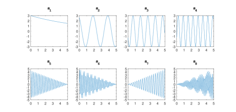
Figure 2: Sampled source signals ${\mathbf{s}}_{1},\dots,{\mathbf{s}}_{8}$.

.

We now use Theorem 4.1 to verify whether the pair of mixtures $(y_{i}(t),y_{j}(t))$ is generated by the same subset of sources, $1\leq i,j\leq 25$, $i\neq j$. For visualization purposes it is convenient to associate the mixtures $y_{1}(t),\dots,y_{25}(t)$ with vertices of a directed graph: a directed edge from vertex $i$ to vertex $j$ indicates that $y_{i}(t)$ is generated by sources that also appear in $y_{j}(t)$. For instance, the subgraph corresponding to the mixtures $y_{1}(t)$, $y_{4}(t)$, $y_{8}(t)$, and $y_{19}(t)$ is shown in Fig. 4a. In this example we show how to recover the overall graph in Fig. 4b based only on the (observed) vectors ${\mathbf{y}}_{1}^{n},\dots,{\mathbf{y}}_{25}^{n}$ and without estimating ${\mathbf{s}}_{1},\dots,{\mathbf{s}}_{8}$.

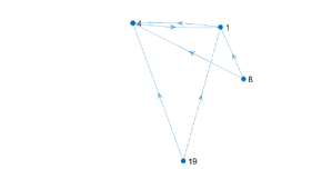
(a)

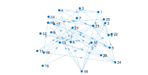
(b)

Figure 4: The subgraph corresponding to the mixtures $y_{1}(t)$, $y_{4}(t)$, $y_{8}(t)$, $y_{19}(t)$ $($left$)$ and the graph corresponding to all mixtures $y_{1}(t),\dots,y_{25}(t)$ $($right$)$; a directed edge from vertex $i$ to vertex $j$ indicates that mixture $y_{i}(t)$ is generated by sources that also appear in mixture $y_{j}(t)$.

Let $H:\mathbb{C}^{100}\to\mathbb{C}^{34\times 34\times 34}$ denote the Hankelization mapping. By Eqs. 66 and 73, we have that

$${\mathcal{Y}}_{i}^{n}:=H({\mathbf{y}}_{i}^{n})=\mathbf{g}_{i1}H(\mathbf{s}_{1})+\dots+\mathbf{g}_{i8}H(\mathbf{s}_{8})+\sigma H(\mathbf{n}_{i})=\mathbf{g}_{i1}\mathcal{S}_{1}+\dots+\mathbf{g}_{18}\mathcal{S}_{R}+\sigma H(\mathbf{n}_{i})$$

is an approximate decomposition of ${\mathcal{Y}}_{i}^{n}$ into a sum of ML rank-$(L_{\mathbf{s}_{r}},L_{\mathbf{s}_{r}},L_{\mathbf{s}_{r}})$ terms. One can easily verify that the exact values of $L_{\mathbf{s}_{1}},\dots,L_{\mathbf{s}_{8}}$ are $1,2,2,2,4,4,4,4$, respectively. For instance, since

$$s_{8}(t)=t\frac{1}{2}(e^{(14\pi t-0.5)i}+e^{-(14\pi t-0.5)i})=(\frac{1}{2}e^{-0.5i}t^{1})e^{14\pi t}+(\frac{1}{2}e^{0.5i}t^{1})e^{-14\pi t},$$

we get, by Eq. 64, that $L_{\mathbf{s}_{8}}=2+(1+1)=4$. On the other hand, it can be verified that although the tensors $\mathcal{S}_{5},\dots,\mathcal{S}_{8}$ are ML rank-$(4,4,4)$, they can be approximated by ML rank-$(2,2,2)$ tensors with a relative error less than $0.061$, which is below the noise level.

To verify whether $y_{i}(t)$ is generated by sources that appear in $y_{j}(t)$, it is sufficient to show that ${\mathcal{Y}}_{i}^{n}$ is generated by ML rank terms that appear in ${\mathcal{Y}}_{j}^{n}$, which, by Theorem 4.1, is reduced to verifying that the column space of ${\mathbf{Y}_{i}^{n}}_{(2,3;1)}$ is contained in the column space of ${\mathbf{Y}_{j}^{n}}_{(2,3;1)}$. To compare the column spaces we proceeded as follows. For each $i=1,\dots,25$ we computed the first $r_{i}$ singular vectors $\mathbf{u}_{i1},\dots,\mathbf{u}_{ir_{i}}$ of ${\mathbf{Y}_{i}^{n}}_{(2,3;1)}$, where the rank $r_{i}$ of ${\mathbf{Y}_{i}^{n}}_{(2,3;1)}$ was estimated as the largest index $k$ such that the ratio of the $k$th and the $(k+1)$st singular value of ${\mathbf{Y}_{i}^{n}}_{(2,3;1)}$ is greater than a certain threshold $\tau$. (We chose $\tau=2.3$.) Then for all $i,j=1,\dots,25$ and $i\neq j$ we concluded that the column space of ${\mathbf{Y}_{i}^{n}}_{(2,3;1)}$ is contained in the column space of ${\mathbf{Y}_{j}^{n}}_{(2,3;1)}$ if the $(r_{j}+1)$st singular value of the matrix $[\mathbf{u}_{i1}\ \dots\ \mathbf{u}_{ir_{i}}\ \mathbf{u}_{j1}\ \dots\ \mathbf{u}_{jr_{j}}]$ was less than $0.1$ (and in this case we plotted the directed edge from vertex $i$ to vertex $j$). The resulting directed graph is shown in Fig. 4b. The same graph can be obtained directly from the nonzero pattern of the matrix $\mathbf{G}$ which means that all $43$ (out of the possible $600$) edges of the graph were detected correctly and no superfluous edges were added.

6 Conclusion

An obvious requirement for a tensor $\mathcal{B}$ to be the sum of (possibly scaled) terms from the decomposition of a tensor $\mathcal{A}$, is that its column (row, fiber, …) space is a subspace of the corresponding space of tensor $\mathcal{A}$. Formally, this means that $\operatorname{row}({\mathbf{B}}_{({n}^{c};n)})\subseteq\operatorname{row}({\mathbf{A}}_{({n}^{c};n)})$ should hold for all $n\in\{1,\dots,N\}$. However, this is only a necessary condition. Switching to the column spaces, we have shown in this paper that

(74) $$\operatorname{col}({\mathbf{B}}_{({n}^{c};n)})\subseteq\operatorname{col}({\mathbf{A}}_{({n}^{c};n)}),\qquad n\in\{1,\dots,N\}$$

is a sufficient condition for $\mathcal{B}$ to be generated by (possibly scaled) terms from the decomposition of $\mathcal{A}$. The number or terms and their “type” (namely, their ML rank) follow from the analysis as well. As the derivation relies only on linear algebra, it bypasses the typical difficulties in the computation of CPD and BTD, such as NP-hardness and possible ill-conditioning. We believe that this paper introduces a new tool that will prove important for tensor-based pattern recognition and machine learning, in a similar way as (explicit) tensor decompositions have proven to be fundamental tools for data analysis. We have illustrated the practical use of the new tool in a new clustering-based scheme for sparse underdetermined BSS.

An interesting topic of further study would be to investigate partially shared structure of $\mathcal{A}$ and $\mathcal{B}$, in the sense that $\mathcal{A}$ and $\mathcal{B}$ share some but not all terms. We will also derive more detailed information from the actual principal angles and associated directions between the subspaces obtained from $\mathcal{A}$ and $\mathcal{B}$. Another topic of further study is the generalization to “flower”, “butterfly” and related decompositions [3, 4, 28].

References

- [1] C. Beltrán, P. Breiding, and N. Vannieuwenhoven, The average condition number of most tensor rank decomposition problems is infinite, arxiv:1903.05527, (2019).
- [2] C. Beltrán, P. Breiding, and N. Vannieuwenhoven, Pencil-based algorithms for tensor rank decomposition are not stable., SIAM J. Matrix Anal. Appl., 40 (2019), pp. 739–773.
- [3] M. Boussé, O. Debals, and L. De Lathauwer, Tensor-based large-scale blind system identification using segmentation, IEEE Transactions on Signal Processing, 65 (2017), pp. 5770–5784.
- [4] M. Boussé, O. Debals, and L. De Lathauwer, A tensor-based method for large-scale blind source separation using segmentation, IEEE Transactions on Signal Processing, 65 (2017), pp. 346–358.
- [5] P. Breiding and N. Vannieuwenhoven, On the average condition number of tensor rank decompositions., IMA Journal of Numerical Analysis, (2019).
- [6] R. Bro, R. A. Harshman, N. D. Sidiropoulos, and M. E. Lundy, Modeling multi-way data with linearly dependent loadings, Journal of Chemometrics, 23 (2009), pp. 324–340.
- [7] L. Chiantini, G. Ottaviani, and N. Vannieuwenhoven, An algorithm for generic and low-rank specific identifiability of complex tensors, SIAM J. Matrix Anal. Appl., 35 (2014), pp. 1265–1287.
- [8] L. Chiantini, G. Ottaviani, and N. Vannieuwenhoven, Effective criteria for specific identifiability of tensors and forms, SIAM J. Matrix Anal. Appl., 38 (2017), pp. 656–681.
- [9] A. Cichocki, D. Mandic, C. Caiafa, A.-H. Phan, G. Zhou, Q. Zhao, and L. De Lathauwer, Tensor decompositions for signal processing applications. From two-way to multiway component analysis, IEEE Signal Process. Mag., 32 (2015), pp. 145–163.
- [10] P. Comon and C. Jutten, eds., Handbook of Blind Source Separation, Independent Component Analysis and Applications, Academic Press, Oxford, UK, 2010.
- [11] C. W. Curtis, Linear Algebra: An Introductory Approach, Springer, New York, NY, 1984.
- [12] L. De Lathauwer, Decompositions of a higher-order tensor in block terms — Part II: Definitions and uniqueness, SIAM J. Matrix Anal. Appl., 30 (2008), pp. 1033–1066.
- [13] L. De Lathauwer, Blind separation of exponential polynomials and the decomposition of a tensor in rank- terms, SIAM J. Matrix Anal. Appl., 32 (2011), pp. 1451–1474.
- [14] L. De Lathauwer, Characterizing higher-order tensors by means of subspaces, STADIUS Res. Division, Dept. Elect. Eng., Katholieke Univ. Leuven, Leuven, Belgium, Tech. Rep. 11-32, (2011).
- [15] L. De Lathauwer and A. de Baynast, Blind deconvolution of DS-CDMA signals by means of decomposition in rank- terms, IEEE Trans. Signal Process., 56 (2008), pp. 1562–1571.
- [16] L. De Lathauwer, B. De Moor, and J. Vandewalle, A multilinear singular value decomposition, SIAM J. Matrix Anal. Appl., 21 (2000), pp. 1253–1278.
- [17] O. Debals, Tensorization and applications in blind source separation, PhD thesis, Faculty of Engineering, KU Leuven (Leuven, Belgium), August 2017.
- [18] O. Debals, M. Van Barel, and L. De Lathauwer, Löwner-based blind signal separation of rational functions with applications, IEEE Trans. Signal Process., 64 (2016), pp. 1909–1918.
- [19] I. Domanov and L. De Lathauwer, On the uniqueness of the canonical polyadic decomposition of third-order tensors — Part I: Basic results and uniqueness of one factor matrix, SIAM J. Matrix Anal. Appl., 34 (2013), pp. 855–875.
- [20] I. Domanov and L. De Lathauwer, On the uniqueness of the canonical polyadic decomposition of third-order tensors — Part II: Overall uniqueness, SIAM J. Matrix Anal. Appl., 34 (2013), pp. 876–903.
- [21] I. Domanov and L. De Lathauwer, On uniqueness and computation of the decomposition of a tensor into multilinear rank- terms, arXiv:1808.02423, (2018).
- [22] I. Domanov, N. Vervliet, and L. De Lathauwer, Decomposition of a tensor into multilinear rank- terms, Internal Report 18-51, ESAT-STADIUS, KU Leuven (Leuven, Belgium), (2018).
- [23] D. Donoho, Sparse components of images and optimal atomic decompositions, Constructive Approximation, 17 (2001), pp. 353–382.
- [24] R. A. Horn and C. R. Johnson, Matrix Analysis, Cambridge University Press, Cambridge, 2012.
- [25] B. N. Khoromskij, Tensor Numerical Methods in Scientific Computing, De Gruyter, 2018.
- [26] T. G. Kolda and B. W. Bader, Tensor decompositions and applications, SIAM Review, 51 (2009), pp. 455–500.
- [27] N. D. Sidiropoulos, L. De Lathauwer, X. Fu, K. Huang, E. E. Papalexakis, and C. Faloutsos, Tensor decomposition for signal processing and machine learning, IEEE Trans. Signal Process., 65 (2017), pp. 3551–3582.
- [28] L. Sorber, M. Van Barel, and L. De Lathauwer, Optimization-based algorithms for tensor decompositions: canonical polyadic decomposition, decomposition in rank-(,,1) terms and a new generalization, SIAM J. Optim., 23 (2013), pp. 695–720.
- [29] L. R. Tucker, The extension of factor analysis to three-dimensional matrices, in Contributions to Mathematical Psychology, H. Gulliksen and N. Frederiksen, eds., Holt, Rinehart & Winston, New York, 1966.
- [30] L. R. Tucker, Some mathematical notes on three-mode factor analysis, Psychometrika, 31 (1966), pp. 279–311.
- [31] F. Van Eeghem, O. Debals, and L. De Lathauwer, Tensor similarity in two modes, IEEE Transactions on Signal Processing, 66 (2018), pp. 1273–1285.