Thermodynamic costs of Turing Machines

Abstract

Turing Machines (TMs) are the canonical model of computation in computer science and physics. We combine techniques from algorithmic information theory and stochastic thermodynamics to analyze the thermodynamic costs of TMs. We consider two different ways of realizing a given TM with a physical process. The first realization is designed to be thermodynamically reversible when fed with random input bits. The second realization is designed to generate less heat, up to an additive constant, than any realization that is computable (i.e., consistent with the physical Church-Turing thesis). We consider three different thermodynamic costs: the heat generated when the TM is run on each input (which we refer to as the “heat function”), the minimum heat generated when a TM is run with an input that results in some desired output (which we refer to as the “thermodynamic complexity” of the output, in analogy to the Kolmogorov complexity), and the expected heat on the input distribution that minimizes entropy production. For universal TMs, we show for both realizations that the thermodynamic complexity of any desired output is bounded by a constant (unlike the conventional Kolmogorov complexity), while the expected amount of generated heat is infinite. We also show that any computable realization faces a fundamental tradeoff between heat generation, the Kolmogorov complexity of its heat function, and the Kolmogorov complexity of its input-output map. We demonstrate this tradeoff by analyzing the thermodynamics of erasing a long string.

I Introduction

The relationship between thermodynamics and information-processing has been an important area of research since at least the 1960s, when Landauer proposed that any process which erases a bit of information must release at least $kT\ln 2$ of heat into its environment bril53 ; bril62 ; landauer1961irreversibility ; szilard1964decrease ; zure89a ; zure89b ; bennett1982thermodynamics ; lloyd1989use ; dunkel2014thermodynamics ; roldan2014universal ; lloyd2000ultimate ; fredkin1990informational ; toffoli1990invertible ; leff2014maxwell ; maroney2009generalizing ; turgut_relations_2009 . This research has greatly benefited from the dramatic progress in nonequilibrium statistical physics in the past few decades, in particular the development of trajectory-based and stochastic thermodynamics van2013stochastic ; van2015ensemble ; seifert2012stochastic . These developments now permit us to quantify and analyze heat, work, entropy production and other thermodynamic properties of individual trajectories in far-from-equilibrium systems. They have also have led to a much deeper understanding of the relationship between thermodynamics and information processing, both for information erasure berut2012experimental ; diana2013finite ; zulkowski2014optimal ; jun2014high ; ciliberto2017experiments ; barato2014unifying and other more elaborate computations wiesner2012information ; sagawa2012fluctuation ; still2012thermodynamics ; prokopenko2013thermodynamic ; prokopenko2014transfer ; roldan2014universal ; koski2014experimental ; parrondo2015thermodynamics ; wolpert_book_2018 ; wolpert_thermo_comp_review_2019 ; Boyd2018thesis ; strasberg2015thermodynamics ; grochow_wolpert_sigact2018 ; riechers_thermo_comp_book_2018 ; wolpert_book_2018 ; ouldridge_thermo_comp_book_2018 ; strasberg2015thermodynamics .

In this paper we extend this line of research by deriving new results on the thermodynamic costs of performing general computations, as formalized by the notion of Turing machines (TMs). A TM is an abstraction of a conventional modern computer, which run programs written in a conventional programming language (C, Python, etc.) sipser2006introduction ; hopcroft2000jd ; livi08 ; grunwald2004shannon ; arora2009computational ; savage1998models . A TM reads an input string of arbitrary length (a “program”) and runs until it produces an output string. In the same way that any modern computer can simulate other computers (e.g., via an emulator), there exist an important class of TMs called universal Turing Machines (UTMs), each of which is able to simulate the operation of any other TM.

TMs are a keystone of the theory of computation moore2011nature , and touch upon several foundational issues that lie at the intersection of mathematics and philosophy, such as whether $\mathsf{P}=\mathsf{NP}$ and Gödel’s incompleteness theorems aaronson2013philosophers . Their importance is partly due to the celebrated Church-Turing thesis, which postulates that any function that can be computed by a sequence of formal operations can also be computed by some TM turing1948intelligent ; church1937review ; sep-computation-physicalsystems . For this reason, in computer science, a function is called computable if and only if it can be carried out by a TM livi08 . TMs also play important roles in many facets of modern physics. For instance, TMs are used to formalize the difference between easy and hard computational problems in quantum computing cubitt2015undecidability ; cubitt2012extracting ; deutsch1985quantum ; benioff1982quantum ; nielsen2010quantum . There has also been some speculative, broader-ranging work on whether the foundations of physics may be restricted by some of the properties of TMs barrow2011godel ; aaro05 . Finally, there has been extensive investigation of the physical Church-Turing thesis, which states that any function that can be implemented by a physical process can also be computed with a TM gandy1980church ; wolfram1985undecidability ; deutsch1985quantum ; geroch1986computability ; nielsen1997computable ; arrighi2012physical ; piccinini2011physical ; pitowsky1990physical ; ziegler2009physically ; cubitt2015undecidability ; moore1990unpredictability ; da1991undecidability ; kanter1990undecidability ; kieu2003computing ; copeland2002hypercomputation .

One of the most important concepts in the theory of TMs is Kolmogorov complexity. The Kolmogorov complexity of a string $y$, written as $K(y)$, is the length of the shortest input program which causes a UTM to produce $y$ as the output (formal definitions are provided in Section II.2). The Kolmogorov complexity of a string $y$ captures the amount of randomness in $y$, because a string with a non-random pattern can be produced by a short input program. For example, the string containing the first billion digits of $\pi$ can be generated by running a very short program, and so has small Kolmogorov complexity. In contrast, for a random string $y$ without any patterns, the shortest program that produces $y$ is a program of the type $\text{``}\texttt{print `}y\texttt{`}\text{''}$, which has about the same length as $y$. An important variant of Kolmogorov complexity is the conditional Kolmogorov complexity of $y$ given $x$, written $K(y|x)$, which is the length of the shortest program which causes a UTM to produce $y$ as output, when the UTM is provided with $x$ as an additional input. Kolmogorov and conditional Kolmogorov complexity have many formal connections with entropy and conditional entropy from Shannon’s information theory grunwald2004shannon , and are studied in a field called Algorithmic Information Theory (AIT) livi08 ; chaitin2004algorithmic .

In this paper, we combine techniques from AIT and stochastic thermodynamics to analyze the thermodynamics of TMs. We imagine a discrete-state physical system that is coupled to a heat bath at temperature $T$, and which evolves under the influence of a driving protocol. We identify the initial and final states of the physical system with the logical inputs and outputs of some TM, so that the dynamics over the states of the physical system corresponds to a computation performed by the TM. We refer to a physical process that is consistent with the laws of thermodynamics and whose dynamics correspond to the input-output map of a TM as a realization of that TM.

We derive numerous results that concern the thermodynamic properties of realizations of TMs. The core underlying idea behind these results is that the logical properties a given TM (such as the structure of the TM’s input-output map, or the Kolmogorov complexity of its inputs and outputs) provide constraints on the thermodynamic costs incurred by realizations of that TM (such as the amount of heat those realizations generate). Some of our results relate logical properties and thermodynamic costs at the ensemble level (i.e., relative to a probability distribution over computational trajectories of a TM), thereby building on the thermodynamic analysis initiated by Landauer and others. In addition to these, many of our results also relate logical properties and thermodynamic costs at the level of individual computational trajectories (i.e., individual runs of the TM), which goes beyond most existing research on thermodynamics of computation.

I.1 Summary of results

We investigate three different kinds of thermodynamic costs for a given realization of a TM:

(1) The amount of heat that is generated by running the realization of a given (univeral or non-universal) TM on each individual input $x$. We refer to the map from inputs to their associated heat values as the heat function of the TM’s realization, and write it as $Q(x)$.

(2) The minimal amount of heat generated by running the realization of a given TM on some individual input that results in a desired output $y$. Here we assume that the TM is universal, so that it can in principle produce any output. This second cost is a function of the desired output $y$, rather than of the input $x$, and can be viewed as a thermodynamic analog of conventional Kolmogorov complexity. For this reason, we refer to this cost as the thermodynamic complexity of $y$.

(3) The ensemble-level expected heat $\langle Q\rangle$ generated by the realization of a TM, evaluated for the input distribution that minimizes entropy production (EP). For this cost, we again focus on the case of universal TMs.

In general, there are many physical processes that are realizations of the same TM, which can have different thermodynamic costs from one another. In this paper we consider the above three thermodynamic costs for two important types of realizations. The first realization we consider, which is called the coin-flipping realization, is constructed to be thermodynamically reversible when input programs are sampled from the “coin-flipping” distribution $p(x)\propto 2^{-\ell(x)}$, where $\ell(x)$ indicates the length of string $x$. This input distribution arises by feeding random bits into a TM (hence its name) and plays a fundamental role in AIT.

We show that the heat function of the coin-flipping realization of a given TM is proportional to $\ell(x)$ minus a “correction term” which reflects the logically irreversibility of the input-output map computed by the TM. Importantly, when the realized TM is a universal TM $U$, this correction term can be related to the Kolmogorov complexity of the output of $U$ on input $x$. In this case, the heat function is given by

$$Q_{\mathrm{coin}}(x)=kT\ln 2\,[\ell(x)-K(\phi_{U}(x))]+O(1),$$ (1)

where $\phi_{U}(x)$ indicates the output of $U$ on input $x$, and $O(1)$ indicates equality up to an additive constant independent of $x$ (see Section I.3 for a formal definition). Thus, up to an additive constant, the heat generated by running input $x$ on the coin-flipping realization of some UTM $U$ is proportional to the excess length of the input program $x$, over and above the length of the shortest program for $U$ that produces the same output as $x$.

It follows from Eq. 1 that if $x$ is the shortest program for $U$ that produces output $\phi_{U}(x)$, then $Q_{\mathrm{coin}}(x)=O(1)$. This means that by running the shortest program $x$ that produces some desired $y$ as output, one can produce that $y$ for an amount of heat that is bounded by a constant. Thus, the thermodynamic complexity for the coin-flipping realization is a bounded function, unlike the Kolmogorov complexity, which grows arbitrarily large livi08 . On the other hand, we also show that when inputs are sampled from the coin-flipping distribution, the expected heat $\langle Q\rangle$ generated by the coin-flipping realization of a UTM is infinite. This holds even though the heat necessary to run the UTM on any given input $x$ is finite.

The second realization we analyze is inspired by the physical Church-Turing thesis. To begin, we refer to a realization of a TM with heat function $Q$ as a computable realization if the function $x\mapsto Q(x)/kT$ is computable (i.e., there exist some TM that takes as input any desired $x$ and outputs the corresponding heat value $Q(x)$ in units of $kT$). Under common interpretations of the physical Church-Turing thesis deutsch1985quantum ; wolfram1985undecidability ; geroch1986computability ; pitowsky1990physical ; nielsen1997computable ; sep-computation-physicalsystems , any realization that is actually constructable in the real-world must be computable; in other words, a non-computable realization is a hypothetical physical process which does not violate any laws of thermodynamics, but which nonetheless cannot be constructed because of computational constraints. Motivated by these observations, we define the so-called dominating realization of a TM $M$ to be “optimal” in the following sense: the heat it generates on any input $x$ is smaller than the heat generated by any computable realization of $M$ on $x$, up to an additive constant which does not depend on $x$. The heat function of the dominating realization is proportional to the conditional Kolmogorov complexity of the output given the input,

$$Q_{\mathrm{dom}}(x)=kT\ln 2\cdot K(x|\phi_{M}(x)),$$ (2)

where $\phi_{M}(x)$ indicates the output of TM $M$ on input $x$. We show that this heat function is smaller than the heat function $Q$ of any computable realization of $M$,

$$Q_{\mathrm{dom}}(x)\leq Q(x)+O(1).$$ (3)

Note that this result holds whether or not $M$ is a UTM.

For the special case where $M$ is a UTM, we show that for any desired output $y$, the thermodynamic complexity of $y$ under the dominating realization is bounded by a constant that is independent of $y$, just like for the coin-flipping realization. Moreover, for the dominating realization there is a simple scheme for choosing the input $x$ that will produce any desired output $y$ with a bounded amount of heat. This differs from the coin-flipping realization, where one must know the shortest program that generates $y$ in order to produce $y$ with a bounded amount of heat (in general, finding the shortest program to produce a given output $y$ is not computable).

Finally, we consider the expected heat that is generated by the dominating realization, given some probability distribution over input programs. A natural input distribution to consider is the one that minimizes the entropy production of the dominating realization. As for the coin-flipping realization, we show that the expected heat across inputs sampled from this distribution is infinite.

There are two important caveats concerning the dominating realization. First, while the dominating realization is better than any computable realization, in the sense of Eq. 3, it itself is not computable. This is because its heat function is defined in terms of the conditional Kolmogorov complexity, which is not a computable function. Nonetheless, as we discuss below, one can always define a sequence of computable realizations whose heat functions approach $Q_{\mathrm{dom}}$ from above. Thus, the dominating realization presents a fundamental bound on the heat generation of computable realizations, and this bound is achievable in the limit.

Second, for a given TM $M$, Eq. 3 states that the heat generated by the dominating realization on input $x$, $Q_{\mathrm{dom}}(x)$, is smaller than the heat generated by any computable realization, $Q(x)$, up to an additive constant that does not depend on $x$. This additive constant, however, can depend on the particular alternative realization of $M$ that is being compared, i.e., on the choice of comparison heat function $Q$. In fact, depending on the alternative realization, that additive constant can be arbitrarily large and negative. This means that for a given TM $M$ and some particular choice of input program $x$, there may exist alternative realizations of $M$ that generate arbitrarily less heat than the dominating realization. It turns out, however, that the difference between $Q_{\mathrm{dom}}(x)$ and $Q(x)$ is upper bounded by the sum of the Kolmogorov complexity of the input-output function $\phi_{M}$ and the Kolmogorov complexity of the comparison heat function $Q$. Using this result, we show that any computable realization that produces output $y$ from input $x$ faces a fundamental cost of $K(x|y)$, which can be paid either by producing a large amount of heat, by computing an input-output map with high complexity, or by having a heat function with high complexity.

The paper is laid out as follows. In the following subsections, we review relevant prior work and introduce notation. In Section II, we define TMs and review some relevant results from AIT. In Section III, we review the basics of statistical physics, and discuss how a TM can be implemented as a physical system. We present our main results on the coin-flipping and dominating realizations in Section IV and Section V. In Section VI, we demonstrate the tradeoff between heat and complexity by analyzing the thermodynamics of erasing a long string. In the last section we discuss potential directions for future research.

I.2 Prior work on thermodynamics of TMs

Some of the earliest work on the thermodynamics of TMs focused on TMs with deterministic and logically reversible dynamics benn73 ; bennett1989time . Logically reversible TMs can perform computations without generating any heat or entropy production, at the cost of having to store additional information in their output, which logically irreversible TMs do not need to store. Due to the thermodynamic costs that would arise in re-initializing that extra stored information, there are some subtleties in calculating the thermodynamic cost of running a “complete cycle” of any logically reversible TM wolpert_thermo_comp_review_2019 . (See also sagawa2014thermodynamic ; sagawa2019second for a discussion of the relationship between thermodynamic and logical reversibility.) Logically reversible TMs form a special subclass of TMs, and require special definitions of universality morita_theory_2017 . In this work, we focus on the thermodynamics of general-purpose TMs, whose computations will generally be logically irreversible. However, we will sometimes also discuss how our results apply in the logically reversible case.

More recently, strasberg2015thermodynamics analyzed the thermodynamics of logically reversible TMs with stochastic forward-backward dynamics along a computational trajectory, which causes the state of the TM to become more uncertain with time. This model incurs non-zero entropy production, even though each computational trajectory encodes a logically reversible computation. Note that this entropy production could in principle be made arbitrarily small by driving the TM forward with momentum (e.g., by coupling it to a large flywheel). In this work, we will ignore possible stochasticity in the progression of a TM along its computational trajectory.

Finally, there has been recent work which interprets the coin-flipping distribution over strings $x$, as defined in Section IV, as a “Boltzmann distribution” induced by the “energy function” $\ell(x)$ baez2012algorithmic . Doing this allows one to formulate a set of equations concerning TMs that are formal analogs of Maxwell’s relations for equilibrium thermodynamic systems.

In our own earlier work, we began to analyze the thermodynamic complexity of computing desired outputs, focusing on the coin-flipping realization and a three-tape UTM wolpert_arxiv_beyond_bit_erasure_2015 . We first showed explicitly how to construct a system that is thermodynamically reversible for the coin-flipping distribution, and then derived the associated heat function. We showed that for this realization, the minimal amount of heat needed to compute any given output $y$ equals the Kolmogorov complexity of $y$, plus what we characterized as a “correction term”. In other, more recent work, we rederived these results using stochastic thermodynamics and single-tape machines wolpert_book_review_chap_2019 .

In this paper, we extend this earlier work on the coin-flipping realization. For simplicity, we consider the thermodynamics of systems that implement the entire computation of a given UTM in some fixed time interval. (In contrast, our earlier work considered systems that implement a given UTM’s update function iteratively, taking varying amounts of time to halt, depending on the input to the UTM.) We then go further, and use Levin’s Coding theorem to show that the thermodynamic complexity of the coin-flipping realization is bounded, even though the conventional Kolmogorov complexity function is not. We also extend this earlier work by showing that the coin-flipping realization generates infinite expected heat when inputs are sampled from the coin-flipping distribution.

The other main contributions of this paper concern the thermodynamic costs of the dominating realization. These results are related to a series of ground-breaking papers begun by Zurek zure89a ; zure89b ; li1992mathematical ; bennett1993thermodynamics ; bennett1998information ; caves1990entropy ; caves1993information ; baumeler2019free ; zurek1990algorithmic . Those papers were generally written before the widespread adoption of trajectory-based analyses of thermodynamics van2015ensemble , and contained a semiformal argument that computing an output string $y$ from an input $x$ has a minimal “thermodynamic cost” of at least $K(x|y)$. Even though that semiformal argument is quite different from our analysis, the same “thermodynamic cost” function also appears in our analysis of the dominating realization. We discuss connections between our results and this earlier work in more detail in Section VI.

I.3 Notation

We use uppercase letters, such as $X$ and $Y$, to indicate random variables. We use lowercase letters, like $x$ and $y$, to indicate their outcomes. We use $p_{X}$ to indicate a probability distribution over random variable $X$, and $p_{X|Y}$ to indicate a conditional probability distribution of random variable $X$ given random variable $Y$. We also use $p_{X|Y=y}$ to indicate the probability distribution of $X$ conditioned on one particular outcome $Y=y$. Finally, we use $\operatorname{supp}p_{X}$ to indicate the support of distribution $p_{X}$, and notation like $\langle f(X)\rangle_{p_{X}}=\sum_{x}p_{X}(x)f(x)$ to indicate expectations.

A partial function $f:A\to B$ is a map from some subset of $A$, which is called the domain of definition of $f$, into $B$. We write $\mathrm{dom\,}f\subseteq A$ to indicate the domain of definition of $f$, and $\mathrm{img\,}f:=\{f(a):a\in\mathrm{dom\,}f\}$ to indicate the image of $f$. The value of $f(a)$ is undefined for any $a\not\in\mathrm{dom\,}f$.

For any set $A$, we use $A^{*}$ to indicate the set of finite strings of elements from $A$. We use $A^{\infty}$ to indicate the set of infinite strings of elements from $A$. In particular, $\{0,1\}^{*}$ indicates the set of all finite binary strings. Note that for any finite $A$, $A^{*}$ is a countably infinite set.

The Kronecker delta is indicated by $\delta(\cdot,\cdot)$. We sometimes write $\delta_{x}$ to indicate a delta-function probability distribution over outcome $x$ of random variable $X$, $\delta_{x}(x^{\prime})=\delta(x,x^{\prime})$.

We use standard asymptotic notation, such as $f(x)=g(x)+O(1)$, which indicates that $|f(x)-g(x)|\leq\kappa$ for some $\kappa\in\mathbb{R}$ and all $x$. Similarly, notation like $f(x)\leq g(x)+O(1)$ indicates that $f(x)-g(x)\leq\kappa$ for some $\kappa\in\mathbb{R}$ and all $x$.

II Background on Turing Machines and AIT

II.1 Turing Machines

In its canonical definition, a TM comprises three variables, and a rule for their joint dynamics. First, there is a tape variable whose state is a semi-infinite string $s\in A^{\infty}$, where $A$ is a finite set of tape symbols which includes a special blank symbol. Second, there is a pointer variable $v\in\{1,2,3,\dots\}$, which is interpreted as specifying a “position” on the tape (i.e., an index into the infinite-dimensional vector $s$). Finally, there is a head variable $h$ whose state belongs to a finite set, which includes a specially designated start state and a specially designated halt state.

The TM starts with its head in the start state, the pointer set to position 1, and its tape containing some finite string of non-blank symbols, followed by blank symbols. The joint state of the tape, pointer, and head evolves over time according to a discrete-time update function. If during that evolution the head ever enters its halt state, that is interpreted as the computation being completed. If and when the computation completes, we say that the TM has then computed its output, which is specified by the state of its tape at that time. Importantly, for some inputs, a TM might never complete its computation, i.e., it may go into an infinite loop and never enter the halt state. The operation of a TM is illustrated in a schematic way in Fig. 1. A more formal definition of a TM and the update function is provided in Appendix A.

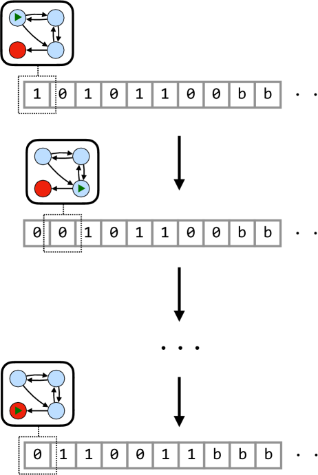
Figure 1: A TM performing a computation. The update function is applied over a sequence of steps, causing the finite-state head (rounded box, states are colored circles) to move along an infinite tape of symbols (b indicates a special “blank” symbol). During each step, the head can read/write the tape symbol in the current position, move left or right along the tape, and change its current state (green triangle). The computation completes if and when the head reaches its halt state (red circle).

There many other variants of TMs that have been considered in the literature, including ones with multiple tapes and multiple heads. However, all of these variants are computationally equivalent: any computation that can be carried out with a particular TM variant can also be carried out with some TM that possesses a single tape and a single head sipser2006introduction ; papadimitriou2003computational ; wolpert_thermo_comp_review_2019 .

For simplicity of analysis, we make two assumptions about the TMs analyzed in this paper, none of which affect the computational capabilities of the TMs. First, we assume that the tape alphabet $A$ contains the binary symbols $0$ and $1$, and that these are the only non-blank symbols present on the tape at the beginning of the computation. Second, we assume that any TM we consider is designed so that, if and when it reaches a halt state, its tape will contain a string from ${\{0,1\}}^{*}$ followed by all blank symbols, and the pointer will be set to $1$ (i.e., returned to the start of the tape). This assumption of a “standardized” halt state properly accounts for the thermodynamic costs of running a complete cycle of the TM. For instance, after this standardized halt state is reached, the output of the TM can be moved from the tape onto an off-board storage device and a new input can be moved from another off-board storage device onto the tape, thus preparing the TM to run another program. Importantly, both of these operations can in principle be performed without incurring thermodynamic costs wolpert_thermo_comp_review_2019 .

Given the above assumptions, one can represent the computation performed by any TM $M$ as a partial function over the set of finite-length bit strings ${\{0,1\}}^{*}$ (see Appendix A), which we write as $\phi_{M}:{\{0,1\}}^{*}\to{\{0,1\}}^{*}$. In this notation, $\phi_{M}(x)=y$ indicates that when TM $M$ is started with input program $x$, it eventually halts and produces the output string $y$. Note that $\phi_{M}$ is a partial function because it is undefined for any input $x$ for which $M$ does not eventually halt livi08 ; sipser2006introduction ; grunwald2004shannon . Thus, $\mathrm{dom\,}\phi_{M}$ (the domain of definition of $\phi_{M}$) is the set of all input strings on which $M$ eventually halts, which is sometimes called the “halting set of $M$” in the literature.

As mentioned in the introduction, a universal TM (UTM) is a TM that can simulate any other TM. More precisely, given some UTM $U$ and any other TM $M$, there exists an “interpreter program” $\sigma_{U,M}$ such that for any input $x$ of $M$, $\phi_{U}(\sigma_{U,M},x)=\phi_{M}(x)$. Intuitively, this means that there exists programming languages which are “universal”, meaning they can run programs written in any programming language, after appropriate translation from that other language. Note that since $M$ can itself be a UTM, any UTM can simulate any other UTM.

Given some partial function $f:{\{0,1\}}^{*}\to{\{0,1\}}^{*}$ and a TM $M$, we sometimes say that $M$ computes $f$ if $\phi_{M}=f$ (i.e., $\mathrm{dom\,}\phi_{M}=\mathrm{dom\,}f$ and $\phi_{M}(x)=f(x)$ for all $x\in\mathrm{dom\,}f$). We say that “$f$ is computable” if there exists some TM $M$ that computes $f$. Importantly, there exist functions ${\{0,1\}}^{*}\to{\{0,1\}}^{*}$ which are uncomputable, meaning they cannot be computed by any TM. The existence of non-computable functions follows immediately from the fact that there are an uncountable number of functions ${\{0,1\}}^{*}\to{\{0,1\}}^{*}$, but only a countable number of TMs. As an example of an uncomputable function, there is no TM which can take any input string $x$ and output a 0 or 1, corresponding to whether or not $x$ is in the halting set of some given UTM $U$ livi08 ; sipser2006introduction ; grunwald2004shannon .

We say that the halting set $\mathrm{dom\,}\phi_{M}$ is a prefix-free set if for any input $x\in\mathrm{dom\,}\phi_{M}$, there is no other input $x^{\prime}\in\mathrm{dom\,}\phi_{M}$ that is a proper prefix of $x$. In this paper we only consider TMs $M$ such that $\mathrm{dom\,}\phi_{M}$ is prefix-free, which are sometimes called “prefix TMs” in the literature. Importantly, the set of all prefix TMs is computationally equivalent to the set of all TMs: any prefix TM can be simulated by some non-prefix TM and vice-versa. However, prefix TMs have many useful mathematical properties, and so have become conventional in the AIT literature livi08 . See Appendix A for a discussion of how prefix TMs can be constructed.

Above we discussed computable functions from binary strings to binary strings, ${\{0,1\}}^{*}\to{\{0,1\}}^{*}$. It is also possible treat a finite binary string as an encoding of a pair of binary finite strings. More precisely, assume that along with any TM $M$, there is a one-to-one pairing function $\langle a,b\rangle$, which maps pairs of binary strings to single binary strings, and whose image is a prefix-free set. By inverting the pairing function, one can uniquely interpret a single binary string as a pair of strings. This allows to interpret the domain and/or image of a partial function computed by a TM as a subset of ${\{0,1\}}^{*}\times{\{0,1\}}^{*}$, rather than a subset of ${\{0,1\}}^{*}$. We will write $\phi_{M}(a,b)$ as shorthand for $\phi_{M}(\langle a,b\rangle)$.

It is also possible to interpret a binary string as encoding an integer livi08 , or (by inverting the pairing function) as encoding two integers that specify a rational number. This allows us to formalize the computability of a function from binary strings to integers, $f:{\{0,1\}}^{*}\to\mathbb{Z}$, or from binary strings to rationals, $f:{\{0,1\}}^{*}\to\mathbb{Q}$. For a real-valued function $f:{\{0,1\}}^{*}\to\mathbb{R}$, we say that $f$ is computable if there is a TM that can produce an approximation of $f(x)$ accurate to within any desired precision. Formally, $f$ is computable if there exists some TM $M$ such that $|\phi_{M}(x,n)-f(x)|\leq 2^{-n}$ for all $x\in\mathrm{dom\,}f$ and $n\in\mathbb{N}$.

II.2 Algorithmic Information Theory

As mentioned in the introduction, the Kolmogorov complexity of any bit string $x\in{\{0,1\}}^{*}$ is the length of the shortest program which leads a given UTM $U$ to produce $x$ as output. We write this formally as

$$K_{U}(x):=\min_{z:\phi_{U}(z)=x}\ell(z)\,.$$ (4)

The Kolmogorov complexity is unbounded: for any UTM $U$ and any finite $\kappa$, there exists a string $x$ such that $K_{U}(x)>\kappa$ (this follows from the fact that ${\{0,1\}}^{*}$ is an infinite set, while only a finite number of different outputs can be produced by programs of length $\kappa$ or less). Moreover, $K_{U}$ is an uncomputable function. This implies that if the physical Church-Turing thesis is true, then no real-world physical system can take any desired string $x$ as input and produce the value of $K_{U}(x)$ as output. On the other hand, Kolmogorov complexity can be bounded from above, and it is possible to derive many formal results about its properties livi08 .

One can define the Kolmogorov complexity not just for strings but also for computable partial functions. Recall from the previous section that given any UTM $U$ and TM $M$, there is a corresponding “interpreter program” $\sigma_{U,M}$, which can be used by $U$ to simulate $M$ on any input $x$. The Kolmogorov complexity of a computable function $f$ is defined as the length of the shortest interpreter program for $U$ that simulates a TM that computes $f$:

$$K_{U}(f):=\min_{M:\phi_{M}=f}\ell(\sigma_{U,M}).$$ (5)

Similarly, the Kolmogorov complexity of some computable function $f:{\{0,1\}}^{*}\to\mathbb{R}$ is given by the length of the shortest interpreter program that approximates $f$ to arbitrary precision. $K_{U}(f)$ is undefined if $f$ is not computable.

Above we defined Kolmogorov complexity relative to some particular choice of UTM $U$. In fact, the choice of $U$ is only relevant up to an additive constant. To be precise, for any two UTMs $U$ and $U^{\prime}$, the “invariance theorem” livi08 states that

$$K_{U^{\prime}}(x) =K_{U}(x)+O(1).$$ (6)

Given this result along with the unboundedness of $K_{U}$, for any two UTMs $U$ and $U^{\prime}$ and any desired $\epsilon>0$,

$$1-\epsilon<{K_{U}(x)}/{K_{U^{\prime}}(x)}<1+\epsilon$$ (7)

for all but a finite number of strings $x$ (out of the infinite set of all possible such strings). For many purposes, this allows us to dispense with specifying the precise UTM $U$ when referring to the Kolmogorov complexity of a string $x$, and simply write $K(x)$ instead of $K_{U}(x)$.

Finally, the conditional Kolmogorov complexity of $x\in{\{0,1\}}^{*}$ given $y\in{\{0,1\}}^{*}$ is the length of the shortest program that, when paired with $y$ and then fed into a UTM $U$, produces $x$ as output:

$$K_{U}(x|y):=\min_{z:\phi_{U}(z,y)=x}\ell(z).$$ (8)

Like regular Kolmogorov complexity, the conditional Kolmogorov complexity is unbounded and uncomputable, though one can derive increasingly tight upper bounds on it. In addition, like regular Kolmogorov complexity, the conditional Kolmogorov complexity defined relative to two UTMs $U$ and $U^{\prime}$ differs only up to an additive constant which does not depend on $x$ or $y$ livi08 ,

$$K_{U^{\prime}}(x|y) =K_{U}(x|y)+O(1).$$ (9)

Accordingly, for many purposes we can simply write $K(x|y)$, without specifying the precise UTM $U$.

III Background on statistical physics

III.1 Physical setup

We consider a physical system with a countable state space $\mathcal{X}$. In practice, $\mathcal{X}$ will often be a “mesoscopic” coarse-graining of some underlying phase space, in which case $\mathcal{X}$ would represent the states of the system’s “information bearing degrees of freedom” bennett2003notes . For simplicity, in this paper we ignore issues raised by coarse-graining, and treat $\mathcal{X}$ as the microstates of our system.

We assume that the system is connected to a work reservoir and a heat bath at temperature $T$. The system evolves dynamically under the influence of a driving protocol, and we are interested in its dynamics over some fixed interval $t\in[0,t_{f}]$.

As mentioned in the introduction, research in nonequilibrium statistical physics has defined thermodynamic quantities such as heat, work, and entropy production at the level of individual trajectories of a stochastically-evolving process, so that ensemble averages of those measures over all trajectories obey the usual properties required by conventional statistical physics seifert2012stochastic ; van2015ensemble . Adopting this approach, we define the heat function $Q(x)$ as the expected amount of heat transferred from our system to the heat bath during the interval $t\in[0,t_{f}]$, assuming that the system begins in initial state $x$. Following a standard setup in the literature Jarzynski2000 ; esposito2010entropy ; sagawa2012thermodynamics ; gemmer_quantum_2004 , we assume that the joint Hamiltonian of the system and bath can be written as

$$H^{t}_{X}(x)+H_{B}(b)+H_{\mathrm{int}}(x,b)$$ (10)

where $H^{t}_{X}$ is the time-dependent Hamiltonian of the system, $H_{B}$ is the bare Hamiltonian of the bath, and $H_{\mathrm{int}}$ is the interaction Hamiltonian (which is typically very small, reflecting weak-coupling). Regardless of the initial state of the system $x$, the bath is initially taken to be in a Boltzmann distribution $p_{B}(b)\propto e^{-H_{B}(b)/{kT}}$. Let $p_{B|x}^{\prime}$ indicate the final distribution of the bath at $t=t_{f}$, given that the system began in initial state $x$. The heat function is then given by the increase of the expected energy of the bath Jarzynski2000 ; esposito2010entropy ,

$$Q(x)=\langle H_{B}\rangle_{p_{B|x}^{\prime}}-\langle H_{B}\rangle_{p_{B}}\,.$$ (11)

The expectation of $Q(x)$ under any initial distribution $p_{X}$ then gives the overall expected amount of generated heat averaged across all trajectories, assuming that initial system-bath states are sampled from $p_{X}(x)p_{B}(b)$. This setup can be used to model infinite-sized idealized heat baths (infinite heat capacity, fast equilibration, etc.) by taking appropriate limits Jarzynski2000 ; esposito2010entropy ; sagawa2012thermodynamics ; gemmer_quantum_2004 .

A central quantity of interest in statistical physics is the (irreversible) entropy production (EP), which reflects the overall increase of entropy in the system and the coupled environment. For a given physical process, let $p_{X}$ be an initial state distribution at time $t=0$ and let $p_{Y}$ be the corresponding final state distribution at $t=t_{f}$. Then, the expected EP is

$$\Sigma(p_{X}) =S(p_{Y})-S(p_{X})+\langle Q\rangle_{p_{X}}/{kT},$$ (12)

where $S(\cdot)$ indicates the Shannon entropy. By the second law of thermodynamics, $\Sigma(p_{X})$ is non-negative for any physically-allowed heat function $Q$ and every initial distribution $p_{X}$ esposito2010entropy . A physical process is said to be thermodynamically reversible if it achieves zero EP.

We say that a physical process is a realization of some partial function $f:\mathcal{X}\to\mathcal{X}$ if the conditional probability of the system’s ending state given the starting state obeys

$$p_{Y|X}(y|x)=\delta(f(x),y)\quad\forall x\in\mathrm{dom\,}f.$$ (13)

The behavior of a realization of $f$ on initial states $x\not\in\mathrm{dom\,}f$ can be arbitrary, as it is not constrained by Eq. 13.

The following technical result links the logical properties of a partial function $f$ with the heat function of any realization of that $f$. This result will be central to our analysis, as it will allows us to establish thermodynamic constraints on processes that realize TMs.

Proposition 1.

Given a countable set $\mathcal{X}$, let $f:\mathcal{X}\to\mathcal{X}$ and $G:\mathcal{X}\to\mathbb{R}$ be two partial functions with the same domain of definition. The following are equivalent:

1. For all $p_{X}$ with $\operatorname{supp}p_{X}\subseteq\mathrm{dom\,}f$,

   $$\langle G\rangle_{p_{X}}+S(p_{f(X)})-S(p_{X})\geq 0.$$ (14)

2. For all $y\in\mathrm{img\,}f$,

   $$\sum_{x:f(x)=y}e^{-G(x)}\leq 1.$$ (15)

3. There exists a realization of $f$ coupled to a heat bath at temperature $T$, whose heat function $Q$ obeys

   $$Q(x)/kT=G(x)\qquad\forall\;x\in\mathrm{dom\,}f.$$ (16)

This proposition is proved in Appendix C. The proof exploits a useful decomposition of EP into a sum of a conditional Kullback-Leibler divergence term and a non-negative expectation term, which is derived in Appendix B.

We note two things about 1.

First, the remainder of the inequality in Eq. 15 determines the EP incurred by a realization of $f$. In particular, as we show in Appendix C, if that inequality is tight for all $y\in\mathrm{img\,}f$, then the inequality in Eq. 14 is also tight for some initial distributions $p_{X}$. In this case, the realization of $f$, as referenced in Eq. 16, is thermodynamically reversible for those initial $p_{X}$.

Second, it is straightforward to generalize the setup described in this section to consider a system connected to multiple thermodynamic reservoirs, instead of a single heat bath van2013stochastic . In the general case, 1 still holds, if the left hand side of Eq. 16 is interpreted as the amount of entropy increase in all coupled thermodynamic reservoirs, given that the process begins in initial state $x$. Eq. 16 is a special case of this general formulation, since releasing $Q(x)$ of heat to a bath at temperature $T$ increases the bath’s entropy by $Q(x)/kT$.

III.2 Realizations of a TM

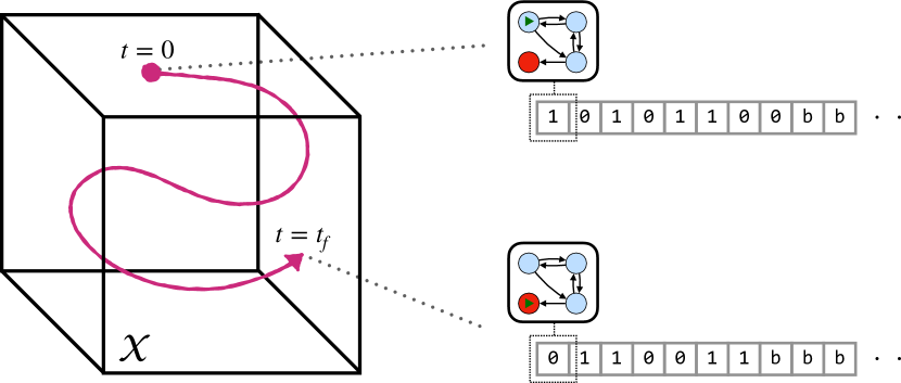
Figure 2: A realization of a TM is a physical process over a countable state space $\mathcal{X}\subseteq{\{0,1\}}^{*}$, which maps initial states to final states according to the input-output function of the TM. As a hypothetical example, consider a process that evolves to the final state 0110011 at $t=t_{f}$ when started on initial state 10101100 at $t=0$ (left), as might correspond to a computation performed by the TM (right, see also Fig. 1).

We briefly describe how a physical process can realize a TM $M$. Without loss of generality, we assume that the countable state space of the physical system $\mathcal{X}$ can be represented by a set of binary strings, so $\mathcal{X}\subseteq{\{0,1\}}^{*}$.

As described in Section II.1 and Appendix A, the computation performed by a TM can be formalized as a partial function $\phi_{M}:{\{0,1\}}^{*}\to{\{0,1\}}^{*}$. We say that a physical process is a realization of a TM $M$ if it realizes the partial function $\phi_{M}$, in the sense of Eq. 13 and 1. Note that this is only possible when $\mathrm{dom\,}\phi_{M}\cup\mathrm{img\,}\phi_{M}\subseteq\mathcal{X}$. Note also that there may be physical states $x\in\mathcal{X}$ that do not belong to $\mathrm{dom\,}\phi_{M}$. When the system is initialized with such states at $t=0$, its will undergo some well-defined dynamical evolution. However, its behavior for such initial states is not constrained by the fact that the system is a realization of the TM, and can be arbitrary (in general, the dynamic and thermodynamic properties for such initial $x$ are not our focus). The mapping between a TM and a physical system is illustrated in Fig. 2.

Many TMs, including all UTMs, can have arbitrarily long programs (i.e., unbounded input length), and can take an arbitrary number of steps before halting on any particular input (i.e., unbounded runtime). For such TMs, our formulation appears to assume a physical system that can store a tape of unbounded size, and which can complete an unbounded number of computational steps in a finite time interval $[0,t_{f}]$, which is not realistic from a physical point of view. In such cases, one can imagine a sequence of realizations, each of which involves manipulating a finite (but growing) tape over a finite (but growing) number of computational steps. Our analysis and results then apply to limit of this sequence, in which the tape size and runtime can be arbitrarily large.

In the following sections, we apply 1 with $f=\phi_{M}$ to establish constraints on the heat function $Q$ of any realization of $M$. We emphasize that in general these constraints do not fully determine the heat function of any realization of $M$: there can be many different realizations of any given TM $M$, each with different heat functions and therefore with different thermodynamic properties (see also wolpert_thermo_comp_review_2019 ). In the next sections, we analyze the thermodynamics of two particular realizations of a given TM, which we call the coin-flipping realization and the dominating realization. We work “backwards” for each one, first specifying its heat function, then using Proposition 1 to establish that there is in fact a realization with that heat function, and then analyzing the properties of that heat function.

Before proceeding, we discuss an important issue concerning the computability properties of realizations of TMs. We say that a realization of a TM $M$ with heat function $Q$ is a computable realization if the function $Q(x)/kT$ is computable (i.e., if there exists a TM that can take as input any $x\in\mathrm{dom\,}\phi_{M}$ and output the value of $Q(x)/kT$ to arbitrary precision). Some of our results below will rely on particular properties of computable realizations. At the same time, some of the realizations we construct and analyze below will not be computable. Whether such non-computable realizations can actually be constructed in the real-world depends on the status of the physical Church-Turing thesis. To see why, imagine that one could construct a non-computable realization of a TM; for example, it might have $Q(x)/kT=K(x)$, where $K(x)$ is the (non-computable) Kolmogorov complexity function. In that case, one could run the realization on various inputs $x$, use a calorimeter to measure the generated heat in units of $kT$ (i.e., measure $Q(x)/kT$), and then arrive at the value of $K(x)$. The above procedure would use a physical process to evaluate a non-computable function, thereby violating the physical Church-Turing thesis.

In this paper, we do not take a position on the validity of the physical Church-Turing thesis. Rather, we will explicitly discuss relevant (non-)computability properties of our realizations, as well as how our non-computable realization can be interpreted in light of the physical Church-Turing thesis. It is important to emphasize, however, that even our non-computable realizations are consistent with the laws of thermodynamics, and are well-defined in terms of a sequence of time-varying Hamiltonians and stochastic dynamics (see the construction in the proof of 1, Appendix C). Their non-computability arises from the fact that our construction uses various idealizations, such as the ability to apply arbitrary Hamiltonians to the system, which are standard in theoretical statistical physics but which disregard possible computational constraints on the set of achievable processes. For example, our construction disregards the fact that, if the physical Church-Turing thesis holds, then it should be impossible to apply non-computable Hamiltonians to the system, such as $H(x)=K(x)$.

IV coin-flipping realization

We first consider a realization of a TM $M$ that achieves zero EP (i.e., is thermodynamically reversible) when run on input programs randomly sampled from a particular input distribution.

To begin, consider the following coin-flipping distribution over programs, which plays an important role in AIT:

$$m_{X}(x):=\begin{cases}2^{-\ell(x)}&\text{if $x\in\mathrm{dom\,}\phi_{M}$}\\ 0&\text{otherwise}\,.\end{cases}$$ (17)

Note that $m_{X}$ sums to a value less than $1$ livi08 , therefore $m_{X}$ is a non-normalized probability distribution. Nonetheless, we refer to it as a “distribution”, following the convention in the AIT literature.

To understand $m_{X}$ more concretely, imagine that the initial state of the TM’s tape is set to a sample of an infinitely long sequence of independent and uniformly distributed bits. Then, $m_{X}(x)$ is proportional to the probability that $M$ eventually halts after reading the bit string $x$ from the tape. Under this hypothetical initialization procedure, the TM will halt on output $y$ with probability

$$m_{Y}(y)=\sum_{{x:\phi_{M}(x)=y}}2^{-\ell(x)}.$$ (18)

This output distribution is biased toward strings that can be generated by short input programs. Note that, like $m_{X}$, this output distribution is not normalized.

We now consider the thermodynamic cost of running a TM on the coin-flipping distribution. We first define a normalized version of the coin-flipping distribution,

$$p_{X}^{\mathrm{coin}}(x):=m_{X}(x)/\Omega_{M},$$ (19)

where $\Omega_{M}:=\sum_{x\in\mathrm{dom\,}\phi_{M}}2^{-\ell(x)}\leq 1$ is a normalization constant (which in AIT is called the “halting probability”). $p_{X}^{\mathrm{coin}}(x)$ is the probability that a TM halts after running input program $x$, conditioned on the TM halting on some input program, given the random initial tape described above. We also define a normalized version of the output distribution,

$$p_{Y}^{\mathrm{coin}}(\phi_{M}(x)):=m_{Y}(\phi_{M}(x))/\Omega_{M}.$$ (20)

Now consider the associated function

$$G(x) =-\ln p_{X}^{\mathrm{coin}}(x)+\ln p_{Y}^{\mathrm{coin}}(\phi_{M}(x)).$$ (21)

It can be verified that this function satisfies condition 2 of 1. Thus, there is at least one realization of $M$, which we call the coin-flipping realization, whose heat function obeys

$$Q_{\mathrm{coin}}(x)=kT\,[-\ln p_{X}^{\mathrm{coin}}(x)+\ln p_{Y}^{\mathrm{coin}}(\phi_{M}(x))].$$ (22)

By plugging $Q_{\mathrm{coin}}$ into Eq. 12, we can verify that this realization achieves $\Sigma(p_{X}^{\mathrm{coin}})=0$, meaning that it is thermodynamically reversible when run on input distribution $p_{X}^{\mathrm{coin}}$.

Eq. 22 can be further simplified by using the definitions of $p_{X}^{\mathrm{coin}}$ and $p_{Y}^{\mathrm{coin}}$:

$$Q_{\mathrm{coin}}(x)=kT\ln 2\,[\ell(x)+\log_{2}m_{Y}(\phi_{M}(x))]\,.$$ (23)

This establishes the claim in the introduction, that the heat generated under the coin-flipping realization on input $x$ is proportional to the length of $x$, minus a “correction term” $-\log_{2}m_{Y}(\phi_{M}(x))$. This correction term is always positive, since $m_{Y}(y)\leq 1$ for all $y$. Moreover, it reflects the logical irreversibility of the partial function $\phi_{M}$ on input $x$: it achieves its minimal value of $-\log_{2}\Omega$ when $\phi_{M}$ maps all inputs to a single output, and its maximal value of $\ell(x)$ when $\phi_{M}$ is logically reversible on input $x$ (i.e., when $x$ is the only input that produces output $\phi_{M}(x)$). In the latter logically reversible case, $Q_{\mathrm{coin}}(x)=0$ for all $x$.

Eq. 23 implies that if one wishes to produce some desired output $y\in\mathrm{img\,}\phi_{M}$ while minimizing heat generation, one should choose the shortest input $x$ such that $\phi_{M}(x)=y$. Loosely speaking, the “less efficient” one is in choosing what program to use to compute $y$, the greater the heat that is expended in that computation. Note that this relationship between shorter programs and less heat generation is not a universal feature of all realizations of TMs. It holds for the coin-flipping realization because this realization is explicitly designed to be thermodynamically-reversible for the coin-flipping input distribution, which has a “built-in bias” for shorter input strings.

An important special case is when the TM of interest is a universal TM. For any UTM $U$, the output distribution in Eq. 18 is called the universal distribution in AIT. The universal distribution possesses many important mathematical properties and is one of the cornerstones of AIT livi08 ; chaitin2004algorithmic ; chai66 ; hutter2008algorithmic ; hutter2003existence , and has attracted attention in artificial intelligence hutter2004universal ; rathmanner2011philosophical ; solo64 ; rissanen1983universal ; hutter2003existence ; schmidhuber2007new , foundations of physics schmidhuber2000algorithmic ; mueller2017law , and statistical physics tadaki_generalization_2002 ; calude_natural_2006 ; tadaki_statistical_2010 ; baez2012algorithmic . In particular, “Levin’s Coding Theorem” livi08 relates the universal distribution to Kolmogorov complexity,

$$-\log_{2}m_{Y}(y)=K(y)+O(1)\,.$$ (24)

This implies that for a UTM, the “correction term” mentioned above is equal to the Kolmogorov complexity of the output, up to an additive constant.

Plugging Eq. 24 into Eq. 23 lets us write the heat function of the coin-flipping realization of a UTM as

$$Q_{\mathrm{coin}}(x)=kT\ln 2\,[\ell(x)-K(\phi_{U}(x))]+O(1)\,.$$ (25)

So for a coin-flipping realization of a UTM, the heat generated on input $x$ reflects how much the length of $x$ exceeds the shortest program which produces the same output as $x$.

These results allow us to calculate the thermodynamic complexity of any output string $y$ using the coin-flipping realization of a UTM $U$, i.e., the minimal heat necessary to generate some desired output $y$:

$$\min_{{x:\phi_{U}(x)=y}}Q_{\mathrm{coin}}(x) =O(1),$$ (26)

where we’ve used Eq. 25 and the fact that $\min_{x:\phi_{U}(x)=y}\ell(x)=K(y)$ by definition. Thus, for the coin-flipping realization, the minimal heat required by the UTM to compute $y$ is bounded by a constant. As emphasized above, this is a fundamental difference between thermodynamic complexity of the coin-flipping realization and Kolmogorov complexity, which is unbounded as one varies over $y$.

However, in order to actually produce a desired output $y$ on a UTM $U$ while generating the minimal possible amount of heat, one needs to know the shortest program for that $y$. Unfortunately, the shortest program for a given output is not computable in general. In fact, we prove in Appendix D that there cannot exist a computable function that maps any desired output $y$ to some corresponding input $x$ such that both $\phi_{U}(x)=y$ and the heat is bounded by a constant, $Q_{\mathrm{coin}}(x)=O(1)$.

We finish by considering the expected heat that would be generated by a realization of a UTM $U$ if inputs were drawn from the distribution $p_{X}^{\mathrm{coin}}$. To begin, rewrite Eq. 12 as

$$\langle Q\rangle_{p_{X}^{\mathrm{coin}}}=kT\,[S(p_{X}^{\mathrm{coin}})-S(p_{Y}^{\mathrm{coin}})+\Sigma(p_{X}^{\mathrm{coin}})]$$ (27)

In Appendix F, we show that the difference of entropies on the RHS of Eq. 27 is infinite. Since $\Sigma(p_{X}^{\mathrm{coin}})$ is always non-negative, any realization of $U$ must, on average, expend an infinite amount of heat to run input programs sampled from $p_{X}^{\mathrm{coin}}$. This applies to the coin-flipping distribution, for which $\Sigma(p_{X}^{\mathrm{coin}})=0$, as well as any other realization. Note that $\ell(x)\geq Q_{\mathrm{coin}}(x)/(kT\ln 2)$ (by Eq. 23 and the fact that $m_{Y}(y)\leq 1$ for all $y$), and that $\ell(x)$ is a lower bound on the number of steps that a prefix UTM needs to run program $x$ (since it must take at least one step per read-in bit). Thus, the fact that programs sampled from the coin-flipping distribution have infinite expected heat generation also implies that they have an infinite expected length, and take an infinite expected number of steps before halting.

We finish by emphasizing that EP and expected heat vary in different ways as one changes the initial distribution. For example, if we run the coin-flipping realization on input distribution $p_{X}^{\mathrm{coin}}$, then EP is zero while expected heat is infinite. On the other hand, since expected heat is a linear function of the input distribution, minimal expected heat corresponds to a delta-function input distribution centered on the $x$ that minimizes $Q_{\mathrm{coin}}(x)$. However, some simple algebra shows that any such delta-function distribution incurs a strictly positive EP for any UTM. Thus, the distribution that minimizes expected heat cannot be the one that minimizes EP.

V Dominating realization

V.1 Minimal possible heat function

We now consider a realization of a TM whose heat function is smaller, up to an additive constant, than the function of any computable realization.

To begin, given any (universal or non-universal) TM $M$, consider the associated function $G(x)=\ln 2\cdot K(x|\phi_{M}(x))$. Note that this conditional Kolmogorov complexity can be defined in terms of any desired UTM, with no a priori relation to $M$. In Appendix E, we show that this function $G$ satisfies condition 2 in 1. Therefore, there must be at least one realization of $M$, which we call the dominating realization, whose heat function obeys

$$Q_{\mathrm{dom}}(x)=kT\ln 2\cdot K(x|\phi_{M}(x)).$$ (28)

Intuitively speaking, the inputs $x$ that generate a large amount of heat under the dominating realization of a TM $M$ are long and incompressible, even when given knowledge of their associated outputs $\phi_{M}(x)$. An example of such an input is a program $x$ that instructs $M$ to read through a long and incompressible bit string and then output nothing, so that $\phi_{M}(x)$ is an empty string (this example is analyzed in more depth below, in Section VI). In contrast, the inputs $x$ that generate little heat under the dominating realization are those in which the output provides a large amount of information about the associated input program. For instance, if $M$ is universal, then a program $x$ that consists of the instruction $\text{``}\texttt{print `}y\texttt{`}\text{''}$ (represented in some appropriate binary encoding) generates little heat, since $K(\text{``}\texttt{print `}y\texttt{`}\text{''}|y)=O(1)$ for any $y$. More generally, if $\phi_{M}$ is logically reversible over its domain, then $K(x|\phi_{M}(x))=O(1)$ for all $x$ in that domain, because one can always reconstruct the input $x$ from the output $\phi_{M}(x)$ by applying $\phi_{M}^{-1}$. Thus, in the (logically reversible) case, the heat generated by the dominating realization on any input $x$ is bounded by a constant that doesn’t depend on $x$.

Now consider any alternative computable realization of $M$ that is coupled to a heat bath at temperature $T$, whose heat function we indicate by $Q$. The assumption of computability means that the function $Q(x)/{kT}$ is computable (i.e., there is some TM that, for any desired $x$, can approximate the value of $Q(x)$ in units of $kT$ to arbitrary precision). As we prove in Appendix E, the heat function of this alternative realization must obey the following inequality,

$$Q(x)\geq Q_{\mathrm{dom}}(x)-kT\ln 2\cdot K(Q/{kT})+K(\phi_{M})+O(1),$$ (29)

where $K(Q/{kT})$ is the Kolmogorov complexity of the heat function $Q$ in units of $kT$, $K(\phi_{M})$ is the Kolmogorov complexity of the partial function computed by $M$, and $O(1)$ represents equality up to an additive constant (that does not depend on $x$, $Q$, or $M$).

Since neither $K(Q/{kT})$ nor $K(\phi_{M})$ depends on the input $x$, Eq. 29 implies $Q(x)\geq Q_{\mathrm{dom}}(x)+\kappa$ for some constant $\kappa$ that is independent of $x$. Note though that $\kappa$ can depend on $\phi_{M}$ (the partial function being computed) and the alternative realization $Q$, and note also that in principle this constant may be arbitrarily large and negative. This means that for any fixed input $x$, there may be computable realizations that result in far less heat when run on $x$ than does the dominating realization. However, this can only occur if $\phi_{M}$ has high complexity (large value of $K(\phi_{M})$), or if the heat function has high complexity, as reflected by a large value of $K(Q/{kT})$. This shows that any computable realization must face a fundamental tradeoff between three different factors: the “lost” algorithmic information about the input in the output, the complexity of the input-output map being realized, and the complexity of the heat function. We explore this tradeoff using an example of erasing a long string in Section VI.

When the TM under question is universal, then it is guaranteed that there exists some program that can generate any desired output $y$. This permits us to analyze the thermodynamic complexity of the dominating realization. It turns out that, as for the coin-flipping realization, this amount is bounded by a constant:

$$\min_{x:\phi_{U}(x)=y}Q_{\mathrm{dom}}(x)=O(1)\,.$$ (30)

This minimum is achieved by programs of the form $x=\text{``}\texttt{print `}y\texttt{`}\text{''}$, since these programs achieve $K(x|\phi_{U}(x))=O(1)$. Eq. 30 also holds if the TM is not a UTM, as long as for each each output $y$, there is some $x$ that obeys $\phi_{M}(x)=y$ and $K(x|\phi_{M}(x))=O(1)$ (e.g., if $\phi_{M}$ is logically reversible).

Finally, we consider the expected heat that would be generated by running the dominating realization of a UTM $U$, assuming that inputs are sampled randomly from some input distribution. To parallel the analysis of the coin-flipping realization, we consider the input distribution which results in minimal EP for the dominating realization, which we call $p_{X}^{*}$. In Appendix F, we prove that the expected heat generated by the dominating realization on the input distribution $p_{X}^{*}$ is infinite. It is interesting to note that $\ell(x)\geq Q_{\mathrm{dom}}(x)/(kT\ln 2)+O(1)$ and, as we mentioned above, $\ell(x)$ is a lower bound on the number of steps that a UTM needs to run program $x$. Thus, the fact that programs sampled from $p_{X}^{*}$ have infinite expected heat generation also implies that they have an infinite expected length, and an infinite expected runtime. Note that the dominating realization of a UTM will in general incur a strictly positive amount of EP, even when run on the optimal input distribution $p_{X}^{*}$ (see Appendix G for details).

V.2 Practical implications of the dominating realization

Our analysis of the dominating realization uses several abstract computer science concepts, such as the computability of the heat function and its Kolmogorov complexity. It is worth making some comments about the real-world significance of such concepts for the thermodynamics of physical systems.

First, the computability properties of the heat function are entirely separate from the computability properties of the logical map $\phi_{M}$ realized by a physical process. In particular, the heat function can be uncomputable even though $\phi_{M}$ is computable by definition (since $\phi_{M}$ is the partial function implemented by a TM). On the other hand, common interpretations of the physical Church-Turing thesis imply that the heat function of any actually constructable real-world physical process must be computable. This implies that, if the physical Church-Turing holds, the dominating realization generates less heat, up to an additive constant, than any realization that can actually be constructed in the real-world.

At the same time, while the dominating realization is better than any computable realization, it is important to note that it itself is not computable. This is because the conditional Kolmogorov complexity is not a computable function, i.e., there is no TM that can take as input two strings $x$ and $y$ and output the value of $K(x|y)$. However, this does not necessarily imply that the dominating realization is irrelevant from a practical point of view. This is because $K(x|y)$ is an upper-semicomputable function, meaning that it is possible to compute an improving sequence of upper bounds that converges on $K(x|y)$. Formally, there is a computable function $f$ such that $f(x,y,n)\geq f(x,y,n+1)$ and $\lim_{n\to\infty}f(x,y,n)=K(x|y)$.

The upper-semicomputability of $Q_{\mathrm{dom}}$ allows one to approach the performance of $Q_{\mathrm{dom}}$ by constructing a sequence $i=1,2,\dots$ of realizations of $\phi_{M}$, each with a computable heat function $Q_{i}$, such that $Q_{i}$ converge from above on $Q_{\mathrm{dom}}$. Each subsequent realization in this sequence is guaranteed to be better (generate less heat) on every input than the previous. Moreover, because the heat functions converge on $Q_{\mathrm{dom}}$, by advancing far enough in this sequence one can run any input $x$ with only $Q_{\mathrm{dom}}+\epsilon$ heat for any $\epsilon>0$. An important subtlety, however, is that one cannot compute how far into the sequence to advance so as to be within $\epsilon$ of $Q_{\mathrm{dom}}$ (if one could compute this, then $Q_{\mathrm{dom}}$ would be computable, and not just upper-semicomputable).

Finally, while we showed that $Q_{\mathrm{dom}}$ is better than any computable realization in terms of heat generation, we also mentioned that it itself is only upper-semicomputable, not computable. One might ask if there is some other upper-semicomputable realization (i.e., one whose heat function can be approached by above) which is even better than $Q_{\mathrm{dom}}$. It is known that this is not the case: the optimality result of Eq. 29 holds not only for any computable $Q$, but more generally for any upper-semicomputable $Q$.

V.3 Comparison of coin-flipping and dominating realizations

We finish our discussion of the dominating realization by briefly comparing it to the coin-flipping realization.

First, for both dominating and coin-flipping realizations, the minimal heat necessary to generate a given output $y$ on a UTM $U$, which we call the thermodynamic complexity of the realization, is bounded by a constant that does not depend on $y$. There is no a priori relationship between those two constants, and in principle it is possible that, for all $y$, the thermodynamic complexity is larger under the dominating realization than the coin-flipping realization, or vice versa. In general, the constants will depend on the realized UTM $U$, as well as the UTM used to define the conditional Kolmogorov complexity in Eq. 28 (which does not have to be the same as $U$).

Second, to achieve bounded heat production for output $y$ under the coin-flipping realization, one must know the shortest program for producing $y$, which is uncomputable. In contrast, to achieve bounded heat production for output $y$ under the dominating realization, it is sufficient to choose an input of the form $\text{``}\texttt{print `}y\texttt{`}\text{''}$.

Third, for both realizations, there is an infinite amount of expected heat generated, assuming that inputs are sampled from the EP-minimizing distribution.

Fourth, the coin-flipping realization is (by design) thermodynamically-reversible for input distribution $p_{X}^{\mathrm{coin}}$. The dominating realization, on the other hand, is not thermodynamically-reversible for any input distribution (see Appendix G).

Finally, neither the coin-flipping nor the dominating realization of a UTM has a computable heat function. In fact, the heat function of the coin-flipping realization is not even upper-semicomputable. This means that our results concerning the superiority of the dominating realization do not apply when comparing to the coin-flipping realization, and in particular it is not necessarily the case that $Q_{\mathrm{coin}}(x)\geq Q_{\mathrm{dom}}(x)+O(1)$. Nonetheless, it turns out that for any UTM $U$, the additional heat incurred by the dominating realization on input $x$, beyond that incurred by the coin-flipping realization, is bound by a logarithmic term in the complexity of the output,

$$Q_{\mathrm{coin}}(x)\geq Q_{\mathrm{dom}}(x)-O(\log K(\phi_{U}(x))).$$ (31)

(See Appendix H for proof.) Such logarithmic correction terms are considered inconsequential in some previous analyses of the thermodynamics of TMs zure89a ; bennett1993thermodynamics .

VI Heat vs. complexity tradeoff

Our analysis of the dominating realization uncovered a tradeoff between heat and complexity faced by any computable physical process. In this section, we illustrate this tradeoff by analyzing the thermodynamics of erasing a long bit string.

As before, consider a physical system with a countable state space, which undergoes driving while coupled to a heat bath at temperature $T$. For notational simplicity, in this section we choose units so that $kT=1$. Assume that the process realizes some deterministic and computable map from initial to final states, which we indicate generically as $f:{\{0,1\}}^{*}\to{\{0,1\}}^{*}$. Now imagine that one observes a single realization of this physical process, in which initial state $x$ is mapped to final state $y=f(x)$.

Since this is a computable realization of $f$, it must obey the dominating realization bound of Eq. 29. Plugging Eq. 28 into that inequality and rearranging gives

$$Q(x)/\ln 2+K(Q)+K(f)\geq K(x|y)+O(1),$$ (32)

where we’ve used the assumption that $kT=1$. This shows that there is a fundamental cost of $K(x|y)$ that is incurred by any computable realization that maps input $x$ to output $y$. This fundamental cost can be paid either by generating a lot of heat (large $Q(x)/\ln 2$), by having a high complexity heat function (large $K(Q)$), or by realizing a high-complexity input-output function (large $K(f)$). This tradeoff is illustrated in Fig. 3.

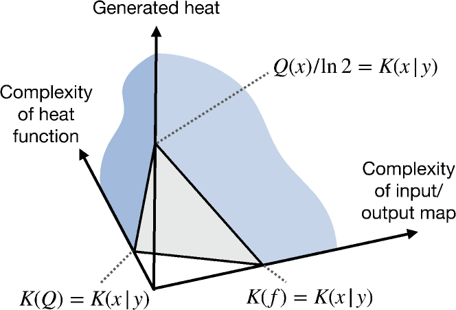
Figure 3: Any computable process that realizes a deterministic input-output map $f$ faces a fundamental cost of $K(x|y)$ for mapping input $x$ to output $y=f(x)$. This cost can be paid through some combination of three different strategies: generating a large amount of heat, having a high complexity heat function, or having a high complexity input-output map $f$. This tradeoff is illustrated on three axes, with blue indicating the feasible region.

We demonstrate this tradeoff using an example of a process that erases a long binary string. In this example, $x$ is a long string consisting of $n$ binary digits, while the final state $y$ is a string of $n$ 0s, which we write ‘00...00’. Assuming $x$ is incompressible (which is true for the vast majority of all strings), the fundamental cost of mapping $x\to y$ is given by $K(x|y)=K(x)\approx\ell(x)$ up to logarithmic factors livi08 . Different processes can pay this fundamental cost in different ways, thereby satisfying Eq. 32:

(1) A process can generate a lot of heat. For example, in order to erase string $x$, the process can run an erasure map:

$$f(x^{\prime}):={\small\text{`{00...00}'}}\qquad\forall x^{\prime},$$ (33)

while using the dominating implementation. In this case, $Q(x)/\ln 2=K(x|y)$ by Eq. 28.

(2) A process can have a high-complexity heat function, so that $K(Q)\geq\ell(x)$. For example, one can tweak the dominating realization of the erasure map, so that the heat values for input $x$ and the input consisting of all 0s are swapped:

$$Q(x^{\prime}):=\begin{cases}Q_{\mathrm{dom}}(x^{\prime})&\text{if $x^{\prime}\not\in\{x,{\small\text{`{00...00}'}}\}$}\\ Q_{\mathrm{dom}}({\small\text{`{00...00}'}})&\text{if $x^{\prime}=x$}\\ Q_{\mathrm{dom}}(x)&\text{if $x^{\prime}={\small\text{`{00...00}'}}$}\end{cases}$$

One can verify that since $Q_{\mathrm{dom}}$ satisfies condition 2 in 1, so does this $Q$. Moreover, this realization generates a small amount of heat when erasing $x$,

$$Q(x) =Q_{\mathrm{dom}}({\small\text{`{00...00}'}})$$

$$=K({\small\text{`{00...00}'}}|{\small\text{`{00...00}'}})\approx 0.$$

Note, however, that the long input string $x$ is now “hard-coded” into the definition of the heat function $Q$, leading to a large value of $K(Q)$.

(3) A process can realize a high-complexity input-output map $f$, so that $K(f)\geq K(x|y)$. This strategy could be used, for example, by a process which implements the following logically reversible map:

$$f(x^{\prime}):=\begin{cases}x^{\prime}&\text{if $x^{\prime}\not\in\{x,{\small\text{`{00...00}'}}\}$}\\ {\small\text{`{00...00}'}}&\text{if $x^{\prime}=x$}\\ x&\text{if $x^{\prime}={\small\text{`{00...00}'}}$}\end{cases}$$

Since logically reversible function can be carried out without generating heat, it is possible to implement this $f$ while achieving $Q(x^{\prime})=0$ for all $x^{\prime}$. In this case, not only does erasing $x$ not generate any heat, $Q(x)=0$, but the heat function has low complexity, $K(Q)\approx 0$. Now, however, the long input string $x$ is “hard-coded” into the definition of the input-output map $f$, leading to a large value of $K(f)$.

We finish by noting that in a series of papers by Zurek and others zure89a ; zure89b ; bennett1993thermodynamics ; bennett1998information ; baumeler2019free ; li1992mathematical ; caves1990entropy ; caves1993information ; zurek1990algorithmic , it was argued that the conditional Kolmogorov complexity $K(x|y)$ is “the minimal thermodynamic cost” of computing some output $y$ from input $x$. However, most of these early papers were written before the development of modern nonequilibrium statistical physics. As a result, the arguments in those papers are rather informal, which in turn makes it difficult to translate them in a fully rigorous manner into modern nonequilibrium statistical physics. (See Sec. 14.4 in wolpert_thermo_comp_review_2019 for one possible translation.) To give one example of these difficulties, those earlier analyses quantified the “thermodynamic cost” in terms of the number of physical bits (binary degrees of freedom) that are erased during that computation, independent of the initial probability distributions over those binary degrees of freedom. However, we now know that minimal heat generation is given by changes in Shannon entropy, i.e., in terms of statistical bits rather than physical bits. Relatedly, these papers led to some proposals that the foundations of statistical physics be changed, so that thermodynamic entropy is identified not only with Shannon entropy, but also a Kolmogorov complexity term zure89b ; livi08 .

In contrast, our analysis is grounded in modern nonequilibrium physics, and does not involve any foundational modifications to the definition of thermodynamic entropy. Moreover, it covers some issues not considered in earlier analyses. In particular, we show that the lower bound of $K(x|y)$ is a cost that in general applies only to computable realizations (i.e., ones with a computable heat function), not for all possible realizations, as implied in the earlier papers. The significance of this restriction depends on the legitimacy of the physical Church-Turing thesis. Finally, we also demonstrate different ways in which one can pay the fundamental cost $K(x|y)$: by either generating heat, by having a large Kolmogorov complexity of the heat function $K({Q})$, or by having a large Kolmogorov complexity of the input-output map, $K(f)$.

VII Discussion

In this paper we combine Algorithmic Information Theory (AIT) and nonequilibrium statistical physics to analyze the thermodynamics of TMs. We consider a physical process that realizes a deterministic input-output function, representing the computation performed by some TM. We derive numerous results concerning two different realizations of TM: a coin-flipping realization, which is designed to be thermodynamically reversible when fed with random input bits, and a dominating realization, which is designed to generate less heat than any computable realization.

Using our analysis of the dominating realization, we uncover a fundamental tradeoff, faced by any computable realization of a deterministic input-output map, between heat generation, the Kolmogorov complexity of the heat function, and the Kolmogorov complexity of the input-output map. An interesting topic for future research is how the Kolmogorov complexity of the heat function and the input-output map relates to the “physical complexity” of the driving process, as commonly understood in physics (e.g., whether the Hamiltonians must have many-body interactions, etc.).

For simplicity, in this paper we represented a TM $M$ as a physical system whose dynamics carries out the partial function $\phi_{M}:{\{0,1\}}^{*}\to{\{0,1\}}^{*}$ during some finite time interval $[0,t_{f}]$. This representation allowed us to abstract away many implementation details of the realization, such as the fact that a TM consists of a separate tape, head, and pointer variables, and that a TM operates in a sequence of discrete steps. Essentially, this representation does not distinguish whether the physical process operates via the same sequence of steps as a TM, or simply implements a “lookup table” that maps outputs to inputs.

While this representation simplifies our analysis, it provides no guidance on how to actually construct a physical process that realizes a TM in the laboratory, and it leaves implicit some important issues. Alternatively, one could represent a realization of a TM in a more conventional and “mechanistic” way, as a dynamical system over the state of the TM’s tape, pointer, and head, which evolves iteratively according to the update function of the TM until the head reaches the halt state. In contrast to the representation we adopted, this kind of mechanistic representation could easily be physically constructed, and would correspond more closely to the step-by-step operation of real-world physical computers. Moreover, this kind of mechanistic representation could be used to analyze the thermodynamic costs of TMs in a more realistic manner. For example, it could be used to analyze how the heat and EP incurred by the TM depends on the number of steps taken. As another example, it could be used to impose constraints on how the degrees of freedom of the head, tape, and pointer can be coupled together (e.g., via interaction terms of applied Hamiltonians). One might postulate, for instance, that the head of the TM can only interact with tape locations that are located near the pointer. These kinds of constraint will generally increase the heat and EP incurred by each step of the TM wolpert_thermo_comp_review_2019 ; circuits2020 . These complications concerning the thermodynamics of more mechanistic representations of TMs are absent from the analysis in this paper, and are topics of future research.

Appendix A Models of single-tape TMs

In this appendix we present a formal definition of a single-tape TM.

In Section II.1, we define the state of a TM as being composed of a tape state $s\in A^{\infty}$, a pointer state $v\in\mathbb{N}$, and head state $h\in H$. Here, $A$ is a finite alphabet of tape symbols which includes a special “blank” symbol, while $H$ is a finite set of head states which includes a special “start” head state and a special “halt” head state. Any particular value of the triple $(s,v,h)$ is called an instantaneous description (ID) of the TM. The dynamics of a particular TM is given by iteratively applying an update function $f$ to the ID,

$$f:(s,v,h)\mapsto(s^{\prime},v^{\prime},h^{\prime})\,.$$ (34)

Following standard definitions, we assume that $f(s,v,h)$ only depends on $(s(v),h)$, i.e., the next ID of the TM can only depend on the current state of the head and the current contents of the tape $s$ at position $v$. We also assume that the new value of the pointer $v^{\prime}$ does not differ by more than $1$ from $v$, and that the tape state $s^{\prime}$ be identical to the tape state $s$ at all positions, except possibly position $v$. By iteratively applying $f$, the head moves back and forth along the tape, while both changing its state as well as reading and writing symbols onto the tape at its current position.

At the beginning of a computation, the state of the TM must be a valid initial ID, meaning that the head $h$ is in the start state, the pointer is set to $v=1$, and the tape $s$ consists of finite string of non-blank symbols, followed by an infinite sequence of blank symbols. The TM then visits a sequence of IDs by iteratively applying the update function $f$. The TM stops if the head ever reaches the halt state (i.e., any ID where the head in the halt state is a fixed point of $f$). In general, there can be valid initial IDs for which the TM never halts.

For simplicity, we assume that $0$ and $1$ are elements of the alphabet $A$, and that the non-blank finite string at the beginning of the initial tape state is some $x\in{\{0,1\}}^{*}$. In addition, we assume that if the head of the TM reaches a halt state after starting from some valid initial ID, then at that time the pointer is set to $1$ and the final tape state begins with some $y\in{\{0,1\}}^{*}$, followed by blank symbols. In that case, we refer to the string $x\in{\{0,1\}}^{*}$ as the input or program for the TM, and the corresponding string $y\in{\{0,1\}}^{*}$ as the output of the TM for program $x$.

Given these assumption, we can represent the overall computation performed by a TM $M$ as a partial function $\phi_{M}:{\{0,1\}}^{*}\to{\{0,1\}}^{*}$. Here, $\phi_{M}(x)=y$ indicates that when the TM is initialized with its tape containing $x$ followed by an infinite sequence of blank symbols, then it will halt with its tape containing $y$ followed by an infinite sequence of blank symbols. If the TM does not halt for some particular initial tape state $x$, then the value of $\phi_{M}(x)$ is undefined (for this reason, in general $\phi_{M}$ is a partial function). When we talk about a realization of a TM $M$ in the main text, we refer to a physical process over a countable state space, whose dynamics from initial states to final states can be mapped onto the partial function $\phi_{M}$ implemented by some TM $M$.

As we mention in the main text, we assume that any TM under consideration is a prefix TM, meaning that it has a prefix-free halting set. Prefix TMs are typically TMs with multiple tapes, where one of the tapes is a read-only input tape that is read left-to-right livi08 . If this kind of multi-tape machine halts after reading some string $x$ from the input tape, it means that the machine did not halt after reading some string $x^{\prime}$ on the input tape which is a strict prefix of $x$ (otherwise, it would never get to read-in all of $x$), thereby guaranteeing the prefix property. For simplicity, however, in this paper we assume that the prefix TM is single-tape. This can be done without loss of generality, as it is always possible to transform a prefix TM with multiple tapes into an equivalent single-tape prefix TM, using any of the conventional techniques for transforming between multi-tape and single-tape TMs (see (papadimitriou2003computational, , Thm. 2.1) and sipser2006introduction for details). Note that these techniques may involve adding additional symbols to the tape alphabet $A$, which may be used at intermediate steps of the computation.

Appendix B Decomposition of entropy production

In this appendix, we derive a useful decomposition of the EP incurred by a realization of a deterministic input-output function. We also relate this decomposition to our previous work, which analyzed the dependence of EP on the initial distribution of a process kolchinsky2016dependence ; wolpert_thermo_comp_review_2019 ; circuits2020 .

Consider some physical process that realizes the function $f:\mathcal{X}\to\mathcal{X}$, in the sense of Eq. 13. Then, the conditional distribution of an initial state $x\in\mathrm{dom\,}f$ given final state $f(x)$ can be written as

$$p_{X|f(X)}(x|f(x)):=\dfrac{p_{X}(x)}{\sum_{x^{\prime}:f(x^{\prime})=f(x)}p_{X}(x^{\prime})}.$$ (35)

We use this expression to rewrite the EP from Eq. 12 as

$$\Sigma(p_{X})=$$ (36)

$$\quad\sum_{x}p_{X}(x)\bigg{[}\ln\frac{p_{X|f(X)}(x|f(x))}{e^{-Q(x)/{kT}-\ln Z(f(X))}}-\ln Z(f(x))\bigg{]},$$

where we have defined

$$Z(y):=\sum_{x:f(x)=y}e^{-{Q(x)}/kT}.$$ (37)

Now, define the following conditional distribution,

$$w_{X|f(X)}(x|f(x)):=e^{-Q(x)/kT}-\ln Z(f(x)).$$ (38)

Using this definition, we can further rewrite Eq. 36 as

$$\Sigma(p_{X}) =D(p_{X|f(X)}\|w_{X|f(X)})-\langle\ln Z(f(x))\rangle_{p_{X}},$$ (39)

where $D(p_{X|f(X)}\|w_{X|f(X)})$ indicates the conditional KL divergence between the conditional distribution $p_{X|f(X)}$ and $w_{X|f(X)}$ cover_elements_2012 .

As we show below in Eq. 40, $-\ln Z(f(x))\geq 0$ for all $x$. Thus, Eq. 39 implies $\Sigma(p_{X})\geq D(p_{X|f(X)}\|w_{X|f(X)})$. Note that this lower bound is non-negative, and vanishes whenever $p_{X|f(X)}=w_{X|f(X)}$. This means that $w_{X|f(X)}$, as defined in Eq. 38, encodes that conditional probability of inputs $x$ given outputs $f(x)$ that achieves minimal EP for a realization of $f$ with heat function $Q$.

In our previous work, we have sometimes referred to the conditional KL divergence in Eq. 39 as mismatch cost. Using the chain rule for KL divergence, we write mismatch cost as

$$D(p_{X|f(X)}\|w_{X|f(X)})=D(p_{X}\|w_{X})-D(p_{f(X)}\|w_{f(X)})\,,$$

where $w_{f(X)}(y)=\sum_{x:f(x)=y}w_{X}(x)$, while $w_{X}(x)$ is any distribution that obeys

$$w_{X}(x)/w_{X}(x^{\prime})=e^{[Q(x^{\prime})-Q(x)]/{kT}}\quad\forall x,x^{\prime}:f(x)=f(x^{\prime}).$$

In our previous, we referred to the distribution $w_{X}(x)$ as a prior. (This term was originally motivated by a Bayesian interpretation of EP kolchinsky2016dependence .) As long as $|\mathrm{img\,}f|>1$, there are an infinite number of priors for any given $w_{X|f(X)}$, since the relative probabilities of any pair $x,x^{\prime}$ with $f(x)\neq f(x^{\prime})$ are unconstrained.

In our previous work wolpert_thermo_comp_review_2019 ; circuits2020 , we referred to the term $-\langle\ln Z(f(X))\rangle_{p_{X}}$ in Eq. 39 as the residual EP. Observe that for any $y\in\mathrm{img\,}f$,

$$\Sigma(w_{X|f(X)=y}) =D(w_{X|f(X)=y}\|w_{X|f(X)})-\ln Z(y)$$

$$=-\ln Z(y).$$ (40)

Since $\Sigma(w_{X|f(X)=y})\geq 0$ by the second law, $-\ln Z(y)$ is non-negative for all $y\in\mathrm{img\,}f$ and therefore residual EP is always non-negative. Note also that the residual EP is an expectation under $p_{X}$, thus it is linear in $p_{X}$. In fact, it only depends on the probabilities assigned to each output $p_{f(X)}(y)$, not the conditional distribution of inputs corresponding to each output. In our other work circuits2020 , we’ve sometimes called the indexed set $\{-\ln Z(y)\}_{y}$ the residual EP parameter.

Finally, define an island of $f$ as a pre-image $f^{-1}(y)$ for some $y$, with $L(f)$ the set of all islands of $U$. We can rewrite Eq. 39 as

$$\Sigma(p_{X})=\sum_{\mathclap{c\in L(f)}}p(c)\left[D\left(p_{X|X\in c}\|w_{X|X\in c}\right)-\ln Z(f(c))\right],$$

where $p(c)=\sum_{x\in c}p_{X}(x)$. Intuitively, this expression shows that any realization of the function $f$ can be thought of a set of (island-indexed) “parallel” processes, operating independently of one another on non-overlapping subsets of $\mathcal{X}$, each generating EP given by the associated mismatch cost and residual EP.

This form of mismatch cost, residual EP, and island decomposition was introduced in kolchinsky2016dependence ; wolpert_thermo_comp_review_2019 ; circuits2020 . It holds even in the general case of non-deterministic dynamics, with an appropriate (more general) definition of the prior $w_{X}$ and the island decomposition. However, that previous work on mismatch cost and residual EP assumed finite state spaces. The derivation presented above does not have that restriction.

Appendix C Proof of 1

The following proof will make use of the decomposition of EP derived in Appendix B.

See 1

Proof.

Note that condition 1 follows from condition 3 by the second law of thermodynamics. To show equivalence of all three conditions, we proceed in the following way:

1. We show that condition 2 is implied by condition 1.

2. We show that condition 1 is implied by condition 2.

3. We show by construction that condition 2 implies condition 3.

Given that $\mathcal{X}$ is countable, we assume that $\mathcal{X}\subseteq\mathbb{N}$. This is done without loss of generality: if elements of $\mathcal{X}$ are not natural numbers, one can put a total order on $\mathcal{X}$ using the natural numbers.

We now prove that condition 1 implies condition 2. First, define the function $F$ to refer the expression in Eq. 14,

$$F(p_{X})=\sum_{x}p_{X}(x)\big{[}G(x)-\ln p_{f(X)}(f(x))+\ln p_{X}(x)\big{]}.$$ (41)

Let $\mathcal{A}_{n}(y)$ indicate the first $n$ elements of $f^{-1}(y)$, and define the initial distribution

$$p_{X}^{(n)}(x)=\begin{cases}e^{-G(x)}/Z_{n}(y)&\text{if $x\in\mathcal{A}_{n}(y)$}\\ 0&\text{otherwise}\end{cases},$$

where $Z_{n}(y)=\sum_{x\in\mathcal{A}_{n}(y)}e^{-G(x)}$. Note that $\operatorname{supp}p_{X}^{(n)}\subseteq\mathrm{dom\,}f$. Plugging into Eq. 41 and simplifying gives

$$F(p_{X}^{(n)})=-\ln Z_{n}(y)\geq 0\,,$$

or equivalently $Z_{n}(y)\leq 1$. Since this holds for all $n$,

$$Z(y) =\sum_{\mathclap{x:f(x)=y}}\;e^{-G(x)}=\lim_{n\rightarrow\infty}Z_{n}(y)\leq 1\,.$$ (42)

We now prove that condition 1 is implied by condition 2. Define $w_{X|f(X)}(x|f(x))$ as in Eq. 38, while taking $Q/{kT}=G$. Then, use the results in Appendix B to rewrite $F$ as

$$F(p_{X}) =D(p_{X|f(X)}\|w_{X|f(X)})-\langle\ln Z(f(X))\rangle_{p_{X}}$$

$$\geq D(p_{X|f(X)}\|w_{X|f(X)})\geq 0.$$

The first inequality follows from the assumption that $Z(y)=\sum_{x:f(x)=y}e^{-G(x)}\leq 1$ for all $y\in\mathrm{img\,}f$, and the second inequality follows from the non-negativity of conditional KL divergence cover_elements_2012 .

The rest of this proof shows by construction that condition 3 follows from condition 2. For simplicity, assume that the physical process has access to a set of “auxiliary” states, one for each $y\in\mathrm{img\,}f$. We use $x_{y}$ to indicate the auxiliary state corresponding to each $y$, and assume that $x_{y}\not\in\mathrm{dom\,}f$. For notational convenience, let ${\mathcal{W}}:=\mathrm{dom\,}f\cup\{x_{y}:y\in\mathrm{img\,}f\}$. Then, define the following function $\hat{f}:{\mathcal{W}}\to\mathcal{X}$,

For any $$x\in\mathrm{dom\,}f \hat{f}(x):=f(x)\,,$$,

For any $$y\in\mathrm{img\,}f \hat{f}(x_{y}):=y\,.$$,

In words, any $x$ in the domain of $f$ is mapped by $\hat{f}$ to $f(x)$, while any auxiliary state $x_{y}$ is mapped by $\hat{f}$ to $y$.

Now, define the following Hamiltonian $H:{\mathcal{W}}\to\mathbb{R}\cup\{\infty\}$,

$$\!\!\!\forall x\in\mathrm{dom\,}f:H(x):=f(x)+kT\,G(x)$$ (43)

$$\!\!\!\forall y\in\mathrm{img\,}f:H(x_{y}):=y-kT\,\ln\left(1-\sum_{\mathclap{x:f(x)=y}}e^{-G(x)}\right).$$ (44)

We use $\pi(w)=e^{-{H(w)}/kT}/Z$ to indicate the Boltzmann distribution for Hamiltonian $H$, where $Z=\sum_{x\in{\mathcal{W}}}e^{-{H(x)}/kT}$ is the partition function. Note that the partition function converges when $\beta>0$,

$$Z =\sum_{y\in\mathrm{img\,}f}\Bigg{[}e^{-{H(x_{y})}/kT}+\sum_{x:f(x)=y}e^{-{H(x)}/kT}\Bigg{]}$$ (45)

$$=\sum_{y\in\mathrm{img\,}f}e^{-{y}/kT}\leq\sum_{i\in\mathbb{N}}e^{-{i}/kT}=1/(e^{1/{kT}}-1).$$

To derive the second line, we plugged Eqs. 43 and 44 into Eq. 45 and simplified.

We now consider the following physical process over $t\in[0,t_{f}]$, applied to a system coupled to a work reservoir and a heat bath at temperature $T$:

1. At $t=0$, the Hamiltonian $H$ is applied to the system.

2. Over $t\in(0,\tau]$, the system is allowed to freely relax toward equilibrium. However, the only allowed transitions are those between pairs of states $w,w^{\prime}$ that have $\hat{f}(w)=\hat{f}(w^{\prime})$. We assume that by $t=\tau$, the system has reached a stationary distribution.

3. Over $t\in(\tau,t_{f}]$, the system undergoes a quasistatic physical process that implements the map $\hat{f}$ from initial to final states, and does so in a thermodynamically reversible way for initial distribution $\pi$. There are numerous known ways of constructing such a process turgut_relations_2009 ; maroney2009generalizing ; wolpert_spacetime_2019 .

Note that the above procedure assumes a separation of timescales (i.e., the relaxation time of the system is infinitely faster than $\tau$ and $t_{f}-\tau$). Step (3) also assumes an idealized heat bath (infinite heat capacity, weak coupling, infinitely fast relaxation time deffner2013information ).

The above procedure will map any $x\in\mathrm{dom\,}f$ to final state $f(x)$. Let $Q$ indicate the heat function of this process. We will show that $Q(x)/{kT}=G(x)$ for any $x\in\mathrm{dom\,}f$. First, let $\delta_{x}$ indicate an initial distribution which is a delta function over some state $x$. Note that

$$\Sigma(\delta_{x}) =S(\delta_{f(x)})-S(\delta_{x})+\langle Q\rangle_{\delta_{x}}/{kT}=Q(x)/{kT},$$ (46)

where we’ve used the fact that $S(\delta_{x})=S(\delta_{f(x)})=0$. We then analyze $\Sigma(\delta_{x})$. Step (1) and step (3) in the above construction incur no EP. For step (2), EP incurred during free relaxation from $t=0$ to $t=\tau$ is given by

$$\Sigma(\delta_{x})=D(\delta_{x}\|\pi)-D(p^{\tau}_{x}\|\pi)\,,$$ (47)

where $p^{\tau}_{x}$ is the state distribution at time $\tau$, given that the system started in distribution $\delta_{x}$ at $t=0$. By construction, $p^{\tau}_{x}$ will be equal to the equilibrium distribution restricted to a subset of states,

$$p^{\tau}_{x}(w)=\frac{\delta(\hat{f}(w),\hat{f}(x))\pi(w)}{\sum_{w^{\prime}}\delta(\hat{f}(w^{\prime}),\hat{f}(x))\pi(w^{\prime})}.$$

It can be verified, using the definition of $\delta_{x}$ and $\pi$, that

$$D(\delta_{x}\|\pi)=f(x)/{kT}+G(x)+\ln Z.$$

Similarly, it can be verified using the definition of $p^{\tau}_{x}$ that

$$D(p^{\tau}_{x}\|\pi) =f(x)/{kT}+\ln Z.$$

Plugging these two KL divergences into Eq. 47 gives

$$\Sigma(\delta_{x})=G(x).$$ (48)

Combining with Eq. 46 gives $Q(x)/{kT}=\Sigma(\delta_{x})=G(x)$.

∎

It can be verified that the physical process constructed in the proof of 1 is thermodynamically reversible if it is started with the initial equilibrium distribution $\pi_{X}$, so that the free relaxation in step 2 incurs no EP. Generally, this equilibrium distribution will have support on the auxiliary states, which are outside of $\mathrm{dom\,}f$. However, consider the case when Eq. 15 is an equality for all $y\in\mathrm{img\,}f$. Then, the definition in Eq. 44 gives $H(x_{y})=\infty$ and $\pi_{X}(x_{y})=0$ for all $y\in\mathrm{img\,}f$. In this case, the input distribution $p_{X}=\pi_{X}$ obeys $\operatorname{supp}p_{X}\subseteq\mathrm{dom\,}f$ and achieves zero EP. Moreover, using the decomposition in Appendix B, it can be verified that if Eq. 15 is an equality for all $y\in\mathrm{img\,}f$, then any input distribution that obeys $p_{X|f(X)}=\pi_{X|f(X)}$, as defined in Eq. 35, also achieves zero EP.

Appendix D $O(1)$ heat for coin-flipping realization is uncomputable

Let $\phi_{U}$ indicate the partial function computed by some UTM $U$. Imagine there is some computable function $f$ such that for any $y$, $f(y)$ returns an input for $\phi_{U}$ that outputs $y$ and generates bounded heat under the coin-flipping realization (i.e., $\phi_{U}(f(y))=y$ and $Q_{\mathrm{coin}}(f(y))=O(1)$). Then, by Eq. 25, it must be that $\ell(f(y))=K(y)+O(1)$. Since $\ell(\cdot)$ is a computable function, this would in turn imply that there is a computable function $g(y)=K(y)+O(1)$. However, such a function cannot exist, as shown in the following proposition.

Proposition 1.

There is no computable partial function $g:{\{0,1\}}^{*}\to\mathbb{N}$ such that for all $y$,

$$g(y)=K(y)+O(1)\,.$$ (49)

Proof.

We say that $p_{Y}(y)$ is a semimeasure if $p_{Y}(y)\geq 0$ for all $y$ and $\sum_{y}p_{Y}(y)\leq 1$ (i.e., it is a non-normalized probability distribution). We say that a semimeasure $p_{Y}(y)$ (multiplicatively) dominates another semimeasure $q_{Y}(y)$ if there is some constant $c>0$ such that $p_{Y}(y)\geq c\cdot q_{Y}(y)$ for all $y$.

Assume that a computable $g(y)=K(y)+O(1)$ exists. Then, $q_{Y}(y):=2^{-g(y)}$ would be a computable semimeasure that dominates $p_{Y}(y):=2^{-K(y)}$. It is known that $p_{Y}(y)$ dominates every computable semimeasure (livi08, , Thm. 4.3.3 and Cor. 4.3.1). Since domination is transitive, if $g(y)$ were computable then $q_{Y}(y)$ would be a computable semimeasure that dominates every computable semimeasure. However, such a semimeasure cannot exist by Lemma 4.3.1 in livi08 . ∎

Appendix E Proof of Eq. 29

Let $f$ indicate any computable partial function. In this appendix, we show that the dominating realization of $f$, with heat function

$$Q_{\mathrm{dom}}(x)=kT\ln 2\cdot K(x|f(x)),$$ (50)

is better than any other realization of $f$ with an upper-semicomputable heat function $Q$, up to an additive constant.

We first prove the following two useful results.

Lemma 2.

For any partial function $f:{\{0,1\}}^{*}\to{\{0,1\}}^{*}$,

$$\sum_{\mathclap{x:f(x)=y}}e^{-\ln 2\cdot K(x|y)}\leq 1\qquad\forall y\in\mathrm{img\,}f.$$

Proof.

For all $y\in\mathrm{img\,}f$, we have the following:

$$\sum_{\mathclap{x:f(x)=y}}e^{-\ln 2\cdot K(x|y)}=\sum_{\mathclap{x:f(x)=y}}2^{-K(x|y)}\leq\sum_{\mathclap{x\in{\{0,1\}}^{*}}}2^{-K(x|y)}.$$

In addition, we have the bound

$$\sum_{\mathclap{x\in{\{0,1\}}^{*}}}2^{-K(x|y)}\leq 1,$$ (51)

which comes from Kraft’s inequality and the fact that, for any given $y$, the set $\{K(x|y):x\in{\{0,1\}}^{*}\}$ specifies the lengths of a prefix-free code (livi08, , p. 252 and p. 287). Combining gives the desired result.∎

Proposition 3.

Let $f:{\{0,1\}}^{*}\to{\{0,1\}}^{*}$ be a computable partial function, $Q:{\{0,1\}}^{*}\to{\mathbb{R}}$ a upper-semicomputable partial function with $\mathrm{dom\,}Q\supseteq\mathrm{dom\,}f$. If for all $y\in\mathrm{img\,}f$,

$$\sum_{x:f(x)=y}e^{-Q(x)}\leq 1,$$ (52)

then for all $x\in\mathrm{dom\,}f$,

$$Q(x)\geq\ln 2\cdot[K(x|f(x))-K(Q,f)]+O(1)\,,$$ (53)

where $O(1)$ is a constant independent of $x$ and $Q$.

Proof.

Let $M$ indicate the TM that computes $f$, and let $a(x,n)$ be a computable partial function which upper-semicomputes $Q(x)/\ln 2$. Then, define the following TM $B$: given inputs $x\in{\{0,1\}}^{*}$, $y\in{\{0,1\}}^{*}$, and $n\in\mathbb{N}$, the TM $B$ runs $M$ for $n$ steps on input $x$. If $M$ halts within that time on output $y$, then $B$ outputs $2^{-a(x,n)}$. Otherwise, $B$ outputs 0 and halts.

Then, for any $x\in\mathrm{dom\,}f$, define

$$s(x|y) :=\lim_{n\rightarrow\infty}\phi_{B}(\langle x,y\rangle,n)$$

$$=\delta(f(x),y)2^{-Q(x)/\ln 2}$$

$$=\delta(f(x),y)e^{-Q(x)}.$$ (54)

It is easy to check that $\phi_{B}(\langle x,y\rangle,n)$ is non-decreasing in $n$, so $s(x|y)$ is lower-semicomputable (i.e., $\phi_{B}(\langle x,y\rangle,n)\leq\phi_{B}(\langle x,y\rangle,n+1)$ and $\lim_{n\to\infty}\phi_{B}(\langle x,y\rangle,n)=s(x|y)$). Moreover, if one had a program that computed both $f$ and $Q$, then one could lower-semicompute $s$. This means that

$$K(s)\leq K(Q,f)+O(1),$$ (55)

where $K(Q,f)$ is the Kolmogorov complexity of jointly computing the functions $f$ and $Q$.

By assumption in Eq. 52, for any $y\in\mathrm{img\,}f$,

$$\sum_{\mathclap{x\in\mathrm{dom\,}f}}s(x|y)=\sum_{\mathclap{x:f(x)=y}}2^{-Q(x)/\ln 2}=\sum_{\mathclap{x:f(x)=y}}e^{-Q(x)}\leq 1.$$ (56)

This means that $s(x|y)$ is a so-called conditional semimeasure of $x$ given $y$ (i.e., a non-normalized conditional probability measure). For any lower-semicomputable conditional semimeasure $s$, an existing result in AIT (vitanyi2013conditional, , Cor. 2) states

$$K(x|y) \leq-\log_{2}s(x|y)+K(s)+O(1).$$

Taking $y=f(x)$ and plugging in Eqs. 54 and 55 gives

$$K(x|f(x)) \leq Q(x)/\ln 2+K(Q,f)+O(1).$$ (57)

Eq. 53 follows by rearranging. ∎

Given that Eq. 52 holds, by 1 there must be a realization of $f$ with heat function $Q(x)=kTG(x)$. By Lemma 2, we can take $G(x)=\ln 2\cdot K(x|f(x))$. Thus, there must exists a realization of $f$ with heat function $Q_{\mathrm{dom}}$, as defined in Eq. 50.

Combining $G(x)=Q(x)/kT$ with Eq. 53, and multiplying both sides by $kT$, gives the following inequality,

$$Q(x)\geq Q_{\mathrm{dom}}(x)-kT\ln 2\cdot K(Q/{kT},f)+O(1)\,.$$

We can derive a slightly weaker, but more interpretable, lower bound by using $K(Q/{kT},f)\leq K(Q/{kT})+K(f)+O(1)$, which follows from the subadditivity of Kolmogorov complexity (livi08, , p.202). This allows to rewrite the above as

$$Q(x)\geq Q_{\mathrm{dom}}(x)-kT\ln 2\,[K(Q/{kT})+K(f)]+O(1),$$

which appears in the main text as Eq. 29, with $f=\phi_{M}$.

Appendix F Infinite expected heat

Let $\phi_{U}$ be the partial function computed by some UTM $U$. In the following results, we will make use of the following decomposition of the drop of entropy, which holds for any initial distribution $p_{X}$:

$$S(p_{X})-S(p_{Y}) =\sum_{\mathclap{y\in\mathrm{img\,}\phi_{U}}}p_{Y}(y)S(p_{X|\phi_{U}(x)=y}).$$ (58)

Note that (discrete) Shannon entropy is non-negative, so $S(p_{X|\phi_{U}(x)=y})\geq 0$ for all $y$. For simplicity, and without loss of generality, in this section we will write Shannon entropies in units of bits.

We will make use of the following lemmas.

Lemma 4.

For any $y\in{\{0,1\}}^{*}$,

$$\sum_{\mathclap{x:\phi_{U}(x)=y}}2^{-\ell(x)}\ell(x)=\infty.$$

Proof.

To derive this result, we make use of a simple prefix-free code for natural numbers $i\in\mathbb{N}$:

$$g(i)=\underbrace{111...111}_{\text{$\lceil\log_{2}i\rceil\;1\text{s}$}}0\underbrace{1110...0110}_{\begin{subarray}{c}\text{Encoding of $i$}\\ \text{with $\lceil\log_{2}i\rceil$ bits}\end{subarray}}.$$ (59)

(See also (livi08, , Section 1.11).) It is straightforward to check that this prefix-free code achieves a code length

$$\ell(g(i))=2\lceil\log_{2}i\rceil+1.$$ (60)

In addition, we will also use programs of the form $z_{y}+g(i)+x$ such that $\phi_{U}(z_{y}+g(i)+x)=y$, where $z_{y}$ is some appropriate prefix string, $g(i)$ is defined in Eq. 59, $x$ is any binary string with $\ell(x)=i$, and “$+$” indicates concatenation. In words, the program $z_{y}+g(i)+x$ causes $U$ to read in a code for $y$ (corresponding to $z_{y}$), then a prefix-free code for any $i\in\mathbb{N}$ (corresponding to $g(i)$), then “swallow” $i$ bits of input (corresponding to $x$), and halt after outputting $y$. Using Eq. 60, it can be checked that

$$i=\ell(x)<\ell(z_{y}+g(i)+x)=\ell(z_{y})+\ell(g(i))+i\\ \leq\ell(z_{y})+2\log_{2}i+3+i\,.$$ (61)

We now bound the sum $\sum_{x:\phi_{U}(x)=y}2^{-\ell(x)}\ell(x)$. Since all terms in this sum are positive, we can lower bound it by focusing only on the subset of programs of the form $z_{y}+g(i)+x$:

$$\sum_{\mathclap{x:\phi_{U}(x)=y}}2^{-\ell(x)}\ell(x) \geq\sum_{\mathclap{i\in\mathbb{N},x:\ell(x)=i}}2^{-\ell(z_{y}+g(i)+x)}\ell(z_{y}+g(i)+x)$$

$$\stackrel{{\scriptstyle(a)}}{{\geq}}\sum_{\mathclap{i\in\mathbb{N},x:\ell(x)=i}}2^{-\ell(z_{y})-2\log_{2}i-3-i}i$$

$$=2^{-\ell(z_{y})-3}\sum_{\mathclap{i\in\mathbb{N},x:\ell(x)=i}}2^{-2\log_{2}i-i}i$$

$$\stackrel{{\scriptstyle(b)}}{{=}}2^{-\ell(z_{y})-3}\sum_{\mathclap{i\in\mathbb{N}}}2^{i}2^{-i-2\log_{2}i}i$$

$$=2^{-\ell(z_{y})-3}\sum_{\mathclap{i\in\mathbb{N}}}i/i^{2}$$

$$=2^{-\ell(z_{y})-3}\sum_{\mathclap{i\in\mathbb{N}}}1/i=\infty\,.$$

In $(a)$, we use the lower and upper bounds on $\ell(z_{y}+g(i)+x)$ from Eq. 61, and in $(b)$ we use that there are $2^{i}$ different bit strings $x$ that obey $\ell(x)=i$. The rest of the steps follow from rearranging and simplifying. ∎

Lemma 5.

For any computable partial function $f:{\{0,1\}}^{*}\to{\{0,1\}}^{*}$ and $x\in\mathrm{dom\,}f$,

$$K(x)\leq\ell(x)+O(1).$$

Proof.

Let $M$ be a TM which computes $f$, and note that $\mathrm{dom\,}\phi_{M}$ is a prefix-free set. Consider the Kolmogorov complexity $K_{U}(x)$, which is defined in terms of a UTM $U$ which operates in the following way: $U$ takes inputs of the form $b+x$, where $b\in\{0,1\}$, $x\in{\{0,1\}}^{*}$ and “$+$” indicates string concatenation. If $b=0$, then $U$ emulates some prefix UTM on input $x$ and outputs the result. If $b=1$, then $U$ emulates $M$ on input $x$ while swallowing the output; if and when $M$ halts on input $x$, $U$ outputs a copy of the input $x$ and halts. It is clear that $U$ is universal, due to its behavior when $b=0$, and that it is prefix-free. It is also clear that $U$ has a program of length $\ell(x)+1$ that can be used to output any $x\in\mathrm{dom\,}\phi_{M}$, due to its behavior when $b=1$. Thus, $K_{U}(x)\leq\ell(x)+1$. The result follows by recalling the Invariance Theorem, $K(x)=K_{U}(x)+O(1)$, where $K(\cdot)$ is the Kolmogorov complexity defined for some arbitrary reference UTM. ∎

F.0.1 Coin-flipping distribution

In this section, we consider the coin-flipping input distribution, $p_{X}^{\mathrm{coin}}$, as defined in Eq. 17. We show that the drop in entropy for this input distribution is infinite,

$$S(p_{X}^{\mathrm{coin}})-S(p_{Y}^{\mathrm{coin}})=\infty\,.$$ (62)

Thus, by the second law of thermodynamics, Eq. 12, any realization which carries out $U$ on $p_{X}^{\mathrm{coin}}$ must generate an infinite amount of heat.

To derive Eq. 62, first use Eq. 58 to write

$$S(p_{X}^{\mathrm{coin}})-S(p_{Y}^{\mathrm{coin}})=\sum_{\mathclap{y\in\mathrm{img\,}U}}p_{Y}^{\mathrm{coin}}(y)S(p_{X|\phi_{U}(x)=y}^{\mathrm{coin}}).$$ (63)

We now show that $S(p_{X|\phi_{U}(x)=y}^{\mathrm{coin}})=\infty$ for any $y\in\mathrm{img\,}\phi_{U}$. First, write

$$S(p_{X|\phi_{U}(x)=y}^{\mathrm{coin}})=-\sum_{\mathclap{x:\phi_{U}(x)=y}}p^{\mathrm{coin}}_{X|Y}(x|y)\log_{2}p^{\mathrm{coin}}_{X|Y}(x|y)$$

$$\quad=\log_{2}m_{Y}(y)-\frac{1}{m_{Y}(y)}\sum_{{x:\phi_{U}(x)=y}}2^{-\ell(x)}\log_{2}2^{-\ell(x)}$$

$$\quad=\log_{2}m_{Y}(y)+\frac{1}{m_{Y}(y)}\sum_{{x:\phi_{U}(x)=y}}2^{-\ell(x)}\ell(x)$$ (64)

where we use that $p^{\mathrm{coin}}_{X|Y}(x|y)=2^{-\ell(x)}/m_{Y}(y)$ when $\phi_{U}(x)=y$ (similarly to the derivation in Section IV). Note that the multiplicative constant $1/m_{Y}(y)$ is strictly positive, and the additive constant $\log_{2}m_{Y}(y)$ is finite. Then, Eq. 64 is infinite by Lemma 4.

F.0.2 EP optimal distribution for the dominating realization

Consider any initial distribution of the form

$$p_{X}(x)=\frac{w_{Y}(\phi_{U}(x))}{C(\phi_{U}(x))}2^{-K(x|\phi_{U}(x))}\,,$$ (65)

where $C(y):=\sum_{x:\phi_{U}(x)=y}2^{-K(x|y)}$ is a normalization constant, and $w_{Y}$ is any probability distribution over $\mathrm{img\,}\phi_{U}$. It can be verified, using results discussed in section Appendix B, that any input distribution of the form Eq. 65 achieves 0 mismatch cost for the dominating realization. Thus, this distribution achieves minimal EP for the dominating realization.

In this section, we show that any input distribution of the form Eq. 65 also incurs an infinite drop in entropy

$$S(p_{X})-S(p_{Y})=\infty\,.$$ (66)

Thus, by the second law of thermodynamics, Eq. 12, any realization which carries out $U$ on such an input distribution $p_{X}$ must generate an infinite amount of heat.

Our derivation proceeds in a similar manner as that used above to show that the drop in entropy for $p_{X}^{\mathrm{coin}}$ was infinite. First, use Eq. 58 to write

$$S(p_{X})-S(p_{Y})=\sum_{y\in\mathrm{img\,}\phi_{U}}p_{Y}(y)S(p_{X|\phi_{U}(x)=y})$$ (67)

We derive Eq. 66 by showing that $S(p_{X|\phi_{U}(x)=y})=\infty$ for any $y\in\operatorname{supp}w_{Y}$. First, write

$$S(p_{X|\phi_{U}(x)=y})=-\sum_{\mathclap{x:\phi_{U}(x)=y}}p_{X|Y}(x|y)\log_{2}p_{X|Y}(x|y)$$

$$\quad=\log_{2}C(y)+\frac{1}{C(y)}\sum_{{x:\phi_{U}(x)=y}}2^{-K(x|y)}K(x|y)$$ (68)

where we use that $p_{X|Y}(x|y)=2^{-K(x|y)}/C(y)$ when $\phi_{U}(x)=y$ and $w_{Y}(y)>0$. To show that Eq. 68 is infinite, we note that $C(y)>0$, and then focus on the inner sum

$$\sum_{\mathclap{x:\phi_{U}(x)=y}}2^{-K(x|y)}K(x|y)$$ (69)

Note that any $x$ such that $\phi_{U}(x)=y$ must obey $x\in\mathrm{dom\,}\phi_{U}$. This means that

$$K(x|y)\leq K(x)+O(1)\leq\ell(x)+O(1),$$

where the first inequality comes from subadditivity of Kolmogorov complexity livi08 , while the second comes from Lemma 5. We will use $\kappa\geq 0$ to indicate some finite constant that makes the rightmost inequality hold.

Now, note that $2^{-a}a$ is non-increasing in $a\in\mathbb{N}$ for all $a\geq 1$. Assume for the moment that there is no $x$ such that $\phi_{U}(x)=y$ and $K(x|y)=0$. Then,

$$2^{-K(x|y)}K(x|y) \geq 2^{-\ell(x)-\kappa}(\ell(x)+\kappa)\geq 2^{-\kappa}2^{-\ell(x)}\ell(x)$$

for all $x$ such that $\phi_{U}(x)=y$. This gives the following lower bound for Eq. 69:

$$\sum_{\mathclap{x:\phi_{U}(x)=y}}2^{-K(x|y)}K(x|y)\geq 2^{-\kappa}\sum_{\mathclap{x:\phi_{U}(x)=y}}2^{-\ell(x)}\ell(x)=\infty,$$

where the last equality uses Lemma 4. Now imagine that there is an $x$ such that $\phi_{U}(x)=y$ and $K(x|y)=0$ (for any given $y$, there can be at most one such $x$). In that case, the above lower bound should be decreased by $2^{-\kappa}2^{-\ell(x)}\ell(x)$, which is a finite constant, so Eq. 69 is still infinite.

Appendix G Strictly positive EP for the dominating distribution

Consider any computable partial function $f$, and recall the decomposition of EP developed in Appendix B, into a non-negative “mismatch cost” (conditional KL) term and a non-negative “residual EP” term, Eq. 39. The residual EP term is an expected over non-negative values $-\ln Z(y)$ for $y\in\mathrm{img\,}f$.

Using Eq. 37, we write this residual term for the dominating realization as

$$-\ln Z(y) =-\ln\sum_{\mathclap{x:f(x)=y}}e^{-Q_{\mathrm{dom}}(x)/{kT}}=-\ln\sum_{\mathclap{x:f(x)=y}}2^{-K(x|y)},$$

where we substituted in the definition of $Q_{\mathrm{dom}}$ from Eq. 28. Assume that the conditional Kolmogorov complexity is defined relative to some reference UTM $U$, $K(x|y)=K_{U}(x|y)$. Then, consider the inner sum,

$$\sum_{{x:\phi_{U}(x)=y}}2^{-K_{U}(x|y)} \leq\sum_{{x\in{\{0,1\}}^{*}}}2^{-K_{U}(x|y)}$$

$$<\sum_{{(z,y)\in\mathrm{dom\,}\phi_{U}}}2^{-\ell(z)}\leq 1.$$

The strict inequality comes from the fact that not all programs $(z,y)\in\mathrm{dom\,}\phi_{U}$ are the shortest program for some output string $x\in{\{0,1\}}^{*}$. The last inequality comes from the Kraft inequality.

This shows that for the dominating realization of a computable function $f$, $-\ln Z(y)>0$ for all $y\in\mathrm{img\,}f$. Thus, the residual EP term in Eq. 39 is strictly positive for any input distribution.

Appendix H Derivation of Eq. 31

For a coin-flipping realization of some UTM $U$, Eq. 25 states that the heat generated on input $x$ is given by

$$Q_{\mathrm{coin}}(x) =kT\ln 2\,[\ell(x)-K(\phi_{U}(x))]+O(1)$$

$$\geq kT\ln 2\,[K(x)-K(\phi_{U}(x))]+O(1),$$

where the second line uses Lemma 5. We now use the following inequality (livi08, , Sec. 3.9.2):

$$K(\phi_{U}(x))$$

$$\leq K(x,\phi_{U}(x))-K(x|\phi_{U}(x))+O(\log K(\phi_{U}(x)))$$

$$=K(x)-K(x|\phi_{U}(x))+O(\log K(\phi_{U}(x))),$$

where in the last line we’ve used that $K(x,\phi_{U}(x))=K(x)+O(1)$ (since the value of $\phi_{U}(x)$ is by definition computable from $x$). Combining the above results with the definition of $Q_{\mathrm{dom}}$ gives the desired result,

$$Q_{\mathrm{coin}}(x)\geq Q_{\mathrm{dom}}(x)-O(\log K(\phi_{U}(x))).$$ (70)