Testing and Estimating Change-Points in the Covariance Matrix of a High-Dimensional Time Series

Abstract.

This paper studies methods for testing and estimating change-points in the covariance structure of a high-dimensional linear time series. The assumed framework allows for a large class of multivariate linear processes (including vector autoregressive moving average (VARMA) models) of growing dimension and spiked covariance models. The approach uses bilinear forms of the centered or non-centered sample variance-covariance matrix. Change-point testing and estimation are based on maximally selected weighted cumulated sum (CUSUM) statistics. Large sample approximations under a change-point regime are provided including a multivariate CUSUM transform of increasing dimension. For the unknown asymptotic variance and covariance parameters associated to (pairs of) CUSUM statistics we propose consistent estimators. Based on weak laws of large numbers for their sequential versions, we also consider stopped sample estimation where observations until the estimated change-point are used. Finite sample properties of the procedures are investigated by simulations and their application is illustrated by analyzing a real data set from environmetrics.
 

1. Introduction

High-dimensional big data arise in diverse fields such as environmetrics, engineering and finance. From a data science viewpoint statistical methods and tools are needed, which allow to answer questions posed to the data, and mathematical results justifying their validity under mild regularity conditions. The latter especially requires asymptotics for the case that the data dimension is large in comparison to the sample size. In this paper, a high-dimensional time series is model is studied and all asymptotic results allow for increasing dimension without any constraint relative to the sample size. The proposed procedures are investigate by simulations and applied to real data from environmetrics.

We study methods for the detection of a change-point in a high-dimensional covariance matrix and estimation of its location based on a time series. The proposed procedures investigate estimated bilinear forms of the covariance matrix, in order to test for the presence of a change-point as well as to estimate its location. The bilinear forms use weighting vectors with finite $\ell_{1}$- resp. $\ell_{2}$-norms which may even grow slowly as the sample size increases. This approach is natural from a mathematical point of view and has many applications in diverse areas: Analysis of projections onto subspaces spanned by (sparse) principal directions, infering the dependence structure of high-dimensional sensor data, e.g., from environmental monitoring, testing for a change of the autocovariance function of a univariate series or financial portfolio analysis, to mention a few. These problems have in common that the dimension $d$ can be large and may be even larger than the sample size $n$. The results of this paper allow for this case and do not impose a condition on the growth of the dimension. Multivariate versions of CUSUM statistics are also considered.

The problem to detect changes in a sequence of covariance matrices has been studied by several authors and recently gained increasing interest, although the literature is still somewhat sparse. Going beyond the binary segmentation approach, [Cho and Fryzlewicz, 2015] propose a sparsified segmentation procedure where coordinate-wise CUSUM statistics are thresholded to segment the second-order structure. But these results do not cover significance testing. To test for a covariance change in a time series, [Galeano and Peña, 2007], who also give some historical references, consider CUSUM and likelihood ratio statistics for fixed dimension $d$ assuming a parametric linear process with Gaussian errors. Their CUSUM statistics, however, require knowledge of the covariance matrix of the innovations when no change is present. [Berkes et al., 2009] studied unweighted and weighted CUSUM change-point tests for a linear process to detect a change in the autocovariance function, but only for a fixed lag. Further, their theoretical results are restricted to the null hypothesis of no change. Kernel methods for this problem have been studied by [Steland, 2005] and [Li and Zhao, 2013]. [Aue et al., 2009] studied break detection in vector time series for fixed dimension and provide an approximation of the limiting distribution of their test statistic, an unweighted CUSUM, if $d$ is large. Contrary, the approach studied in this paper allows for growing dimension $d$ without any constraint such as $d/n\to y\in(0,1)$, as typically imposed in random matrix theory, $d=O(h(n))$ for some increasing function $h$, e.g., exponential growth as in [Avanesov and Buzun, 2018] (which is, however, constrained to i.i.d. samples), or (again for i.i.d. samples) asymptotics for the eigenstructure under the assumption $d/(n\lambda_{j})=O(1)$ for the spiked eigenvalues $\lambda_{j}$, [Wang and Fan, 2017], which allows for $d/n\to\infty$ provided the eigenvalues diverge.

It is shown that, for the imposed high-dimensional time series model, (weighted) CUSUM statistics associated to the sample covariance matrix can be approximated by (weighted) Gaussian bridge processes. Under the null hypothesis this follows from [Steland and von Sachs, 2017] and one can also consider an increasing number of such statistics by virtue of the results in [Steland and von Sachs, 2018]. The asymptotics under a change-point regime, however, is more involved and is provided in this paper. Both single CUSUM statistics and multivariate CUSUM transforms corresponding to a set of projection vectors are studied. The dimension of the time series as well as the dimension of the multivariate CUSUM transform is allowed to grow with the sample size in an unconstrained way. The results of this paper extend [Steland and von Sachs, 2017, Steland and von Sachs, 2018], especially by studying weighted CUSUMs, providing refined martingale approximations and relaxing the conditions on the projection vectors.

Further, consistent estimation of the unknown variance and covariance parameters is studied without the need to estimate eigenstructures. As well known, this essentially would require conditions under which the covariance matrix can be estimated consistently in the Frobenius norm, which needs the restrictive condition $d=o(n)$ on the dimension according to the results of [Ledoit and Wolf, 2004] and [Sancetta, 2008], or requires to assume appropriately constrained models. Estimators for the asymptotic variance and covariance parameters associated to a single resp. a set of CUSUM statistics have already been studied under the no-change hypothesis in [Steland and von Sachs, 2017] and [Steland and von Sachs, 2018]. These estimators are now studied under a change-point model, generalized to deal with two pairs of projection vectors describing the asymptotic covariance between pairs of (weighted) CUSUMs and studied from a sequential viewpoint which allows us to to propose stopped-sample estimators using the given sample until the estimated change point. This is achieved by proving a uniform law of large numbers for the sequential estimators.

Closely related to the problem of testing for a change-point is the task of estimating its location. It is shown hat the change-point estimator naturally associated to the weighted or unweighted CUSUM statistic is consistent. As a consequence, the well known iterative binary segmentation algorithm, dating back to [Vostrikova, 1981], can be used to locate multiple change points.

The organization of the paper is as follows. Section 2 introduces the framework, discusses several models appearing as special cases, introduces the proposed methods and discusses how to select the projection vectors. The asymptotic results are provided in Section 3. They cover strong and weak approximations for the (weighted) partial sums of the bilinear forms and for associated CUSUMs as well as consistency theorems for the proposed estimators of unknowns. Section 4 considers the problem to estimate the change-point. Simulations are presented in Section 5. In Section 6 the methods are illustrated by analyzing the dependence structure of ozone measurements from $444$ monitors across the United States over a five-year-period. Main proofs are given in Section A, whereas additional material is deferred to an appendix.

2. Model, assumptions and procedures

2.1. Notation

Throughout the paper $a_{nk}\stackrel{{\scriptstyle n,k}}{{\ll}}b_{nk}$ for two arrays of real numbers means that there exists a constant $C<\infty$, such that $a_{nk}\leq Cb_{nk}$ for all $n,k$. $(\Omega,\mathcal{A},{\mathbb{P}})$ denotes the underlying probability space on which the vector time series is defined. ${\mathbb{E}}$ denotes expectation (w.r.t. ${\mathbb{P}}$), ${\mathbb{V}}$ the variance and ${\mathbb{C}}$ the covariance. For a logical expression $E$ we let ${\bm{1}}(E)$ denote the associated indicator function. If $A$ is a set, then ${\bm{1}}_{A}$ is the usual characteristic function, whereas ${\bm{1}}_{n}$ for $n\in\mathbb{N}$ denotes the $n$-vector with entries $1$ and ${\bm{0}}_{n}$ is the null $n$-vector. $\|\cdot\|_{2}$ is the vector-2 norm, $\|\cdot\|_{\ell_{p}}$, $p\in\mathbb{N}$, the $\ell_{p}$-norm for sequences and $\|\cdot\|_{\infty}$ the maximum norm for sequences or vectors. $\|\cdot\|_{op}$ denotes the semi norm $\|T\|_{op}=\sup_{f:\|f\|=1}|(f,Tf)\|$ for a linear operator $T$ on a Hilbert space with inner product $(\cdot,\cdot)$. $X_{n}\Rightarrow X$ denotes weak convergence of a sequence of càdlàg processes in the Skorohod space $D[0,1]$ equipped with the usual metric.

2.2. Time series model and assumptions

Let us assume that the coordinates of the vector time series ${\bm{Y}}_{ni}=(Y_{ni}^{(1)},\ldots,Y_{ni}^{(d_{n})})^{\top}$ are given by

(1) $$Y_{ni}^{(\nu)}=Y_{ni}^{(\nu)}(\mathfrak{a})=\sum_{j=0}^{\infty}a_{nj}^{(\nu)}\epsilon_{n,i-j},\qquad i\in\{1,\ldots,n\},\nu\in\{1,\ldots,d_{n}\},n\geq 1,$$

for coefficients $\mathfrak{a}=\{a_{nj}^{(\nu)}:j\geq 0,n\geq 1\}$ and independent zero mean errors $\{\epsilon_{ni}:i\in\mathbb{Z},n\geq 1\}$ satisfying the following two assumptions.

Assumption (D): An array $\mathfrak{a}=\{a_{nj}^{(\nu)}:j\geq 0,\nu\in\{1,\ldots,d_{n}\},n\geq 1\}$ of real numbers satisfies the decay condition (D), if for some $\theta\in(0,1/2)$

(2) $$\sup_{n\geq 1}\max_{1\leq\nu\leq d_{n}}|a_{nj}^{(\nu)}|\stackrel{{\scriptstyle j}}{{\ll}}\min(1,j)^{-3/4-\theta/2}.$$

Assumption (E): $\{\epsilon_{nk}:k\in\mathbb{Z},n\in\mathbb{N}\}$, is an array of independent mean zero random variables with $\sup_{n\geq 1}\sup_{k\in\mathbb{Z}}{\mathbb{E}}|\epsilon_{nk}|^{4+\delta}<\infty$ and moment arrays $\sigma_{nk}^{2}={\mathbb{E}}(\epsilon_{nk}^{2}),\gamma_{nk}={\mathbb{E}}(\epsilon_{nk}^{3}),$ $1\leq k\leq n$, $n\geq 1$, satisfying

$$\frac{1}{\ell}\sum_{i=1}^{\ell}i|\sigma_{ni}^{2}-s_{n1}^{2}|=O(\ell^{-\beta}),\qquad\frac{1}{\ell}\sum_{i=1}^{\ell}i|\gamma_{ni}-\gamma_{n}|=O(\ell^{-\beta}),$$

for some $\beta>1+\theta$ and sequences $\{s_{n1}\}$ and $\{\gamma_{n}\}$.

The assumptions on $\sigma_{ni}^{2}$ and $\gamma_{ni}$ allow for a certain degree of inhomogeneity of the second and third moments. Especially, under the change-point model described below, where the coefficients of the linear processes change after the change-point $\tau=\tau_{n}$, these assumptions cover weak effects of the change on the second resp. third moments. An example satisfying the conditions is given by

$$\sigma_{ni}^{2}=s_{n1}^{2}+\frac{\kappa_{i}}{i}\Delta_{\sigma^{2},ni},\quad\Delta_{\sigma^{2},ni}={\bm{1}}(i\leq\tau)\sigma_{0}^{2}+{\bm{1}}(i>\tau)\sigma_{1}^{2},$$

for two positive constants $\sigma_{0}^{2}\not=\sigma_{1}^{2}$ and $\kappa_{i}\in\mathbb{R}$, $i\geq 1$, with $\kappa_{i}=o(i)$ and $\sum_{i=1}^{\ell}|\kappa_{i}|\sim l^{1+\beta}$.

2.3. Spiked covariance model

The spiked covariance model is a common framework to study estimation of the eigenstructure for high-dimensional data. For $r\in\mathbb{N}$ let $\lambda_{1}>\cdots>\lambda_{r}>0$ and let ${\bm{u}}_{nj}=(u_{nj}^{(\nu)})_{\nu=1}^{d}\in\mathbb{R}^{d}$, $j\in\{1,\dots,r\}$, be orthonormal vectors with $\|{\bm{u}}_{nj}\|_{\ell_{1}}\leq C$ for $j\in\{1,\ldots,r\}$. Assume that

(3) $$\bm{\Sigma}_{n}=\sum_{j=1}^{r}\lambda_{j}{\bm{u}}_{nj}{\bm{u}}_{nj}^{\top}+\sigma^{2}I_{d_{n}}.$$

The $r$ leading eigenvalues of $\bm{\Sigma}_{n}$ under model (3) are $\lambda_{j}+\sigma^{2}$, $j\in\{1,\ldots,r\}$, and represent spikes in the spectrum, which is otherwise flat and given by $\sigma^{2}$. The assumption that the eigenvectors are $\ell_{1}$-bounded is common in high-dimensional statistics, especially when assuming a spiked covariance model: [Johnstone and Lu, 2009] have shown that principal component analysis (PCA) generates inconsistent estimates of the leading eigenvectors if $d/n\to y\in(0,1)$, which motivated developments on sparse PCA. Minimax bounds for sparse PCA have been studied by [Birnbaum et al., 2013] under $\ell_{q}$-constraints on the eigenvectors for $0<q<2$. For example, the simple diagonal thresholding estimator $\widehat{{\bm{u}}}_{nj}^{th}$ of the $j$th leading eigenvector ${\bm{u}}_{nj}$ of [Johnstone and Lu, 2009] satisfies ${\mathbb{E}}\|\widehat{{\bm{u}}}_{nj}^{th}-\widehat{{\bm{u}}}_{nj}^{th}{}^{\top}{\bm{u}}_{nj}{\bm{u}}_{nj}\|_{2}^{2}=O(n^{-1/4})$ and the iterated version of [Ma, 2013] attains the optimal rate $O(n^{(1-q/2)})$, see also [Paul and Johnstone, 2007]. An $\ell_{1}$ sparseness assumption on the eigenvectors is weaker than the (joint) $k$-sparseness condition on the row support of matrix of eigenvectors imposed in [Cai et al., 2015], who study optimal estimation under the spectral norm.

Model (3) can be described in terms of (1): Let $c_{n,r-1+\nu}^{(\nu)}=\sigma^{2}$, $c_{n,j-1}^{(\nu)}=\lambda_{j}^{1/2}u_{nj}^{(\nu)}$, $j\in\{1,\ldots,r\}$, and $c_{nj}^{(\nu)}=0$, $j>r+d$, $\nu\in\{1,\dots,d\}$. Then for $\epsilon_{t}$ i.i.d $\mathcal{N}(0,1)$ the MA($r+d-1$) series $Y_{nt}^{(\nu)}=\sum_{j=0}^{r-1}c_{nj}^{(\nu)}\epsilon_{t-j}+\sigma\epsilon_{t-r-\nu},\nu\in\{1,\dots,d\},$ have the covariance matrix (3). The decay condition (D) follows from $\sup_{1\leq n}\max_{1\leq\nu\leq r}|u_{nj}^{(\nu)}|\leq\sup_{n\geq 1}\|{\bm{u}}_{nj}\|_{\ell_{1}}$.

We may conclude that our methodology covers the above spiked covariance under which sparse PCA provides consistent estimates of the leading eigenvectors, which are an attractive choice for the projection vectors on which the proposed change-point procedures are based on. The literature on such consistency results is, however, not yet matured and typically assumes i.i.d. data vectors, whereas the framework studied here considers time series.

2.4. Multivariate linear time series and VARMA processes

The above linear process framework is general enough to host classes of multivariate linear processes and vector autoregressive models with respect to a $q$-variate noise process, $q\in\mathbb{N}$. These processes are usually studied for a sequence of innovations, but since our constructions work for arrays, we consider this setting.

Multivariate linear processes: Let $0=r_{1}\leq r_{2}\leq\cdots\leq r_{q}$ be integers and define the $q$-variate innovations

$$\bm{\epsilon}_{ni}=(\epsilon_{n,i-r_{1}},\ldots,\epsilon_{n,i-r_{q}})^{\top},\qquad i\geq 1,n\geq 1,$$

based on $\{\epsilon_{ni}:i\geq 1,n\geq 1\}$. If $\epsilon_{ni}$ have homogeneous variances, then ${\mathbb{E}}(\bm{\epsilon}_{n0}\bm{\epsilon}_{nk}^{\top})\not={\bm{0}}$ iff. $k\in\{r_{j}-r_{i}:1\leq i,j\leq q\}$, $k\not=0$, such that for large enough $r_{j}$, $j\geq 2$, the innovations are arbitrarily close to white noise. Let ${\bm{B}}_{nj}=({\bm{b}}_{nj,1},\ldots,{\bm{b}}_{nj,d_{n}})^{\top}$, be $(d_{n}\times q)$-dimensional matrices with row vectors ${\bm{b}}_{nj,\nu}=(b_{nj}^{(\nu,1)},\ldots,b_{nj}^{(\nu,q)})^{\top}$, $\nu\in\{1,\ldots,d_{n}\}$, for $j\geq 0$. Then the $d_{n}$-dimensional linear process

$${\bm{Z}}_{ni}=\sum_{j=0}^{\infty}{\bm{B}}_{nj}\bm{\epsilon}_{n,i-j}$$

has coordinates $Z_{ni}^{(\nu)}=\sum_{j=0}^{\infty}\sum_{\ell=1}^{q}b_{nj}^{(\nu,\ell)}\epsilon_{n,i-r_{\ell}-j},$ which attain the representation

(4) $$Z_{ni}^{(\nu)}=\sum_{k=0}^{\infty}\left(\sum_{\ell=1}^{q}{\bm{1}}(k\geq r_{\ell})b_{n,k-r_{\ell}}^{(\nu,\ell)}\right)\epsilon_{n,i-k},$$

$\nu\in\{1,\ldots,d_{n}\}$. If we assume that the elements $b_{nj}^{(\nu,\ell)}$ of the coefficient matrices ${\bm{B}}_{nj}$ satisfy the decay condition

$$\max_{\nu\geq 1}\left|b_{nj}^{(\nu,\ell)}\right|\stackrel{{\scriptstyle n}}{{\ll}}(j+r_{\ell})^{-3/4-\theta/2},$$

then the coefficients $c_{nk}^{(Z,\nu)}=\sum_{\ell=1}^{q}{\bm{1}}(k\geq r_{\ell})b_{n,k-r_{\ell}}^{(\nu,\ell)}$ of the series (4) satisfy $\sup_{n\geq 1}\max_{\nu\geq 1}|c_{nk}^{(Z,\nu)}|\ll k^{-3/4-\theta/2}$, i.e., Assumption (D) holds. In this construction the lags $r_{1},\ldots,r_{q}$ used to define the $q$-variate innovation process may depend on $n$.

We may go beyond the above near white noise $q$-variate innovations and consider $d_{n}$-dimensional linear processes with mean zero innovations ${\bm{e}}_{ni}$, $i\geq 1$, with a covariance matrix close to some ${\bm{V}}>0$: Let

(5) $${\bm{Z}}_{ni}=\sum_{j=0}^{\infty}{\bm{B}}_{nj}{\bm{P}}{\bm{e}}_{n,i-j},\qquad{\bm{e}}_{ni}={\bm{V}}^{1/2}\bm{\epsilon}_{ni},\qquad i\geq 1,n\in\mathbb{N},$$

where

(6) $$\bm{\epsilon}_{ni}=(\epsilon_{n,i-r_{1}},\ldots,\epsilon_{n,i-r_{d_{n}}})^{\top},\qquad i\geq 1,n\in\mathbb{N},$$

for $0=r_{1}<\cdots<r_{d_{n}}$, ${\bm{P}}$ is a full rank $q\times d_{n}$ matrix and ${\bm{B}}_{nj}$ are $d_{n}\times q$ coefficient matrices as above, i.e., with elements satisfying the decay condition. ${\bm{P}}$ is used to reduce the dimensionality. Let ${\bm{P}}{\bm{V}}^{1/2}=\sum_{i=1}^{q}\pi_{ni}{\bm{l}}_{ni}{\bm{r}}_{ni}^{\top}$ be the singular value decomposition of ${\bm{P}}{\bm{V}}^{1/2}$ with singular values $\pi_{ni}$, left singular vectors ${\bm{l}}_{ni}\in\mathbb{R}^{q}$ and right singular vectors ${\bm{r}}_{ni}=(r_{ni1},\ldots,r_{nid_{n}})^{\top}\in\mathbb{R}^{d}$ satisfying $\|{\bm{l}}_{ni}\|_{\ell_{2}}=\|{\bm{r}}_{ni}\|_{\ell_{2}}=1$, $i\in\{1,\ldots,d_{n}\}$, $n\geq 1$. Then ${\bm{B}}_{nj}{\bm{P}}{\bm{V}}^{1/2}=\sum_{i=1}^{q}\pi_{ni}{\bm{B}}_{nj}{\bm{l}}_{ni}{\bm{r}}_{ni}^{\top},$ and the element at position $(\nu,\ell)$ of the latter matrix is given by $\sum_{i=1}^{q}\pi_{ni}{\bm{b}}_{nj,\nu}^{\top}{\bm{l}}_{ni}r_{ni\ell}$ which is $\stackrel{{\scriptstyle\nu}}{{\ll}}j^{-3/4-\theta/2}$ if the eigenvalues and eigenvectors are bounded. Therefore, the class of processes (A.1) is a special case of (1).

The case $q=q_{n}\to\infty$, especially $q=d_{n}$ leading to the usual definition of a $d_{n}$-dimensional linear process, can be allowed for when imposing the conditions

(7) $$\max_{\nu,\mu\geq 1}\left|b_{nj}^{(\nu,\mu)}\right|\stackrel{{\scriptstyle n}}{{\ll}}(j+2r_{\ell})^{-3/2-\varpi-\theta}(\nu\mu)^{\varpi(-3/2-\theta)}\qquad\text{and}\qquad\sup_{n\geq 1}\sum_{\ell=1}^{\infty}r_{\ell}^{-3/4-\theta/2}<\infty$$

with $\varpi=0$ and assuming that the operators ${\bm{B}}_{nj}{\bm{P}}{\bm{V}}^{1/2}$, $n\geq 1$, are trace class operators in the sense that $\sum_{i}|\pi_{ni}|=O(1)$, with eigenvectors satisfying $\|{\bm{l}}_{ni}\|_{\ell_{1}},\|{\bm{r}}_{ni}\|_{\ell_{1}}\stackrel{{\scriptstyle n,i}}{{\ll}}1$. For $q=d_{n}$ we let ${\bm{P}}=I$ such that ${\bm{l}}_{ni}={\bm{r}}_{ni}$ are the eigenvectors and $\pi_{ni}$ the eigenvalues of ${\bm{V}}$. Then $\sup_{n\geq 1}\max_{\nu\geq 1}\left|c_{nj}^{(Z,\nu)}\right|\ll j^{-3/4-\theta/2}\sum_{\ell=1}^{\infty}r_{\ell}^{-3/4-\theta/2}\ll j^{-3/4-\theta/2}$ verifying (D), as shown in the appendix. The $\ell_{1}$ constraint on the eigenvectors can be omitted when imposing the stronger condition $\sup_{\nu\geq 1}\sum_{j=1}^{d_{n}}|b_{n,k-r_{\ell}}^{(\nu,j)}|^{2}\stackrel{{\scriptstyle n}}{{\ll}}(k+r_{\ell})^{-3-\theta}$ on the coefficient matrices. For details see the appendix.

VARMA Models: Let us consider a $d_{n}$-dimensional zero mean VARMA($p,r$) process

$${\bm{Y}}_{ni}={\bm{A}}_{n1}{\bm{Y}}_{n,i-1}+\ldots+{\bm{A}}_{np}{\bm{Y}}_{n,i-p}+{\bm{M}}_{n1}\bm{\epsilon}_{n,i-1}+\ldots+{\bm{M}}_{nr}\bm{\epsilon}_{n,i-r}+\bm{\epsilon}_{ni},$$

with colored $d_{n}$-variate innovations as in (A.1). ${\bm{A}}_{n1},\ldots,{\bm{A}}_{np}$ and ${\bm{M}}_{n1},\ldots,{\bm{M}}_{nr}$ are $(d_{n}\times d_{n})$ coefficient matrices. Let us assume that each of these coefficient matrices satisfies (7) with $\varpi=1$ for some $\delta>0$, when denoting its elements by $b_{nj}^{(\nu,\ell)}$, $1\leq\nu,\ell\leq d_{n}$. Recall that the process is stable, if $\text{det}(I_{d_{n}}-{\bm{A}}_{n1}z-\ldots-{\bm{A}}_{np}z^{p})\not=0$ for $|z|\leq 1$. Then the operator ${\bm{A}}(L)=I_{d_{n}}-\sum_{j=1}^{p}{\bm{A}}_{nj}L^{j}$, where $L$ denotes the lag operator, is invertible, the coefficient matrices, ${\bm{D}}_{nj}$, of $\bm{\Psi}(L)={\bm{A}}(L)^{-1}$ are absolutely summable, and one obtains the MA representation ${\bm{Y}}_{ni}=\left(\sum_{j=0}^{\infty}{\bm{D}}_{nj}L^{j}\right)\left(\sum_{k=1}^{r}{\bm{M}}_{nk}L^{k}\right)\bm{\epsilon}_{n,i-j}=\sum_{j=0}^{\infty}\bm{\Phi}_{nj}\bm{\epsilon}_{n,i-j}.$ As well known, the coefficient matrices, $\bm{\Phi}_{nj}$, can be calculated using the recursion $\bm{\Phi}_{n0}=I_{d_{n}},\bm{\Phi}_{nj}={\bm{M}}_{nj}+\sum_{k=1}^{j}{\bm{A}}_{nk}\bm{\Phi}_{n,j-k},j\geq 1,$ where ${\bm{M}}_{nj}={\bm{0}}$ for $j>q$. Using these formulas one can show that the coefficient matrices, $\bm{\Phi}_{nj}$, of the MA representation satisfy (7) when denoting its elements by $b_{nj}^{(\nu,\ell)}$, and therefore the VARMA coordinate processes $Y_{ni}^{(\nu)}$, $1\leq\nu\leq d_{n}$, with innovations (6) satisfy the decay condition (D).

Another interesting class of time series to be studied in future work are factor models, which are of substantial interest in econometrics. For detection of changes resp. breaks we refer to [Breitung and Eickmeier, 2011], [Han and Inoue, 2015] and [Horváth and Rice, 2019], amongst others.

2.5. Change-Point Model and Procedures

The change-point model studied in this paper considers a change of the coefficients defining the linear processes. Nevertheless, all procedures neither require their knowledge nor their estimation. So let $\mathfrak{b}=\{b_{nj}^{(\nu)}:j\geq 0,\nu\in\{1,\ldots,d_{n}\},n\geq 1\}$ and $\mathfrak{c}=\{c_{nj}^{(\nu)}:j\geq 0,\nu\in\{1,\ldots,d_{n}\},n\geq 1\}$ be two different coefficient arrays satisfying the decay assumption and put

$$\bm{\Sigma}_{n0} =\bm{\Sigma}_{n}(\mathfrak{b})={\mathbb{V}}({\bm{Y}}_{n}(\mathfrak{b})),\qquad\bm{\Sigma}_{n1}=\bm{\Sigma}_{n}(\mathfrak{c})={\mathbb{V}}({\bm{Y}}_{n}(\mathfrak{c})).$$

It is further assumed that $\mathfrak{b}$ and $\mathfrak{c}$ are such that

(8) $$\mathfrak{b}\not=\mathfrak{c}\Rightarrow\bm{\Sigma}_{n0}\not=\bm{\Sigma}_{n1},\qquad n\in\mathbb{N}.$$

We will study CUSUM type procedures based on quadratic and bilinear forms of sample analogs of those variance-covariance matrices, in order to detect a change from $\bm{\Sigma}_{n0}$ to $\bm{\Sigma}_{n1}$. Let $\mathcal{V}_{n}=\{({\bm{x}}_{n},{\bm{y}}_{n})\in\mathbb{R}^{d_{n}}\times\mathbb{R}^{d_{n}}:{\bm{x}}_{n}^{\top}\bm{\Sigma}_{n0}{\bm{y}}_{n}\not={\bm{x}}_{n}^{\top}\bm{\Sigma}_{n1}{\bm{y}}_{n}\}.$ Assumption (8) ensures that $\mathcal{V}_{n}\not=\emptyset$.

The change-point model for the high-dimensional time series is now as follows. For some change-point $\tau\in\{1,\ldots,n\}$ it holds

(9) $${\bm{Y}}_{ni}={\bm{Y}}_{ni}(\mathfrak{b}){\bm{1}}(i\leq\tau)+{\bm{Y}}_{ni}(\mathfrak{c}){\bm{1}}(i>\tau),\qquad 1\leq i\leq n,$$

with underlying error terms $\epsilon_{ni}$, $1\leq i\leq n$, $n\geq 1$, satisfying Assumption (E). Our results on estimation of $\tau$, however, assume that the change occurs after a certain fraction of the sample by requiring that

(10) $$\tau={\lfloor n\vartheta\rfloor},$$

for some $\vartheta\in(0,1)$. We are interested in testing the change-point problem

$$H_{0}:\tau=n\qquad\text{versus}\qquad H_{1}:\tau<n,$$

which implies a change in the second moment structure of the vector time series ${\bm{Y}}_{n1},\ldots,{\bm{Y}}_{nn}$ when $H_{1}$ holds, and in estimation of the change-point to locate the change. Under the null hypothesis the covariance matrix of ${\bm{Y}}_{ni}$, $1\leq i\leq n$, is given by ${\mathbb{V}}({\bm{Y}}_{n1}(\mathfrak{b}))=\bm{\Sigma}_{n0},$ whereas it changes unter the alternative hypothesis from $\bm{\Sigma}_{n0}$ to ${\mathbb{V}}({\bm{Y}}_{n,\tau+1}(\mathfrak{c}))=\bm{\Sigma}_{n1}.$ If $({\bm{v}}_{n},{\bm{w}}_{n})\in\mathcal{V}_{n}$, then the change is present in the sequence of the associated quadratic forms, $\sigma_{n}^{2}[k]={\bm{v}}_{n}^{\top}{\mathbb{V}}({\bm{Y}}_{nk}){\bm{w}}_{n},1\leq k,$ which change from ${\bm{v}}_{n}^{\top}\bm{\Sigma}_{n0}{\bm{w}}_{n}$ to ${\bm{v}}_{n}^{\top}\bm{\Sigma}_{n1}{\bm{w}}_{n}$ if $\tau<n$, and the change-point test below will be based on an estimator of that bilinear form. A natural condition to ensure that this relationship holds asymptotically, yielding consistency of the proposed test, is

(11) $$\inf_{n\geq 1}|\Delta_{n}|>0,\qquad\Delta_{n}:={\bm{v}}_{n}^{\top}\bm{\Sigma}_{n0}{\bm{w}}_{n}-{\bm{v}}_{n}^{\top}\bm{\Sigma}_{n1}{\bm{w}}_{n}.$$

We shall, however, also discuss in Section 3.2 more general conditions for the detectability of a change.

To introduce the proposed procedures, define the partial sums of the outer products ${\bm{Y}}_{ni}{\bm{Y}}_{ni}^{\top}$,

$${\bm{S}}_{nk}=\sum_{i\leq k}{\bm{Y}}_{ni}{\bm{Y}}_{ni}^{\top},\qquad k\geq 1,$$

such that $k^{-1}{\bm{S}}_{nk}$ is the sample variance-covariance matrix using the data ${\bm{Y}}_{n1},\ldots,{\bm{Y}}_{nk}$. Let

$$U_{nk}={\bm{v}}_{n}^{\top}{\bm{S}}_{nk}{\bm{w}}_{n},\qquad k\geq 1,n\geq 1.$$

Consider the CUSUM-type statistic,

$$C_{n}=C_{n}({\bm{v}}_{n},{\bm{w}}_{n})=\max_{1\leq k<n}\frac{1}{\sqrt{n}}\left|{\bm{v}}_{n}^{\top}\left({\bm{S}}_{nk}-\frac{k}{n}{\bm{S}}_{nn}\right){\bm{w}}_{n}\right|.$$

The large sample approximations for $C_{n}$ obtained in [Steland and von Sachs, 2017] under $H_{0}$, and generalized in this paper, imply that $C_{n}$ can be approximated by a Brownian bridge process, $B^{0}$. Hence, we can reject the null hypothesis of no change at the asymyptotic level $\alpha\in(0,1)$, if

(12) $$T_{n}>K^{-1}_{1-\alpha},\quad\quad T_{n}=T_{n}({\bm{v}}_{n},{\bm{w}}_{n})=\max_{1\leq k<n}\frac{1}{\widehat{\alpha}_{n}(\mathfrak{b})\sqrt{n}}\left|{\bm{v}}_{n}^{\top}\left({\bm{S}}_{nk}-\frac{k}{n}{\bm{S}}_{nn}\right){\bm{w}}_{n}\right|,$$

where $\widehat{\alpha}_{n}(\mathfrak{b})$ is a consistent estimator for the asymtotic standard deviation $\alpha_{n}(\mathfrak{b})$ associated to the series ${\bm{v}}_{n}^{\top}{\bm{S}}_{nk}{\bm{w}}_{n}$, and $K^{-1}_{u}$ is the $u$-quantile, $u\in(0,1)$, of the Kolmogorov distribution function, $K(z)=1-\sum_{i=1}^{\infty}(-1)^{i-1}\exp(-2i^{2}z^{2})$, $z\in\mathbb{R}$. One may also use a weighted CUSUM test

$$C_{n}(g)=\max_{1\leq k<n}\frac{1}{\sqrt{n}g(k/n)}\left|{\bm{v}}_{n}^{\top}\left({\bm{S}}_{nk}-\frac{k}{n}{\bm{S}}_{nn}\right){\bm{w}}_{n}\right|$$

for some weight function $g$, whose role is to compensate for the fact that the centered cumulated sums get small near the boundaries. The results of Section 3.2 provide large sample approximations for a large class of weighting functions. An attractive choice would be the weight function $g(t)=\sqrt{t(1-t)}$, but the corresponding supremum of the standardized Brownian bridge, $B^{0}(t)/\sqrt{t(1-t)}$, $0<t<1$, is not well defined due to the law of the iterated logarithm (LIL), requiring to use Gumbel-type extreme value asymptotics, [Csörgő and Horváth, 1997], known to converge slowly, see, e.g., [Ferger, 2018]. For a discussion of the class of proper weight functions ensuring that $B^{0}(t)/g(t)$ is a.s. finite we refer to [Csörgő and Horváth, 1993]. One may use the weight function $[t(1-t)]^{\beta}$ for some $0<\beta<1/2$ or any weight function $g$ satisfying

(13) $$g(t)\geq C_{g}[t(1-t)]^{\beta},\ 0\leq t\leq 1,\ \ \text{for some constant $C_{g}$.}$$

Therefore, one rejects the no-change null hypothesis, if

(14) $$T_{n}(g)>q_{g}(1-\alpha),$$

where $q_{g}$ denotes the quantile function of the law of $\sup_{0<t<1}|B^{0}(t)|/g(t)$. As studied in [Ferger, 2018], one may also standardize the unweighted CUSUM statistic by its maximizing point, i.e., substitute $g(k/n)$ by $\sqrt{\widehat{\tau}_{n}(1-\widehat{\tau}_{n})}$. The associated Brownian bridge standardized by its argmax attains a density wich has been explicitly calculated in [Ferger, 2018].

When the assumption that the vector time series has mean zero is in doubt, one may modify the above procedures by taking the cumulated outer products of the centered series, $\widetilde{{\bm{S}}}_{nk}=\sum_{i\leq k}({\bm{Y}}_{ni}-\overline{{\bm{Y}}}_{n})({\bm{Y}}_{ni}-\overline{{\bm{Y}}}_{n})^{\top}$, where $\overline{{\bm{Y}}}_{n}=\frac{1}{n}\sum_{i=1}^{n}{\bm{Y}}_{ni}$. The associated weigthed CUSUM statistics are then given by

$$\widetilde{C}_{n}(g)=\max_{1\leq k<n}\frac{1}{\sqrt{n}g(k/n)}\left|{\bm{v}}_{n}^{\top}\left(\widetilde{{\bm{S}}}_{nk}-\frac{k}{n}\widetilde{{\bm{S}}}_{nn}\right){\bm{w}}_{n}\right|,\quad\widetilde{T}_{n}(g)=\frac{\widetilde{C}_{n}(g)}{\widehat{\alpha}_{n}(\mathfrak{b})},$$

and the null hypothesis is rejected using the rule (14) with $T_{n}(g)$ replaced by $\widetilde{T}_{n}(g)$.

To estimate the unkown change-point $\tau$, we propose to use the estimator

$$\widehat{\tau}_{n}=\operatorname*{argmax}_{1\leq k<n}\frac{1}{g(k/n)n}\left|{\bm{v}}_{n}^{\top}\left({\bm{S}}_{nk}-\frac{k}{n}{\bm{S}}_{nn}\right){\bm{w}}_{n}\right|.$$

Based on the estimator $\widehat{\tau}_{n}$ of the change-point, one may also estimate the nuisance parameter $\alpha_{n}^{2}(\mathfrak{b})$ by $\widehat{\alpha}_{\widehat{\tau}_{n}}^{2}(\mathfrak{b})$.

For $L$ pairs of projection vectors ${\bm{v}}_{nj},{\bm{w}}_{nj}$, $j\in\{1,\dots,L\}$, consider the associated CUSUM transform

$${\bm{C}}_{n}=\left(C_{n}({\bm{v}}_{nj},{\bm{w}}_{nj})\right)_{j=1}^{L},\qquad{\bm{T}}_{n}=\left(T_{n}({\bm{v}}_{nj},{\bm{w}}_{nj})\right)_{j=1}^{L}.$$

Observe that this transform differs from the transform studied in [Wang and Samworth, 2018], where the statistics are calculated coordinate-wise and the transform is given by the corresponding $d$ CUSUM trajectories.

We wish to test the null hypothesis of no change w.r.t. to $\{{\bm{v}}_{n},{\bm{w}}_{n}\}$

$$H_{0}:{\bm{v}}_{nj}^{\top}{\mathbb{V}}({\bm{Y}}_{n\tau}){\bm{w}}_{nj}={\bm{v}}_{nj}^{\top}{\mathbb{V}}({\bm{Y}}_{n,\tau+1}){\bm{w}}_{nj},j\in\{1,\ldots,L\},$$

against the alternative hypothesis that, induced by a change at $\tau<n$, at least one bilinear form changes (assuming the projections are appropriately selected),

$$H_{1}:\exists j\in\{1,\ldots,L\}:{\bm{v}}_{nj}^{\top}{\mathbb{V}}({\bm{Y}}_{n\tau}){\bm{w}}_{nj}\not={\bm{v}}_{nj}^{\top}{\mathbb{V}}({\bm{Y}}_{n,\tau+1}){\bm{w}}_{nj}.$$

As a global (omnibus) test one may reject $H_{0}$ at the asymptotic significance level $\alpha$, if

(15) $$Q_{n}=({\bm{T}}_{n}-\bm{\mu}^{*}_{n})^{\top}(\widehat{\bm{\Sigma}}^{\bm{B}}_{n})^{-}({\bm{T}}_{n}-\bm{\mu}^{*}_{n})>q_{vm}(1-\alpha).$$

Here $Q_{n}$ is a non-standard quadratic form, as it is based on the CUSUMs instead of a multivariate statistic which is asymptotically normal, $\bm{\mu}_{n}^{*}=\left(\max_{1\leq k<n}{\mathbb{E}}\max_{1\leq k<n}|\overline{B}^{0}(k/n)/g(k/n)|\right)_{j=1}^{L}$, $(\widehat{\bm{\Sigma}}^{\bm{T}}_{n})^{-}$ is the Moore-Penrose generalized inverse of $\widehat{\bm{\Sigma}}^{\bm{T}}_{n}=\left(\widehat{\beta}_{n}^{2}(j,k)\widehat{\beta}_{n}^{-1}(k,k)\widehat{\beta}_{n}^{-1}(j,j)\right)_{1\leq j\leq L\atop 1\leq k\leq L}$ and $q_{mv}(p)$ denotes the $p$-quantile of the simulated distribution of $Q_{n}$ using a Monte Carlo estimate of ${\mathbb{E}}\max_{1\leq k<n}|\overline{B}^{0}(k/n)/g(k/n)|$; the estimators $\widehat{\beta}_{n}^{2}(j,k)$ of the asymptotic covariance of the $j$th and $k$th coordinate of the CUSUM transform ${\bm{C}}_{n}$ are defined in the next section, calculated from a learning sample. It is worth mentioning that the statistic $Q_{n}$ can be used to test for a change in the subspace $\text{span}\{{\bm{v}}_{n1},\dots,{\bm{v}}_{nL}\}$ by putting ${\bm{w}}_{ni}={\bm{v}}_{ni}$, $i\in\{1,\ldots,n\}$.

2.6. Choice of the projections

The question arises how to choose the projection vectors ${\bm{v}}_{n},{\bm{w}}_{n}$. Their choice may depend on the application. Here are some examples.

Example 1.

(Change of sets of covariances as in gene expression time series)
Time series gene expression studies investigate the gene expression levels of a large number of genes measured at several time points, in order to identify and analyze activated genes and their relationship in a biological process, see [Bar-Joseph et al., 2012]. Going beyond the expression levels and analyzing the dependence structure of gene expression is of interest. For example, a group of genes may be uncorrelated to others or the rest of the genome, but interactions inducing correlations may start after an external stimulus. To analyze two groups, e.g., the first $p$ and the last $q$ variables, one may use ${\bm{v}}_{n}=q^{-1}({\bm{1}}_{q}^{\top},{\bm{0}}_{d_{n}-q}^{\top})^{\top}\quad\text{and}\quad{\bm{w}}_{n}=p^{-1}({\bm{0}}_{d_{n}-p}^{\top},{\bm{1}}_{p}^{\top})^{\top},$ corresponding to $\sigma_{n}^{2}[k]=\frac{1}{pq}\sum_{j=1}^{q}\sum_{\ell=d_{n}-p+1}^{d_{n}}{\mathbb{C}}(Y_{nk}^{(j)},Y_{nk}^{(\ell)}),$ the average covariance between the first $q$ and the last $p$ coordinates. Further, in order to compare the first $q$ variables with the remaining ones, one could use ${\bm{w}}_{n}=({\bm{0}}_{q}^{\top},(1/2)^{r},(1/3)^{r},\ldots,1/(d_{n}-q+1)^{r})^{\top}$ with $r>1$.

Example 2.

(Spatial clustered sensors)
Suppose that the $d_{n}$ observed variables represent sensors of $r$ clusters or groups, e.g., sensors spatially distributed over $r$ geographic regions such as states. Such a classification is given by a partition $\cup_{i=1}^{r}\mathcal{J}_{ni}=\{1,\dots,d_{n}\}$ with pairwise disjoint sets $\emptyset\not=\mathcal{J}_{ni}$, $i=1,\ldots,r$. To analyze the within-region and between-region covariance structures, one may consider the orthogonal sytem given by the vectors ${\bm{v}}_{ni}=|\mathcal{J}_{ni}|^{-1}({\bm{1}}_{\mathcal{J}_{ni}}(\nu))_{\nu=1}^{d_{n}}$, $i=1,\ldots,r$. Our results allow for the case of region-wise infill asymptotics where $|\mathcal{J}_{ni}|$ increases with the sample size. In our data example, the grouping is, however, determined by a sparse PCA instead of using geographic locations.

Example 3.

(Change in the autocovariance function (ACVF) of a stationary time series)
Our high-dimensional time series model also allows to analyze the ACVF of a stationary time series. Let $X_{i}^{(n)}=\sum_{j=0}^{\infty}c_{nj}\epsilon_{i-j}$ be a stationary linear time series with coefficients $\{c_{nj}:j\geq 0\}$, $n\geq 1$, satisfying Assumption (D) and define

$$Y_{i}^{(\nu)}=X_{n,i+\nu},\qquad i\in\mathbb{N},\nu=1,\ldots,n-d_{n}.$$

Then ${\bm{Y}}_{ni}=(Y_{ni}^{(1)},\ldots,Y_{ni}^{(d_{n})})^{\top}$ is a special case of model (1), and the change-point model (9) analyzes a change of the coefficients of $X_{t}^{(n)}$ in terms of the ACVF $\gamma_{n}(h)={\mathbb{E}}(X_{1}^{(n)}X_{1+h}^{(n)})$ up to the lag $d_{n}$ respectively a change of the ACVF due to a change of the underlying coefficients. Since then the sample covariance matrix consists of the sample autocovariance estimators, the proposed CUSUM tests consider a weighted averages of them and taking unit vectors for ${\bm{v}}_{n},{\bm{w}}_{n}$ leads to a procedure closely related to the CUSUM test studied in [Berkes et al., 2009]. Changes in autocovariances have also been studied by [Na et al., 2011] from a parametric point of view and by [Steland, 2005] and [Li and Zhao, 2013] using kernel methods.

Example 4.

(Financial portfolio analysis)
In financial portfolio optimization one is given a stationary time series of returns ${\bm{Y}}_{nt}$ of $d_{n}$ assets and seeks a portfolio vector representing the number of shares to hold from each asset. The variance-minimizing portfolio ${\bm{w}}_{n}^{*}$ is obtained by minimizing the portfolio risk ${\mathbb{V}}({\bm{w}}_{n}^{\top}{\bm{Y}}_{n})$ under the constraint ${\bm{1}}^{\top}{\bm{w}}_{n}=1$. In order to keep transactions costs moderate, sparsity constraints can be added, see, e.g., [Brodie et al., 2009] where a $\ell_{1}$-penalty term is added. For bounds and confidence intervals of the risk ${\bm{w}}_{n}^{*}{}^{\top}\bm{\Sigma}_{n}{\bm{w}}_{n}^{*}$ of the optimal portfolio see [Steland, 2018].

In some applications selecting them from a known basis may be the method of choice. In low- and high-dimensional multivariate statistics it is, however, a common statistical tool to project data vectors onto a lower dimensional subspace spanned by (sparse) directions (axes) ${\bm{v}}_{n}^{(1)},\ldots,{\bm{v}}_{n}^{(K)}$. These directions can be obtained from a fixed basis or by a (sparse) principal component analysis using a learning sample. The projection is determined by the new coordinates ${\bm{v}}_{n}^{(i)}{}^{\top}{\bm{Y}}_{n}$, $i\in\{1,\ldots,K\}$, for simplicity also called projections, and represent a lower dimensional compressed approximation of ${\bm{Y}}_{n}$. The uncertainty of its coordinates, i.e., of its position in the subspace, can be measured by the variances ${\bm{v}}_{n}^{(i)}{}^{\top}\bm{\Sigma}_{n}{\bm{v}}_{n}^{(i)}{}$. Clearly, it is of interest to test for the presence of a change-point in the second moment structure of these new coordinates by analyzing the bilinear forms ${\bm{v}}_{n}^{(i)}{}^{\top}\bm{\Sigma}_{n}{\bm{v}}_{n}^{(j)}{}$, $1\leq i,j\leq K$. Also observe that one may analyze the spectrum, since for eigenvectors ${\bm{v}}_{n}^{(i)}$ the associated eigenvalue is given by ${\bm{v}}_{n}^{(i)}{}^{\top}\bm{\Sigma}_{n}{\bm{v}}_{n}^{(i)}{}$.

The question under which conditions PCA or sparse PCA is consistent has been studied by various authors. The classic Davis-Kahan theorem, see [Davis and Kahan, 1970] and [Yu et al., 2015] for a statistical version, relates this to consistency of the sample covariance matrix in the Frobenius norm, which generally does not hold under high-dimensional regimes without additional assumptions, and minimal-gap conditions on the eigenvalues. Standard PCA is known to be inconsistent, if $d/n\to y\in(0,\infty]$, where here and in the following discussion a possible dependence of $d$ on $n$ is suppressed. Under certain spiked covariance models consistency can be achieved, see [Johnstone and Lu, 2009] if $d=o(n)$, [Paul, 2007] under the condition $d/n\to\gamma\in(0,1)$ and [Jung and Marron, 2009] for $n$ fixed and $d\to\infty$. Sparse principal components, first formally studied by [Jolliffe et al., 2003] using lasso techniques, are strongly motivated by data-analytic aspects, e.g., by simplifying their interpretation, since linear combinations found by PCA typically involve all variables. Consistency has been studied under different frameworks, usually assuming additional sparsity constraints on the true eigenvectors (to ensure that their support set can be identfied) and/or growth conditions on the eigenvalues (to ensure that the leading eigenvalues are dominant in the spectrum). We refer to [Shen et al., 2013] for simple thresholding sparse PCA when $n$ is held fixed and $d\to\infty$, [Birnbaum et al., 2013] for results on minimax rates when estimating the leading eigenvectors under $\ell_{q}$-constraints on the eigenvectors and fixed eigenvalues, whereas [Cai et al., 2015] provide minimax bounds assuming at most $k$ entries of the eigenvectors are non-vanishing and [Wang and Fan, 2017] derives asymptotic distributions allowing for diverging eigenvalues and $d/n\to\infty$.

To avoid that a change is not detectable because it takes place in a subspace of the orthogonal complement of the chosen projection vectors, a simple approach used in various areas is to take random projections. For example, one may draw the projection vectors from a fixed basis or, alternatively, sample them from a distribution such as a Dirichlet distribution or an appropriately transformed Gaussian law. Random projections of such kind are also heavily used in signal processing and especially in compressed sensing, by virtue of the famous distributional version of the Johnson-Lindenstrauss theorem, see [Johnson and Lindenstrauss, 1984]. This theorem states that any $n$ points in a Euclidean space can be embedded into $O(\varepsilon^{2}\log(1/\delta))$ dimensions such that their distances are preserved up to $1\pm\varepsilon$, with probability larger than $1-\delta$. This embedding can be constructed with $\ell_{0}$-sparsity $O(\varepsilon^{-1}\log(1/\delta))$ of the associated projection matrix, see [Kane and Nelson, 2014].

This discussion is continued in the next section after Theorem 2 and related to the change-point asymptotics established there.

3. Asymptotics

The asymptotic results comprise approximations of the CUSUM statistics and related processes by maxima of Gaussian bridge processes, consistency of Bartlett type estimators of the asymptotic covariance structure of the CUSUMs, stopped sample versions of those estimators and consistency of the proposed change-point estimator.

3.1. Preliminaries

To study the asymptotics of the proposed change-point test statistics both under $H_{0}$ and $H_{1}$, we consider the two-dimensional partial sums,

(16) $${\bm{U}}_{nk}=\left(\begin{array}[]{cc}{\bm{U}}_{nk}^{(1)}\\ {\bm{U}}_{nk}^{(2)}\end{array}\right)=\sum_{i\leq k}\left(\begin{array}[]{cc}Y_{ni}({\bm{v}}_{n}^{\top}{\bm{b}}_{n})Y_{ni}({\bm{w}}_{n}^{\top}{\bm{b}}_{n})\\ Y_{ni}({\bm{v}}_{n}^{\top}{\bm{c}}_{n})Y_{ni}({\bm{w}}_{n}^{\top}{\bm{c}}_{n})\end{array}\right)$$

and their centered versions,

(17) $${\bm{D}}_{nk}={\bm{U}}_{nk}-{\mathbb{E}}({\bm{U}}_{nk}),$$

for $k,n\geq 0$, where for brevity $Y_{ni}({\bm{v}}_{n}^{\top}{\bm{b}}_{n})$ and $Y_{ni}({\bm{v}}_{n}^{\top}{\bm{c}}_{n})$ are defined by

$$Y_{ni}({\bm{z}}^{\top}\mathfrak{a})=\sum_{j=0}^{\infty}\sum_{\nu=1}^{d_{n}}z_{n\nu}a_{nj}^{(\nu)}\epsilon_{i-j}$$

for ${\bm{z}}\in\{{\bm{v}},{\bm{w}}\}$ and $\mathfrak{a}\in\{\mathfrak{b},\mathfrak{c}\}$.

Introduce the filtrations $\mathcal{F}_{nk}=\sigma(\epsilon_{ni}:i\leq k)$, $k\geq 1$, $n\in\mathbb{N}$. In Lemma 2 it is shown that ${\bm{D}}_{nk}$ can be approximated by a $\mathcal{F}_{nk}$-martingale array with asymptotic covariance parameter $\beta_{n}^{2}(\mathfrak{b},\mathfrak{c})$ defined in Lemma 1, see (48). Denote by $\alpha_{n}^{2}(\mathfrak{a})=\beta_{n}^{2}(\mathfrak{a},\mathfrak{a})$, for $\mathfrak{a}\in\{\mathfrak{b},\mathfrak{c}\}$, the associated asymptotic variance parameter.

As a preparation, let ${\bm{B}}_{n}(t)=({\bm{B}}_{n}^{(1)}(t),{\bm{B}}_{n}^{(2)}(t))^{\top}$, $t\geq 0$, be a two-dimensional mean zero Brownian motion with variance-covariance matrix

(18) $$\left(\begin{matrix}{\mathbb{V}}({\bm{B}}_{n}^{(1)})&{\mathbb{C}}({\bm{B}}_{n}^{(1)},{\bm{B}}_{n}^{(2)})\\ {\mathbb{C}}({\bm{B}}_{n}^{(1)},{\bm{B}}_{n}^{(2)})&{\mathbb{V}}({\bm{B}}_{n}^{(2)})\end{matrix}\right)=\left(\begin{matrix}\alpha_{n}^{2}(\mathfrak{b})&\beta_{n}^{2}(\mathfrak{b},\mathfrak{c})\\ \beta_{n}^{2}(\mathfrak{b},\mathfrak{c})&\alpha_{n}^{2}(\mathfrak{c})\end{matrix}\right),\qquad n\geq 1.$$

For $n\geq 1$ define the Gaussian processes

(19) $$G_{n}(t) ={\bm{B}}_{n}^{(1)}(t){\bm{1}}(t\leq\tau)+[{\bm{B}}_{n}^{(1)}(\tau)+({\bm{B}}_{n}^{(2)}(t)-{\bm{B}}_{n}^{(2)}(\tau))]{\bm{1}}(t>\tau),\qquad t\geq 0,$$

$$\overline{G}_{n}(t) =\frac{1}{\sqrt{n}}G_{n}(tn),\qquad t\in[0,1].$$

Before the change, $G_{n}$ is the Brownian motion ${\bm{B}}_{n}^{(1)}$ with variance $\alpha_{n}^{2}(\mathfrak{b})$ and after the change it behaves as the Brownian motion ${\bm{B}}_{n}^{(2)}$ with start in ${\bm{B}}_{n}^{(1)}(\tau)$ and variance $\alpha_{n}^{2}(\mathfrak{c})$. Further define

$$G_{n}^{0}(k) =G_{n}(k)-\frac{k}{n}G_{n}(n),\qquad k\leq n,n\geq 1,$$

$$\overline{G}_{n}^{0}(t) =\overline{G}_{n}(t)-t\overline{G}_{n}(1),\qquad t\in[0,1].$$

As shown in the appendix, it holds

$${\mathbb{C}}(G_{n}(s),G_{n}(t))=\left\{\begin{array}[]{ll}\min(s,t)\alpha_{n}^{2}(\mathfrak{b}),&s,t\leq\tau$ or $s\leq\tau<t,\\ \min(s-\tau,t-\tau)\alpha_{n}^{2}(\mathfrak{c}),&\tau\leq s,t.\end{array}\right.$$

(20) $${\mathbb{C}}(G_{n}^{0}(s),G_{n}^{0}(t))=\left\{\begin{array}[]{cc}\left(\min(s,t)-\frac{st}{n}\right)\alpha_{n}^{2}(\mathfrak{b}),&s,t\leq\tau$ or $s\leq\tau<t,\\ \left(\min(s-\tau,t-\tau)-\frac{st}{n}\right)\alpha_{n}^{2}(\mathfrak{c}),&\tau\leq s,t.\end{array}\right.$$

3.2. Change-point Gaussian approximations

Closely related to the CUSUM procedures are the following càdlàg processes: Define

$$\mathcal{D}_{n}(t)=n^{-1/2}{\bm{v}}_{n}^{\top}({\bm{S}}_{n,{\lfloor nt\rfloor}}-{\lfloor nt\rfloor}{\mathbb{E}}({\bm{S}}_{nn})){\bm{w}}_{n},\qquad t\in[0,1],n\geq 1,$$

and the introduce the associated bridge process

$$\mathcal{D}_{n}^{0}(t)=\mathcal{D}_{n}\left(\frac{{\lfloor nt\rfloor}}{n}\right)-\frac{{\lfloor nt\rfloor}}{n}\mathcal{D}_{n}(1),\qquad t\in[0,1].$$

Observe that its expectation is ${\mathbb{E}}(\mathcal{D}_{n}^{0}(k/n))=\frac{1}{\sqrt{n}}\left(\sum_{i=1}^{k}\sigma_{n}^{2}[i]-\frac{k}{n}\sum_{i=1}^{n}\sigma_{n}^{2}[i]\right),$ and vanishes, if $\sigma_{n}^{2}[1]=\cdots=\sigma_{n}^{2}[n]$. But a non-constant series $\sigma_{n}^{2}[i]$, $i\in\{1,\ldots,n\}$, may lead to ${\mathbb{E}}(\mathcal{D}_{n}^{0}(k/n))\not=0$. This particularly holds for the change-point model. Our results show that $\mathcal{D}_{n}(t)$ ($\mathcal{D}_{n}^{0}(t)$) can be approximated by a Brownian (bridge) process and lead to a FCLT under weak regularity conditions, and the same holds true for weighted version of theses càdlàg processes for nice weighting functions $g$.

Define for $k\geq 1,n\geq 1,$

$$U_{nk} ={\bm{v}}_{n}^{\top}{\bm{S}}_{nk}{\bm{w}}_{n},$$

$$D_{nk} =U_{nk}-{\mathbb{E}}(U_{nk})={\bm{v}}_{n}^{\top}({\bm{S}}_{nk}-{\mathbb{E}}({\bm{S}}_{nk})){\bm{w}}_{n},$$

and

$$m_{n}(k):={\mathbb{E}}\left(U_{nk}-\frac{k}{n}U_{nn}\right)=\left\{\begin{array}[]{cc}\frac{k(n-\tau)}{n}\Delta_{n},&\qquad k\leq\tau,\\ \tau\frac{n-k}{n}\Delta_{n},&\qquad k>\tau.\end{array}\right.$$

The following theorem extends the results of [Steland and von Sachs, 2017, Steland and von Sachs, 2018] and justifies the proposed tests (12) and (14) when combined with the results of the next section on consistency of the asymptotic variance parameters. This and all subsequent results consider the basic time series model (1), but all results hold for the multivariate linear processes and VARMA models introduced in Section 2 under the conditions discussed there.

Theorem 1.

Suppose that $\{\epsilon_{ni}:i\in\mathbb{Z},n\geq 1\}$ satisfies Assumption (E). Let ${\bm{v}}_{n},{\bm{w}}_{n}$ be weighting vectors with $\ell_{1}$-norms satisfying

(21) $$\|{\bm{v}}_{n}\|_{\ell_{1}}\|{\bm{w}}_{n}\|_{\ell_{1}}=O(n^{\eta}),\qquad\text{for $0\leq\eta\leq(\theta-\theta^{\prime})/4$ for some $0<\theta^{\prime}<\theta$},$$

and let $\mathfrak{b}=\{b_{nj}^{(\nu)}\}$ and $\mathfrak{c}=\{c_{nj}^{(\nu)}\}$ be coefficients satisfying Assumption (D). If the change-point model (9) holds, then, for each $n$, one may redefine, on a new probability space, the vector time series together with a two-dimensional mean zero Brownian motion $\{{\bm{B}}_{n}(t):t\in[0,1]\}$ with coordinates ${\bm{B}}_{n}^{(i)}(t)$, $t\in[0,1]$, $i=1,2$, characterized by the covariance matrix (18) associated to the parameters $\alpha_{n}^{2}(\mathfrak{b}),\alpha_{n}^{2}(\mathfrak{c})$, assumed to be bounded away from zero, and $\beta_{n}^{2}(\mathfrak{b},\mathfrak{c})$, such that for some constant $C_{n}$ the following assertions hold true almost surely:

• $\|{\bm{D}}_{nt}-{\bm{B}}_{n}(t)\|_{2}\leq C_{n}t^{1/2-\lambda}$, $t>0$.

• $\max_{1\leq k<n}\|{\bm{D}}_{nk}-\frac{k}{n}{\bm{D}}_{nn}-[{\bm{B}}_{nk}-\frac{k}{n}{\bm{B}}_{n}(n)]\|_{2}\leq 2C_{n}n^{1/2-\lambda}$, $n\geq 1$.

• $\max_{1\leq k<n}\frac{1}{\sqrt{n}}|D_{nk}-\frac{k}{n}D_{nn}-G_{n}^{0}(k)|\leq 6\sqrt{2}C_{n}n^{-\lambda}$, $n\geq 1$.

• $\left|\max_{1\leq k<n}\frac{1}{\sqrt{n}}|D_{nk}-\frac{k}{n}D_{nn}|-|\max_{1\leq k<n}\frac{1}{\sqrt{n}}|G_{n}^{0}(k)|\right|\leq 6\sqrt{2}C_{n}n^{-\lambda}$, $n\geq 1$.

• $\max_{1\leq k<n}\frac{1}{\sqrt{n}}|U_{nk}-\frac{k}{n}U_{nn}-[m_{n}(k)+G_{n}^{0}(k)]|\leq 6\sqrt{2}C_{n}n^{-\lambda}$, $n\geq 1$.

• $\left|\max_{1\leq k<n}\frac{1}{\sqrt{n}}|U_{nk}-\frac{k}{n}U_{nn}|-\max_{1\leq k<n}\frac{1}{\sqrt{n}}|m_{n}(k)+G_{n}^{0}(k)|\right|\leq 6\sqrt{2}C_{n}n^{-\lambda}$, $n\geq 1$.

If $C_{n}n^{-\lambda}=o(1)$, then we also have

• $\sup_{t\in[0,1]}\left|\mathcal{D}_{n}(t)-[\mu_{n}(t)+\overline{G}_{n}({\lfloor nt\rfloor}/n)]\right|=o(1)$, a.s., as $n\to\infty$,

• $\sup_{t\in[0,1]}\left|\mathcal{D}_{n}^{0}(t)-[\mu_{n}(t)+\overline{G}_{n}^{0}({\lfloor nt\rfloor}/n)]\right|=o(1)$, a.s., as $n\to\infty$,

where $\mu_{n}(t)={\lfloor nt\rfloor}/{n}(1-\tau/{n})\Delta_{n}{\bm{1}}(t\leq\tau/n)+\tau/n(1-{\lfloor nt\rfloor}/n)\Delta_{n}{\bm{1}}(t>\tau/n)$, $t\in[0,1]$. Further, provided the weight function $g$ satisfies (13), the corresponding above assertions hold in probability, if $C_{n}n^{-\lambda}=o(1)$. Especially,

(22) $$\max_{1\leq k<n}\frac{1}{\sqrt{n}g(k/n)}\left|U_{nk}-\frac{k}{n}U_{nn}-\left[m_{n}(k)+G_{n}^{0}(k)\right]\right|=o_{{\mathbb{P}}}(1)$$

and

(23) $$\left|\max_{1\leq k<n}\frac{1}{\sqrt{n}g(k/n)}\left|U_{nk}-\frac{k}{n}U_{nn}\right|-\max_{1\leq k<n}\frac{1}{\sqrt{n}g(k/n)}\left|m_{n}(k)+G_{n}^{0}(k)\right|\right|=o_{{\mathbb{P}}}(1).$$

Remark 1.

Provided the original probability space, $(\Omega,\mathcal{A},{\mathbb{P}})$, is rich enough to carry an additional uniform random variable, the strong approximation results of Theorem 1 can be constructed on $(\Omega,\mathcal{A},{\mathbb{P}})$.

When there is a change, the drift term $m_{n}$ yields the consistency of the test.

Theorem 2.

Under the assumptions of Theorem 1 and (11), $\max_{1\leq k<n}\frac{1}{\sqrt{n}}\left|U_{nk}-\frac{k}{n}U_{nn}\right|\to\infty,n\stackrel{{\scriptstyle{\mathbb{P}}}}{{\to}}\infty.$

Note that Theorem 1 holds without the conditions (10) and (11). To discuss conditions of detectability of a change, observe that the drift of the approximating Gaussian process in (22) is given by

$$H_{n}(k/n)=H_{n}(k/n;\tau/n,\Delta_{n},g)=\sqrt{n}\Delta_{n}\left[\frac{k(n-\tau)}{n^{2}g(k/n)}{\bm{1}}(k\leq\tau)+\tau\frac{(n-k)}{n^{2}g(k/n)}{\bm{1}}(k>\tau)\right].$$

If this function is asymptotically constant, especially if $\Delta_{n}\not=0$ for all $n$ but $\sqrt{n}\Delta_{n}=o(1)$ (which implies $|\alpha_{n}^{2}(\mathfrak{b})-\alpha_{n}^{2}(\mathfrak{c})|=o(1)$ by (8) and Lemma 1) and $\tau/n\to\vartheta\in(0,1)$, then the change is asymptotically not detectable, since the asymptotic law is the same as under the null hypothesis. Now assume $\tau/n\to\vartheta$. A change $\vartheta$ located in a measurable set $A\subset(0,1)$ with positive Lebesgue measure is detectable and changes the asymptotic law, if $H_{n}\to h^{*},n\to\infty,$ for some function $h^{*}\not=0$ on $A$, since then the asymptotic law is given by $\sup_{0<t<1}|[h^{*}(t)+B^{0}(t)]/g(t)|$, or if $H_{n}\stackrel{{\scriptstyle{\mathbb{P}}}}{{\to}}\infty,n\to\infty,on\ [\vartheta,1),$ cf. Theorem 2. The case $H_{n}\to h^{*}$ corresponds to a local alternative such as $\bm{\Sigma}_{n1}=\bm{\Sigma}_{n0}+\bm{\Delta}_{n}/\sqrt{n}$ for some $d_{n}\times d_{n}$ matrix $\bm{\Delta}_{n}$ such that $\lim_{n\to\infty}{\bm{v}}_{n}^{\top}\bm{\Delta}_{n}{\bm{w}}_{n}$ exists. For example, if in the spiked covariance model (3) a new local spike term of the form $n^{-1/2}\lambda_{r+1}{\bm{u}}_{n,r+1}$ appears after the change-point, then $\bm{\Delta}_{n}=\lambda_{r+1}{\bm{u}}_{n,r+1}$ and $\Delta_{n}=\lambda_{r+1}{\bm{v}}_{n}^{\top}{\bm{u}}_{n,r+1}{\bm{w}}_{n}^{\top}{\bm{u}}_{n,r+1}$. Condition (11) is then satisfied, if the weighting vectors are not asymptotically orthogonal to the direction of the new spike.

Observe that $H_{n}(\cdot,\tau,\Delta_{n};g)$ is linear in $\Delta_{n}={\bm{v}}_{n}^{\top}(\bm{\Sigma}_{n0}-\bm{\Sigma}_{n1}){\bm{w}}_{n}$. Clearly, $|\Delta_{n}|$ is maximized if ${\bm{v}}_{n}={\bm{w}}_{n}$ is a leading eigenvector of $\bm{\Sigma}_{n0}-\bm{\Sigma}_{n1}$. This can be seen from the spectral decomposition $\bm{\Delta}_{n}=\sum_{i=1}^{s}\phi_{ni}\bm{\delta}_{ni}\bm{\delta}_{ni}^{\top}$, where $\bm{\delta}_{ni}$ are the eigenvectors and $\phi_{ni}$ the eigenvalues. When there is no knowledge about the change, e.g., in terms of the $\phi_{ni}$ and/or $\bm{\delta}_{ni}$ or in terms of the model coefficients $c_{nj}^{(\nu)}$, it makes sense to select ${\bm{v}}_{n},{\bm{w}}_{n}$ from a known basis or as leading (sparse) eigenvectors of $\bm{\Sigma}_{n0}$, estimated from a learning sample, in order to obtain a procedure which is capable to react, if the dominant part of the eigenstructure of the covariance matrix changes. Clearly, a change in the orthogonal complement of chosen projection vectors is not detectable. This can be avoided by considering, in addition, random projection(s).

For the CUSUM statistics based on the centered time series we have the following approximation result.

Theorem 3.

Let the original probability space be rich enough to carry an additional uniform random variable. Assume the conditions of Theorem 1 and the strengthended decay condition $\sup_{n\geq 1}\max_{1\leq\nu\leq d_{n}}|c_{nj}^{(\nu)}|\ll(j\vee 1)^{-1-\theta}$ for some $\theta>0$ hold. Suppose that the vector time series is centered at the sample averages $\widehat{\mu}_{\nu}=\frac{1}{n}\sum_{i=1}^{n}Y_{ni}^{(\nu)}$, before applying the CUSUM procedures, leading to the statistics $\widetilde{C}_{n}(g)$ and $\widetilde{T}_{n}(g)$. Then assertions (i) and (ii) of Theorem 1 hold true with an additional error term $o_{{\mathbb{P}}}(n^{1/2})$ and (iii)-(vi) with an additional $o_{{\mathbb{P}}}(1)$ term. Finally, (vii) and (viii) hold in probability, if $C_{n}n^{-\lambda}=o(1)$.

The above theorems assume that the projection vectors ${\bm{v}}_{n}$ and ${\bm{w}}_{n}$ have uniformly bounded $\ell_{1}$-norm. When standardizing by a homogenous estimator $\widehat{\alpha}_{n}=\widehat{\alpha}_{n}({\bm{v}}_{n},{\bm{w}}_{n})$, i.e. satisfying

(24) $$\widehat{\alpha}_{n}(x{\bm{v}}_{n},y{\bm{w}}_{n})=xy\widehat{\alpha}_{n}({\bm{v}}_{n},{\bm{w}}_{n})$$

for all $x,y>0$, one can relax the conditions on the projections ${\bm{v}}_{n},{\bm{w}}_{n}$.

Theorem 4.

Suppose that $\{\epsilon_{ni}:i\in\mathbb{Z},n\geq 1\}$ satisfies Assumption (E). Assume that

(25) $$\sup_{n\geq 1}d_{n}^{-1/2}\|{\bm{v}}_{n}\|_{\ell_{2}},\sup_{n\geq 1}d_{n}^{-1/2}\|{\bm{w}}_{n}\|_{\ell_{2}}<\infty$$

or there are non-decreasing sequences $\{a_{n}\},\{b_{n}\}\subset(0,\infty)$ with

(26) $$\sup_{n\geq 1}a_{n}^{-1}\|{\bm{v}}_{n}\|_{\ell_{1}},\sup_{n\geq 1}b_{n}^{-1}\|{\bm{w}}_{n}\|_{\ell_{1}}<\infty.$$

Suppose that the estimator $\widehat{\alpha}_{n}=\widehat{\alpha}_{n}({\bm{v}}_{n},{\bm{w}}_{n})$ used by $T_{n}(g;{\bm{v}}_{n},{\bm{w}}_{n})$ is ratio consistent and homogenous. Further, let $\mathfrak{b}=\{b_{nj}^{(\nu)}\}$ and $\mathfrak{c}=\{c_{nj}^{(\nu)}\}$ be coefficients satisfying Assumption (D). If the change-point model (9) holds, then, under the construction of Theorem 1 with $C_{n}n^{-\lambda}=o(1)$, (vi) holds and we have for any weight function $g$ satisfying (13)

(27) $$\left|T_{n}(g)-\max_{1\leq k<n}\frac{1}{g(k/n)}\bigg{|}\frac{m_{n}(k)}{\sqrt{n}}+\overline{B}_{n}^{0}(k/n)\biggr{|}\right|=o_{{\mathbb{P}}}(1),$$

where $\overline{B}_{n}^{0}(t)=\alpha_{n}^{-1}(\mathfrak{b})\overline{G}_{n}^{0}(t)$, $t\in[0,1]$.

By Theorem 1, statistical properties of the CUSUM statistic $C_{n}(g)$ can be approximated by those of $\max_{1\leq k<n}\frac{1}{\sqrt{n}g(k/n)}\left|m_{n}(k)+G_{n}^{0}(k)\right|$. In view of Theorem 4, for the standardized CUSUM statistic $T_{n}(g)$ one replaces $G_{n}^{0}$ by a process which is a Browninan bridge with covariance function $\min(s,t)-st$ up to $\tau$ and $(\min(s,t)-st)\alpha_{n}^{2}(\mathfrak{c})/\alpha_{n}^{2}(\mathfrak{b})$ after the change. Especially, under the null hypothesis $H_{0}$ of no change, we have $m_{n}(k)=0$, for all $k$ and $n$, and $|\alpha^{2}_{n}(\mathfrak{b})-\alpha^{2}(\mathfrak{c})|=o(1)$ by (8) and Lemma 1. Then the asymptotics of the change-point procedures is governed by a standard Brownian bridge. Theorems 1, 4 and 3 (under the strenghtened decay condition) imply FCLTs.

Theorem 5.

(FCLT) If $\beta_{n}^{2}(\mathfrak{b},\mathfrak{c})\to\beta^{2}(\mathfrak{b},\mathfrak{c})$, $\alpha_{n}^{2}(\mathfrak{a})\to\alpha^{2}(\mathfrak{a})>0$ for $\mathfrak{a}\in\{\mathfrak{b},\mathfrak{c}\}$, $\Delta_{n}\to\Delta>0$ and $\tau/n\to\vartheta\in(0,1)$, as $n\to\infty$, then under the conditions of Theorem 1 (viii) or Theorem 4 it holds

$$\mathcal{D}_{n}^{0}\Rightarrow\mu+\overline{G}^{0},\qquad n\to\infty,$$

with $\mu(t)=t(1-\vartheta)\Delta{\bm{1}}(t\leq\vartheta)+\vartheta(1-t)\Delta{\bm{1}}(t>\vartheta)$, $t\in[0,1]$, in the Skorohod space $D[0,1]$, for some Gaussian bridge process $\overline{G}^{0}$ defined on $[0,1]$ with ${\mathbb{C}}(\overline{G}^{0}(s),\overline{G}^{0}(t))=(\min(s,t)-st)\alpha^{2}(\mathfrak{b})$if $s,t\leq\vartheta$ or $s\leq\vartheta<t$, and ${\mathbb{C}}(\overline{G}^{0}(s),\overline{G}^{0}(t))=(\min(s-\vartheta,t-\vartheta)-st)\alpha^{2}(\mathfrak{c})$, if $\tau\leq s,t$. Further, if ${\bm{v}}_{n},{\bm{w}}_{n}$ are weighting vectors satsfying (21), (25) or (26) and if the constructions of Theorem 1 and Theorem 4, respectively, hold with $C_{n}n^{-\lambda}=o(1)$, then for any weight function $g$ which satisfies (13) we have

$$T_{n}(g),\widetilde{T}_{n}(g)\Rightarrow\sup_{0<t<1}\frac{|\mu(t)+B^{0}(t)|}{g(t)},\qquad n\to\infty,\quad\text{in $D[0,1]$.}$$

3.3. Multivariate CUSUM approximation

Let us now consider $L=L_{n}\in\mathbb{N}$ CUSUM statistics ${\bm{C}}_{n}(g)=(C_{n1}(g),\ldots,C_{nL_{n}}(g))^{\top}$ where

$$C_{nj}(g)=C_{n}({\bm{v}}_{nj},{\bm{w}}_{nj};g)=\max_{1\leq k<n}\frac{1}{\sqrt{n}g(k/n)}\left|{\bm{v}}_{nj}^{\top}\left({\bm{S}}_{nk}-\frac{k}{n}{\bm{S}}_{nn}\right){\bm{w}}_{nj}\right|,$$

$j\in\{1,\ldots,L_{n}\}$, defined for $L_{n}$ pairs $({\bm{v}}_{nj},{\bm{w}}_{nj})$, $j\in\{1,\ldots,L_{n}\}$, of projection vectors. When using no weights, i.e., $g(x)=1$, $x\in[0,1]$, the corresponding quantities are denoted ${\bm{C}}_{n}=(C_{n1},\ldots,C_{nL_{n}})^{\top}$.

Let ${\bm{B}}_{n}(t)=({\bm{B}}_{n}^{(1)}(t),\ldots,{\bm{B}}_{n}^{(2L_{n})})^{\top}$, $t\geq 0$, be a $2L_{n}$-dimensional mean zero Brownian motion with covariance matrix

(28) $$\bm{\Sigma}^{\bm{B}}_{n}=\left(\bm{\Sigma}^{\bm{B}}_{nij}\right)_{1\leq i\leq L_{n}\atop 1\leq j\leq L_{n}}$$

with blocks

$$\bm{\Sigma}^{\bm{B}}_{nij}=\left(\begin{array}[]{cc}\beta_{n}^{2}(\mathfrak{b},i,\mathfrak{b},j)&\beta_{n}^{2}(\mathfrak{b},i,\mathfrak{c},j)\\ \beta_{n}^{2}(\mathfrak{c},i,\mathfrak{b},j)&\beta_{n}^{2}(\mathfrak{c},i,\mathfrak{c},j)\end{array}\right),\qquad 1\leq i,j\leq L_{n},$$

where, for brevity, $\beta_{n}^{2}(\mathfrak{b},i,\mathfrak{c},j)=L_{n}^{-\iota}\beta_{n}^{2}(\mathfrak{b},{\bm{v}}_{ni},{\bm{w}}_{ni},\mathfrak{c},{\bm{v}}_{nj},{\bm{w}}_{nj})$ with $\iota={\bm{1}}(L_{n}\to\infty)$, $i,j\in\{1,\ldots,L\}$. Also put $\alpha_{n}^{2}(\mathfrak{a},i)=L_{n}^{-\iota}\beta_{n}^{2}(\mathfrak{a},{\bm{v}}_{ni},{\bm{w}}_{ni},\mathfrak{a},{\bm{v}}_{ni},{\bm{w}}_{ni})$, $\mathfrak{a}\in\{\mathfrak{b},\mathfrak{c}\}$, $i\in\{1,\ldots,L\}$, see (48). Define the processes

$${\bm{G}}_{n}(t) ={\bm{B}}_{n}^{(1)}{\bm{1}}(t\leq\tau)+[{\bm{B}}_{n}^{(1)}(\tau)+({\bm{B}}_{n}^{(2)}(t)-{\bm{B}}_{n}^{(2)}(\tau)]{\bm{1}}(t>\tau),\qquad t\geq 0,$$

$${\bm{G}}_{n}^{0}(k) ={\bm{G}}_{n}(k)-\frac{k}{n}{\bm{G}}_{n}(n),\qquad k\leq n,n\geq 1,$$

where ${\bm{B}}_{n}^{(1)}(t)=\left({\bm{B}}_{n,2j-1}(t)\right)_{j=1}^{L_{n}}$, ${\bm{B}}_{n}^{(2)}(t)=\left({\bm{B}}_{n,2j}(t)\right)_{j=1}^{L_{n}}$ and ${\bm{G}}_{n}^{0}(k)=\left({\bm{G}}_{nj}^{0}(k)\right)_{j=1}^{2L_{n}}$.

Theorem 6.

Suppose that $\{\epsilon_{ni}:i\in\mathbb{Z},n\geq 1\}$ satisfies Assumption (E). Let ${\bm{v}}_{nj},{\bm{w}}_{nj}$, $j\in\{1,\ldots,L_{n}\}$, be weighting vectors satisfying (21) uniformly in $j$, and let $\mathfrak{b}=\{b_{nj}^{(\nu)}\}$ and $\mathfrak{c}=\{c_{nj}^{(\nu)}\}$ be coefficients satisfying Assumption (D). Then, under the change-point model (9), one can redefine, for each $n$, on a new probability space, the vector time series together with a $2L_{n}$-dimensional mean zero Brownian motion ${\bm{B}}_{n}=({\bm{B}}_{nj})_{j=1}^{2L_{n}}$ with covariance function given by (28), such that

(29) $$\left\|L_{n}^{-\iota/2}{\bm{C}}_{n}-\left(\max_{1\leq k<n}\frac{1}{L_{n}^{\iota/2}\sqrt{n}}\left|m_{nj}(k)+{\bm{G}}_{nj}^{0}(k)\right|_{2}\right)_{j=1}^{L_{n}}\right\|_{\infty}\leq 6\sqrt{2}C_{n}.n^{-\lambda},$$

and for a weight function $g$ satisfying (13), for any $\delta>0$

(30) $$\max_{j\leq L_{n}}{\mathbb{P}}\left(\left|L_{n}^{-1/2}C_{n}({\bm{v}}_{nj},{\bm{w}}_{nj};g)-\max_{1\leq k<n}\frac{1}{\sqrt{n}g(k/n)}|m_{nj}(k)-{\bm{G}}_{nj}^{0}(k)|\right|>\delta\right)=o(1),$$

where $m_{nj}(k)=\frac{k(n-\tau)}{n}\Delta_{n}(j){\bm{1}}(k\leq\tau)+\tau\frac{n-k}{n}\Delta_{n}(j){\bm{1}}(\tau<k\leq n)$ with $\Delta_{n}(j)=({\bm{v}}_{nj}^{\top}\bm{\Sigma}_{n0}{\bm{w}}_{nj}-{\bm{v}}_{nj}^{\top}\bm{\Sigma}_{n1}{\bm{w}}_{nj})$, $j\in\{1,\ldots,L_{n}\}$.

Observe that under $H_{0}$ the asymptotic covariance matrix of the approximating process and hence of ${\bm{C}}_{n}$ is given by $\bm{\Sigma}^{\bm{B}}_{n,H_{0}}={\mathbb{V}}({\bm{B}}_{n}^{(1)})=\bm{\Sigma}_{n}^{\bm{B}}(\mathfrak{b})$, whose diagonal is given by the elements $\alpha_{n}^{2}(\mathfrak{b},1),\dots,\alpha_{n}^{2}(\mathfrak{b},L_{n}))^{\top}$ and off-diagonal elements by $\sigma_{n}^{2}(\mathfrak{b},i,\mathfrak{b},j)$, $1\leq i\not=j\leq L_{n}$. For fixed $L$ the results of the next section show that $\bm{\Sigma}^{\bm{B}}_{n}(\mathfrak{b})$ can be estimated consistently, providing a justification for the test (15) when $\bm{\Sigma}^{\bm{B}}_{n}(\mathfrak{b})$ is regular.

3.4. Full-sample and stopped-sample estimation of $\alpha_{n}^{2}(\mathfrak{b})$ and $\beta_{n}^{2}(\mathfrak{b},\mathfrak{c})$

Let us now discuss how to estimate the parameter $\alpha_{n}^{2}(\mathfrak{b})$ for one pair $({\bm{v}}_{n},{\bm{w}}_{n})$ of projection vectors, which is used in the change-point test statistic for standardization, and the asymptotic covariance parameters $\beta_{n}^{2}(j,k)=\beta_{n}^{2}(\mathfrak{b},{\bm{v}}_{nj},{\bm{w}}_{nj},\mathfrak{b},{\bm{v}}_{nk},{\bm{w}}_{nk})$ for two pairs $({\bm{v}}_{nj},{\bm{w}}_{nj})$ and $({\bm{v}}_{nk},{\bm{w}}_{nk})$, which arise in the multivariate test for a set of projections. If there is no change, one may use the proposal of [Steland and von Sachs, 2017]. But under a change these estimators are inconsistent. The common approach is therefore to use a learning sample for estimation. Alternatively, one may estimate the change-point and use the data before the change. The consistency of that approach follows quite easily when establishing a uniform weak of large numbers of the sequential (process) version of the estimators which uses the first $k$ observations, ${\bm{Y}}_{n1},\ldots,{\bm{Y}}_{nk}$, where $k$ is a fraction of the sample size $n$ so that $k={\lfloor nu\rfloor}$ for $u\in(0,1]$:

Fix $0<\varepsilon<1$ and define for $u\in[\varepsilon,1]$

$$\widehat{\alpha}_{n}^{2}(u)=\widehat{\Gamma}_{n}(u;0)+2\sum_{h=1}^{m}w_{mh}\widehat{\Gamma}_{n}(u;h),$$

where

$$\widehat{\Gamma}_{n}(u;h)=\frac{1}{{\lfloor nu\rfloor}}\sum_{i=1}^{{\lfloor nu\rfloor}-h}[{\bm{v}}_{n}^{\top}{\bm{Y}}_{ni}{\bm{w}}_{n}^{\top}{\bm{Y}}_{ni}-\widehat{c}_{{\lfloor nu\rfloor}}][{\bm{v}}_{n}^{\top}{\bm{Y}}_{n,i+|h|}{\bm{w}}_{n}^{\top}{\bm{Y}}_{n,i+|h|}-\widehat{c}_{{\lfloor nu\rfloor}}],$$

for $|h|\leq m$, with $\widehat{c}_{\lfloor nu\rfloor}={\lfloor nu\rfloor}^{-1}\sum_{j=1}^{{\lfloor nu\rfloor}}{\bm{v}}_{n}^{\top}{\bm{Y}}_{nj}{\bm{w}}_{n}^{\top}{\bm{Y}}_{nj}$. The estimators $\widehat{\beta}_{n}^{2}(j,k)$ and $\widehat{\Gamma}_{n}(u;h,j,k)$, $1\leq j,k\leq K$, corresponding to two pairs of projection vectors, are defined analogously, i.e.,

(31) $$\widehat{\beta}_{n}^{2}(j,k)=\widehat{\Gamma}_{n}(u;0,j,k)+2\sum_{h=1}^{m}w_{mh}\widehat{\Gamma}_{n}(u;h,j,k)$$

with

(32) $$\widehat{\Gamma}_{n}(u;h,j,k)=\frac{1}{{\lfloor nu\rfloor}}\sum_{i=1}^{{\lfloor nu\rfloor}-h}[{\bm{v}}_{nj}^{\top}{\bm{Y}}_{ni}{\bm{w}}_{nj}^{\top}{\bm{Y}}_{ni}-\widehat{c}_{{\lfloor nu\rfloor},j}][{\bm{v}}_{nk}^{\top}{\bm{Y}}_{n,i+|h|}{\bm{w}}_{nk}^{\top}{\bm{Y}}_{n,i+|h|}-\widehat{c}_{{\lfloor nu\rfloor},k}]$$

for $1\leq i,j\leq L$ with $\widehat{c}_{{\lfloor nu\rfloor},j}={\lfloor nu\rfloor}^{-1}\sum_{i=1}^{{\lfloor nu\rfloor}}{\bm{v}}_{nj}^{\top}{\bm{Y}}_{ni}{\bm{w}}_{nj}^{\top}{\bm{Y}}_{ni}$, $j\in\{1,\ldots,L\}$.

The weights are often defined through a kernel function $w(x)$ via $w_{mh}=w(h/b_{m})$ for some bandwidth parameter $b_{m}$. For a brief discussion of common choices see [Steland and von Sachs, 2017].

The following theorem establishes the uniform law of large numbers. Especially, it shows that $\widehat{\alpha}_{n}^{2}(\ell/n)$ is consistent for $\alpha^{2}(\mathfrak{b})$ if $\ell\leq\tau$, whereas for $\ell>\tau$ a convex combination of $\alpha^{2}(\mathfrak{b})$ and $\alpha^{2}(\mathfrak{c})$ is estimated. A similar result applies to the estimator of the asymptotic covariance parameter.

Theorem 7.

Assume that $m\to\infty$ with $m^{2}/n=o(1)$, as $n\to\infty$, and the weights $\{w_{mh}\}$ satisfy

• $w_{mh}\to 1$, as $m\to\infty$, for all $h\in\mathbb{Z}$, and

• $0\leq w_{mh}\leq W<\infty$, for some constant $W$, for all $m\geq 1$, $h\in\mathbb{Z}$.

If the innovations $\epsilon_{ni}=\epsilon_{i}$ are i.i.d. with ${\mathbb{E}}(\epsilon_{1}^{8})<\infty$, $c_{nj}^{(\nu)}=c_{j}^{(\nu)}$, for all $j$ and $n\geq 1$, satisfy the decay condition

$$\sup_{1\leq j}|c_{j}^{(\nu)}|\ll(j\vee 1)^{-(1+\delta)}$$

for some $\delta>0$, and ${\bm{v}},{\bm{w}}\in\ell_{1}$, then under the change-in-coefficients model (9) with $\tau={\lfloor n\vartheta\rfloor}$, $\vartheta\in(0,1)$, it holds for any $0<\varepsilon<\vartheta$

$$\sup_{u\in[\varepsilon,1]}|\widehat{\alpha}_{n}^{2}(u)-\alpha^{2}(u)|\stackrel{{\scriptstyle{\mathbb{P}}}}{{\to}}0,$$

as $n\to\infty$, where $\alpha^{2}(u)=\alpha^{2}(u;\mathfrak{b},\mathfrak{c})={\bm{1}}(u\leq\vartheta)\alpha^{2}(\mathfrak{b})+{\bm{1}}(u>\vartheta)\bigl{(}(\vartheta/u)\alpha^{2}(\mathfrak{b})+(1-\vartheta/u)\alpha^{2}(\mathfrak{c})\bigr{)},$ for $u\in[\varepsilon,1]$. Further,

$$\sup_{u\in[\varepsilon,1]}|\widehat{\beta}_{n}^{2}(u,j,k)-\beta^{2}(u,j,k)|\stackrel{{\scriptstyle{\mathbb{P}}}}{{\to}}0,$$

where for $u\in[\varepsilon,1]$ $\beta^{2}(u,j,k)=\beta^{2}(u;j,k,\mathfrak{b},\mathfrak{c})={\bm{1}}(u\leq\vartheta)\beta^{2}(\mathfrak{b},j,k)+{\bm{1}}(u>\vartheta)\bigl{(}(\vartheta/u)\beta^{2}(\mathfrak{b},j,k)+(1-\vartheta/u)\beta^{2}(\mathfrak{c},j,k)\bigr{)},$ for $1\leq j,k\leq L$, as defined in Lemma 1.

Let us now suppose we are given a consistent estimator $\widehat{\tau}_{n}$ of the unknown change-point; in the next section we make a concrete proposal. In order to estimate the parameter $\alpha^{2}(\mathfrak{b})$ it is natural to use the above estimator using all observations classified by the estimator as belonging to the pre-change period. This means, we estimate $\alpha^{2}(\mathfrak{b})$ by $\widehat{\alpha}_{\widehat{\tau}_{n}}^{2}$. The following result shows that this estimator is consistent under weak conditions.

Theorem 8.

Suppose that $\widehat{\tau}_{n}$ is an estimator of $\tau$ satisfying $\widehat{\tau}_{n}/n\in[\varepsilon,1]$ a.s. and $\left|\frac{\widehat{\tau}_{n}}{n}-\vartheta\right|\stackrel{{\scriptstyle{\mathbb{P}}}}{{\to}}0,$ as $n\to\infty$. Then

$$|\widehat{\alpha}_{\widehat{\tau}_{n}}^{2}-\alpha^{2}(\mathfrak{b})|\stackrel{{\scriptstyle{\mathbb{P}}}}{{\to}}0,\qquad n\to\infty.$$

4. Change-point estimation

In view of the change-point test statistic studied in the previous section, it is natural to estimate the change-point $\widehat{\tau}_{n}$ by

$$\widehat{\tau}_{n}=\operatorname*{argmax}_{1\leq k<n}|\widehat{\mathcal{U}}_{n}(k)|,\qquad\widehat{\mathcal{U}}_{n}(k)=\frac{1}{g(k/n)n}\left(U_{nk}-\frac{k}{n}U_{nn}\right),\qquad 1\leq k\leq n,n\geq 1.$$

(By convention, $\operatorname*{argmax}_{x\in\mathcal{D}}f(x)$ denotes the smallest maximizer of some function $f:\mathcal{D}\to\mathbb{R}$.)

The expectation $m_{n}(k)$ of $U_{nk}-\frac{k}{n}U_{nn}$ is a function of $\Delta_{n}$, and we assume that the limit

(33) $$\Delta=\lim_{n\to\infty}\Delta_{n},\qquad i=0,1,$$

exists. To proceed, we need further notation. Put

(34) $$\mathcal{U}_{n}(k)={\mathbb{E}}(\widehat{\mathcal{U}}_{n}(k))=\left\{\begin{array}[]{cc}\frac{k(n-\tau)}{g(k/n)n^{2}}\Delta_{n},&\qquad k\leq\tau,\\ \tau\frac{n-k}{g(k/n)n^{2}}\Delta_{n},&\qquad k>\tau,\end{array}\right.$$

and introduce the associated rescaled functions

(35) $$\widehat{u}_{n}(t) =\widehat{\mathcal{U}}_{n}({\lfloor nt\rfloor}),\qquad t\in[0,1],$$

(36) $$u_{n}(t) =\mathcal{U}_{n}({\lfloor nt\rfloor}),\qquad t\in[0,1],$$

and

(37) $$u(t)=\frac{t}{g(t)}(1-\vartheta)\Delta{\bm{1}}(t\leq\vartheta)+\vartheta\frac{1-t}{g(t)}\Delta{\bm{1}}(t>\vartheta),\qquad t\in[0,1].$$

If $g=1$, then for $\Delta>0$ the function $u(t)$ is strictly increasing on $[0,\vartheta]$ and strictly decreasing on $[\vartheta,1]$, and for $\Delta<0$ the same holds for $|u(t)|$. The same applies for any weight function $g$ such that

(38) $$g t/g(t) [0,\vartheta] (1-t)/g(t) [\vartheta,1]$$ is continuous, increasing on and decreasing on .

Obviously, this holds for a large class of functions $g$ whatever the value of the true change-point. Hence, we expect that the maximizers of $|u_{n}(t)|$, $t\in[0,1]$, and its estimator $|\widehat{u}_{n}(t)|$, $t\in[0,1]$, converge to the true change-point $\vartheta$. But the maximizers $\widehat{\tau}_{n}$ of $|\widehat{\mathcal{U}}_{n}|$ and $\widehat{t}_{n}$ of $|\widehat{u}_{n}|$ are related by

(39) $$\widehat{\tau}_{n}=\operatorname*{argmax}_{1\leq k\leq n}\widehat{\mathcal{U}}_{n}(k)=\operatorname*{argmax}_{1\leq k\leq n}\widehat{u}_{n}(k/n)=n\operatorname*{argmax}_{t\in\{1/n,\ldots,1\}}\widehat{u}_{n}(t)=n\widehat{t}_{n}$$

Therefore, since $\widehat{u}_{n}$ is constant on $[k/n,(k+1)/n)$, $k\in\{1,\ldots,n-1\}$ and vanishes on $[0,1/n)$, $\widehat{t}_{n}\stackrel{{\scriptstyle{\mathbb{P}}}}{{\to}}\vartheta$, as $n\to\infty$ implies $\frac{{\lfloor\widehat{\tau}_{n}\rfloor}}{n}\stackrel{{\scriptstyle{\mathbb{P}}}}{{\to}}\vartheta$, as $n\to\infty$.

A martingale approximation and Doob’s inequality provide the following uniform convergence.

Theorem 9.

Let $g$ be a weight function satisfying (13) and (38). If (33) holds, then

(40) $$\max_{1\leq k<n}|\widehat{\mathcal{U}}_{n}(k)-\mathcal{U}_{n}(k)|\stackrel{{\scriptstyle{\mathbb{P}}}}{{\to}}0,\qquad n\to\infty,$$

(41) $$\sup_{t\in[0,1]}|\widehat{u}_{n}(t)-u(t)|\stackrel{{\scriptstyle{\mathbb{P}}}}{{\to}}0,\qquad n\to\infty.$$

The consistency of the change-point estimator $\widehat{\tau}_{n}$ follows now easily from the above results.

Theorem 10.

Under the assumptions of Theorem 9 and the change-point alternative model (9) with $\tau=\lfloor n\vartheta\rfloor$, $\vartheta\in(\varepsilon,1)$ for some $\varepsilon\in(0,1)$, we have

$$\frac{\widehat{\tau}_{n}}{n}\stackrel{{\scriptstyle{\mathbb{P}}}}{{\to}}\vartheta,\qquad n\to\infty.$$

5. Simulations

To investigate the statistical performance of the change-point tests a change from a family of AR($\rho_{\nu}$) series to a family of (shifted) MA($r$) series, which are, at lag $0$, independent, was examined: We assume that these series, $Y_{ni}^{(\nu)}$, are defined as follows. Fix $r\in\mathbb{N}$ and let

$$\text{pre-change ($i\leq\tau$):}\ Y_{ni}^{(\nu)}=\rho_{\nu}Y_{n,i-1}^{(\nu)}+\epsilon_{i-1},\quad\text{after-change ($i>\tau$):}\ Y_{ni}^{(\nu)}=\sum_{j=0}^{r}\theta_{r}^{(\nu)}\epsilon_{i-j-(\nu-1)r},$$

with $\rho_{\nu}=0.5\nu/d$, for $\nu\in\{1,\ldots,d\}$ and $n\geq 1$, i.i.d. standard normal $\epsilon_{t}$ and $\theta_{j}^{(\nu)}=(1-0.1\cdot j)\sqrt{(1-\rho_{\nu}^{2})^{-1}/s_{\theta}^{2}}$, $s_{\theta}^{2}=\sum_{k=0}^{4}(1-0.1\cdot k)^{2}$, $j\in\{0,\ldots,r=4\}$, so that the marginal variances of the $d$ time series do not change. The asymptotic variance parameter, $\alpha_{n}$, was estimated with lag truncation $m=\lceil n^{1/3}\rceil$ justified by simulations not reported here, using three sampling approaches: (i) Learning sample of size $L=500$, (ii) full in-sample estimation and (iii) stopped in-sample estimation using the modified rule $\widetilde{\tau}_{n}=\max({\lfloor n/4\rfloor},\min(1.15\cdot\widehat{\tau}_{n},n))$. Although this modification may lead to some bias, the actual number of observations was increased, since otherwise the sample size for estimation may be too small.

Both a fixed and a random projection were examined. The case of a fixed projection vector was studied by using ${\bm{v}}_{n}={\bm{w}}_{n}=(1/d,\ldots,1/d)^{\top}$. Random projections were generated by drawing from a Dirichlet distribution, such that the projections have unit $\ell_{1}$ norm and expectation $d^{-1}{\bm{1}}$, in order to study the effect of random perturbations around the fixed projections.

Table 2 provides the rejection rates for $n=100$ and dimensions $d\in\{10,100,200\}$ when the change-point is given by $\tau={\lfloor n\vartheta\rfloor}$ with $\vartheta\in\{0.1,0.25,0.5,0.75,0.9\}$, to study changes within the central $50\%$ of the data as well as early and late changes. First, one can notice that the power is somewhat increasing in the dimension but quickly saturates. The results for stopped-sample and in-sample estimation are quite similar. The unweighted CUSUM procedure has very accurate type I error rate if a learning sample is present, whereas the weighted CUSUM overreacts somewhat under the null hypothesis. For stopped-sample and in-sample estimation the unweighted procedure is conservative, whereas the weighted CUSUM keeps the level quite well with only little overreaction. Although the unweighted CUSUM operates at a smaller significance level, it is more powerful than the weighted procedure when the change occurs in the middle of the sample, but the weighted CUSUM performs better for early changes. The results for a random projection are very similar.

The accuracy and power of the global test related to the CUSUM transform was examined for a change to a MA model after half of the sample for the sample size $n=500$. The design of this study is data-driven as the principal directions calculated for the ozone data set were used in addition to random projections. The global test based on the weighted CUSUM transform using the weight function $g(t)=[t(1-t)]^{\beta}$ with $\beta=0.3$ was fed with the first $r$ poejctions for various values of $r$. The results are provided in Table 1. Each entry is based on $1,000$ runs. According to these figures, the proposed global test is accurate in terms of the significance level and quite powerful.

$r$	level	power
$2$	$0.045$	$0.9$
$3$	$0.05$	$0.85$
$4$	$0.042$	$0.9$
$7$	$0.037$	$0.884$

Table 1. Simulated level and power of the global test based on the CUSUM transform.

6. Data example

To illustrate the proposed methods, we analyze $n=1826$ daily observations of 8 hour maxima of ozone concentration collected at $d=444$ monitors in the U.S.. The data corresponds to the 5-year-period from January 2010 to December 2014. We analyze mean corrected data, see [Schweinberger et al., 2017], namely residuals obtained after fitting cubic splines to the log-transformed data, in order to correct level and seasonal ups and downs.

Table 2. Simulated power for the sample size $n=100$ for fixed projection and a random projection for dimension $d=10,100,200$ and different change-point locations. The entries for $\vartheta=1$ provide simulated type I error rates.

Fixed projection
	$\vartheta$	10	100	200	$\vartheta$	10	100	200
Method	Unweighted CUSUM				Weighted CUSUM
	$\vartheta$	10	100	200	$\vartheta$	10	100	200
	0.10	0.03	0.02	0.02	0.10	0.15	0.14	0.14
	0.25	0.31	0.34	0.34	0.25	0.35	0.37	0.38
L=500	0.50	0.70	0.75	0.77	0.50	0.55	0.59	0.61
	0.75	0.39	0.46	0.46	0.75	0.33	0.40	0.38
	0.90	0.07	0.08	0.08	0.90	0.09	0.08	0.09
	1.00	0.05	0.06	0.05	1.00	0.09	0.11	0.10
	0.10	0.14	0.14	0.09	0.10	0.79	0.98	0.99
	0.25	0.79	0.88	0.88	0.25	0.86	0.93	0.92
stopped-sample	0.50	0.90	0.93	0.93	0.50	0.70	0.72	0.71
	0.75	0.29	0.30	0.29	0.75	0.17	0.17	0.18
	0.90	0.03	0.02	0.02	0.90	0.04	0.03	0.04
	1.00	0.02	0.01	0.01	1.00	0.07	0.07	0.08
	0.10	0.14	0.13	0.11	0.10	0.79	0.98	0.99
	0.25	0.79	0.87	0.86	0.25	0.86	0.93	0.92
in-sample	0.50	0.90	0.92	0.93	0.50	0.69	0.73	0.72
	0.75	0.29	0.30	0.29	0.75	0.17	0.17	0.18
	0.90	0.03	0.02	0.02	0.90	0.04	0.04	0.04
	1.00	0.02	0.02	0.02	1.00	0.08	0.08	0.07
Random projection
Method	Unweighted CUSUM				Weighted CUSUM
	$\vartheta$	10	100	200	$\vartheta$	10	100	200
	0.10	0.02	0.02	0.02	0.10	0.14	0.14	0.14
	0.25	0.32	0.36	0.36	0.25	0.36	0.39	0.39
$L=500$	0.50	0.71	0.77	0.76	0.50	0.54	0.60	0.61
	0.75	0.39	0.46	0.46	0.75	0.33	0.39	0.39
	0.90	0.08	0.08	0.08	0.90	0.09	0.09	0.10
	1.00	0.05	0.05	0.05	1.00	0.10	0.10	0.09
	0.10	0.13	0.15	0.11	0.10	0.80	0.98	0.99
	0.25	0.80	0.86	0.87	0.25	0.85	0.92	0.92
stopped-sample	0.50	0.90	0.93	0.93	0.50	0.70	0.72	0.72
	0.75	0.28	0.29	0.30	0.75	0.18	0.17	0.17
	0.90	0.03	0.03	0.03	0.90	0.04	0.04	0.04
	1.00	0.02	0.02	0.02	1.00	0.08	0.07	0.07
	0.10	0.14	0.14	0.11	0.10	0.80	0.98	0.98
	0.25	0.79	0.87	0.87	0.25	0.86	0.92	0.92
in-sample	0.50	0.91	0.93	0.93	0.50	0.71	0.72	0.73
	0.75	0.28	0.30	0.30	0.75	0.17	0.18	0.16
	0.90	0.03	0.03	0.02	0.90	0.04	0.04	0.04
	1.00	0.02	0.02	0.02	1.00	0.08	0.07	0.08

The data of the first year was used to calculate a sparse PCA. We use the method of [Erichson et al., 2018] to get sparse directions ${\bm{v}}_{i}$ instead of [Cai et al., 2015], since, according to the latter authors, their estimators leading to minimax rates are computationally infeasible.The sparse PCA was conducted as follows: Denote the $365\times 444$ data matrix by ${\bm{X}}$. [Erichson et al., 2018] propose to calculate an orthonormal matrix ${\bm{A}}$ and a sparse matrix ${\bm{B}}=({\bm{v}}_{1},\ldots,{\bm{v}}_{d})$ solving

$$\min_{{\bm{A}},{\bm{B}}}(1/2)\|{\bm{X}}-{\bm{X}}{\bm{B}}{\bm{A}}^{\top}\|_{F}^{2}+\psi({\bm{B}}),\quad{\bm{A}}^{\top}{\bm{A}}=I,$$

where we used an elastic net regularization $\psi({\bm{B}})=\lambda_{1}\|{\bm{B}}\|_{\ell_{1}}+\lambda_{2}\|{\bm{B}}\|_{\ell_{2}}$ with parameters $\lambda_{1}=0.025$, $\lambda_{2}=0.1$. This analysis shows that the supports $\mathcal{S}_{i}=\{j:{\bm{v}}_{ij}\not=0\}$ of the leading six projections, where ${\bm{v}}_{i}=(v_{i1},\ldots,v_{id})^{\top}$ for $i\in\{1,\ldots,6\}$, correspond to a spatial segmentation which eases interpretation. Figure 1 shows the geographic locations of these supports.

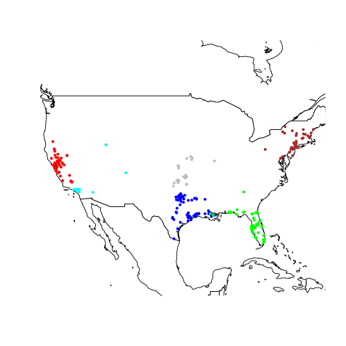
Figure 1. Sparse principal component analysis of ozone residuals from $444$ monitors across the U.S.. Depicted are the locations of the supports $\mathcal{S}_{1},\ldots,\mathcal{S}_{6}$ of the leading principal directions ${\bm{v}}_{1},\ldots,{\bm{v}}_{6}$.

The data of the years 2011 to 2014, providing the test sample ${\bm{Y}}_{n1},\ldots,{\bm{Y}}_{nn}$ with $n=1462$, was now analyzed using the leading directions as projection vectors. The proposed change-point tests were applied to test for the presence of changes in the (co-) variances ${\mathbb{C}}({\bm{v}}_{k}^{\top}{\bm{Y}}_{ni},{\bm{v}}_{\ell}^{\top}{\bm{Y}}_{ni})$, $i\in\{1,\ldots,n\}$, for $1\leq k\leq\ell\leq 7$. The asymptotic variance parameter was estimated using both the full in-sample and stopped-sample approach. The application of the unweighted CUSUM approach revealed no significances at the usual levels.

7. Proofs

The proofs are based on martingale approximations, which require several additional results and technical preparations. These results extend and complement the results obtained in [Steland and von Sachs, 2017].

7.1. Preliminaries

For an arbitray array of coefficients $\mathfrak{a}=\{a_{nj}^{(\nu)}:j\geq 0,1\leq\nu\leq d_{n},n\geq 1\}$ and vectors ${\bm{v}}_{n}=(v_{n1},\ldots,v_{nd_{n}})^{\top}$ and ${\bm{w}}_{n}=(w_{n1},\ldots,w_{nd_{n}})^{\top}$ with finite $\ell_{1}$-norm, i.e., $\|{\bm{v}}_{n}\|_{\ell_{1}},\|{\bm{w}}_{n}\|_{\ell_{1}}<\infty$, define

$$f_{0,0}^{(n)}(\mathfrak{a},{\bm{v}}_{n},{\bm{w}}_{n})=\sum_{\nu,\mu=1}^{d_{n}}v_{n\nu}w_{n\mu}a_{nj}^{(\nu)}a_{nj}^{(\mu)},\quad f_{l,j}^{(n)}(\mathfrak{a})=\sum_{\nu,\mu=1}^{d_{n}}v_{n\nu}w_{n\mu}[a_{nj}^{(\nu)}a_{n,j+l}^{(\mu)}+a_{nj}^{(\mu)}a_{n,j+l}^{(\nu)}]$$

for $j\in\{0,1,\cdots\}$ and $l\in\{1,2,\cdots\}$. Put $\widetilde{f}_{\ell,i}^{(n)}(\mathfrak{a},{\bm{v}}_{n},{\bm{w}}_{n})=\sum_{j=i}^{\infty}f_{\ell,j}^{(n)}(\mathfrak{a},{\bm{v}}_{n},{\bm{w}}_{n}),$ for $\ell,i\in\{0,1,2,\cdots\}$.

Introduce for coefficients $\mathfrak{a}$ satisfying Assumption (D) and vectors ${\bm{v}}_{n}$ and ${\bm{w}}_{n}$ the $\mathcal{F}_{nk}$-martingales

$$M_{k}^{(n)}(\mathfrak{a},{\bm{v}}_{n},{\bm{w}}_{n})=\widetilde{f}_{0,0}^{(n)}(\mathfrak{a},{\bm{v}}_{n},{\bm{w}}_{n})\sum_{i=0}^{k}(\epsilon_{ni}^{2}-\sigma_{i}^{2})+\sum_{i=0}^{k}\epsilon_{ni}\sum_{\ell=1}^{\infty}\widetilde{f}_{\ell,0}^{(n)}(\mathfrak{a},{\bm{v}}_{n},{\bm{w}}_{n})\epsilon_{n,i-j},\qquad k\geq 0,$$

which start in $M_{0}^{(n)}=0$, for each $n\geq 0$. Put

$$S_{n^{\prime},m^{\prime}}^{(n)}(\mathfrak{a},{\bm{v}}_{n},{\bm{w}}_{n})=\sum_{i=m^{\prime}+1}^{m^{\prime}+n^{\prime}}(Y_{ni}({\bm{v}}_{n}^{\top}{\bm{a}}_{n})Y_{ni}({\bm{w}}_{n}^{\top}{\bm{a}}_{n})-{\mathbb{E}}[Y_{ni}({\bm{v}}_{n}^{\top}{\bm{a}}_{n})Y_{ni}({\bm{w}}_{n}^{\top}{\bm{a}}_{n})]),\qquad m^{\prime},n^{\prime}\geq 0.$$

Notice that, by definitions (16) and (17),

(42) $$S_{k,0}^{(n)}(\mathfrak{b},{\bm{v}}_{n},{\bm{w}}_{n})={\bm{D}}_{nk}^{(1)},\qquad S_{k,0}^{(n)}(\mathfrak{c},{\bm{v}}_{n},{\bm{w}}_{n})={\bm{D}}_{nk}^{(2)},$$

for $k\geq 1$ and $n\geq 1$, where ${\bm{D}}_{nk}=({\bm{D}}_{nk}^{(1)},{\bm{D}}_{nk}^{(2)})$. For brevity introduce the difference operator

$$\delta M_{m^{\prime}+n^{\prime}}^{(n)}(\mathfrak{a},{\bm{v}}_{n},{\bm{w}}_{n}) =M_{m^{\prime}+n^{\prime}}^{(n)}(\mathfrak{a},{\bm{v}}_{n},{\bm{w}}_{n})-M_{m^{\prime}}^{(n)}(\mathfrak{a},{\bm{v}}_{n},{\bm{w}}_{n})$$

$$=\widetilde{f}_{0,0}^{(n)}(\mathfrak{a},{\bm{v}}_{n},{\bm{w}}_{n})\sum_{i=m^{\prime}+1}^{m^{\prime}+n^{\prime}}(\epsilon_{ni}^{2}-\sigma_{ni}^{2})+\sum_{i=m^{\prime}+1}^{m^{\prime}+n^{\prime}}\epsilon_{ni}\sum_{\ell=1}^{\infty}\widetilde{f}_{\ell,0}^{(n)}(\mathfrak{a},{\bm{v}}_{n},{\bm{w}}_{n})\epsilon_{n,i-\ell},$$

for $k,n\geq 1$, which takes the lag $n^{\prime}$ forward difference at $m^{\prime}$. Notice that for $m^{\prime}=0$

$$\delta M_{k}^{(n)}(\mathfrak{a},{\bm{v}}_{n},{\bm{w}}_{n})=\widetilde{f}_{0,0}^{(n)}(\mathfrak{a},{\bm{v}}_{n},{\bm{w}}_{n})\sum_{i=1}^{k}(\epsilon_{ni}^{2}-\sigma_{ni}^{2})+\sum_{i=1}^{k}\epsilon_{ni}\sum_{\ell=1}^{\infty}\widetilde{f}_{\ell,0}^{(n)}(\mathfrak{a},{\bm{v}}_{n},{\bm{w}}_{n})\epsilon_{n,i-\ell},\ k,n\geq 1,$$

coincides with the martingale $M_{k}^{(n)}(\mathfrak{a},{\bm{v}}_{n},{\bm{w}}_{n})$. A direct calculation shows that

(43) $${\mathbb{C}}(\delta M_{m^{\prime}+n^{\prime}}^{(n)}(\mathfrak{b},{\bm{v}}_{n},{\bm{w}}_{n}),\delta M_{m^{\prime}+n^{\prime}}^{(n)}(\mathfrak{c},\widetilde{{\bm{v}}}_{n},\widetilde{{\bm{w}}}_{n}))$$

$$\ =\widetilde{f}_{0,0}^{(n)}(\mathfrak{b},{\bm{v}}_{n},{\bm{w}}_{n})\widetilde{f}_{0,0}^{(n)}(\mathfrak{c},\widetilde{{\bm{v}}}_{n},\widetilde{{\bm{w}}}_{n})\sum_{j=1}^{n^{\prime}}(\gamma_{n,m^{\prime}+j}+\sigma_{n,m^{\prime}+j}^{4})$$

$$\qquad\qquad+\sum_{j=1}^{n^{\prime}}\sum_{\ell=1}^{\infty}\widetilde{f}_{\ell,0}^{(n)}(\mathfrak{b},{\bm{v}}_{n},{\bm{w}}_{n})\widetilde{f}_{\ell,0}^{(n)}(\mathfrak{c},\widetilde{{\bm{v}}}_{n},\widetilde{{\bm{w}}}_{n})\sigma_{n,m^{\prime}+j}^{2}\sigma_{n,m^{\prime}+j-\ell}^{2},$$

for $n^{\prime},m^{\prime}\geq 0$ and $n\geq 1$.

7.2. Martingale approximations

The following lemma provides an explicit formula for the asymptotic covariance parameter related to the two CUSUMs, $\beta_{n}^{2}(\mathfrak{b},{\bm{v}}_{n},{\bm{w}}_{n},\mathfrak{c},\widetilde{{\bm{v}}}_{n},\widetilde{{\bm{w}}}_{n})$, using different pairs $({\bm{v}}_{n},{\bm{w}}_{n})$ and $(\widetilde{{\bm{v}}}_{n},\widetilde{{\bm{w}}}_{n})$ of weighting vectors, abbreviated as $\beta_{n}^{2}(\mathfrak{b},\mathfrak{c})=\beta_{n}^{2}(\mathfrak{b},{\bm{v}}_{n},{\bm{w}}_{n},\mathfrak{c},{\bm{v}}_{n},{\bm{w}}_{n})$. Especially, it follows from these results that the asymptotic variance of a single CUSUM detector under the no-change null hypothesis, $\alpha^{2}(\mathfrak{a})=\beta_{n}^{2}(\mathfrak{a},\mathfrak{a})$, satisfies

$$\alpha_{n}^{2}(\mathfrak{a})\approx\frac{1}{n}{\mathbb{V}}(D_{nn}).$$

The following general results hold under a mild condition on the error terms and especially show that (73) can be approximated by $n^{\prime}\beta_{n}^{2}(\mathfrak{b},{\bm{v}}_{n},{\bm{w}}_{n},\mathfrak{c},\widetilde{{\bm{v}}}_{n},\widetilde{{\bm{w}}}_{n})$ at the rate $(n^{\prime})^{1-\theta}$, uniformly in $n$ and $m^{\prime}$, cf. [Steland and von Sachs, 2017, (3.18)] and [Kouritzin, 1995]. The proof extends these latter results and improves the bounds, but it is technical and thus deferred to the appendix. The improved bounds show that the $\ell_{1}$-norms of the weighting vectors may grow slowly without sacrificing the convergence of the second moments, cf. the verification of (II) and (III) in the proof of Theorem 1.

Lemma 1.

Let $\epsilon_{ni}$, $i\in\mathbb{Z}$, be independent with variances $\sigma_{ni}^{2}$ and third moments $\gamma_{ni}$ satisfying

(44) $$\frac{1}{n^{\prime}}\sum_{i=1}^{n^{\prime}}i|\sigma_{ni}^{2}-s_{n1}^{2}|\stackrel{{\scriptstyle n,n^{\prime}}}{{\ll}}(n^{\prime})^{-\beta},$$

(45) $$\frac{1}{n^{\prime}}\sum_{i=1}^{n^{\prime}}i|\gamma_{ni}-\gamma_{n}|\stackrel{{\scriptstyle n,n^{\prime}}}{{\ll}}(n^{\prime})^{-\beta}$$

for constants $s_{n1}^{2}\in(0,\infty)$ and $\gamma_{n}\in\mathbb{R}$ for some $1<\beta<2$ with $1+\theta<\beta$. Then for $n,n^{\prime}\geq 1$, with $K_{n}=\|{\bm{v}}_{n}\|_{\ell_{1}}\|{\bm{w}}_{n}\|_{\ell_{1}}\|\widetilde{{\bm{v}}}_{n}\|_{\ell_{1}}\|\widetilde{{\bm{v}}}_{n}\|_{\ell_{1}}$,

(46) $$\left|{\mathbb{C}}(M_{n^{\prime}}^{(n)}(\mathfrak{b},{\bm{v}}_{n},{\bm{w}}_{n}),M_{n^{\prime}}^{(n)}(\mathfrak{c},\widetilde{{\bm{v}}}_{n},\widetilde{{\bm{w}}}_{n}))-(n^{\prime})\beta_{n}^{2}(\mathfrak{b},{\bm{v}}_{n},{\bm{w}}_{n},\mathfrak{c},\widetilde{{\bm{v}}}_{n},\widetilde{{\bm{w}}}_{n})\right|\stackrel{{\scriptstyle n,n^{\prime}}}{{\ll}}K_{n}(n^{\prime})^{1-\theta},$$

and for $n,n^{\prime}\geq 1$ and $m^{\prime}\geq 0$

(47) $$\left|{\mathbb{C}}(\delta M_{m^{\prime}+n^{\prime}}^{(n)}(\mathfrak{b},{\bm{v}}_{n},{\bm{w}}_{n}),\delta M_{m^{\prime}+n^{\prime}}^{(n)}(\mathfrak{c},\widetilde{{\bm{v}}}_{n},\widetilde{{\bm{w}}}_{n}))-(n^{\prime})\beta_{n}^{2}(\mathfrak{b},{\bm{v}}_{n},{\bm{w}}_{n},\mathfrak{c},\widetilde{{\bm{v}}}_{n},\widetilde{{\bm{w}}}_{n})\right|\stackrel{{\scriptstyle n,n^{\prime},m^{\prime}}}{{\ll}}K_{n}(n^{\prime})^{1-\theta},$$

if

(48) $$\beta_{n}^{2}(\mathfrak{b},{\bm{v}}_{n},{\bm{w}}_{n},\mathfrak{c},\widetilde{{\bm{v}}}_{n},\widetilde{{\bm{w}}}_{n})=\widetilde{f}_{0,0}^{(n)}(\mathfrak{b},{\bm{v}}_{n},{\bm{w}}_{n})\widetilde{f}_{0,0}^{(n)}(\mathfrak{c})(\gamma_{n}-s_{n1}^{4})+s_{n1}^{4}\sum_{\ell=1}^{\infty}\widetilde{f}_{\ell,0}^{(n)}(\mathfrak{b},{\bm{v}}_{n},{\bm{w}}_{n})\widetilde{f}_{\ell,0}^{(n)}(\mathfrak{c},\widetilde{{\bm{v}}}_{n},\widetilde{{\bm{w}}}_{n}).$$

Lemma 2.

Let $\{\epsilon_{nk}:k\geq 1,n\geq 1\}$ be independent mean zero random variables with variances $\sigma_{nk}^{2}$ and third moments $\gamma_{nk}$ satisfying Assumption (E). Let $\mathfrak{a}$ be coefficients satisfying the decay condition (D). Then we have for $n^{\prime},m^{\prime}\geq 0$ and $n\geq 1$

(49) $${\mathbb{E}}(S_{n^{\prime},m^{\prime}}^{(n)}(\mathfrak{a},{\bm{v}}_{n},{\bm{w}}_{n})-\delta M_{m^{\prime}+n^{\prime}}^{(n)}(\mathfrak{a},{\bm{v}}_{n},{\bm{w}}_{n}))^{2}\stackrel{{\scriptstyle n,m^{\prime},n^{\prime}}}{{\ll}}\|{\bm{v}}_{n}\|_{\ell_{1}}^{2}\|{\bm{w}}_{n}\|_{\ell_{1}}^{2}(n^{\prime})^{1-\theta}.$$

Further, for $k\geq 1$ and $n\geq 1$

(50) $${\mathbb{E}}({\bm{D}}_{nk}^{(1)}-\delta M_{k}^{(n)}(\mathfrak{b}))^{2} \stackrel{{\scriptstyle n,k}}{{\ll}}\|{\bm{v}}_{n}\|_{\ell_{1}}^{2}\|{\bm{w}}_{n}\|_{\ell_{1}}^{2}k^{1-\theta},$$

(51) $${\mathbb{E}}({\bm{D}}_{nk}^{(2)}-\delta M_{k}^{(n)}(\mathfrak{c}))^{2} \stackrel{{\scriptstyle n,k}}{{\ll}}\|{\bm{v}}_{n}\|_{\ell_{1}}^{2}\|{\bm{w}}_{n}\|_{\ell_{1}}^{2}k^{1-\theta},$$

such that

(52) $${\mathbb{E}}\|{\bm{D}}_{nk}-\delta{\bm{M}}_{k}^{(n)}\|_{2}^{2}\stackrel{{\scriptstyle n,k}}{{\ll}}\|{\bm{v}}_{n}\|_{\ell_{1}}^{2}\|{\bm{w}}_{n}\|_{\ell_{1}}^{2}n^{1-\theta}.$$

(50), (51) and (52) also hold (with obvious modifications), if ${\bm{D}}_{nk}^{(1)}=S_{k,0}^{(n)}(\mathfrak{b},{\bm{v}}_{n},{\bm{w}}_{n})$ and ${\bm{D}}_{nk}^{(2)}=S_{k,0}^{(n)}(\mathfrak{c},\widetilde{{\bm{v}}}_{n},\widetilde{{\bm{w}}}_{n})$ for two pairs of weighting vectors, where the bound in (52) then is given by $\max\{\|{\bm{v}}_{n}\|_{\ell_{1}}^{2}\|{\bm{w}}_{n}\|_{\ell_{1}}^{2},\|\widetilde{{\bm{v}}}_{n}\|_{\ell_{1}}^{2}\|\widetilde{{\bm{w}}}_{n}\|_{\ell_{1}}^{2}\}n^{1-\theta}$.

Proof.

See appendix. ∎

The next lemma studies the conditional covariances of the approximating martingales. It generalizes [Steland and von Sachs, 2018, Lemma 2.2] to the change-point model and two different pairs of projection vectors.

Lemma 3.

Suppose that the conditions of Lemma 1 hold and $\beta_{n}^{2}(\mathfrak{b},\mathfrak{c})$ is as defined there. Then it holds for $m^{\prime},n^{\prime}\geq 0$ and $n\geq 1$ with $K_{n}=\|{\bm{v}}_{n}\|_{\ell_{1}}\|{\bm{w}}_{n}\|_{\ell_{1}}\|\widetilde{{\bm{v}}}_{n}\|_{\ell_{1}}\|\widetilde{{\bm{w}}}_{n}\|_{\ell_{1}}$

$$E_{n^{\prime}}^{(n)} =\left\|{\mathbb{E}}\left[(\delta M_{m^{\prime}+n^{\prime}}^{(n)}(\mathfrak{b},{\bm{v}}_{n},{\bm{w}}_{n}))(\delta M_{m^{\prime}+n^{\prime}}^{(n)}(\mathfrak{c},\widetilde{{\bm{v}}}_{n},\widetilde{{\bm{w}}}_{n}))\mid\mathcal{F}_{n,m^{\prime}}\right]-n^{\prime}\beta_{n}^{2}(\mathfrak{b},{\bm{v}}_{n},{\bm{w}}_{n},\mathfrak{c},\widetilde{{\bm{v}}}_{n},\widetilde{{\bm{w}}}_{n})\right\|_{L_{1}}$$

$$\stackrel{{\scriptstyle n,m^{\prime},n^{\prime}}}{{\ll}}K_{n}(n^{\prime})^{1-\theta/2}$$

and

$$\left\|{\mathbb{E}}\left[(S_{m^{\prime},n^{\prime}}^{(n)}(\mathfrak{b},{\bm{v}}_{n},{\bm{w}}_{n}))(S_{m^{\prime},n^{\prime}}^{(n)}(\mathfrak{c},\widetilde{{\bm{v}}}_{n},\widetilde{{\bm{w}}}_{n}))\mid\mathcal{F}_{n,m^{\prime}}\right]-n^{\prime}\beta_{n}^{2}(\mathfrak{b},{\bm{v}}_{n},{\bm{w}}_{n},\mathfrak{c},\widetilde{{\bm{v}}}_{n},\widetilde{{\bm{w}}}_{n})\right\|_{L_{1}}$$

$$\stackrel{{\scriptstyle n,m^{\prime},n^{\prime}}}{{\ll}}K_{n}(n^{\prime})^{1-\theta/2}.$$

Proof.

See appendix. ∎

7.3. Proofs of Subsection 3.2

After the above preparations, we are now in a position to show Theorem 1.

Proof of Theorem 1.

Put

(53) $$\bm{\xi}_{i}^{(n)}=\bm{\xi}_{i}^{(n)}({\bm{v}}_{n}^{\top}{\bm{b}}_{n},{\bm{v}}_{n}^{\top}{\bm{c}}_{n})=\left(\begin{array}[]{cc}Y_{ni}({\bm{v}}_{n}^{\top}{\bm{b}}_{n})Y_{ni}({\bm{w}}_{n}^{\top}{\bm{b}}_{n})-{\mathbb{E}}[Y_{ni}({\bm{v}}_{n}^{\top}{\bm{b}}_{n})Y_{ni}({\bm{w}}_{n}^{\top}{\bm{b}}_{n})]\\ Y_{ni}({\bm{v}}_{n}^{\top}{\bm{c}}_{n})Y_{ni}({\bm{w}}_{n}^{\top}{\bm{c}}_{n})-{\mathbb{E}}[Y_{ni}({\bm{v}}_{n}^{\top}{\bm{c}}_{n})Y_{ni}({\bm{w}}_{n}^{\top}{\bm{c}}_{n})]\end{array}\right),$$

such that ${\bm{D}}_{nk}=\sum_{i\leq k}\bm{\xi}_{i}^{(n)},$ for $k\geq 1$ and $n\geq 1$. Let us consider the bivariate extension of the sums $S_{n^{\prime},m^{\prime}}^{(n)}$,

$${\bm{S}}_{n^{\prime},m^{\prime}}^{(n)}=(S_{n^{\prime},m^{\prime}}^{(n)}(1),S_{n^{\prime},m^{\prime}}^{(n)}(2))^{\top}=\sum_{k=m^{\prime}+1}^{m^{\prime}+n^{\prime}}\bm{\xi}_{k}^{(n)},\qquad m^{\prime},n^{\prime}\geq 0.$$

Introduce the conditional covariance operators

$${\bm{C}}_{n^{\prime},m^{\prime}}^{(n)}({\bm{u}})={\mathbb{E}}[{\bm{u}}^{\top}S_{n^{\prime},m^{\prime}}^{(n)}S_{n^{\prime},m^{\prime}}^{(n)}|\mathcal{F}_{n,m^{\prime}}],\qquad{\bm{u}}\in\mathbb{R}^{2},\ n,n^{\prime},m^{\prime}\geq 1,$$

and the unconditional covariance operator associated to the Brownian motion ${\bm{B}}^{(n)}$,

$${\bm{T}}^{(n)}({\bm{u}})={\mathbb{E}}({\bm{u}}^{\top}{\bm{B}}_{n}{\bm{B}}_{n}),\qquad{\bm{u}}\in\mathbb{R}^{2},\ n\geq 1.$$

We shall verify [Philipp, 1986, Th. 1], namely the validity of the following conditions: For $m^{\prime}\geq 0$, $n^{\prime}\geq 1$,

• $\sup_{j\geq 1}{\mathbb{E}}\|\bm{\xi}_{j}^{(n)}\|_{2}^{2+\delta}<\infty$ for some $\delta>0$.

• For some $\varepsilon>0$ it holds

  $${\mathbb{E}}\|{\mathbb{E}}({\bm{S}}_{n^{\prime},m^{\prime}}^{(n)}\mid\mathcal{F}_{n,m^{\prime}})\|_{2}\stackrel{{\scriptstyle n,n^{\prime},m^{\prime}}}{{\ll}}(n^{\prime})^{1/2-\varepsilon}$$

• There exists a covariance operator ${\bm{C}}$, namely ${\bm{T}}^{(n)}$, such that the conditional covariance operator ${\bm{C}}_{n^{\prime},m^{\prime}}^{(n)}$ converges to ${\bm{C}}$ in the semi-norm $\|\cdot\|_{op}$ in expectation in the sense that for some $\theta^{\prime}>0$.

  $${\mathbb{E}}\|{\bm{C}}_{n^{\prime}}(\cdot\mid\mathcal{F}_{n,m^{\prime}})-{\bm{C}}(\cdot)\|_{op}\stackrel{{\scriptstyle n,n^{\prime},m^{\prime}}}{{\ll}}(n^{\prime})^{1-\theta^{\prime}}.$$

Remark: As the construction is for fixed $n$, one could consider $\stackrel{{\scriptstyle n^{\prime},m^{\prime}}}{{\ll}}$ in (II) and (III). But since we are interested in $n\to\infty$ and (II) and (III) yield the moment convergence with rate for the partial sum ${\bm{S}}_{n,0}^{(n)}$ of interest (for large $n$), we show $\stackrel{{\scriptstyle n,n^{\prime},m^{\prime}}}{{\ll}}$ and consider the case $n^{\prime}\geq n$. This includes the real sample size $n$ and (21) then ensures the bound $\|{\bm{v}}_{n}\|_{\ell_{1}}^{2}\|{\bm{w}}_{n}\|_{\ell_{1}}^{2}(n^{\prime})^{-\theta/2}=O((n^{\prime})^{-\theta^{\prime}/2})$ we shall use.

Write $\bm{\xi}_{i}^{(n)}=(\bm{\xi}_{i1}^{(n)},\bm{\xi}_{i2}^{(n)})^{\top}$, $i\geq 1$, and observe that $\bm{\xi}_{ij}^{(n)}=\|{\bm{v}}_{n}\|_{\ell_{1}}\|{\bm{w}}\|_{\ell_{1}}\bm{\xi}_{nij}^{*}$ where $\bm{\xi}_{nij}^{*}$ is obtained from $\bm{\xi}_{ij}^{(n)}$ by replacing ${\bm{v}}_{n}$ by ${\bm{v}}_{n}^{*}={\bm{v}}_{n}/\|{\bm{v}}_{n}\|_{\ell_{1}}$ and ${\bm{w}}_{n}$ by ${\bm{w}}_{n}^{*}={\bm{w}}_{n}/\|{\bm{w}}_{n}\|_{\ell_{1}}$. The $C_{r}$-inequality and Cauchy-Schwarz yield

$${\mathbb{E}}|\bm{\xi}_{i1}^{(n)}|^{2+\delta} \leq\|{\bm{v}}_{n}\|_{\ell_{1}}^{2+\delta}\|{\bm{w}}_{n}\|_{\ell_{1}}^{2+\delta}{\mathbb{E}}(|Y_{ni}({\bm{v}}_{n}^{*}{}^{\top}{\bm{b}}_{n})Y_{ni}({\bm{w}}_{n}^{*}{}^{\top}{\bm{b}}_{n})|+{\mathbb{E}}|Y_{ni}({\bm{v}}_{n}^{*}{}^{\top}{\bm{b}}_{n})Y_{ni}({\bm{w}}_{n}^{*}{}^{\top}{\bm{b}}_{n})|)^{2+\delta}$$

$$\leq\|{\bm{v}}_{n}\|_{\ell_{1}}^{2+\delta}\|{\bm{w}}_{n}\|_{\ell_{1}}^{2+\delta}2^{3+\delta}{\mathbb{E}}|Y_{ni}({\bm{v}}_{n}^{*}{}^{\top}{\bm{b}}_{n})Y_{ni}({\bm{w}}_{n}^{*}{}^{\top}{\bm{b}}_{n})|^{2+\delta}$$

$$\leq\|{\bm{v}}_{n}\|_{\ell_{1}}^{2+\delta}\|{\bm{w}}_{n}\|_{\ell_{1}}^{2+\delta}2^{3+\delta}\sqrt{{\mathbb{E}}|Y_{ni}({\bm{v}}_{n}^{*}{}^{\top}{\bm{b}}_{n})|^{4+2\delta}}\sqrt{{\mathbb{E}}|Y_{ni}({\bm{w}}_{n}^{*}{}^{\top}{\bm{b}}_{n})|^{4+2\delta}},$$

and the second component is estimated analogously. Following the arguments in [Kouritzin, 1995, p. 343], for $\delta^{\prime}\in(0,2)$ and $\chi=\delta^{\prime}/2$, one can show that for $\mathfrak{a}\in\{\mathfrak{b},\mathfrak{c}\}$ and ${\bm{u}}_{n}\in\{{\bm{v}}_{n}^{*},{\bm{w}}_{n}^{*}\}$

$${\mathbb{E}}|Y_{ni}({\bm{u}}_{n}^{\prime}{\bm{a}}_{n})|^{4+\delta^{\prime}} \leq\sup_{n,k\geq 0}{\mathbb{E}}|\epsilon_{nk}|\sum_{\ell=0}^{\infty}|a_{n\ell}^{(u)}|^{2(2+\chi)}$$

$$+\sup_{n,k\geq 0}{\mathbb{E}}(\epsilon_{nk}^{2})\left\{\sup_{n^{\prime},k^{\prime}\geq 0}{\mathbb{E}}(\epsilon_{n^{\prime}k^{\prime}}^{2})\right\}^{1+\chi}\sum_{\ell=0}^{\infty}|a_{n\ell}^{(u)}|^{2}\left\{\sum_{\ell=0}^{\infty}|a_{n\ell}^{(u)}|^{2}\right\}^{1+\chi},$$

where $a_{n\ell}^{(u)}=\sum_{\nu=1}^{d_{n}}a_{n\ell}^{(\nu)}u_{n\nu}\ll(\max(\ell,1))^{-3/4-\theta/2}$, uniformly in uniformly $\ell_{1}$-bounded ${\bm{u}}_{n}$ and $n\geq 1$, such that $\sum_{\ell=0}^{\infty}|a_{n\ell}^{(u)}|^{2}<\infty$ and, in turn, $\sum_{\ell=0}^{\infty}|a_{n\ell}^{(u)}|^{2(2+\chi)}<\infty$. Eventually, we obtain for any $n$

(54) $$\max_{j=1,2}\sup_{i\geq 1}{\mathbb{E}}|\bm{\xi}_{ij}^{(n)}|^{2+\delta}=O(\|{\bm{v}}_{n}\|_{\ell_{1}}^{2+\delta}\|{\bm{w}}_{n}\|_{\ell_{1}}^{2+\delta}).$$

Now Jensen’s inequality yields

$${\mathbb{E}}\|\bm{\xi}_{i}^{(n)}\|_{2}^{2+\delta}=2^{1+\delta/2}{\mathbb{E}}\left(\frac{1}{2}\sum_{j=1,2}[\bm{\xi}_{ij}^{(n)}]^{2}\right)^{1+\delta/2}\leq 2^{\delta/2}\sum_{j=1,2}{\mathbb{E}}|\bm{\xi}_{ij}^{(n)}|^{2+\delta}<\infty,$$

verifying (I). To show (II) recall that the martingale approximation for ${\bm{S}}_{n^{\prime},m^{\prime}}^{(n)}=(S_{n^{\prime},m^{\prime}}^{(n)}(\mathfrak{b}),S_{n^{\prime},m^{\prime}}^{(n)}(\mathfrak{c}))^{\top}$ is given by $\delta{\bm{M}}_{n^{\prime},m^{\prime}}^{(n)}=(\delta M_{m^{\prime}+n^{\prime}}^{(n)}(\mathfrak{b}),\delta M_{m^{\prime}+n^{\prime}}^{(n)}(\mathfrak{c}))^{\top},$ see Lemma 2. Using

$${\mathbb{E}}(\delta M_{m^{\prime}+n^{\prime}}^{(n)}(\mathfrak{b})\mid\mathcal{F}_{n,m^{\prime}})=0,\ \text{and hence}\ {\mathbb{E}}({\bm{S}}_{n^{\prime},m^{\prime}}^{(n)}\mid\mathcal{F}_{n,m^{\prime}})={\mathbb{E}}({\bm{S}}_{n^{\prime},m^{\prime}}^{(n)}-\delta{\bm{M}}_{n^{\prime},m^{\prime}}^{(n)}\mid\mathcal{F}_{n,m^{\prime}}),$$

it follows that

$${\mathbb{E}}\|{\mathbb{E}}({\bm{S}}_{n^{\prime},m^{\prime}}^{(n)}\mid\mathcal{F}_{n,m^{\prime}})\|_{2}\stackrel{{\scriptstyle n,n^{\prime},m^{\prime}}}{{\ll}}\|{\bm{v}}_{n}\|_{\ell_{1}}^{2}\|{\bm{w}}_{n}\|_{\ell_{1}}^{2}(n^{\prime})^{1/2-\theta/2}\stackrel{{\scriptstyle n,n^{\prime},m^{\prime}}}{{\ll}}(n^{\prime})^{1/2-\theta^{\prime}/2},$$

by Lemma 2 and (21), such that (II) holds with $\varepsilon=\theta^{\prime}/2$. It remains to show (III). Observe that

$$\left\|\frac{1}{n^{\prime}}{\bm{C}}_{n^{\prime},m^{\prime}}^{(n)}-{\bm{T}}^{(n)}\right\|_{op}$$

$$\qquad=\sup_{{\bm{u}}\in\mathbb{R}^{2},\|{\bm{u}}\|_{2}=1}\left|{\bm{u}}^{\top}{\mathbb{E}}\left[\frac{{\bm{S}}_{n^{\prime},m^{\prime}}^{(n)}}{\sqrt{n^{\prime}}}\frac{{\bm{S}}_{n^{\prime},m^{\prime}}^{(n)}{}^{\top}}{\sqrt{n^{\prime}}}\mid\mathcal{F}_{n,m^{\prime}}\right]{\bm{u}}-\sum_{j=1,2}u_{j}\left(\begin{array}[]{cc}{\mathbb{C}}(B_{n1},B_{nj})\\ {\mathbb{C}}(B_{n2},B_{nj})\end{array}\right)^{\top}{\bm{u}}\right|$$

$$\qquad=\sup_{{\bm{u}}\in\mathbb{R}^{2},\|{\bm{u}}\|_{2}=1}\left|\sum_{i,j=1}^{2}u_{i}u_{j}\left({\mathbb{E}}\left[\frac{S_{n^{\prime},m^{\prime}}^{(n)}(i)}{\sqrt{n^{\prime}}}\frac{S_{n^{\prime},m^{\prime}}^{(n)}(j)}{\sqrt{n^{\prime}}}\mid\mathcal{F}_{n,m^{\prime}}\right]-{\mathbb{C}}(B_{ni},B_{nj})\right)\right|.$$

Noting that $|u_{i}u_{j}|\leq\max_{k}u_{k}^{2}\leq 1$, we obtain

$$\left\|\frac{1}{n^{\prime}}{\bm{C}}_{n^{\prime},m^{\prime}}^{(n)}-{\bm{T}}^{(n)}\right\|_{op}\leq 4\max_{1\leq i,j\leq 2}\left|{\mathbb{E}}\left[\frac{S_{n^{\prime},m^{\prime}}^{(n)}(i)}{\sqrt{n^{\prime}}}\frac{S_{n^{\prime},m^{\prime}}^{(n)}(j)}{\sqrt{n^{\prime}}}\mid\mathcal{F}_{n,m^{\prime}}\right]-{\mathbb{C}}(B_{ni},B_{nj})\right|.$$

Therefore, (III) follows, if

$${\mathbb{E}}\left|{\mathbb{E}}\left[\frac{S_{n^{\prime},m^{\prime}}^{(n)}(i)}{\sqrt{n^{\prime}}}\frac{S_{n^{\prime},m^{\prime}}^{(n)}(j)}{\sqrt{n^{\prime}}}\mid\mathcal{F}_{n,m^{\prime}}\right]-{\mathbb{C}}(B_{ni},B_{nj})\right|\stackrel{{\scriptstyle n,n^{\prime},m^{\prime}}}{{\ll}}\|{\bm{v}}_{n}\|_{\ell_{1}}^{2}\|{\bm{w}}_{n}\|_{\ell_{1}}^{2}(n^{\prime})^{-\theta/2},$$

a.s., which is shown in Lemma 3, since then assumption (21) ensures the estimate $\stackrel{{\scriptstyle n,n^{\prime},m^{\prime}}}{{\ll}}(n^{\prime})^{-\theta^{\prime}/2}$. Hence, from [Philipp, 1986], we may conclude that there exists a constant $C_{n}$ and a universal constant $\lambda>0$, such that

(55) $$\|{\bm{D}}_{nt}-{\bm{B}}_{n}(t)\|_{2}\leq C_{n}t^{1/2-\lambda}\qquad t>0,$$

a.s., which implies

(56) $$|{\bm{D}}_{nt}^{(i)}-{\bm{B}}_{n}^{(i)}(t)|\leq\sqrt{2}C_{n}t^{1/2-\lambda},\qquad t>0,$$

a.s., for $i=1,2$. Recalling that $D_{nt}={\bm{v}}_{n}^{\top}({\bm{S}}_{nt}-{\mathbb{E}}({\bm{S}}_{nt})){\bm{w}}_{n}$ where ${\bm{S}}_{nt}=\sum_{i\leq t}{\bm{Y}}_{ni}{\bm{Y}}_{ni}^{\top}$ satisfies

$${\bm{S}}_{nt} ={\bm{1}}(t\leq\tau)\sum_{i\leq t}{\bm{Y}}_{ni}(\mathfrak{b}){\bm{Y}}_{ni}(\mathfrak{b})^{\top}+{\bm{1}}(t>\tau)\left[\sum_{i\leq\tau}{\bm{Y}}_{ni}(\mathfrak{b}){\bm{Y}}_{ni}(\mathfrak{b})^{\top}+\sum_{i=\tau+1}^{t}{\bm{Y}}_{ni}(\mathfrak{c}){\bm{Y}}_{ni}(\mathfrak{c})^{\top}\right],$$

we have the following crucial representation in terms of ${\bm{D}}_{nt}$,

$$D_{nt}={\bm{D}}_{nt}^{(1)}{\bm{1}}(t\leq\tau)+[{\bm{D}}_{n\tau}^{(1)}+{\bm{D}}_{nt}^{(2)}-{\bm{D}}_{n\tau}^{(2)}]{\bm{1}}(t>\tau),$$

for all $t$. Since

$$D_{nt}-\{{\bm{B}}_{n}^{(1)}(t){\bm{1}}(t\leq\tau)+[{\bm{B}}_{n}^{(1)}(\tau)+{\bm{B}}_{n}^{(2)}(t)-{\bm{B}}_{n}^{(2)}(\tau)]\}$$

$$=\quad\left({\bm{D}}_{nt}^{(1)}-{\bm{B}}_{n}^{(1)}(t)\right){\bm{1}}(t\leq\tau)+\left({\bm{D}}_{n\tau}^{(1)}-{\bm{B}}_{n}^{(1)}(\tau)+{\bm{D}}_{nt}^{(2)}-{\bm{B}}_{n}^{(2)}(t)-{\bm{D}}_{nt}^{(2)}(\tau)+{\bm{B}}_{n}^{(2)}(\tau)\right){\bm{1}}(t>\tau),$$

(56) yields, by definition of $G_{n}$, see (19),

$$|D_{nt}-G_{n}(t)| =|D_{nt}-\{{\bm{B}}_{n}^{(1)}(t){\bm{1}}(t\leq\tau)+[{\bm{B}}_{n}^{(1)}(\tau)+{\bm{B}}_{n}^{(2)}(t)-{\bm{B}}_{n}^{(2)}(\tau)]\}|\leq 3\sqrt{2}C_{n}t^{1/2-\lambda},$$

for $t>0$, a.s.. This implies

(57) $$\frac{1}{\sqrt{n}}\max_{1\leq k<n}|D_{nk}-G_{n}(k)|\leq\frac{1}{\sqrt{n}}C_{n}\max_{1\leq k<n}k^{1/2-\lambda}\leq 3\sqrt{2}C_{n}n^{-\lambda},$$

as $n\to\infty$, a.s., which in turn leads to (iii), since

$$\frac{1}{\sqrt{n}}\max_{1\leq k<n}\left|D_{nk}-\frac{k}{n}D_{nn}-G_{n}^{0}(k)\right| =\frac{1}{\sqrt{n}}\max_{1\leq k<n}\left|D_{nk}-\frac{k}{n}D_{nn}-\left[G_{n}(k)-\frac{k}{n}G_{n}(n)\right]\right|\leq 6\sqrt{2}C_{n}n^{-\lambda},$$

as $n\to\infty$, a.s., and (iv) follows from the reverse triangle inequality. Recalling that $U_{nk}={\mathbb{E}}(U_{nk})+D_{nk}$ and $U_{nk}-\frac{k}{n}U_{nn}=m_{n}(k)+D_{nk}-\frac{k}{n}D_{nn}$, we obtain

$$\frac{1}{\sqrt{n}}\max_{1\leq k<n}\left|U_{nk}-\frac{k}{n}U_{nn}-\left[m_{n}(k)+G_{n}^{0}(k)\right]\right|\leq 6\sqrt{2}C_{n}n^{-\lambda},$$

as $n\to\infty$, a.s., which shows (v). (vi) now follows easily from the reverse triangle inequality. For a weight function $g$ satisfying (13) the arguments are more involved and as follows: Let $\gamma_{n}$ be a non-decreasing sequence specified later. Then, using $g(t)/[t(1-t)]^{\beta}\geq C_{g}$ and $n^{2}/(k(n-k))\leq 2n/k$ for $1\leq k\leq n/2$, we obtain a.s.

$$\max_{\varepsilon n/\gamma_{n}\leq k\leq n/2}\frac{1}{\sqrt{n}g(k/n)}\left|D_{nk}-\frac{k}{n}D_{nn}-G_{n}^{0}(k)\right|$$

$$\qquad\leq C_{g}^{-1}\max_{\varepsilon n/\gamma_{n}\leq k\leq n/2}\left(\frac{n}{k}\frac{n}{n-k}\right)^{\beta}\frac{1}{\sqrt{n}}\left|D_{nk}-\frac{k}{n}D_{nn}-G_{n}^{0}(k)\right|$$

$$\qquad\leq C_{g}^{-1}(2/\varepsilon)^{\beta}\gamma_{n}^{\beta}\max_{1\leq k<n}\frac{1}{\sqrt{n}}\left|D_{nk}-\frac{k}{n}D_{nn}-G_{n}^{0}(k)\right|$$

$$\qquad\leq 3\sqrt{2}C_{g}^{-1}(2/\varepsilon)^{\beta}\gamma_{n}^{\beta}C_{n}n^{-\lambda}.$$

The maximum over $n/2\leq k\leq(1-\varepsilon/\gamma_{n})n$ is estimated analogously leading to

$$\max_{\varepsilon n/\gamma_{n}\leq k\leq(1-\varepsilon/\gamma_{n})n}\left(\frac{n}{k}\frac{n}{n-k}\right)^{\beta}\frac{1}{\sqrt{n}}\left|D_{nk}-\frac{k}{n}D_{nn}-G_{n}^{0}(k)\right|=O(\gamma_{n}^{\beta}C_{n}n^{-\lambda}),a.s..$$

The right-hand side is $o(1)$, a.s., if we put $\gamma_{n}=n^{0.1\lambda/\beta}$. Further, the technical results of the appendix and the Hájek-Rényi inequality for martingale differences yield for any $\delta>0$ the tail bound

$${\mathbb{P}}\left(\max_{1\leq k\leq n\varepsilon/\gamma_{n}}\left(\frac{n}{k}\right)^{\beta}\frac{1}{\sqrt{n}}\left|D_{nk}-\frac{k}{n}D_{nn}\right|\geq\delta\right) =O\left(\frac{n^{2\beta-1}}{(\delta/2)^{2}}\sum_{k=1}^{n\varepsilon/\gamma_{n}}k^{-2\beta}\right)+O\left(\frac{n^{1-\theta}}{\delta^{2}n}\right)$$

$$=O\left((\varepsilon)^{1-2\beta}\gamma_{n}^{2\beta-1}(\log(n\varepsilon/\gamma_{n})+1)^{2\beta}\right)+o(1)$$

$$=O\left((\varepsilon)^{1-2\beta}n^{0.1(2\beta-1)\lambda/\beta}(\log(n)+1)^{2\beta}\right)+o(1).$$

The first term tends to $0$, as $\varepsilon\to 0$, uniformly in $n$, since $\beta<1/2$. Let $B^{0}$ be a Brownian bridge and note that $\{\alpha_{n}^{-1}(\mathfrak{b})\overline{G}_{n}^{0}(t):0\leq t\leq\vartheta\}\stackrel{{\scriptstyle d}}{{=}}\{B^{0}(t):0\leq t\leq\vartheta\}$. Using the estimates $\sqrt{t}/t^{\beta}\leq(\varepsilon/\gamma_{n})^{1/2-\beta}$ and $\log_{2}(1/t)\leq\log_{2}(n)$ on $t\in\mathcal{G}_{n}=\{1/n,\dots,\lfloor\varepsilon n/\gamma_{n}\rfloor/n\}$ the law of the iterated logarithm for the Brownian bridge, [Shorack and Wellner, 1986, p.72], entails for $\delta>0$ and $\varepsilon/\gamma_{n}\leq\vartheta$ (thus for large $n$)

$${\mathbb{P}}\left(\max_{1\leq k\leq n\varepsilon/\gamma_{n}}\left(\frac{n}{k}\right)^{\beta}\frac{|n^{-1/2}G_{n}^{0}(k)|}{\alpha_{n}(\mathfrak{b})}>\delta\right) \leq{\mathbb{P}}\left(\sup_{t\in\mathcal{G}_{n}}\frac{|B^{0}(t)|}{\sqrt{2t\log_{2}(1/t)}}>\frac{\delta}{\alpha_{n}(\mathfrak{b})\sqrt{2\log_{2}(n)}(\varepsilon/\gamma_{n})^{1/2-\beta}}\right)$$

$$=o(1),$$

by our choice of $\gamma_{n}$ and since $\beta<1/2$. The corresponding tail probabilities for the maximum over $(1-\varepsilon/\gamma_{n})n\leq k\leq n$ are treated analogously. Combining the above estimates shows (22). ∎

Proof of Theorem 2.

See appendix. ∎

Proof of Theorem 3.

See appendix. ∎

Proof of Theorem 4.

Since $\widetilde{{\bm{v}}}_{n}=a_{n}^{-1}{\bm{v}}_{n}$ and $\widetilde{{\bm{w}}}_{n}=b_{n}^{-1}{\bm{w}}_{n}$ satisfy property (21) and

$$D_{nk}(g;a_{n}^{-1}{\bm{v}}_{n},b_{n}^{-1}{\bm{w}}_{n})=a_{n}^{-1}b_{n}^{-1}D_{nk}(g;{\bm{v}}_{n},{\bm{w}}_{n}),$$

we may conclude that $T_{n}(g;{\bm{v}}_{n},{\bm{w}}_{n})=T_{n}(g;\widetilde{{\bm{v}}}_{n},\widetilde{{\bm{w}}}_{n})$. Consequently, all approximations for $T_{n}$ carry over. In particular, we obtain under the conditions of Theorem 1, cf. (23),

$$\left|T_{n}(g;{\bm{v}}_{n},{\bm{w}}_{n})-\max_{1\leq k<n}\frac{1}{g(k/n)}\biggl{|}\frac{m_{n}(k)}{\sqrt{n}}+\overline{B}_{n}^{0}(k/n)\biggr{|}\right|=o_{{\mathbb{P}}}(1).$$

Note that $\overline{B}_{n}=\alpha_{n}^{-1}(\mathfrak{b})\overline{G}_{n}^{0}(t)$ is a standard Brownian on $[0,\vartheta]$, cf. (20), whereas the scale factor changes from $1$ to $\alpha_{n}(\mathfrak{c})/\alpha_{n}(\mathfrak{b})$ on $(\vartheta,1]$. This shows (27) for $\ell_{1}$-bounded projections. The proof for uniformly $\ell_{2}$-bounded projections uses the scaling $a_{n}=b_{n}=d_{n}$ and the fact that by Jensen’s inequality gives $\|\widetilde{{\bm{v}}}_{n}\|_{\ell_{1}}\leq\left(\frac{1}{d_{n}}\sum_{\nu=1}^{\infty}w_{n\nu}^{2}\right)$, where the sum is finite by assumption and the factor cancels by standardization, see also [Steland and von Sachs, 2018]. ∎

Proof of Theorem 5.

The conditions on $g$ ensure that $\sup_{0<t<1}|B^{0}(t)|/g(t)$ is well defined, see [Csörgő and Horváth, 1993]. Further, $\{G_{n}^{0}(t)/\alpha^{2}(\mathfrak{b}):0\leq t\leq\tau\}\stackrel{{\scriptstyle d}}{{=}}\{B^{0}(t):0\leq t\leq\tau\}$ and $\{G_{n}^{0}(t)/\alpha^{2}(\mathfrak{c}):\tau<t\leq 1\}\stackrel{{\scriptstyle d}}{{=}}\{B^{0}(t):\tau<t\leq 1\}$ for each $n$. Therefore, combining these facts, Lévy’s modulus of continuity, $\omega_{B^{0}}(a)=\sup_{0\leq t-s\leq a}|B^{0}(t)-B^{0}(s)|$, of a Brownian bridge $B^{0}$, i.e. $\lim_{a\downarrow 0}\omega_{B^{0}}(a)/\sqrt{2a\log(1/a)}=1$, a.s., and the continuous mapping theorem the result follows from (23) ∎

Proof of Theorem 6.

Let us stack the statistics $D_{nk}({\bm{v}}_{nj},{\bm{w}}_{nj})$, as defined in (17), yielding the $2L_{n}$-dimensional random vector

$${\bm{D}}_{nk}=\left(\begin{array}[]{c}{\bm{D}}_{nk}({\bm{v}}_{n1},{\bm{w}}_{n1})\\ \cdots\\ {\bm{D}}_{nk}({\bm{v}}_{nL},{\bm{w}}_{nL})\end{array}\right)=\sum_{i\leq k}\bm{\xi}_{i}^{(n)},\qquad k\geq 1,\quad\bm{\xi}_{i}^{(n)}=\left(\bm{\xi}_{ni}^{(n)}(j)\right)_{j=1}^{L}.$$

Also put ${\bm{S}}_{n^{\prime},m^{\prime}}^{(n)}=\sum_{k=m^{\prime}+1}^{m^{\prime}+n^{\prime}}\bm{\xi}_{k}^{(n)}$, $n^{\prime},m^{\prime}\geq 0,n\geq 1$. For sparseness of notation, we use the same symbols ${\bm{D}}_{nk},{\bm{S}}_{n^{\prime},m^{\prime}}^{(n)}$ and $\bm{\xi}_{k}^{(n)}$ and note that the quantities studied here coincide with the previous definitions if $L_{n}=1$. We work in the Hilbert space $\mathbb{R}^{2L_{n}}$ and show (I) - (III) when $L_{n}\to\infty$, so that the additional scaling with $L_{n}^{-1/2}$, which can be attached to the $\bm{\xi}_{i}^{(n)}$’s or put in front of the sums, is in effect. The equivalence of the vector norms $\|\cdot\|_{2}$ and $\|\cdot\|_{\infty}$ - recall that $\|\cdot\|_{\infty}\leq\|\cdot\|_{2}$ and $\|\cdot\|_{2}\leq\sqrt{L_{n}}\|\cdot\|_{\infty}$ - and Jensen’s inequality yield, in view of (54),

$$\sup_{i\geq 1}{\mathbb{E}}\|L_{n}^{-1/2}\bm{\xi}_{i}^{(n)}\|_{2}^{2+\delta}=\sup_{i\geq 1}{\mathbb{E}}\left[\frac{1}{L_{n}}\sum_{j=1}^{L_{n}}\|\bm{\xi}_{i}^{(n)}\|_{2}^{2}\right]^{(2+\delta)/2}\leq\sup_{i\geq 1}\frac{1}{L_{n}}\sum_{j=1}^{L_{n}}{\mathbb{E}}\|\bm{\xi}_{i}^{(n)}\|_{2}^{2+\delta}<\infty,$$

since the bounds for ${\mathbb{E}}\|\bm{\xi}_{i}^{(n)}\|_{2}^{2+\delta}$ obtained above and leading to (54) are uniform in $i\geq 1$ and uniform over the considered sets of projection vectors and coefficient arrays. This shows (I). (II) follows from

$${\mathbb{E}}\left\|{\mathbb{E}}\left({\bm{S}}_{n^{\prime},m^{\prime}}^{(n)}\,|\,\mathcal{F}_{n,m^{\prime}}\right)\right\|_{2} \leq L_{n}^{1/2}{\mathbb{E}}\left\|{\mathbb{E}}\left({\bm{S}}_{n^{\prime},m^{\prime}}^{(n)}\,|\,\mathcal{F}_{n,m^{\prime}}\right)\right\|_{\infty}$$

$$\leq L_{n}^{1/2}{\mathbb{E}}\left(\max_{1\leq\ell\leq L}\left|{\mathbb{E}}\left({\bm{S}}_{n^{\prime},m^{\prime}}^{(n)}(\ell)_{1}\,|\,\mathcal{F}_{n,m^{\prime}}\right)\right|+\left|{\mathbb{E}}\left({\bm{S}}_{n^{\prime},m^{\prime}}^{(n)}(\ell)_{2}\,|\,\mathcal{F}_{n,m^{\prime}}\right)\right|\right)$$

$$\leq L_{n}^{1/2}{\mathbb{E}}\left(\left\|{\mathbb{E}}\left({\bm{S}}_{n^{\prime},m^{\prime}}^{(n)}(\cdot)_{1}\,|\,\mathcal{F}_{n,m^{\prime}}\right)\right\|_{2}+\left\|{\mathbb{E}}\left({\bm{S}}_{n^{\prime},m^{\prime}}^{(n)}(\cdot)_{2}\,|\,\mathcal{F}_{n,m^{\prime}}\right)\right\|_{2}\right),$$

such that ${\mathbb{E}}\left\|{\mathbb{E}}\left(L_{n}^{-1/2}{\bm{S}}_{n^{\prime},m^{\prime}}^{(n)}\,|\,\mathcal{F}_{n,m^{\prime}}\right)\right\|_{2}\stackrel{{\scriptstyle n,n^{\prime},m^{\prime}}}{{\ll}}\|{\bm{v}}_{n}\|_{\ell_{1}}^{2}\|{\bm{w}}_{n}\|_{\ell_{1}}^{2}(n^{\prime})^{-1/2-\theta/2}\stackrel{{\scriptstyle n,n^{\prime},m^{\prime}}}{{\ll}}(n^{\prime})^{-1/2-\theta^{\prime}/2}$, by the assumptions on the growth of $\|{\bm{v}}_{n}\|_{\ell_{1}}^{2}\|{\bm{w}}_{n}\|_{\ell_{1}}^{2}$ . Next consider the conditional covariance operators

$$C_{n^{\prime}m^{\prime}}^{(n)}({\bm{u}})={\mathbb{E}}\left({\bm{u}}^{\top}(L_{n}^{-1/2}{\bm{S}}_{n^{\prime},m^{\prime}}^{(n)})(L_{n}^{-1/2}{\bm{S}}_{n^{\prime},m^{\prime}}^{(n)}|\mathcal{F}_{n,m^{\prime}})\right),\qquad{\bm{u}}\in\mathbb{R}^{2L_{n}},$$

and the covariance operator ${\bm{T}}^{(n)}({\bm{u}})={\mathbb{E}}({\bm{u}}^{\top}{\bm{B}}_{n}{\bm{B}}_{n})$, ${\bm{u}}\in\mathbb{R}^{2L_{n}}$. We need to estimate the operator norm of their difference and use Lemma 3 and similar arguments as in the proof of Theorem 2.2 of [Steland and von Sachs, 2018]. Denote the $\nu$th coordinate of ${\bm{S}}_{n^{\prime},m^{\prime}}^{(n)}$ corresponding to the weighting vectors ${\bm{v}}_{n}(\nu)$ and ${\bm{w}}_{n}(\nu)$ by ${\bm{S}}_{n^{\prime},m^{\prime}}^{(n)}(\nu)$ and let

$$C_{n^{\prime}m^{\prime}}^{(n)}(\nu,\mu)={\mathbb{E}}((L_{n}^{-1/2}{\bm{S}}_{n^{\prime},m^{\prime}}^{(n)}(\nu))(L_{n}^{-1/2}{\bm{S}}_{n^{\prime},m^{\prime}}^{(n)}(\mu)|\mathcal{F}_{n,m^{\prime}})).$$

By Lemma 3

$${\mathbb{E}}\max_{1\leq\nu,\mu\leq 2L_{n}}\left|C_{n^{\prime}m^{\prime}}^{(n)}(\nu,\mu)-{\mathbb{E}}({\bm{B}}_{n}(\nu){\bm{B}}_{n}(\mu))\right|\ll L_{n}^{-1}K_{n}(n^{\prime})^{\theta/2}\ll L_{n}^{-1}(n^{\prime})^{-\theta^{\prime}/2},$$

where ${\mathbb{E}}({\bm{B}}_{n}(\nu){\bm{B}}_{n}(\mu))=L_{n}^{-1}\beta_{n}^{2}(\mathfrak{b},{\bm{v}}_{n}(\nu),{\bm{w}}_{n}(\nu),\mathfrak{c},{\bm{v}}_{n}(\mu),{\bm{w}}_{n}(\mu))$. Using the well known estimate $|\sum_{i,j}a_{ij}x_{i}x_{j}|\leq L_{n}\|{\bm{x}}\|_{2}^{2}\max_{i,j}|a_{ij}|$ for ${\bm{x}}=(x_{1},\ldots,x_{L_{n}})\in\mathbb{R}^{k}$ and $a_{ij}\in\mathbb{R}$, $1\leq i,j\leq L_{n}$, we therefore obtain

$${\mathbb{E}}\left\|(n^{\prime})^{-1}C_{n^{\prime}m^{\prime}}^{(n)}-{\bm{T}}^{(n)}\right\|_{op} ={\mathbb{E}}\sup_{{\bm{u}}\in\mathbb{R}^{2L_{n}},\|{\bm{u}}\|_{2}=1}\left|{\bm{u}}^{\top}\left((n^{\prime})^{-1}C_{n^{\prime}m^{\prime}}^{(n)}-{\bm{T}}^{(n)}\right){\bm{u}}\right|\stackrel{{\scriptstyle n}}{{\ll}}(n^{\prime})^{-\theta^{\prime}/2},$$

which establishes condition (III). Hence, from [Philipp, 1986], we may conclude that there exists a constant $C_{n}$ and a universal constant $\lambda>0$, such that on a new probability space for an equivalent version of ${\bm{D}}_{nt}$ and a Brownian motion as described in the theorem

$$\|{\bm{D}}_{nt}-{\bm{B}}_{n}(t)\|_{2}\leq C_{n}t^{1/2-\lambda}\qquad t>0,$$

a.s.. The proof can now be completed along the lines of the proof of Theorem 1 with $({\bm{G}}_{n},{\bm{G}}_{n}^{0})$ instead of $(G_{n},G_{n}^{0})$ by arguing coordinate-wise leading to

$$\left|L_{n}^{-1/2}C_{n}({\bm{v}}_{nj},{\bm{w}}_{nj})-\max_{1\leq k<n}\frac{1}{\sqrt{n}}|m_{nj}(k)-G_{nj}^{0}(k)\right|\leq 6\sqrt{2}C_{n}n^{-\lambda},$$

where the upper bound does not depend on $j$, which establishes (29). For a positive weight function a similar bound applies when considering CUSUMs taking the maximum over $\{n_{0},\dots,n_{1}\}$ for $n_{i}={\lfloor nt_{i}\rfloor}$, $i=1,2$. For a weight function $g$ satisfying (13) and CUSUMs taking the maximum over $\{1,\ldots,n-1\}$ the required LIL tail bound and the martingale approximation used to apply the Hájek-Rényi inequality do not depend on $1\leq j\leq L_{n}$ or $L_{n}$, such that

$$\max_{j\leq L_{n}}{\mathbb{P}}\left(\left|L_{n}^{-1/2}C_{n}^{g}({\bm{v}}_{nj},{\bm{w}}_{nj})-\max_{1\leq k<n}\frac{1}{\sqrt{n}g(k/n)}|m_{nj}(k)-G_{nj}^{0}(k)\right|>\delta\right)=o(1),$$

for any $\delta>0$. ∎

7.4. Consistency of nuisance estimators

Proof of Theorem 7.

Fix $0<\varepsilon<\vartheta$. We can and will assume that $n$ is large enough to ensure that ${\lfloor n\varepsilon\rfloor}\geq 1$ and ${\lfloor n\vartheta\rfloor}>h$. Denote by $\widehat{\Gamma}_{n}(h;d)$ the estimator $\widehat{\Gamma}_{n}(h)$ regarding the dimension $d$ as a formal parameter such that $\widehat{\Gamma}_{n}(h)=\widehat{\Gamma}_{n}(h;d)\bigr{|}_{d=d_{n}}$. In the same vain we proceed for $\widehat{\beta}_{n}^{2}$ and all other statistics arising below and write $\widehat{\beta}_{n}^{2}(d)$ etc. The assertion will then follow by showing that the consistency is uniform in the dimension $d$. By assumption $z_{ni}^{(j)}={\bm{v}}_{nj}^{\top}{\bm{Y}}_{ni}{\bm{w}}_{nj}^{\top}{\bm{Y}}_{ni}-{\mathbb{E}}({\bm{v}}_{nj}^{\top}{\bm{Y}}_{ni}{\bm{w}}_{nj}^{\top}{\bm{Y}}_{ni})$ satisfies $z_{ni}^{(j)}={\bm{v}}_{nj}^{\top}{\bm{Y}}_{ni}(\mathfrak{b}){\bm{w}}_{nj}^{\top}{\bm{Y}}_{ni}(\mathfrak{b})=:z_{ni}^{(j)}(\mathfrak{b})$ for $i\leq\tau$ and $z_{ni}^{(j)}={\bm{v}}_{nj}^{\top}{\bm{Y}}_{ni}(\mathfrak{c}){\bm{w}}_{nj}^{\top}{\bm{Y}}_{ni}(\mathfrak{c})=:z_{ni}^{(j)}(\mathfrak{c})$ if $i>\tau$. Put $\xi_{ni}^{(j)}=z_{ni}^{(j)}-{\mathbb{E}}(z_{ni}^{(j)})$ and again let $\xi_{ni}^{(j)}(\mathfrak{b})=\xi_{ni}^{(j)}$, if $i\leq\tau$, and $\xi_{ni}^{(j)}(\mathfrak{c})=\xi_{ni}^{(j)}$, if $\tau<i\leq n$. By Lemma 1 and Lemma 2, $\beta_{n}^{2}(j,k)=n^{-1}{\mathbb{C}}({\bm{v}}_{nj}^{\top}{\bm{S}}_{nn}{\bm{w}}_{nj},{\bm{v}}_{nk}^{\top}{\bm{S}}_{nn}{\bm{w}}_{nk})+R_{n}$ with ${\mathbb{E}}(R_{n}^{2})=O(n^{-\theta})$. Combining this with (59), we obtain $\beta_{n}^{2}(j,k)=\sum_{h\in\mathbb{Z}}{\mathbb{E}}\left(\xi_{n0}^{(j)}\xi_{n,|h|}^{(k)}\right)+R_{n}+o(1).$ Without loss of generality we fix $(j,k)=(1,2)$ and show that $\sum_{h\in\mathbb{Z}}\widehat{\Gamma}_{n}(h,1,2)-\sum_{h\in\mathbb{Z}}{\mathbb{E}}(\xi_{n0}^{(1)}\xi_{n,|h|}^{(2)})=o(1)$, as $n\to\infty$, where

$$\widetilde{\Gamma}_{n}(u;h)=\widetilde{\Gamma}_{n}(u;h,d)=\frac{1}{{\lfloor nu\rfloor}}\sum_{i=1}^{{\lfloor nu\rfloor}-h}\xi_{ni}^{(1)}\xi_{n,i+h}^{(2)}.$$

Here and in the sequel we omit the dependence of $\widetilde{\Gamma}_{n}(u;h)$ and related quantities (namely $\widetilde{\Gamma}_{n}(u;h,d)$ and $\Gamma(u;h,d)$ introduced below) on $1,2$, for sake of readability.

Observe that for $h\geq 0$

$$\widetilde{\Gamma}_{n}(u;h,d)$$

$$={\bm{1}}(u\leq\vartheta)\frac{1}{{\lfloor nu\rfloor}}\sum_{i=1}^{{\lfloor nu\rfloor}-h}\xi_{ni}^{(1)}(\mathfrak{b})\xi_{n,i+h}^{(2)}(\mathfrak{b})+{\bm{1}}(u>\vartheta)\biggl{\{}\frac{{\lfloor n\vartheta\rfloor}-h}{{\lfloor nu\rfloor}}\frac{1}{{\lfloor n\vartheta\rfloor}-h}\sum_{i=1}^{{\lfloor n\vartheta\rfloor}-h}\xi_{ni}^{(1)}(\mathfrak{b})\xi_{n,i+h}^{(2)}(\mathfrak{b})$$

$$+\frac{h}{{\lfloor nu\rfloor}}\frac{1}{h}\sum_{i={\lfloor n\vartheta\rfloor}-h+1}^{{\lfloor n\vartheta\rfloor}}\xi_{ni}^{(1)}(\mathfrak{b})\xi_{n,i+h}^{(2)}(\mathfrak{c})+\frac{{\lfloor nu\rfloor}-{\lfloor n\vartheta\rfloor}-h}{{\lfloor nu\rfloor}}\frac{1}{n-{\lfloor n\vartheta\rfloor}-h}\sum_{i={\lfloor n\vartheta\rfloor}+1}^{{\lfloor nu\rfloor}-h}\xi_{ni}^{(1)}(\mathfrak{c})\xi_{n,i+h}^{(2)}(\mathfrak{c})\biggr{\}}.$$

Define for $|h|\leq m_{n}$ and $\mathfrak{a}\in\{\mathfrak{b},\mathfrak{c}\}$

$$\Gamma(h,d,\mathfrak{a})={\mathbb{E}}\left(\xi_{ni}^{(1)}(\mathfrak{a})\xi_{n,i+|h|}^{(2)}(\mathfrak{a})\right).$$

Then for $0\leq h\leq m_{n}$,

$${\mathbb{E}}(\widetilde{\Gamma}_{n}(u;h,d))$$

$$={\bm{1}}(u\leq\vartheta)\frac{{\lfloor nu\rfloor}-h}{{\lfloor nu\rfloor}}\Gamma(h,d,\mathfrak{b})+{\bm{1}}(u>\vartheta)\biggl{(}\frac{{\lfloor n\vartheta\rfloor}-h}{{\lfloor nu\rfloor}}\Gamma(h,d,\mathfrak{b})+\frac{h}{{\lfloor nu\rfloor}}{\mathbb{E}}\left(\xi_{ni}^{(1)}(\mathfrak{b})\xi_{n,i+h}^{(2)}(\mathfrak{c})\right)$$

$$+\frac{{\lfloor nu\rfloor}-{\lfloor n\vartheta\rfloor}-h}{{\lfloor nu\rfloor}}\Gamma(h,d,\mathfrak{c})\biggr{)}.$$

Using $|h|\leq m_{n}=o(n)$ and $|\frac{{\lfloor na\rfloor}}{{\lfloor nb\rfloor}}-a/b|=O(b|{\lfloor na\rfloor}/n-a|+a|{\lfloor nb\rfloor}/n-b|)=O(1/n)=o(m_{n}^{-1})$ for $0<\varepsilon\leq a,b$, uniformly in $a,b$, we obtain

$${\mathbb{E}}(\widetilde{\Gamma}_{n}(u;h))={\bm{1}}(u\leq\vartheta)\Gamma(h,\mathfrak{b})+{\bm{1}}(u>\vartheta)((\vartheta/u)\Gamma(h,\mathfrak{b})+(1-\vartheta/u)\Gamma(h,\mathfrak{c})+o(m_{n}^{-1})),$$

as $n\to\infty$, for $|h|\leq m_{n}$, where the $o(1)$ term is uniform in $|h|\leq m_{n}$ and $u\in[\varepsilon,1]$. Consequently,

$$\sum_{|h|\leq m_{n}}w_{mh}{\mathbb{E}}(\widetilde{\Gamma}_{n}(u;h,d))={\bm{1}}(u\leq\vartheta)\sum_{|h|\leq m_{n}}w_{mh}\Gamma(h,d,\mathfrak{b})$$

$$\qquad+{\bm{1}}(u>\vartheta)\left((\vartheta/u)\sum_{|h|\leq m_{n}}w_{mh}\Gamma(h,d,\mathfrak{b})+(1-\vartheta/u)\sum_{|h|\leq m_{n}}w_{mh}\Gamma(h,d,\mathfrak{c})\right)+o(1),$$

as $n\to\infty$, where the $o(1)$ term is uniform in $d\in\mathbb{N}$ and $u\in[\varepsilon,1]$, such that

(58) $$\sup_{u\in[\varepsilon,1]}\sup_{d\in\mathbb{N}}\max_{|h|\leq m_{n}}\left|\sum_{|h|\leq m_{n}}w_{mh}{\mathbb{E}}(\widetilde{\Gamma}_{n}(u;h,d))-\sum_{|h|\leq m_{n}}w_{mh}\Gamma(u;h,d)\right|=o(1),$$

as $n\to\infty$, where

$$\Gamma(u;h,d)={\bm{1}}(u\leq\vartheta)\Gamma(h,d,\mathfrak{b})+{\bm{1}}(u>\vartheta)((\vartheta/u)\Gamma(h,d,\mathfrak{b})+(1-\vartheta/u)\Gamma(h,d,\mathfrak{c}))$$

for $u\in[\varepsilon,1]$. As in [Steland and von Sachs, 2017, Th. 4.4] one can show that

(59) $$\sum_{h\in\mathbb{Z}}\sup_{d\in\mathbb{N}}\left|{\mathbb{E}}\left(\xi_{1}^{(1)}(\mathfrak{a})\xi_{1+h}^{(2)}(\mathfrak{a})\right)\right|<\infty$$

for $\mathfrak{a}\in\{\mathfrak{b},\mathfrak{c}\}$ as well as $\beta^{2}(\mathfrak{b})=\sum_{h\in\mathbb{Z}}\Gamma(h,d,\mathfrak{b})$ and $\beta^{2}(\mathfrak{c})=\sum_{h\in\mathbb{Z}}\Gamma(h,d,\mathfrak{c})$. This implies

(60) $$\sup_{u\in[\varepsilon,1]}\sup_{d\geq 1}\sum_{h\in\mathbb{Z}}|\Gamma(u;h,d)|<\infty,$$

since $\sum_{h\in\mathbb{Z}}|\Gamma(u;h,d)|\leq 2\sum_{h\in\mathbb{Z}}|\Gamma(h,d,\mathfrak{b})|+\sum_{h\in\mathbb{Z}}|\Gamma(h,d,\mathfrak{c})|.$ Therefore, we may further conclude that

$$\beta^{2}(u;d):= \sum_{h\in\mathbb{Z}}{\mathbb{E}}(\widetilde{\Gamma}_{n}(u;h,d))={\bm{1}}(u\leq\vartheta)\sum_{h\in\mathbb{Z}}\Gamma(h,d,\mathfrak{b})$$

$$\qquad+{\bm{1}}(u>\vartheta)\left((\vartheta/u)\sum_{h\in\mathbb{Z}}\Gamma(h,d,\mathfrak{b})+(1-\vartheta/u)\sum_{h\in\mathbb{Z}}\Gamma(h,d,\mathfrak{c})\right)+o(1),$$

yielding the representation

(61) $$\beta^{2}_{n}(u;d)=\sum_{h\in\mathbb{Z}}\Gamma(u;h,d)+o(1)$$

as well as

(62) $$\beta_{n}^{2}(u;d)=\beta^{2}(u;d)+o(1),$$

as $n\to\infty$, uniformly in $d\in\mathbb{N}$ and $u\in[\varepsilon,1]$, where

$$\beta^{2}(u;d)=\sigma^{2}(u;d,\mathfrak{b},\mathfrak{c})={\bm{1}}(u\leq\vartheta)\beta^{2}(\mathfrak{b})+{\bm{1}}(u>\vartheta)((\vartheta/u)\beta^{2}(\mathfrak{b})+(1-\vartheta/u)\beta^{2}(\mathfrak{c})).$$

The arguments used in the proof of [Steland and von Sachs, 2017, Th. 4.4] to obtain (A.11) therein show that, if applied to the subseries $\{\xi_{ni}^{(j)}:1\leq i\leq{\lfloor n\vartheta\rfloor}\}$ and $\{\xi_{ni}^{(j)}:{\lfloor n\vartheta\rfloor}+1\leq i\leq n-h\}$,

(63) $$\left\|\sum_{i=1}^{{\lfloor nu\rfloor}}\xi_{ni}^{(j)}(\mathfrak{b})\right\|_{L_{2}}^{2}=C_{1}{\lfloor nu\rfloor},u\leq\vartheta,\quad\text{and}\quad\left\|\sum_{i={\lfloor n\vartheta\rfloor}+1}^{{\lfloor nu\rfloor}-h}\xi_{ni}^{(j)}(\mathfrak{c})\right\|_{L_{2}}^{2}=C_{2}\left({\lfloor nu\rfloor}-{\lfloor n\vartheta\rfloor}\right),u>\vartheta,$$

for constants $C_{1},C_{2}<\infty$ not depending on $h$, $j=1,2$. Hence

(64) $$\left\|\sum_{i=1}^{{\lfloor nu\rfloor}-h}\xi_{ni}^{(j)}\right\|_{L_{2}} \leq C_{3}\left(\max(\sqrt{{\lfloor nu\rfloor}},\sqrt{{\lfloor n\vartheta\rfloor}}+\sqrt{{\lfloor nu\rfloor}-{\lfloor n\vartheta\rfloor}-h})\right),$$

for $j=1,2$, and in turn

(65) $$\sup_{u\in(\varepsilon,1]}\sup_{d\in\mathbb{N}}\max_{|h|\leq m_{n}}\|\widetilde{\Gamma}_{n}(u;h,d)-{\mathbb{E}}(\widetilde{\Gamma}_{n}(u;h,d))\|_{L_{1}}\leq C_{4}n^{-1/2},$$

for constants $C_{3},C_{4}<\infty$. Now observe that $\widehat{\Gamma}_{n}(u;h,d)=\frac{1}{{\lfloor nu\rfloor}}\sum_{i=1}^{{\lfloor nu\rfloor}-h}(\xi_{ni}^{(1)}-\overline{\xi}_{n}^{(1)})(\xi_{n,i+h}^{(2)}-\overline{\xi}_{n}^{(2)})$ where $\overline{\xi}_{n}^{(j)}(u)={\lfloor nu\rfloor}^{-1}\sum_{i=1}^{{\lfloor nu\rfloor}}\xi_{ni}^{(j)}$, $j=1,2$. It holds

$${\lfloor nu\rfloor}\left(\widehat{\Gamma}_{n}(u;h,d)-\widetilde{\Gamma}_{n}(u;h,d)\right)=-\overline{\xi}_{n}^{(1)}(u)\sum_{j=1}^{{\lfloor nu\rfloor}-h}\xi_{n,j+h}^{(2)}-\overline{\xi}_{n}^{(2)}(u)\sum_{j=1}^{{\lfloor nu\rfloor}-h}\xi_{nj}^{(1)}-\overline{\xi}_{n}^{(1)}(u)\sum_{j=1}^{{\lfloor nu\rfloor}}\xi_{nj}^{(2)}.$$

Again decomposing the sums as

$$\sum_{j=1}^{{\lfloor nu\rfloor}-h}={\bm{1}}(u\leq\vartheta)\sum_{j=1}^{{\lfloor nu\rfloor}-h}+{\bm{1}}(u>\vartheta)\left\{\sum_{j=1}^{{\lfloor n\vartheta\rfloor}-h}+\sum_{j={\lfloor n\vartheta\rfloor}-h+1}^{{\lfloor n\vartheta\rfloor}}+\sum_{j={\lfloor n\vartheta\rfloor}+1}^{{\lfloor nu\rfloor}-h}\right\}$$

and using (63), we obtain ${\mathbb{E}}\left(n|\widehat{\Gamma}_{n}(u;h,d)-\widetilde{\Gamma}_{n}(u;h,d)|\right)=O(1),$ uniformly over $|h|\leq m_{n}$, $d\in\mathbb{N}$ and $u\in[\varepsilon,1]$. For example, for $0\leq h\leq m_{n}$

$${\mathbb{E}}\left|\overline{\xi}_{n}^{(2)}(u)\sum_{j=1}^{{\lfloor nu\rfloor}-h}\xi_{nj}^{(1)}\right| \leq\frac{1}{{\lfloor nu\rfloor}}{\mathbb{E}}\left|\sum_{i=1}^{{\lfloor nu\rfloor}}\xi_{ni}^{(2)}\sum_{j=1}^{{\lfloor nu\rfloor}-h}\xi_{nj}^{(1)}\right|\leq C_{1}C_{2}\left(\frac{\sqrt{{\lfloor nu\rfloor}}\sqrt{{\lfloor nu\rfloor}-h}}{{\lfloor nu\rfloor}}\right)=O(1),$$

We may conclude that $\sup_{d\in\mathbb{N}}\sup_{u\in[\varepsilon,1]}m_{n}\max_{|h|\leq m_{n}}{\mathbb{E}}|\widehat{\Gamma}_{n}(u;h,d)-\widetilde{\Gamma}_{n}(u;h,d)|=O(m_{n}/n)=o(1),$ as $n\to\infty$, and by boundedness of the weights it follows that

$$\sup_{d\in\mathbb{N}}{\mathbb{E}}\left|\sum_{|h|\leq m_{n}}w_{mh}\widehat{\Gamma}_{n}(h;d)-\sum_{|h|\leq m_{n}}w_{mh}\widetilde{\Gamma}_{n}(h;d)\right|=o(1).$$

Now, having in mind (61) and (62), decompose

$$\sum_{|h|\leq m_{n}}w_{mh}\widetilde{\Gamma}_{n}(u;h,d)-\alpha^{2}(u,\mathfrak{b},\mathfrak{c}) =\sum_{|h|\leq m_{n}}w_{mh}\left[\widetilde{\Gamma}_{n}(u;h,d)-\Gamma(u;h,d)\right]-\sum_{|h|>m_{n}}w_{mh}\Gamma(u;h,d),$$

and combine (58), (60) and (65), see the appendix for details. ∎

7.5. Consistency of the change-point estimators

Proof of Theorem 9.

Observe that, by the definitions of $U_{nk},D_{nk}$ and $\widetilde{D}_{nk}$,

$$\widehat{\mathcal{U}}_{n}(k)-\mathcal{U}_{n}(k) =\frac{1}{g(k/n)n}\left(\widetilde{D}_{nk}-\frac{k}{n}\widetilde{D}_{nn}\right)+\frac{R_{nk}}{g(k/n)},$$

with remainder $R_{nk}=\frac{1}{n}\left(D_{nk}-\frac{k}{n}D_{nn}-[\widetilde{D}_{nk}-\frac{k}{n}\widetilde{D}_{nn}]\right)$. By (84) we have for $k\leq n/2$

$$\max_{1\leq k\leq n/2}{\mathbb{E}}\left(\frac{R_{nk}}{g(k/n)}\right)^{2}\leq 2\max_{1\leq k\leq n/2}{\mathbb{E}}\left(\left(\frac{n}{k}\right)^{\beta}R_{nk}\right)^{2}\stackrel{{\scriptstyle n}}{{\ll}}n^{-1-\theta}$$

and the same bound holds for $n/2<k<n$. Therefore for any $\delta>0$

$${\mathbb{P}}\left(\max_{1\leq k<n}\frac{|R_{nk}|}{g(k/n)}>\delta\right)\leq{\mathbb{P}}\left(\sum_{k=1}^{n}\left(\frac{R_{nk}}{g(k/n)}\right)^{2}>\delta^{2}\right)\ll n^{-\theta}.$$

Hence, it suffices to show that for all $\delta>0$ ${\mathbb{P}}\left(|\widetilde{D}_{nn}|>\delta n\right)=o(1)$ and ${\mathbb{P}}\left(\max_{1\leq k<n}|\widetilde{D}_{nk}|>\delta n\right)=o(1)$, where the first assertion follows from the latter maximal inequality. Of couse ${\mathbb{E}}(\widetilde{D}_{nn}^{2})=O(n)$, since $\widetilde{D}_{nn}$ is the sum of $n$ martingale differences. Now an application of Doob’s maximal inequality entails ${\mathbb{P}}\left(\max_{1\leq k<n}|\widetilde{D}_{nk}|^{2}>\delta^{2}n^{2}\right)=\frac{{\mathbb{E}}(\widetilde{D}_{nn}^{2})}{\delta^{2}n^{2}}=O\left(\frac{1}{n}\right),$ which establishes

$${\mathbb{P}}\left(\max_{1\leq k<n}|\widetilde{D}_{nk}|>\delta n\right)=o(1)$$

and in turn (40). Next consider

$$\sup_{t\in[0,1]}|\widehat{u}_{n}(t)-u(t)| \leq\max_{1\leq k<n}|\widehat{\mathcal{U}}_{n}(k)-\mathcal{U}_{n}(k)|+\sup_{t\in[0,1]}|u_{n}(t)-u(t)|=\sup_{t\in[0,1]}|u_{n}(t)-u(t)|+o_{\mathbb{P}}(1),$$

as $n\to\infty$, by (40). Clearly, $u_{n}(t)\to u(t)$ for each fixed $t$, and by monotonicity on $[0,\vartheta]$ and $[\vartheta,1]$ this implies uniform convergence, since $g$ is continuous, which completes the proof. ∎

Proof of Theorem 10.

Since $\vartheta\in(0,1)$ is an isolated maximum of $u$ and $\widehat{u}_{n}$ converges uniformly to $u$, the consistency follows from well known results, see, e.g., [van der Vaart, 1998], by virtue of Theorem 9 and (39). ∎

Appendix A Additional Results and Proofs

This section provides technical details of several proofs and additional auxiliary results. Especially, the proofs of the asymptotic results are based on martingale approximations which require several additional results and technical preparations. These results extend and complement the results obtained in [Steland and von Sachs, 2017].

A.1. Proofs for Subsection 7.1 (Preliminaries)

Consider the multivariate linear time series of dimension $q=q_{n}\to\infty$,

$${\bm{Z}}_{ni}=\sum_{j=0}^{\infty}{\bm{B}}_{nj}{\bm{P}}{\bm{V}}^{1/2}\bm{\epsilon}_{n,i-j},\qquad i\geq 1,n\in\mathbb{N},$$

with $\bm{\epsilon}_{ni}=(\epsilon_{n,i-r_{1}},\ldots,\epsilon_{n,i-r_{d_{n}}})^{\top},i\geq 1,n\in\mathbb{N},$ $0=r_{1}<\cdots<r_{d_{n}}$, cf. (5), which can be written as

$${\bm{Z}}_{ni}=(Z_{ni}^{(1)},\ldots,Z_{ni}^{(d_{n})})^{\top},\quad Z_{ni}^{(\nu)}=\sum_{k=0}^{\infty}\left(\sum_{\ell=1}^{q}{\bm{1}}(k\geq r_{\ell})b_{n,k-r_{\ell}}^{(\nu,\ell)}\right)\epsilon_{n,i-k},\quad\nu=1,\ldots,d_{n}.$$

Let ${\bm{P}}{\bm{V}}^{1/2}=\sum_{i=1}^{q}\pi_{ni}{\bm{l}}_{ni}{\bm{r}}_{ni}^{\top}$ be the SVD of ${\bm{P}}{\bm{V}}^{1/2}$ with singular values $\pi_{ni}$, left singular vectors ${\bm{l}}_{ni}\in\mathbb{R}^{q_{n}}$ and right singular vectors ${\bm{r}}_{ni}=(r_{ni1},\ldots,r_{nid_{n}})^{\top}\in\mathbb{R}^{d_{n}}$, which satisfy $\|{\bm{l}}_{ni}\|_{\ell_{2}}=\|{\bm{r}}_{ni}\|_{\ell_{2}}=1$, $i=1,\dots,q_{n}$. Then ${\bm{B}}_{nj}{\bm{P}}{\bm{V}}^{1/2}=\sum_{i=1}^{q_{n}}\pi_{ni}{\bm{B}}_{nj}{\bm{l}}_{ni}{\bm{r}}_{ni}^{\top},$ and the element at position $(\nu,\ell)$ of the latter matrix is given by $\sum_{i=1}^{q}\pi_{ni}{\bm{b}}_{nj,\nu}^{\top}{\bm{l}}_{ni}r_{ni\ell}$. Plugging the latter formula into equation (4) leads us to

$$Z_{ni}^{(\nu)}=\sum_{k=0}^{\infty}\left(\sum_{\ell=1}^{q_{n}}{\bm{1}}(k\geq r_{\ell})\sum_{i^{\prime}=1}^{q_{n}}\pi_{ni^{\prime}}{\bm{b}}_{n,k-r_{\ell},\nu}^{\top}{\bm{l}}_{ni^{\prime}}r_{ni^{\prime}\ell}\right)\epsilon_{n,i-k},$$

i.e. the coefficients $c_{nk}^{(Z,\nu)}$ of the series (4) take now the form $c_{nk}^{(Z,\nu)}=\sum_{\ell=1}^{q_{n}}{\bm{1}}(k\geq r_{\ell})\sum_{i=1}^{q_{n}}\pi_{ni}{\bm{b}}_{n,k-r_{\ell},\nu}^{\top}{\bm{l}}_{ni}r_{ni\ell}$.

Lemma 4.

Suppose that

• $\|{\bm{l}}_{nk}\|_{\ell_{1}},\|{\bm{r}}_{nk}\|_{\ell_{1}}\stackrel{{\scriptstyle n,k}}{{\ll}}1$ and $\sum_{i=1}^{\infty}|\pi_{ni}|=O(1)$,

• $\sup_{n\geq 1}\sup_{1\leq\nu,\mu}|b_{nj}^{(\nu,\mu)}|\stackrel{{\scriptstyle j,\ell}}{{\ll}}(j+2r_{\ell})^{-3/2-\theta}$,

• $\sum_{\ell=1}^{\infty}r_{\ell}^{-3/4-\theta/2}=O(1).$

Then $\sup_{n\geq 1}\max_{1\leq\nu\leq d_{n}}c_{nk}^{(Z,\nu)}\stackrel{{\scriptstyle k}}{{\ll}}k^{-3/4-\theta/2}$, i.e. (D) holds.

Proof of Lemma 4.

We can assume that the constants in (i) are equal to $1$. By (i) $|r_{nk\ell}|\leq 1$ for all $n,k,\ell$. Using the inequality $|{\bm{x}}^{\top}{\bm{y}}|\leq\|{\bm{x}}\|_{\ell_{1}}\sup_{j}|y_{j}|$ we obtain for all $\nu\geq 1$

$$|{\bm{b}}_{k-r_{\ell},\nu}^{(\nu)}{}^{\top}{\bm{l}}_{ni}r_{ni\ell}|\leq\|{\bm{l}}_{ni}\|_{\ell_{1}}|r_{ni\ell}|\sup_{1\leq\nu,\mu}|b_{k-r_{\ell}}^{(\nu,\mu)}|\stackrel{{\scriptstyle k,\ell}}{{\ll}}(k+r_{\ell})^{-3/2-\theta/2}.$$

Combining

(66) $$(k+r_{\ell})^{-3/2-\theta}=r_{\ell}^{-3/4-\theta/2}k^{-3/4-\theta/2}\left(\frac{k}{k+r_{\ell}}\right)^{3/4+\theta/2}\left(\frac{r_{\ell}}{k+r_{\ell}}\right)^{3/4+\theta/2}\leq r_{\ell}^{-3/4-\theta/2}k^{-3/4-\theta/2}$$

with $\sum_{i=1}^{\infty}|\pi_{ni}|=O(1)$ now yields

$$\sum_{i=1}^{q_{n}}|\pi_{ni}{\bm{b}}_{n,k-r_{\ell},\nu}^{\top}{\bm{l}}_{ni}r_{ni\ell}|\stackrel{{\scriptstyle k,\ell}}{{\ll}}r_{\ell}^{-3/4-\theta/2}(k+r_{\ell})^{-3/4-\theta/2}\sum_{i=1}^{\infty}|\pi_{ni}|.$$

Using (iii) we may conclude that the coefficients $c_{nk}^{(Z,\nu)}$ satisfy

$$\sup_{n\geq 1}\max_{\nu\geq 1}|c_{nk}^{(Z,\nu)}|\leq\sum_{\ell=1}^{\infty}\left|\sum_{i=1}^{q_{n}}\pi_{ni}{\bm{b}}_{n,k-r_{\ell},\nu}^{\top}{\bm{l}}_{ni}r_{ni\ell}\right|\stackrel{{\scriptstyle k}}{{\ll}}k^{-3/4-\theta/2}\sum_{\ell=1}^{\infty}r_{\ell}^{-3/4-\theta/2},$$

which completes the proof. ∎

Whereas the conditions of Lemma 4 rule out eigenvectors such as $(1/\sqrt{d_{n}},\ldots,1/\sqrt{d_{n}})^{\top}$, the following set of conditions relaxes the assumptions on the eigenstructure by strengthening the requirements on the coefficient matrices.

Lemma 5.

Suppose that

• $\sum_{k=1}^{\infty}|\pi_{nk}|=O(1)$ and

• $\sup_{n\geq 1}\sup_{\nu\geq 1}\sum_{j=1}^{d_{n}}|b_{n,k-r\ell}^{(\nu,j)}|\stackrel{{\scriptstyle k,\ell}}{{\ll}}(k+2r_{\ell})^{-3-\theta}.$

Then $\sup_{n\geq 1}\max_{1\leq\nu\leq d_{n}}|c_{nk}^{(Z,\nu)}|\stackrel{{\scriptstyle k}}{{\ll}}k^{-3/4-\theta/2}$, i.e. (D) holds.

Proof of Lemma 5.

Recall that $\|{\bm{l}}_{ni}\|_{\ell_{2}}=\|{\bm{l}}_{ni}\|_{\ell_{2}}=1$ for all $n,i$. The proof is similar as the proof of Lemma 4 noting that $\|{\bm{r}}_{i}\|_{\ell_{2}}$ implies $|r_{i\ell}|\leq 1$ and using the estimate $|{\bm{b}}_{k-r_{\ell},\nu}^{(\nu)}{}^{\top}{\bm{l}}_{i}r_{i\ell}|\leq\|~{\bm{b}}_{k-r_{\ell}}\|_{\ell_{2}}\|{\bm{l}}_{i}\|_{\ell_{2}}|r_{i\ell}|\leq\sqrt{\sum_{\mu=1}^{d_{n}}(b_{k-r_{\ell}}^{(\nu,\mu)})^{2}}\stackrel{{\scriptstyle j,\ell}}{{\ll}}(k+r_{\ell})^{-3/2-\theta/2}$. ∎

Assumption (ii) is a weak localizing condition on the coefficient matrices of the multivariate linear process, as it limits the influence of the $\mu$th innovation on the $\nu$ th coordinate process at all lags $j$. Observe that a sufficient condition for (ii) is to assume that

$$\sup_{n\geq 1}\sup_{1\leq\nu,\mu}|b_{nj}^{(\nu,\mu)}|\stackrel{{\scriptstyle j,\ell}}{{\ll}}(j+2r_{\ell})^{-3/2-\theta/2}/\mu^{1/2+\delta}$$

for some $\delta>0$.

Consider a stable VARMA model

(67) $${\bm{Y}}_{ni}={\bm{A}}_{n1}{\bm{Y}}_{n,i-1}+\ldots+{\bm{A}}_{np}{\bm{Y}}_{n,i-p}+{\bm{M}}_{n1}\bm{\epsilon}_{n,i-1}+\ldots+{\bm{M}}_{nr}\bm{\epsilon}_{n,i-r}+\bm{\epsilon}_{ni},$$

as introduced in the main document with $(d_{n}\times d_{n})$ coefficient matrices ${\bm{A}}_{n1},\ldots,{\bm{A}}_{np}$ and ${\bm{M}}_{n1},\ldots,{\bm{M}}_{nr}$ satisfying (element-wise) the decay condition (7) with $\varpi=1$ for some $\delta>0$. The coefficient matrices, $\bm{\Phi}_{nj}$, of the $MA(\infty)$ representation,

$${\bm{Y}}_{ni}=\sum_{j=0}^{\infty}\bm{\Phi}_{nj}\bm{\epsilon}_{n,i-j},$$

can be calculated using the recursion

$$\bm{\Phi}_{n0}=I_{d_{n}},\bm{\Phi}_{nj}={\bm{M}}_{nj}+\sum_{k=1}^{j}{\bm{A}}_{nk}\bm{\Phi}_{n,j-k},j\geq 1,$$

where ${\bm{M}}_{nj}={\bm{0}}$ for $j>q_{n}$. Denote ${\bm{A}}_{nk}=(a_{nk}^{(\nu,\mu)})_{\nu,\mu}$ and $\bm{\Phi}_{j}=(\Phi_{nj}^{(\nu,\mu)})_{\nu,\mu}$.

Lemma 6.

Suppose that the cofficient matrices of the VARMA model satisfy (7) with $\varpi=1$, i.e. for some $\delta>0$

$$|a_{nk}^{(\nu,\mu)}|,|m_{nk}^{(\nu,\mu)}|\ll(k+2r_{\ell})^{-5/2-\theta}(\nu\mu)^{-1/2-\delta}.$$

Then $|\Phi_{nj}^{(\nu,\mu)}|\stackrel{{\scriptstyle j,\ell}}{{\ll}}(j+2r_{\ell})^{-3/2-\theta}(\nu\mu)^{-1/2-\delta}\stackrel{{\scriptstyle\nu,\mu}}{{\ll}}(j+2r_{\ell})^{-3/2-\theta}$, such that (7) is satisfied with $\varpi=0$, and therefore the decay condition (D) holds for the coefficients, $c_{nk}^{(Z,\nu)}=\sum_{\ell=1}^{q_{n}}{\bm{1}}(k\geq r_{\ell})\Phi_{n,k-r_{\ell}}^{(\nu,\ell)}$, in the representation (4) of the multivariate linear process associated to the VARMA model (67).

Proof of Lemma 6.

The proof is by induction. For $j=0$ the assertion follows from $\Phi_{n0}^{(\nu,\mu)}={\bm{M}}_{n0}^{(\nu,\mu)}+{\bm{A}}_{n0}^{(\nu,\mu)}$. For $j>1$ it suffices to show that

$$\sum_{k=1}^{j}\sum_{s=1}^{d_{n}}|a_{nk}^{(\nu,s)}\Phi_{n,j-k}^{(s,\mu)}|\stackrel{{\scriptstyle j,\ell}}{{\ll}}(j+2r_{\ell})^{-3/2-\theta}(\nu\mu)^{-1/2-\delta}.$$

Since for $1\leq k<j$

$$|a_{nk}^{(\nu,s)}| \stackrel{{\scriptstyle k,\ell}}{{\ll}}(k+2r_{\ell})^{-5/2-\theta}(\nu s)^{-1/2-\delta},$$

$$|\Phi_{n,j-k}^{(s,\mu)}| \stackrel{{\scriptstyle j,k,\ell}}{{\ll}}(j-k+2r_{\ell})^{-3/2-\theta}(\mu s)^{-1/2-\delta},$$

we have

$$|a_{nk}^{(\nu,s)}\Phi_{n,j-k}^{(s,\mu)}| \stackrel{{\scriptstyle j,k,\ell}}{{\ll}}(k+2r_{\ell})^{-5/2-\theta}(j-k+2r_{\ell})^{-3/2-\theta}(s^{2}\nu\mu)^{-1/2-\delta}$$

$$\stackrel{{\scriptstyle j,k,\ell}}{{\ll}}[(k+2r_{\ell})(j-k+2r_{\ell})]^{-5/2-\theta}(s^{2}\nu\mu)^{-1/2-\delta}.$$

Using the fact that $ab\geq a+b-1$ for $a,b\geq 1$, we obtain $(k+2r_{\ell})(j-k+2r_{\ell})\geq j+4r_{\ell}-1\geq j+2r_{\ell}$, such that

$$|a_{nk}^{(\nu,s)}\Phi_{n,j-k}^{(s,\mu)}|\stackrel{{\scriptstyle j,k,\ell}}{{\ll}}(j+2r_{\ell})^{-5/2-\theta}(s^{2}\nu\mu)^{-1/2-\delta}.$$

Consequently,

$$\sum_{s=1}^{d_{n}}|a_{nk}^{(\nu,s)}\Phi_{n,j-k}^{(s,\mu)}|\stackrel{{\scriptstyle j,k,\ell}}{{\ll}}(j+2r_{\ell})^{-5/2-\theta}(\nu\mu)^{-1/2-\delta}\sum_{s=1}^{\infty}s^{-1-\delta/2}$$

and we may conclude that

$$\sum_{k=1}^{j}\sum_{s=1}^{d_{n}}|a_{nk}^{(\nu,s)}|\Phi_{n,j-k}^{(s,\mu)}|\stackrel{{\scriptstyle j,\ell}}{{\ll}}j(j+2r_{\ell})^{-5/2-\theta}(\nu\mu)^{-1/2-\delta}\ll(j+2r_{\ell})^{-3/2-\theta}(\nu\mu)^{-1/2-\delta},$$

such that

$$|\Phi_{nj}^{(\nu,\mu)}|\leq|{\bm{M}}_{nj}^{(\nu,\mu)}|+\sum_{k=1}^{j}\sum_{s=1}^{d_{n}}|a_{nk}^{(\nu,s)}\Phi_{n,j-k}^{(s,\mu)}|\stackrel{{\scriptstyle j,\ell}}{{\ll}}(j+2r_{\ell})^{-3/2-\theta}(\nu\mu)^{-1/2-\delta}\stackrel{{\scriptstyle\nu,\mu}}{{\ll}}(j+2r_{\ell})^{-3/2-\theta}.$$

Using again the estimate (66), we may conclude that $|c_{nk}^{(Z,\nu)}|\leq\sum_{\ell=1}^{q_{n}}|\Phi_{n,k-r_{\ell}}^{(\nu,\ell)}|\stackrel{{\scriptstyle\nu}}{{\ll}}k^{-3/4-\theta/2}$. ∎

We need the following lemma.

Lemma 7.

Under Assumption (D) it holds for weighting vectors ${\bm{v}}_{n},{\bm{w}}_{n},\widetilde{{\bm{v}}}_{n},\widetilde{{\bm{w}}}_{n}$ with finite $\ell_{1}$-norms

(68) $$\sum_{i=1}^{\infty}\sum_{\ell=0}^{\infty}(\widetilde{f}_{\ell,i}^{(n)}(\mathfrak{a},{\bm{v}}_{n},{\bm{w}}_{n})-\widetilde{f}_{\ell,i}^{(n)}(\mathfrak{a},{\bm{v}}_{n},{\bm{w}}_{n}))^{2}\stackrel{{\scriptstyle n,n^{\prime}}}{{\ll}}\|{\bm{v}}_{n}\|_{\ell_{1}}^{2}\|{\bm{w}}_{n}\|_{\ell_{1}}^{2}(n^{\prime})^{1-\theta}\quad\text{for $n^{\prime},n=1,2,\cdots$},$$

(69) $$\sum_{k=1}^{n}\sum_{r=0}^{\infty}[\widetilde{f}_{r+k,0}^{(n)}(\mathfrak{a},{\bm{v}}_{n},{\bm{w}}_{n})]^{2}\stackrel{{\scriptstyle n,n^{\prime}}}{{\ll}}\|{\bm{v}}_{n}\|_{\ell_{1}}^{2}\|{\bm{w}}_{n}\|_{\ell_{1}}^{2}(n^{\prime})^{1-\theta}\quad\text{for $n^{\prime},n=1,2,\cdots$},$$

(70) $$\sum_{k=1}^{n}\sum_{\ell=0}^{\infty}[\widetilde{f}_{\ell,k}^{(n)}(\mathfrak{a},{\bm{v}}_{n},{\bm{w}}_{n})]^{2}\stackrel{{\scriptstyle n,n^{\prime}}}{{\ll}}\|{\bm{v}}_{n}\|_{\ell_{1}}^{2}\|{\bm{w}}_{n}\|_{\ell_{1}}^{2}(n^{\prime})^{1-\theta}\quad\text{for $n^{\prime},n=1,2,\cdots$}.$$

The constants arising in the above estimates do not depend on $\mathfrak{a}$.

Proof.

Omitted for brevity. ∎

The following lemma provides estimates needed to study a change of the coefficients.

Lemma 8.

Under Assumption (D) it holds for vectors ${\bm{v}}_{n},{\bm{w}}_{n}$ with finite $\ell_{1}$-norms:

• $|\widetilde{f}_{\ell,0}^{(n)}(\mathfrak{a},{\bm{v}}_{n},{\bm{w}}_{n})|\stackrel{{\scriptstyle n}}{{\ll}}\|{\bm{v}}_{n}\|_{\ell_{1}}\|{\bm{w}}_{n}\|_{\ell_{1}}\ell^{-3/4-\theta/2}$, $\ell\geq 1$.

• $\sum_{j=1}^{n^{\prime}}\sum_{\ell=j}^{\infty}[\widetilde{f}_{\ell,0}^{(n)}(\mathfrak{b},{\bm{v}}_{n},{\bm{w}}_{n})]^{2}\sum_{\ell=j}^{\infty}[\widetilde{f}_{\ell,0}^{(n)}(\mathfrak{c},\widetilde{{\bm{v}}}_{n},\widetilde{{\bm{w}}}_{n})]^{2}\stackrel{{\scriptstyle n,n^{\prime}}}{{\ll}}\|{\bm{v}}_{n}\|_{\ell_{1}}^{2}\|{\bm{w}}_{n}\|_{\ell_{1}}^{2}\|\widetilde{{\bm{v}}}_{n}\|_{\ell_{1}}^{2}\|\widetilde{{\bm{w}}}_{n}\|_{\ell_{1}}^{2}(n^{\prime})^{1-\theta}$.

• $\sum_{j=1}^{n^{\prime}}\sum_{\ell=j}^{\infty}\left|\widetilde{f}_{\ell,0}^{(n)}(\mathfrak{b},{\bm{v}}_{n},{\bm{w}}_{n})\widetilde{f}_{\ell,0}^{(n)}(\mathfrak{c},\widetilde{{\bm{v}}}_{n},\widetilde{{\bm{w}}}_{n})\right|\stackrel{{\scriptstyle n,n^{\prime}}}{{\ll}}\|{\bm{v}}_{n}\|_{\ell_{1}}\|{\bm{w}}_{n}\|_{\ell_{1}}\|\widetilde{{\bm{v}}}_{n}\|_{\ell_{1}}\|\widetilde{{\bm{w}}}_{n}\|_{\ell_{1}}(n^{\prime})^{1-\theta}$.

Proof of Lemma 8.

By virtue of Assumption (D), we have for $j,\ell\geq 1$ with $C_{n}=C_{n}({\bm{v}}_{n},{\bm{w}}_{n})=\|{\bm{v}}_{n}\|_{\ell_{1}}\|{\bm{w}}_{n}\|_{\ell_{1}}$

$$|f_{l,j}^{(n)}(\mathfrak{a},{\bm{v}}_{n},{\bm{w}}_{n})| \stackrel{{\scriptstyle n}}{{\ll}}C_{n}j^{-3/4-\theta/2}(\ell+j)^{-3/4-\theta/2}$$

$$\stackrel{{\scriptstyle n}}{{\ll}}C_{n}j^{-1-\theta/4}j^{1/4-\theta/4}(\ell+j)^{-3/4-\theta/2}$$

$$\stackrel{{\scriptstyle n}}{{\ll}}C_{n}j^{-1-\theta/4}(\ell+j)^{-1/2-\frac{3}{4}\theta}$$

$$\stackrel{{\scriptstyle n}}{{\ll}}C_{n}j^{-1-\theta/4}\ell^{-1/2-\frac{3}{4}\theta~}.$$

Hence $\sum_{j=1}^{\infty}|f_{\ell,j}^{(n)}(\mathfrak{a},{\bm{v}}_{n},{\bm{w}}_{n})|\stackrel{{\scriptstyle n}}{{\ll}}C_{n}\ell^{-1/2-\frac{3}{4}\theta}$. Since $|f_{\ell,0}^{(n)}(\mathfrak{a},{\bm{v}}_{n},{\bm{w}}_{n})|\stackrel{{\scriptstyle n}}{{\ll}}C_{n}\ell^{-3/4-\theta/2}$ for $\ell\geq 1$, we obtain

$$|\widetilde{f}_{\ell,0}^{(n)}(\mathfrak{a},{\bm{v}}_{n},{\bm{w}}_{n})|\stackrel{{\scriptstyle n}}{{\ll}}C_{n}\ell^{-1/2-\frac{3}{4}\theta},\qquad\ell\geq 1.$$

Next we show (ii). Put $K_{n}=C_{n}({\bm{v}}_{n},{\bm{w}}_{n})C_{n}(\widetilde{{\bm{v}}}_{n},\widetilde{{\bm{w}}}_{n})$. By (i) we have for $j\geq 1$

$$\sum_{\ell=j}^{\infty}[\widetilde{f}_{\ell,0}^{(n)}(\mathfrak{a},{\bm{v}}_{n},{\bm{w}}_{n})]^{2}\stackrel{{\scriptstyle n}}{{\ll}}C_{n}^{2}\sum_{\ell=j}^{\infty}\ell^{-1-\frac{3}{2}\theta}\stackrel{{\scriptstyle n}}{{\ll}}C_{n}^{2}\lim_{b\to\infty}\int_{j}^{b}x^{-1-\frac{3}{2}\theta}\,dx\stackrel{{\scriptstyle n}}{{\ll}}C_{n}^{2}j^{-\frac{3}{2}\theta},$$

such that

$$\frac{1}{n^{\prime}}\sum_{j=1}^{n^{\prime}}\sum_{\ell=j}^{\infty}[\widetilde{f}_{\ell,0}^{(n)}(\mathfrak{b},{\bm{v}}_{n},{\bm{w}}_{n})]^{2}\sum_{\ell=j}^{\infty}[\widetilde{f}_{\ell,0}^{(n)}(\mathfrak{c},\widetilde{{\bm{v}}}_{n},\widetilde{{\bm{w}}}_{n})]^{2} \stackrel{{\scriptstyle n,n^{\prime}}}{{\ll}}K_{n}^{2}(n^{\prime})^{-\theta}\sum_{j=1}^{n^{\prime}}(1/j)^{3\theta}(1/n^{\prime})^{1-\theta}$$

$$\stackrel{{\scriptstyle n,n^{\prime}}}{{\ll}}K_{n}^{2}(n^{\prime})^{-\theta}\sum_{j=1}^{n^{\prime}}j^{-1-4\theta}\stackrel{{\scriptstyle n,n^{\prime}}}{{\ll}}K_{n}^{2}(n^{\prime})^{-\theta},$$

which establishes (ii). To show (iii), observe that for $j\geq 1$

$$\sum_{\ell=j}^{\infty}\left|\widetilde{f}_{\ell,0}^{(n)}(\mathfrak{b},{\bm{v}}_{n},{\bm{w}}_{n})\widetilde{f}_{\ell,0}^{(n)}(\mathfrak{c},\widetilde{{\bm{v}}}_{n},\widetilde{{\bm{w}}}_{n})\right|\stackrel{{\scriptstyle n}}{{\ll}}K_{n}\sum_{\ell=j}^{\infty}\ell^{-1-\frac{3}{2}\theta}\stackrel{{\scriptstyle n}}{{\ll}}K_{n}\lim_{b\to\infty}\int_{j}^{b}x^{-1-\frac{3}{2}\theta}\,dx\stackrel{{\scriptstyle n}}{{\ll}}K_{n}j^{-\frac{3}{2}\theta}.$$

Therefore, for $n^{\prime}\geq 1$

$$\frac{1}{n^{\prime}}\sum_{j=1}^{n^{\prime}}\sum_{\ell=j}^{\infty}\left|\widetilde{f}_{\ell,0}^{(n)}(\mathfrak{b},{\bm{v}}_{n},{\bm{w}}_{n})\widetilde{f}_{\ell,0}^{(n)}(\mathfrak{c},\widetilde{{\bm{v}}}_{n},\widetilde{{\bm{w}}}_{n})\right| \stackrel{{\scriptstyle n,n^{\prime}}}{{\ll}}K_{n}\frac{1}{n^{\prime}}\sum_{j=1}^{n^{\prime}}j^{-\frac{3}{2}\theta}$$

$$\stackrel{{\scriptstyle n,n^{\prime}}}{{\ll}}K_{n}(n^{\prime})^{-\theta}\sum_{j=1}^{n^{\prime}}(1/j)^{\frac{3}{2}\theta}(1/n^{\prime})^{1-\theta}$$

$$\stackrel{{\scriptstyle n,n^{\prime}}}{{\ll}}K_{n}(n^{\prime})^{-\theta}\sum_{j=1}^{\infty}j^{-1-\theta/2}\stackrel{{\scriptstyle n,n^{\prime}}}{{\ll}}K_{n}(n^{\prime})^{-\theta}.$$

∎

A.2. Proofs for Subsection 7.2 (Martingale Approximations)

Recall the following definitions: Introduce for coefficients $\mathfrak{a}$ satisfying Assumption (D) and vectors ${\bm{v}}_{n}$ and ${\bm{w}}_{n}$ the $\mathcal{F}_{nk}$-martingales

$$M_{k}^{(n)}(\mathfrak{a},{\bm{v}}_{n},{\bm{w}}_{n})=\widetilde{f}_{0,0}^{(n)}(\mathfrak{a},{\bm{v}}_{n},{\bm{w}}_{n})\sum_{i=0}^{k}(\epsilon_{ni}^{2}-\sigma_{i}^{2})+\sum_{i=0}^{k}\epsilon_{ni}\sum_{l=1}^{\infty}\widetilde{f}_{l,0}^{(n)}(\mathfrak{a},{\bm{v}}_{n},{\bm{w}}_{n})\epsilon_{n,i-j},\qquad k\geq 0,$$

which start in $M_{0}^{(n)}=0$, for each $n\geq 0$. Put

$$S_{n^{\prime},m^{\prime}}^{(n)}(\mathfrak{a},{\bm{v}}_{n},{\bm{w}}_{n})=\sum_{i=m^{\prime}+1}^{m^{\prime}+n^{\prime}}(Y_{ni}({\bm{v}}_{n}^{\top}{\bm{a}}_{n})Y_{ni}({\bm{w}}_{n}^{\top}{\bm{a}}_{n})-{\mathbb{E}}[Y_{ni}({\bm{v}}_{n}^{\top}{\bm{a}}_{n})Y_{ni}({\bm{w}}_{n}^{\top}{\bm{a}}_{n})]),\qquad m^{\prime},n^{\prime}\geq 0.$$

Notice that, by definitions (16) and (17)

(71) $$S_{k,0}^{(n)}(\mathfrak{b},{\bm{v}}_{n},{\bm{w}}_{n})={\bm{D}}_{nk}^{(1)},\qquad S_{k,0}^{(n)}(\mathfrak{c},{\bm{v}}_{n},{\bm{w}}_{n})={\bm{D}}_{nk}^{(2)},$$

for $k\geq 1$ and $n\geq 1$, where ${\bm{D}}_{nk}=({\bm{D}}_{nk}^{(1)},{\bm{D}}_{nk}^{(2)})$. For brevity introduce the difference operator

$$\delta M_{m^{\prime}+n^{\prime}}^{(n)}(\mathfrak{a},{\bm{v}}_{n},{\bm{w}}_{n}) =M_{m^{\prime}+n^{\prime}}^{(n)}(\mathfrak{a},{\bm{v}}_{n},{\bm{w}}_{n})-M_{m^{\prime}}^{(n)}(\mathfrak{a},{\bm{v}}_{n},{\bm{w}}_{n})$$

$$=\widetilde{f}_{0,0}^{(n)}(\mathfrak{a},{\bm{v}}_{n},{\bm{w}}_{n})\sum_{i=m^{\prime}+1}^{m^{\prime}+n^{\prime}}(\epsilon_{ni}^{2}-\sigma_{ni}^{2})+\sum_{i=m^{\prime}+1}^{m^{\prime}+n^{\prime}}\epsilon_{ni}\sum_{l=1}^{\infty}\widetilde{f}_{l,0}^{(n)}(\mathfrak{a},{\bm{v}}_{n},{\bm{w}}_{n})\epsilon_{n,i-\ell},\qquad k,n\geq 1,$$

which takes the lag $n^{\prime}$ forward difference at $m^{\prime}$. Notice that for $m^{\prime}=0$

(72) $$\delta M_{k}^{(n)}(\mathfrak{a},{\bm{v}}_{n},{\bm{w}}_{n})=\widetilde{f}_{0,0}^{(n)}(\mathfrak{a},{\bm{v}}_{n},{\bm{w}}_{n})\sum_{i=1}^{k}(\epsilon_{ni}^{2}-\sigma_{ni}^{2})+\sum_{i=1}^{k}\epsilon_{ni}\sum_{l=1}^{\infty}\widetilde{f}_{l,0}^{(n)}(\mathfrak{a},{\bm{v}}_{n},{\bm{w}}_{n})\epsilon_{n,i-\ell},\qquad k,n\geq 1,$$

coincides with the martingale $M_{k}^{(n)}(\mathfrak{a},{\bm{v}}_{n},{\bm{w}}_{n})$. A direct calculation shows that

(73) $${\mathbb{C}}(\delta M_{m^{\prime}+n^{\prime}}^{(n)}(\mathfrak{b},{\bm{v}}_{n},{\bm{w}}_{n}),\delta M_{m^{\prime}+n^{\prime}}^{(n)}(\mathfrak{c},\widetilde{{\bm{v}}}_{n},\widetilde{{\bm{w}}}_{n}))$$

$$\ =\widetilde{f}_{0,0}^{(n)}(\mathfrak{b},{\bm{v}}_{n},{\bm{w}}_{n})\widetilde{f}_{0,0}^{(n)}(\mathfrak{c},\widetilde{{\bm{v}}}_{n},\widetilde{{\bm{w}}}_{n})\sum_{j=1}^{n^{\prime}}(\gamma_{n,m^{\prime}+j}+\sigma_{n,m^{\prime}+j}^{4})+\sum_{j=1}^{n^{\prime}}\sum_{\ell=1}^{\infty}\widetilde{f}_{\ell,0}^{(n)}(\mathfrak{b},{\bm{v}}_{n},{\bm{w}}_{n})\widetilde{f}_{\ell,0}^{(n)}(\mathfrak{c},\widetilde{{\bm{v}}}_{n},\widetilde{{\bm{w}}}_{n})\sigma_{n,m^{\prime}+j}^{2}\sigma_{n,m^{\prime}+j-\ell}^{2},$$

for $n^{\prime},m^{\prime}\geq 0$ and $n\geq 1$.

Proof of Lemma 1.

For $n,n^{\prime}\geq 1$ and $m^{\prime}\geq 0$ put

$$\beta_{n,n^{\prime},m^{\prime}}^{2}(\mathfrak{b},{\bm{v}}_{n},{\bm{w}}_{n},\mathfrak{c},\widetilde{{\bm{v}}}_{n},\widetilde{{\bm{w}}}_{n}) =\widetilde{f}_{0,0}^{(n)}(\mathfrak{b},{\bm{v}}_{n},{\bm{w}}_{n})\widetilde{f}_{0,0}^{(n)}(\mathfrak{c},\widetilde{{\bm{v}}}_{n},\widetilde{{\bm{w}}}_{n})\frac{1}{n^{\prime}}\sum_{j=1}^{n^{\prime}}(\gamma_{n,m^{\prime}+j}-\sigma_{n,m^{\prime}+j}^{4})$$

$$\qquad+\frac{1}{n^{\prime}}\sum_{j=1}^{n^{\prime}}\sigma_{n,m^{\prime}+j}^{2}\sum_{\ell=1}^{j-1}\widetilde{f}_{\ell,0}^{(n)}(\mathfrak{b},{\bm{v}}_{n},{\bm{w}}_{n})\widetilde{f}_{\ell,0}^{(n)}(\mathfrak{c},\widetilde{{\bm{v}}}_{n},\widetilde{{\bm{w}}}_{n})\sigma_{n,m^{\prime}+j-\ell}^{2}.$$

Then

$$\left|{\mathbb{C}}(\delta M_{m^{\prime}+n^{\prime}}^{(n)}(\mathfrak{b},{\bm{v}}_{n},{\bm{w}}_{n}),\delta M_{m^{\prime}+n^{\prime}}^{(n)}(\mathfrak{c},\widetilde{{\bm{v}}}_{n},\widetilde{{\bm{w}}}_{n}))-(n^{\prime})\beta_{n,n^{\prime},m^{\prime}}^{2}(\mathfrak{b},{\bm{v}}_{n},{\bm{w}}_{n},\mathfrak{c},\widetilde{{\bm{v}}}_{n},\widetilde{{\bm{w}}}_{n})\right|$$

$$\qquad\leq\left(\sup_{k}E(\epsilon_{k}^{2})\right)^{2}\sum_{j=1}^{n^{\prime}}\sum_{\ell=1}^{\infty}\left|\widetilde{f}_{\ell,0}^{(n)}(\mathfrak{b},{\bm{v}}_{n},{\bm{w}}_{n})\widetilde{f}_{\ell,0}^{(n)}(\mathfrak{c},\widetilde{{\bm{v}}}_{n},\widetilde{{\bm{w}}}_{n})\right|$$

$$\qquad\stackrel{{\scriptstyle n,n^{\prime},m^{\prime}}}{{\ll}}K_{n}(n^{\prime})^{1-\theta},$$

by Lemma 8 (iii). We shall prove that one may replace $\beta_{n,n^{\prime},m^{\prime}}^{2}(\mathfrak{b},{\bm{v}}_{n},{\bm{w}}_{n},\mathfrak{c},\widetilde{{\bm{v}}}_{n},\widetilde{{\bm{w}}}_{n})$ by

$$\beta_{n,n^{\prime}}^{2}(\mathfrak{b},{\bm{v}}_{n},{\bm{w}}_{n},\mathfrak{c},\widetilde{{\bm{v}}}_{n},\widetilde{{\bm{w}}}_{n})=\widetilde{f}_{0,0}^{(n)}(\mathfrak{b},{\bm{v}}_{n},{\bm{w}}_{n})\widetilde{f}_{0,0}^{(n)}(\mathfrak{c},\widetilde{{\bm{v}}}_{n},\widetilde{{\bm{w}}}_{n})(\gamma_{n}-s_{n1}^{4})+\frac{s_{n1}^{4}}{n^{\prime}}\sum_{j=1}^{n^{\prime}}\sum_{\ell=1}^{j-1}\widetilde{f}_{\ell,0}^{(n)}(\mathfrak{b},{\bm{v}}_{n},{\bm{w}}_{n})\widetilde{f}_{\ell,0}^{(n)}(\mathfrak{c},\widetilde{{\bm{v}}}_{n},\widetilde{{\bm{w}}}_{n})$$

with an error term of order $O(K_{n}\|{\bm{w}}_{n}\|_{\ell_{1}}^{2}(n^{\prime})^{1-\theta})$. Then a further application of Lemma 8 (iii) shows that the range of summation for $\ell$ can be extended to $\mathbb{N}$ and gives $|\beta_{n,n^{\prime}}^{2}(\mathfrak{b},{\bm{v}}_{n},{\bm{w}}_{n},\mathfrak{c},\widetilde{{\bm{v}}}_{n},\widetilde{{\bm{w}}}_{n})-\beta_{n}^{2}(\mathfrak{b},{\bm{v}}_{n},{\bm{w}}_{n},\mathfrak{c},\widetilde{{\bm{v}}}_{n},\widetilde{{\bm{w}}}_{n})|\stackrel{{\scriptstyle n,n^{\prime}}}{{\ll}}K_{n}\|{\bm{w}}_{n}\|_{\ell_{1}}^{2}(n^{\prime})^{1-\theta}$, such that the assertion follows. First observe the following fact: If $\{\alpha_{n}^{*},\alpha_{nk}:k\geq 1\}\subset\mathbb{R}$, $n\geq 1$, satisfy $(n^{\prime})^{-1}\sum_{i=1}^{n^{\prime}}i|\alpha_{ni}-\alpha_{n}^{*}|\stackrel{{\scriptstyle n,n^{\prime}}}{{\ll}}(n^{\prime})^{-\beta}$ for some $\beta>1$, then

$$\sup_{m^{\prime}\geq 1}\frac{1}{n^{\prime}}\sum_{i=m^{\prime}+1}^{m^{\prime}+n^{\prime}}i|\alpha_{ni}-\alpha_{n}^{*}|\stackrel{{\scriptstyle n,n^{\prime},m^{\prime}}}{{\ll}}(n^{\prime})^{-1}\stackrel{{\scriptstyle n,n^{\prime},m^{\prime}}}{{\ll}}(n^{\prime})^{-\theta}$$

This follows from

$$\frac{1}{n^{\prime}}\sum_{i=m^{\prime}+1}^{m^{\prime}+n^{\prime}}i|\alpha_{ni}-\alpha_{n}^{*}| =\frac{n^{\prime}+m^{\prime}}{n^{\prime}}\left\{\frac{1}{n^{\prime}+m^{\prime}}\sum_{i=1}^{m^{\prime}+n^{\prime}}i|\alpha_{ni}-\alpha_{n}^{*}|-\frac{m^{\prime}}{m^{\prime}+n^{\prime}}\frac{1}{m^{\prime}}\sum_{i=1}^{m^{\prime}}i|\alpha_{ni}-\alpha_{n}^{*}|\right\}$$

which implies

$$\frac{1}{n^{\prime}}\sum_{i=m^{\prime}+1}^{m^{\prime}+n^{\prime}}i|\alpha_{ni}-\alpha_{n}^{*}| \stackrel{{\scriptstyle n,n^{\prime},m^{\prime}}}{{\ll}}\frac{n^{\prime}+m^{\prime}}{n^{\prime}}(m^{\prime}+n^{\prime})^{-\beta}+\frac{m^{\prime}}{n^{\prime}}(m^{\prime})^{-\beta}$$

$$\stackrel{{\scriptstyle n,n^{\prime},m^{\prime}}}{{\ll}}(n^{\prime})^{-1}(m^{\prime}+n^{\prime})^{1-\beta}+(n^{\prime})^{-1}(m^{\prime})^{1-\beta}\stackrel{{\scriptstyle n,n^{\prime},m^{\prime}}}{{\ll}}(n^{\prime})^{-1},$$

since $\beta>1$. Next observe that

(74) $$\widetilde{f}_{0,0}^{(n)}(\mathfrak{b},{\bm{v}}_{n},{\bm{w}}_{n}),\max_{j=1,\ldots,n^{\prime}}\max_{\ell=1,\ldots,n^{\prime}-1}\widetilde{f}_{j-\ell,0}^{(n)}(\mathfrak{b},{\bm{v}}_{n},{\bm{w}}_{n})\stackrel{{\scriptstyle n,n}}{{\ll}}\|{\bm{v}}_{n}\|_{\ell_{1}}\|{\bm{w}}_{n}\|_{\ell_{1}},$$

and anolgous estimates hold for the triple $(\mathfrak{c},\widetilde{{\bm{v}}}_{n},\widetilde{{\bm{w}}}_{n})$. Because $\theta\leq\beta$ we have $(n^{\prime})^{-\beta}\leq(n^{\prime})^{-\theta}$ and therefore by using

(75) $$\frac{1}{n^{\prime}}\sum_{i=1}^{n^{\prime}}i|\sigma_{ni}^{2}-s_{n1}^{2}|\stackrel{{\scriptstyle n,n^{\prime}}}{{\ll}}(n^{\prime})^{-\beta}$$

and

(76) $$\frac{1}{n^{\prime}}\sum_{i=1}^{n^{\prime}}i|\gamma_{ni}-\gamma_{n}|\stackrel{{\scriptstyle n,n^{\prime}}}{{\ll}}(n^{\prime})^{-\beta}$$

for constants $s_{n1}^{2}\in(0,\infty)$ and $\gamma_{n}\in\mathbb{R}$ for some $1<\beta<2$ with $1+\theta<\beta$, and the decomposition

$$\sigma_{n,m^{\prime}+j}^{4}-s_{n1}^{4}=(\sigma_{n,m^{\prime}+j}^{2}-s_{n1}^{2})(\sigma_{n,m^{\prime}+j}^{2}+s_{n1}^{2})$$

where $(n^{\prime})^{-1}\sum_{j=1}^{n^{\prime}}\sigma_{n,m^{\prime}+j}^{2}\ll 1$, we obtain

(77) $$\left|\widetilde{f}_{0,0}^{(n)}(\mathfrak{b},{\bm{v}}_{n},{\bm{w}}_{n})\widetilde{f}_{0,0}^{(n)}(\mathfrak{c},\widetilde{{\bm{v}}}_{n},\widetilde{{\bm{w}}}_{n})\frac{1}{n^{\prime}}\sum_{j=1}^{n^{\prime}}(\gamma_{n,m^{\prime}+j}-\sigma_{n,m^{\prime}+j}^{4})-\widetilde{f}_{0,0}^{(n)}(\mathfrak{b},{\bm{v}}_{n},{\bm{w}}_{n})\widetilde{f}_{0,0}^{(n)}(\mathfrak{c},\widetilde{{\bm{v}}}_{n},\widetilde{{\bm{w}}}_{n})(\gamma_{n}-s_{n1}^{4})\right|\stackrel{{\scriptstyle n,n^{\prime}}}{{\ll}}K_{n}(n^{\prime})^{-\theta}.$$

Next we show that the second term of $\beta_{n,n^{\prime},m^{\prime}}^{2}(\mathfrak{b},{\bm{v}}_{n},{\bm{w}}_{n},\mathfrak{c},\widetilde{{\bm{v}}}_{n},\widetilde{{\bm{w}}}_{n})$ can be replaced by the second term of $\beta_{n}^{2}(\mathfrak{b},{\bm{v}}_{n},{\bm{w}}_{n},\mathfrak{c},\widetilde{{\bm{v}}}_{n},\widetilde{{\bm{w}}}_{n})$. Use

$$\sigma_{n,m^{\prime}+j}^{2}\sigma_{n,m^{\prime}+\ell}^{2}-s_{n1}^{4} =(\sigma_{n,m^{\prime}+j}^{2}-s_{n1}^{2})\sigma_{n,m^{\prime}+\ell}^{2}+(\sigma_{n,m^{\prime}+\ell}^{2}-s_{n1}^{2})s_{n1}^{2}$$

to otain

$$\frac{1}{n^{\prime}}\sum_{j=1}^{n^{\prime}}\sigma_{n,m^{\prime}+j}^{2}\sum_{\ell=1}^{j-1}\widetilde{f}_{\ell,0}^{(n)}(\mathfrak{b},{\bm{v}}_{n},{\bm{w}}_{n})\widetilde{f}_{\ell,0}^{(n)}(\mathfrak{c},\widetilde{{\bm{v}}}_{n},\widetilde{{\bm{w}}}_{n})\sigma_{n,m^{\prime}+j-\ell}^{2}-\frac{s_{n1}^{4}}{n^{\prime}}\sum_{j=1}^{n^{\prime}}\sum_{\ell=1}^{j-1}\widetilde{f}_{\ell,0}^{(n)}(\mathfrak{b},{\bm{v}}_{n},{\bm{w}}_{n})\widetilde{f}_{\ell,0}^{(n)}(\mathfrak{c},\widetilde{{\bm{v}}}_{n},\widetilde{{\bm{w}}}_{n})$$

$$\quad=\frac{1}{n^{\prime}}\sum_{j=1}^{n^{\prime}}\sum_{\ell=1}^{j-1}\widetilde{f}_{j-\ell,0}^{(n)}(\mathfrak{b},{\bm{v}}_{n},{\bm{w}}_{n})\widetilde{f}_{j-\ell,0}^{(n)}(\mathfrak{c},\widetilde{{\bm{v}}}_{n},\widetilde{{\bm{w}}}_{n})[\sigma_{n,m^{\prime}+j}^{2}\sigma_{n,m^{\prime}+\ell}^{2}-s_{n1}^{4}]$$

$$\quad=\frac{1}{n^{\prime}}\sum_{j=1}^{n^{\prime}}\sum_{\ell=1}^{j-1}\widetilde{f}_{j-\ell,0}^{(n)}(\mathfrak{b},{\bm{v}}_{n},{\bm{w}}_{n})\widetilde{f}_{j-\ell,0}^{(n)}(\mathfrak{c},\widetilde{{\bm{v}}}_{n},\widetilde{{\bm{w}}}_{n})(\sigma_{n,m^{\prime}+j}^{2}-s_{n1}^{2})\sigma_{n,m^{\prime}+\ell}^{2}$$

$$\qquad+\frac{1}{n^{\prime}}\sum_{j=1}^{n^{\prime}}\sum_{\ell=1}^{j-1}\widetilde{f}_{j-\ell,0}^{(n)}(\mathfrak{b},{\bm{v}}_{n},{\bm{w}}_{n})\widetilde{f}_{j-\ell,0}^{(n)}(\mathfrak{c},\widetilde{{\bm{v}}}_{n},\widetilde{{\bm{w}}}_{n})(\sigma_{n,m^{\prime}+\ell}^{2}-s_{n1}^{2})s_{n1}^{2}.$$

The first term of the last decomposition can be estimated as follows.

$$\left|\frac{1}{n^{\prime}}\sum_{j=1}^{n^{\prime}}\sum_{\ell=1}^{j-1}\widetilde{f}_{j-\ell,0}^{(n)}(\mathfrak{b},{\bm{v}}_{n},{\bm{w}}_{n})\widetilde{f}_{j-\ell,0}^{(n)}(\mathfrak{c},\widetilde{{\bm{v}}}_{n},\widetilde{{\bm{w}}}_{n})(\sigma_{n,m^{\prime}+j}^{2}-s_{n1}^{2})\sigma_{n,m^{\prime}+\ell}^{2}\right|$$

$$\stackrel{{\scriptstyle n,n^{\prime},m^{\prime}}}{{\ll}}\frac{K_{n}}{n^{\prime}}\sum_{j=1}^{n^{\prime}}\sum_{\ell=1}^{j-1}|\sigma_{n,m^{\prime}+j}^{2}-s_{n1}^{2}|\sigma_{n,m^{\prime}+\ell}^{2}$$

$$\leq\frac{K_{n}}{n^{\prime}}\sum_{j=2}^{n^{\prime}}(j-1)|\sigma_{n,m^{\prime}+j}^{2}-s_{n1}^{2}|\frac{1}{j-1}\sum_{\ell=1}^{j-1}|\sigma_{n,m^{\prime}+\ell}^{2}-s_{n1}^{2}|+\frac{K_{n}}{n^{\prime}}\sum_{j=2}^{n^{\prime}}s_{n1}^{2}(j-1)|\sigma_{n,m^{\prime}+j}^{2}-s_{n1}^{2}|$$

$$\stackrel{{\scriptstyle n,n^{\prime},m^{\prime}}}{{\ll}}\frac{K_{n}}{n^{\prime}}\sum_{j=2}^{n^{\prime}}|\sigma_{n,m^{\prime}+j}^{2}+s_{n1}^{2}|(j-1)^{1-\beta}+K_{n}(n^{\prime})^{-\beta}\stackrel{{\scriptstyle n^{\prime},m^{\prime}}}{{\ll}}K_{n}(n^{\prime})^{-\beta}\stackrel{{\scriptstyle n^{\prime}}}{{\ll}}K_{n}(n^{\prime})^{-\theta}.$$

Similarly, for the second term we have

$$\left|\frac{1}{n^{\prime}}\sum_{j=1}^{n^{\prime}}\sum_{\ell=1}^{j-1}\widetilde{f}_{j-\ell,0}^{(n)}(\mathfrak{b},{\bm{v}}_{n},{\bm{w}}_{n})\widetilde{f}_{j-\ell,0}^{(n)}(\mathfrak{c},\widetilde{{\bm{v}}}_{n},\widetilde{{\bm{w}}}_{n})(\sigma_{n,m^{\prime}+\ell}^{2}-s_{n1}^{2})s_{n1}^{2}\right|$$

$$\stackrel{{\scriptstyle n,n^{\prime},m^{\prime}}}{{\ll}}\frac{K_{n}}{n^{\prime}}\sum_{j=2}^{n^{\prime}}\sum_{\ell=1}^{j-1}|\sigma_{n,m^{\prime}+\ell}^{2}-s_{n1}^{2}|\stackrel{{\scriptstyle n,n^{\prime}}}{{\ll}}\frac{K_{n}}{n^{\prime}}\sum_{j=2}^{n^{\prime}}(j-1)^{1-\beta}\stackrel{{\scriptstyle n^{\prime}}}{{\ll}}K_{n}(n^{\prime})^{-\theta^{\prime}}\stackrel{{\scriptstyle n^{\prime}}}{{\ll}}K_{n}(n^{\prime})^{-\theta}$$

for $\theta<\theta^{\prime}<\beta-1$ ($\theta^{\prime}$ exists, since $\theta<\beta-1$ by assumption). Putting things together, we arrive at

$$\left|\frac{1}{n^{\prime}}\sum_{j=1}^{n^{\prime}}\sigma_{n,m^{\prime}+j}^{2}\sum_{\ell=1}^{j-1}\widetilde{f}_{\ell,0}^{(n)}(\mathfrak{b},{\bm{v}}_{n},{\bm{w}}_{n})\widetilde{f}_{\ell,0}^{(n)}(\mathfrak{c},\widetilde{{\bm{v}}}_{n},\widetilde{{\bm{w}}}_{n})\sigma_{n,m^{\prime}+j-\ell}^{2}-\frac{s_{1}^{4}}{n^{\prime}}\sum_{j=1}^{n^{\prime}}\sum_{\ell=1}^{j-1}\widetilde{f}_{\ell,0}^{(n)}(\mathfrak{b},{\bm{v}}_{n},{\bm{w}}_{n})\widetilde{f}_{\ell,0}^{(n)}(\mathfrak{c},\widetilde{{\bm{v}}}_{n},\widetilde{{\bm{w}}}_{n})\right|\ll K_{n}(n^{\prime})^{-\theta}.$$

Combining the latter estimate with (77) shows that

$$|\beta_{n,n^{\prime},m^{\prime}}^{2}(\mathfrak{b},{\bm{v}}_{n},{\bm{w}}_{n},\mathfrak{c},\widetilde{{\bm{v}}}_{n},\widetilde{{\bm{w}}}_{n})-\beta_{n,n^{\prime}}^{2}(\mathfrak{b},{\bm{v}}_{n},{\bm{w}}_{n},\mathfrak{c},\widetilde{{\bm{v}}}_{n},\widetilde{{\bm{w}}}_{n})|\stackrel{{\scriptstyle n,n^{\prime},m^{\prime}}}{{\ll}}K_{n}(n^{\prime})^{-\theta},$$

which completes the proof. ∎

Proof of Lemma 2.

For brevity of notation, we omit the dependence on ${\bm{v}}_{n},{\bm{w}}_{n}$ in notation. Put $R_{n^{\prime},m^{\prime}}^{(n)}(\mathfrak{a})=S_{n^{\prime},m^{\prime}}^{(n)}(\mathfrak{a})-\delta M_{m^{\prime}+n^{\prime}}^{(n)}(\mathfrak{a})$ and note that $R_{n^{\prime}}^{(n)}(\mathfrak{a})=O_{n^{\prime},m^{\prime}}^{(n)}(\mathfrak{a})+P_{n^{\prime},m^{\prime}}^{(n)}(\mathfrak{a})+Q_{n^{\prime},m^{\prime}}^{(n)}(\mathfrak{a})$, where

$$Q_{n^{\prime},m^{\prime}}^{(n)}(\mathfrak{a}) =\sum_{i=1}^{n^{\prime}-1}\sum_{\ell=0}^{n^{\prime}-i-1}\widetilde{f}_{\ell,i+1}^{(n)}(\mathfrak{a})(\sigma_{n,m^{\prime}-n^{\prime}-i}^{2}{\bm{1}}(\ell=0)-\epsilon_{n,m^{\prime}+n^{\prime}-i}\epsilon_{n,m^{\prime}+n^{\prime}-i-\ell}),$$

$$P_{n^{\prime},m^{\prime}}^{(n)}(\mathfrak{a}) =\sum_{i=0}^{\infty}\sum_{\ell=0}^{\infty}(\widetilde{f}_{\ell,i+1}^{(n)}(\mathfrak{a})-\widetilde{f}_{\ell,i+n^{\prime}+1}^{(n)}(\mathfrak{a}))(\epsilon_{n,m^{\prime}-i}\epsilon_{n,m^{\prime}-i-\ell}-\sigma_{n,m^{\prime}-i}^{2}{\bm{1}}(\ell=0)),$$

$$O_{n^{\prime},m^{\prime}}^{(n)}(\mathfrak{a}) =-\sum_{i=0}^{n^{\prime}-1}\sum_{k=n^{\prime}}^{\infty}\widetilde{f}_{k-i,i+1}^{(n)}(\mathfrak{a})\epsilon_{n,m^{\prime}+n^{\prime}-k}\epsilon_{n,m^{\prime}+n^{\prime}-i},$$

for $n^{\prime},m^{\prime}\geq 0$. The result can now be shown along the lines of [Kouritzin, 1995, Lemma 2] noting the following facts. By independence of $\{\epsilon_{nk}:k\in\mathbb{Z}\}$, for any fixed $n$,

$${\mathbb{E}}(Q_{n^{\prime},m^{\prime}}^{(n)})^{2}=\sum_{i=0}^{n^{\prime}-1}[\widetilde{f}_{0,i+1}^{(n)}(\mathfrak{a})]^{2}(\gamma_{n,m^{\prime}+n^{\prime}-i}-\sigma_{n,m^{\prime}+n^{\prime}-i}^{4})+\sum_{i=0}^{n^{\prime}-1}\sum_{\ell=1}^{n^{\prime}-i-1}[\widetilde{f}_{\ell,i+1}^{(n)}(\mathfrak{a})]^{2}\sigma_{n,m^{\prime}-n^{\prime}-i}^{2}\sigma_{n,m^{\prime}-n^{\prime}-i-\ell}^{2}.$$

By virtue of (68) - (70), which hold due to the decay assumption (D) on the coefficients of the vector time series, we obtain

$${\mathbb{E}}(Q_{n^{\prime},m^{\prime}}^{(n)})^{2}\stackrel{{\scriptstyle n,n^{\prime},m^{\prime}}}{{\ll}}\sum_{i=0}^{n^{\prime}-1}[\widetilde{f}_{0,i+1}^{(n)}(\mathfrak{a})]^{2}+\sum_{i=0}^{n^{\prime}-1}\sum_{\ell=1}^{n^{\prime}-i-1}[\widetilde{f}_{\ell,i+1}^{(n)}(\mathfrak{a})]^{2}\stackrel{{\scriptstyle n,n^{\prime},m^{\prime}}}{{\ll}}\|{\bm{v}}_{n}\|_{\ell_{1}}^{2}\|{\bm{w}}_{n}\|_{\ell_{1}}^{2}(n^{\prime})^{1-\theta},$$

since by assumption $\sup_{n\geq 1}\sup_{k\geq 1}|\gamma_{n,k}|<\infty$ and $\sup_{n\geq 1}\sup_{k\geq 1}{\mathbb{E}}|\epsilon_{n,k}|^{2}<\infty$, which entails that the rate $(n^{\prime})^{1-\theta}$ also applies to innovation arrays $\{\epsilon_{nk}:k\in\mathbb{Z},n\in\mathbb{N}\}$ satisfying Assumption (E). Analogously,

$${\mathbb{E}}(P_{n^{\prime},m^{\prime}}^{(n)})^{2}\stackrel{{\scriptstyle n,n^{\prime},m^{\prime}}}{{\ll}}\sum_{i=1}^{\infty}\sum_{\ell=0}^{\infty}\left(\widetilde{f}_{\ell,i}^{(n)}(\mathfrak{a})-\widetilde{f}_{\ell,i+n^{\prime}}^{(n)}(\mathfrak{a})\right)^{2}\stackrel{{\scriptstyle n,n^{\prime},m^{\prime}}}{{\ll}}\|{\bm{v}}_{n}\|_{\ell_{1}}^{2}\|{\bm{w}}_{n}\|_{\ell_{1}}^{2}(n^{\prime})^{1-\theta}.$$

Lastly,

$${\mathbb{E}}(O_{n^{\prime},m^{\prime}}^{(n)}(\mathfrak{a}))^{2}={\mathbb{E}}\lim_{N\to\infty}\left(\sum_{i=0}^{n^{\prime}-1}\sum_{k=n^{\prime}}^{N}\widetilde{f}_{k-i,i+1}^{(n)}(\mathfrak{a})\epsilon_{n,m^{\prime}+n^{\prime}-k}\epsilon_{n,m^{\prime}+n^{\prime}-i}\right)^{2},$$

and therefore Fatou’s lemma leads to ${\mathbb{E}}(O_{n^{\prime},m^{\prime}}^{(n)}(\mathfrak{a}))^{2}\stackrel{{\scriptstyle n,n^{\prime},m^{\prime}}}{{\ll}}\|{\bm{v}}_{n}\|_{\ell_{1}}^{2}\|{\bm{w}}_{n}\|_{\ell_{1}}^{2}(n^{\prime})^{1-\theta}$. Repeating the arguments provided in [Kouritzin, 1995] shows that $R_{n^{\prime}}$ can be decomposed in three terms which are bounded by the expressions listed in (68) - (70), which are $\stackrel{{\scriptstyle n^{\prime},n}}{{\ll}}(n^{\prime})^{1-\theta}$. Observing that the dependence on the vectors ${\bm{v}}_{n},{\bm{w}}_{n},\widetilde{{\bm{v}}}_{n},\widetilde{{\bm{w}}}_{n}$ is only through the coefficients $\widetilde{f}_{\ell,j}(\cdot)$, the remaining assertions follow by recalling (71). ∎

Observe that for i.i.d. error terms with ${\mathbb{E}}(\epsilon_{k}^{2})=\sigma^{2}$ and ${\mathbb{E}}(\epsilon_{k}^{3})=\gamma$ for all $k$

(78) $$\beta_{n}^{2}(\mathfrak{b},{\bm{v}}_{n},{\bm{w}}_{n},\mathfrak{c},\widetilde{{\bm{v}}}_{n},\widetilde{{\bm{w}}}_{n})=\widetilde{f}_{0,0}^{(n)}(\mathfrak{b},{\bm{v}}_{n},{\bm{w}}_{n})\widetilde{f}_{0,0}^{(n)}(\mathfrak{c},\widetilde{{\bm{v}}}_{n},\widetilde{{\bm{w}}}_{n})(\gamma+\sigma^{4})+\sigma^{4}\sum_{\ell=1}^{\infty}\widetilde{f}^{(n)}_{\ell,0}(\mathfrak{b},{\bm{v}}_{n},{\bm{w}}_{n})\widetilde{f}^{(n)}_{\ell,0}(\mathfrak{c},\widetilde{{\bm{v}}}_{n},\widetilde{{\bm{w}}}_{n}).$$

We write $\alpha^{2}_{n}(\mathfrak{a},{\bm{v}}_{n},{\bm{w}}_{n})=\beta_{n}^{2}(\mathfrak{a},{\bm{v}}_{n},{\bm{w}}_{n},\mathfrak{a},{\bm{v}}_{n},{\bm{w}}_{n})$, $\mathfrak{a}\in\{\mathfrak{b},\mathfrak{c}\}$. If $c_{nj}^{(\nu)}=c_{j}^{(\nu)}$, $n,\nu\geq 1$, then for projections ${\bm{v}},{\bm{w}}\in\ell_{1}$ these quantities do not depend on $n$.

Proof of Lemma 3.

We may apply the method of proof of [Kouritzin, 1995]. Define for a sequence $\mathfrak{a}$ satisfying Assumption (D) the following approximation for $M_{m^{\prime}+j}^{(n)}(\mathfrak{a})-M_{m^{\prime}}^{(n)}(\mathfrak{a})$,

$$L_{j}(\mathfrak{a},{\bm{v}}_{n},{\bm{w}}_{n})=L_{n,m^{\prime},j}(\mathfrak{a},{\bm{v}}_{n},{\bm{w}}_{n})=\sum_{k=m^{\prime}+1}^{m^{\prime}+j}\{\widetilde{f}_{0,0}^{(n)}(\mathfrak{a},{\bm{v}}_{n},{\bm{w}}_{n})(\epsilon_{nk}^{2}-\sigma_{nk}^{2})+\sum_{\ell=1}^{k-m^{\prime}-1}\widetilde{f}_{\ell,0}^{(n)}(\mathfrak{a},{\bm{v}}_{n},{\bm{w}}_{n})\epsilon_{nk}\epsilon_{n,k-\ell}\}$$

and let

$$K_{j}(\mathfrak{a},{\bm{v}}_{n},{\bm{w}}_{n})=M_{m^{\prime}+j}^{(n)}(\mathfrak{a},{\bm{v}}_{n},{\bm{w}}_{n})-M_{m^{\prime}}^{(n)}(\mathfrak{a},{\bm{v}}_{n},{\bm{w}}_{n})-L_{j}(\mathfrak{a},{\bm{v}}_{n},{\bm{w}}_{n})$$

denote the associated approximation error, for $j>0$, and $K_{j}(\mathfrak{a},{\bm{v}}_{n},{\bm{w}}_{n})=0$, if $j=0$. Then the lag $1$ martingale differences attain the representation

$$\Delta M_{m^{\prime}+j}^{(n)}(\mathfrak{a},{\bm{v}}_{n},{\bm{w}}_{n}):=M_{m^{\prime}+j}^{(n)}(\mathfrak{a},{\bm{v}}_{n},{\bm{w}}_{n})-M_{m^{\prime}+j-1}^{(n)}(\mathfrak{a},{\bm{v}}_{n},{\bm{w}}_{n})=\Delta L_{j}(\mathfrak{a},{\bm{v}}_{n},{\bm{w}}_{n})+\Delta K_{j}(\mathfrak{a},{\bm{v}}_{n},{\bm{w}}_{n}).$$

where

(79) $$\Delta L_{j}(\mathfrak{a},{\bm{v}}_{n},{\bm{w}}_{n})=\widetilde{f}_{0,0}^{(n)}(\mathfrak{a},{\bm{v}}_{n},{\bm{w}}_{n})(\epsilon_{n,m^{\prime}+j}^{2}-\sigma_{n,m^{\prime}+j}^{2})+\sum_{\ell=1}^{j-1}\widetilde{f}_{\ell,0}^{(n)}(\mathfrak{a},{\bm{v}}_{n},{\bm{w}}_{n})\epsilon_{n,m^{\prime}+j}\epsilon_{n,m^{\prime}+j-\ell}.$$

Using the fact that the lag $n^{\prime}$ difference operator is the sum of first order differences, i.e., $\delta M_{m^{\prime}+n^{\prime}}^{(n)}(\mathfrak{a},{\bm{v}}_{n},{\bm{w}}_{n})=M_{m^{\prime}+n^{\prime}}^{(n)}(\mathfrak{a},{\bm{v}}_{n},{\bm{w}}_{n})-M_{m^{\prime}}^{(n)}(\mathfrak{a},{\bm{v}}_{n},{\bm{w}}_{n})=\sum_{j=1}^{n^{\prime}}\Delta M_{m^{\prime}+j}^{(n)}(\mathfrak{a},{\bm{v}}_{n},{\bm{w}}_{n})$, we obtain

$$E_{n^{\prime}}^{(n)} =\left\|\sum_{j=1}^{n^{\prime}}\left\{{\mathbb{E}}[\delta M_{m^{\prime}+j}^{(n)}(\mathfrak{b},{\bm{v}}_{n},{\bm{w}}_{n})\delta M_{m^{\prime}+j}(\mathfrak{c},\widetilde{{\bm{v}}}_{n},\widetilde{{\bm{w}}}_{n})|\mathcal{F}_{n,m^{\prime}}]-\beta_{n}^{2}(\mathfrak{b},{\bm{v}}_{n},{\bm{w}}_{n},\mathfrak{c},\widetilde{{\bm{v}}}_{n},\widetilde{{\bm{w}}}_{n})\right\}\right\|_{L_{1}}$$

$$\leq\left\|\sum_{j=1}^{n^{\prime}}\{{\mathbb{E}}[\Delta L_{j}(\mathfrak{b},{\bm{v}}_{n},{\bm{w}}_{n})\Delta L_{j}(\mathfrak{c},\widetilde{{\bm{v}}}_{n},\widetilde{{\bm{w}}}_{n})|\mathcal{F}_{n,m^{\prime}}]-\beta_{n}^{2}(\mathfrak{b},{\bm{v}}_{n},{\bm{w}}_{n},\mathfrak{c},\widetilde{{\bm{v}}}_{n},\widetilde{{\bm{w}}}_{n})\}\right\|_{L_{1}}$$

$$\qquad+\left\|\sum_{j=1}^{n^{\prime}}{\mathbb{E}}[\Delta K_{j}(\mathfrak{b},{\bm{v}}_{n},{\bm{w}}_{n})\Delta L_{j}(\mathfrak{c},\widetilde{{\bm{v}}}_{n},\widetilde{{\bm{w}}}_{n})|\mathcal{F}_{n,m^{\prime}}]\right\|_{L_{1}}+\left\|\sum_{j=1}^{n^{\prime}}{\mathbb{E}}[\Delta L_{j}(\mathfrak{b},{\bm{v}}_{n},{\bm{w}}_{n})\Delta K_{j}(\mathfrak{c},\widetilde{{\bm{v}}}_{n},\widetilde{{\bm{w}}}_{n})|\mathcal{F}_{n,m^{\prime}}]\right\|_{L_{1}}$$

$$\qquad+\left\|\sum_{j=1}^{n^{\prime}}{\mathbb{E}}[\Delta K_{j}(\mathfrak{b},{\bm{v}}_{n},{\bm{w}}_{n})\Delta K_{j}(\mathfrak{c},\widetilde{{\bm{v}}}_{n},\widetilde{{\bm{w}}}_{n})|\mathcal{F}_{n,m^{\prime}}]\right\|_{L_{1}}.$$

Let us now estimate the four terms separately. For brevity of notation we omit the dependence on $,{\bm{v}}_{n},{\bm{w}}_{n},\widetilde{{\bm{v}}}_{n},\widetilde{{\bm{w}}}_{n}$, as they are attached to $\mathfrak{b}$ and $\mathfrak{c}$, respectively, and enter only through the coefficients $\widetilde{f}_{\ell,j}^{(n)}$. Using (79) we have

$$\Delta L_{j}(\mathfrak{b})\Delta L_{j}(\mathfrak{c}) =\widetilde{f}_{0,0}^{(n)}(\mathfrak{b})\widetilde{f}_{0,0}^{(n)}(\mathfrak{c})(\epsilon_{n,m^{\prime}+j}^{2}-\sigma_{n,m^{\prime}+j}^{2})^{2}+\widetilde{f}_{0,0}^{(n)}(\mathfrak{b})(\epsilon_{n,m^{\prime}+j}^{2}-\sigma_{n,m^{\prime}+j}^{2})\epsilon_{n,m^{\prime}}^{2}\sum_{\ell=1}^{j-1}\widetilde{f}_{\ell,0}^{(n)}(\mathfrak{c})\epsilon_{n,m^{\prime}+j-\ell}$$

$$+\widetilde{f}_{0,0}^{(n)}(\mathfrak{c})(\epsilon_{n,m^{\prime}+j}^{2}-\sigma_{n,m^{\prime}+j}^{2})\epsilon_{n,m^{\prime}}^{2}\sum_{\ell=1}^{j-1}\widetilde{f}_{\ell,0}^{(n)}(\mathfrak{b})\epsilon_{n,m^{\prime}+j-\ell}+\sum_{\ell,\ell^{\prime}=1}^{j-1}\widetilde{f}_{\ell,0}^{(n)}(\mathfrak{b})\widetilde{f}_{\ell,0}^{(n)}(\mathfrak{c})\epsilon_{n,m^{\prime}}^{2}\epsilon_{n,m^{\prime}+j-\ell}\epsilon_{n,m^{\prime}+j-\ell^{\prime}}$$

Noting that $j\geq 1$ and the sums over $\ell,\ell^{\prime}$ are non-vanishing only if $j\geq 2$, we obtain by independence of $\{\epsilon_{nk}:k\in\mathbb{Z}\}$ for $j\geq 2$ with the centered r.v.s. $\bar{\epsilon}_{n,m^{\prime}+j}^{2}=\epsilon_{n,m^{\prime}+j}^{2}-\sigma_{n,m^{\prime}+j}^{2}$

$${\mathbb{E}}\left[\widetilde{f}_{0,0}^{(n)}(\mathfrak{b})\bar{\epsilon}_{n,m^{\prime}+j}^{2}\epsilon_{n,m^{\prime}}^{2}\sum_{\ell=1}^{j-1}\widetilde{f}_{\ell,0}^{(n)}(\mathfrak{c})\epsilon_{n,m^{\prime}+j-\ell}\bigr{|}\mathcal{F}_{n,m^{\prime}}\right]=\widetilde{f}_{0,0}^{(n)}(\mathfrak{b})\epsilon_{nm^{\prime}}^{2}{\mathbb{E}}(\bar{\epsilon}_{n,m^{\prime}+j}^{2})\sum_{\ell=1}^{j-1}\widetilde{f}_{\ell,0}^{(n)}(\mathfrak{c}){\mathbb{E}}(\epsilon_{n,m^{\prime}+j-\ell})=0,$$

a.s., since $\epsilon_{n,m^{\prime}+j}$ and $\epsilon_{n,m^{\prime}+j-\ell}$ are independent if $j\geq 2$ and $\ell\geq 1$. Therefore

$${\mathbb{E}}[\Delta L_{j}(\mathfrak{b})\Delta L_{j}(\mathfrak{c})\mid\mathcal{F}_{n,m^{\prime}}] =\widetilde{f}_{0,0}^{(n)}(\mathfrak{b})\widetilde{f}_{0,0}^{(n)}(\mathfrak{c})(\gamma_{n,m^{\prime}+j}-\sigma_{n,m^{\prime}+j}^{4})+\sum_{\ell=1}^{j-1}\widetilde{f}_{\ell,0}^{(n)}(\mathfrak{b})\widetilde{f}_{\ell,0}^{(n)}(\mathfrak{c})\sigma_{n,m^{\prime}+j}^{2}\sigma_{n,m^{\prime}+j-\ell}^{2},$$

a.s.. Consequently, cf. (73),

$$\sum_{j=1}^{n^{\prime}}\{{\mathbb{E}}[\Delta L_{j}(\mathfrak{b})\Delta L_{j}(\mathfrak{c})|\mathcal{F}_{n,m^{\prime}}]-\beta_{n}^{2}(\mathfrak{b},\mathfrak{c})\}$$

$$=\widetilde{f}_{0,0}^{(n)}(\mathfrak{b})\widetilde{f}_{0,0}^{(n)}(\mathfrak{c})\sum_{j=1}^{n^{\prime}}(\gamma_{n,m^{\prime}+j}-\sigma_{n,m^{\prime}+j}^{4})+\sum_{j=1}^{n^{\prime}}\sigma_{n,m^{\prime}+j}^{2}\sum_{\ell=1}^{j-1}\widetilde{f}_{\ell,0}^{(n)}(\mathfrak{b})\widetilde{f}_{\ell,0}^{(n)}(\mathfrak{c})\sigma_{n,m^{\prime}+j-\ell}^{2}-(n^{\prime})\beta_{n}^{2}(\mathfrak{b},\mathfrak{c}),$$

$$\ll K_{n}(n^{\prime})^{1-\theta}.$$

a.s.. A lengthy calculation shows that $\Delta K_{j}(\mathfrak{a})=\epsilon_{n,m^{\prime}+j}\sum_{\ell=j}^{\infty}\widetilde{f}_{\ell,0}^{(n)}(\mathfrak{a})\epsilon_{n,m^{\prime}+j-\ell},$ such that, because $\epsilon_{n,m^{\prime}+j-\ell}\epsilon_{n,m^{\prime}+j-\ell^{\prime}}$ is $\mathcal{F}_{n,m^{\prime}}$-measurable if $\ell,\ell^{\prime}\geq j$ and $j\geq 1$,

$${\mathbb{E}}[\Delta K_{j}(\mathfrak{b})\Delta K_{j}(\mathfrak{c})\mid\mathcal{F}_{n,m^{\prime}}]=\sigma_{n,m^{\prime}+j}^{2}\left(\sum_{\ell=j}^{\infty}\widetilde{f}_{\ell,0}^{(n)}(\mathfrak{b})\epsilon_{n,m^{\prime}+j-\ell}\right)\left(\sum_{\ell=j}^{\infty}\widetilde{f}_{\ell,0}^{(n)}(\mathfrak{c})\epsilon_{n,m^{\prime}+j-\ell}\right),$$

such that the Cauchy-Schwarz inequality provides us with the bound

$$\|{\mathbb{E}}[\Delta K_{j}(\mathfrak{b})\Delta K_{j}(\mathfrak{c})\mid\mathcal{F}_{n,m^{\prime}}]\|_{L_{1}}\leq\left(\sup_{n,k\geq 1}\sigma_{nk}^{2}\right)^{3}\prod_{\mathfrak{a}\in\{\mathfrak{b},\mathfrak{c}\}}\sqrt{\sum_{\ell=j}^{\infty}[\widetilde{f}_{\ell,0}^{(n)}(\mathfrak{a})]^{2}},$$

a.s.. This implies

$$\left\|\sum_{j=1}^{n^{\prime}}{\mathbb{E}}[\Delta K_{j}(\mathfrak{b})\Delta K_{j}(\mathfrak{c})\mid\mathcal{F}_{n,m^{\prime}}]\right\|_{L_{1}} \leq\sum_{j=1}^{n^{\prime}}\|{\mathbb{E}}[\Delta K_{j}(\mathfrak{b})\Delta K_{j}(\mathfrak{c})\mid\mathcal{F}_{n,m^{\prime}}]\|_{L_{1}}$$

$$\stackrel{{\scriptstyle n,n^{\prime}}}{{\ll}}\sum_{j=1}^{n^{\prime}}\prod_{\mathfrak{a}\in\{\mathfrak{b},\mathfrak{c}\}}\sqrt{\sum_{\ell=j}^{\infty}[\widetilde{f}_{\ell,0}^{(n)}(\mathfrak{a})]^{2}}\stackrel{{\scriptstyle n,n^{\prime}}}{{\ll}}K_{n}(n^{\prime})^{1-\theta/2},$$

since by virtue of the Jensen inequality and Lemma 8

$$\left(\frac{1}{n^{\prime}}\sum_{j=1}^{n^{\prime}}\sqrt{\prod_{\mathfrak{a}\in\{\mathfrak{b},\mathfrak{c}\}}\sum_{\ell=j}^{\infty}[\widetilde{f}_{\ell,0}^{(n)}(\mathfrak{a})]^{2}}\right)^{2}\leq\frac{1}{n^{\prime}}\sum_{j=1}^{n^{\prime}}\prod_{\mathfrak{a}\in\{\mathfrak{b},\mathfrak{c}\}}\sum_{\ell=j}^{\infty}[\widetilde{f}_{\ell,0}^{(n)}(\mathfrak{a})]^{2}.$$

Further,

$${\mathbb{E}}[\Delta L_{j}(\mathfrak{b})\Delta K_{j}(\mathfrak{b})\mid\mathcal{F}_{n,m^{\prime}}]=\widetilde{f}_{0,0}^{(n)}(\mathfrak{b})E(\epsilon_{nk}^{3})\sum_{\ell=j}^{\infty}\widetilde{f}_{\ell,0}^{(n)}(\mathfrak{c})\epsilon_{n,m^{\prime}+j-\ell}$$

leading to the estimate

$$\|{\mathbb{E}}[\Delta L_{j}(\mathfrak{b})\Delta K_{j}(\mathfrak{c})\mid\mathcal{F}_{n,m^{\prime}}]\|_{L_{1}}\leq\sup_{n,k}{\mathbb{E}}|\epsilon_{nk}|^{3}\sup_{n,k}{\mathbb{E}}(\epsilon_{nk}^{2})\widetilde{f}_{\ell,0}^{(n)}(\mathfrak{b})\sqrt{\sum_{\ell=j}^{\infty}[\widetilde{f}_{\ell,0}^{(n)}(\mathfrak{c})]^{2}}\stackrel{{\scriptstyle n,n^{\prime}}}{{\ll}}K_{n}(n^{\prime})^{1-\theta/2}.$$

Lastly, a direct calculation using similar arguments as above shows that

$${\mathbb{E}}[\Delta_{j}(\mathfrak{b})\Delta L_{j}(\mathfrak{c})|\mathcal{F}_{n,m^{\prime}}] =\widetilde{f}_{0,0}^{(n)}(\mathfrak{b})\widetilde{f}_{0,0}^{(n)}(\mathfrak{c})[{\mathbb{E}}(\epsilon_{n,m^{\prime}+j}^{4})-\sigma_{n,m^{\prime}+j-\ell}^{4}]+\sum_{\ell=1}^{j-1}\widetilde{f}_{\ell,0}^{(n)}(\mathfrak{b})\widetilde{f}_{\ell,0}^{(n)}(\mathfrak{c})\sigma_{n,m^{\prime}+j}^{2}\sigma_{n,m^{\prime}+j-\ell}^{2},$$

which is the $j$th term of the first sum of $(n^{\prime})\beta_{n,n^{\prime},m^{\prime}}^{2}(\mathfrak{b})$ as defined in the proof of Lemma 1. Since there it was shown that $|\beta_{n,n^{\prime},m^{\prime}}^{2}(\mathfrak{b})-\beta_{n}^{2}(\mathfrak{b})|\stackrel{{\scriptstyle n,n^{\prime}}}{{\ll}}\|{\bm{v}}_{n}\|_{\ell_{1}}^{2}\|{\bm{w}}_{n}\|_{\ell_{1}}^{2}(n^{\prime})^{-\theta}$, we eventually obtain

$$\sum_{j=1}^{n^{\prime}}{\mathbb{E}}[\Delta_{j}(\mathfrak{b})\Delta L_{j}(\mathfrak{c})|\mathcal{F}_{n,m^{\prime}}]-(n^{\prime})\beta_{n}^{2}(\mathfrak{b},\mathfrak{c})\ll K_{n}(n^{\prime})^{1-\theta/2}.$$

Putting together the above estimates completes the proof of the first assertion. The second assertion is shown as in [Kouritzin, 1995, (4.23)] and is omitted for brevity. ∎

A.3. Proofs of Subsection 7.3

Lemma 9.

Under the change-point model (9) it holds

(80) $${\mathbb{E}}\left({\bm{S}}_{nk}-\frac{k}{n}{\bm{S}}_{nn}\right)=\left\{\begin{array}[]{cc}\frac{k(n-\tau)}{n}(\bm{\Sigma}_{n0}-\bm{\Sigma}_{n1}),&\qquad k\leq\tau,\\ \tau\frac{n-k}{n}(\bm{\Sigma}_{n0}-\bm{\Sigma}_{n1}),&\qquad k>\tau.\end{array}\right.$$

and

(81) $$m_{n}(k):={\mathbb{E}}\left(U_{nk}-\frac{k}{n}U_{nn}\right)=\left\{\begin{array}[]{cc}\frac{k(n-\tau)}{n}\Delta_{n},&\qquad k\leq\tau,\\ \tau\frac{n-k}{n}\Delta_{n},&\qquad k>\tau.\end{array}\right.$$

Proof of Lemma 9.

Since ${\mathbb{E}}({\bm{Y}}_{ni}{\bm{Y}}_{ni}^{\top})=\bm{\Sigma}_{n0}{\bm{1}}(i\leq\tau)+\bm{\Sigma}_{n1}{\bm{1}}(i>\tau)$, we have ${\mathbb{E}}\left(\frac{1}{n}{\bm{S}}_{nn}\right)={\mathbb{E}}\left(\frac{1}{n}\sum_{i=1}^{n}{\bm{Y}}_{ni}{\bm{Y}}_{ni}^{\top}\right)=\frac{\tau}{n}\bm{\Sigma}_{n0}+\frac{n-\tau}{n}\bm{\Sigma}_{n1}.$ Therefore, for $k\leq\tau$ ${\mathbb{E}}\left({\bm{S}}_{nk}-\frac{k}{n}{\bm{S}}_{nn}\right)=k\bm{\Sigma}_{n0}-k\left(\frac{\tau}{n}\bm{\Sigma}_{n0}+\frac{n-\tau}{n}\bm{\Sigma}_{n1}\right)=\frac{k(n-\tau)}{n}(\bm{\Sigma}_{n0}-\bm{\Sigma}_{n1}),$ whereas for $k>\tau$ ${\mathbb{E}}\left({\bm{S}}_{nk}-\frac{k}{n}{\bm{S}}_{nn}\right)=\tau\bm{\Sigma}_{n0}+(\tau-k)\bm{\Sigma}_{n1}-k\left(\frac{\tau}{n}\bm{\Sigma}_{n0}+\frac{n-\tau}{n}\bm{\Sigma}_{n1}\right)=\tau\frac{n-k}{n}(\bm{\Sigma}_{n0}-\bm{\Sigma}_{n1}).$ This verifies (80). Recalling that $U_{nk}={\bm{v}}_{n}^{\top}{\bm{S}}_{nk}{\bm{w}}_{n}$ and $\Delta_{n}={\bm{v}}_{n}^{\top}\bm{\Sigma}_{n0}{\bm{w}}_{n}-{\bm{v}}_{n}^{\top}\bm{\Sigma}_{n1}{\bm{w}}_{n}$, (81) follows by linearity. ∎

Proof of Theorem 2.

Observe that $\max_{k\leq n}\left|U_{nk}-\frac{k}{n}U_{nn}\right|=\max_{k\leq n}\frac{1}{\sqrt{n}}\left|D_{nk}-\frac{k}{n}D_{nn}+m_{n}(k)\right|.$ In Theorem 11 it is shown that $\widetilde{D}_{nk}$, defined in (85), is a martingale which approximates $D_{nk}$, since ${\mathbb{E}}(\widetilde{D}_{nk}-D_{nk})^{2}\stackrel{{\scriptstyle n,k}}{{\ll}}n^{1-\theta}$, so that ${\mathbb{E}}(\widetilde{D}_{nk})^{2}\stackrel{{\scriptstyle n,k}}{{\ll}}k$ as well as ${\mathbb{E}}(\widetilde{D}_{nk}-\frac{k}{n}\widetilde{D}_{nn})^{2}\stackrel{{\scriptstyle n,k}}{{\ll}}n$ hold. Using this fact, (83) and the triangle inequality, we obtain for any constant $C>0$ and $k\leq n$

$${\mathbb{P}}\left(\frac{1}{\sqrt{n}}\left|D_{nk}-\frac{k}{n}D_{nn}\right|>C\right) \leq{\mathbb{P}}\left(\left|\widetilde{D}_{nk}-\frac{k}{n}\widetilde{D}_{nn}\right|>\frac{C\sqrt{n}}{2}\right)+{\mathbb{P}}\left(\left|D_{nk}-\frac{k}{n}D_{nn}-[\widetilde{D}_{nk}-\frac{k}{n}\widetilde{D}_{nn}]\right|>\frac{C\sqrt{n}}{2}\right)$$

$$\stackrel{{\scriptstyle n}}{{\ll}}\frac{{\mathbb{E}}\left(\widetilde{D}_{nk}-\frac{k}{n}\widetilde{D}_{nn}\right)^{2}}{Cn}+\frac{n^{1-\theta}}{Cn},$$

which entails $\frac{1}{\sqrt{n}}\left|D_{nk}-\frac{k}{n}D_{nn}\right|=O_{\mathbb{P}}(1)$. W.l.o.g. assume $\Delta_{n}>0$ for large $n$ and observe that by (11) it holds $m_{n}(\tau+1)=\frac{{\lfloor n\vartheta\rfloor}}{\sqrt{n}}\frac{n-{\lfloor n\vartheta\rfloor}-1}{n}\Delta_{n}\to+\infty,$ as $n\to\infty$. Consequently, we have

$$\max_{k\leq n}\frac{1}{\sqrt{n}}\left|U_{nk}-\frac{k}{n}U_{nn}\right| \geq\frac{1}{\sqrt{n}}\left|D_{n,\tau+1}-\frac{\tau+1}{n}D_{nn}+m_{n}(\tau+1)\right|$$

$$\geq\frac{1}{\sqrt{n}}\left||D_{n,\tau+1}-\frac{\tau+1}{n}D_{nn}|-|m_{n}(\tau+1)|\right|\underset{n\to\infty}{\overset{{\mathbb{P}}}{\to}}+\infty.$$

∎

Proof of Theorem 3.

Observe that ${\mathbb{C}}(Y_{ni}^{(\nu)}(\mathfrak{b}),Y_{ni^{\prime}}^{(\mu)}(\mathfrak{c}))=\sum_{\ell=0}^{\infty}b_{n\ell}^{(\nu)}c_{n,i^{\prime}-i+\ell}^{(\mu)}\sigma_{i-j}^{2}$ for $i\leq i^{\prime}$ and arbitrary coefficient arrays $\mathfrak{b},\mathfrak{c}$. By the strengthened decay condition, we have ${\mathbb{E}}({\bm{v}}_{n}^{\top}{\bm{Y}}_{ni}(\mathfrak{a}))^{2}=O(1)$ uniformly in $i$, ${\mathbb{E}}\left(n^{-1/2}\sum_{i=1}^{k}{\bm{v}}_{n}^{\top}{\bm{Y}}_{ni}(\mathfrak{a})\right)^{2}=O(1)$ and

$${\mathbb{E}}({\bm{v}}_{n}^{\top}\overline{{\bm{Y}}}_{n}(\mathfrak{a}))^{2}=O\left(\|{\bm{v}}_{n}\|_{\ell_{1}}^{2}\frac{1}{n^{2}}\sum_{i,j=1}^{n}{\mathbb{C}}(Y_{ni}^{(\nu)}(\mathfrak{a}),Y_{nj}^{(\nu)}(\mathfrak{a}))\right)\stackrel{{\scriptstyle n}}{{\ll}}n^{-1},$$

for $\mathfrak{a}\in\{\mathfrak{b},\mathfrak{c}\}$. It follows that

$${\mathbb{E}}\left|{\bm{w}}_{n}^{\top}\overline{{\bm{Y}}}_{n}\sum_{i\leq k}{\bm{v}}_{n}^{\top}{\bm{Y}}_{ni}(\mathfrak{a})\right| ={\mathbb{E}}\left|n^{-1/2}\sum_{i\leq k}{\bm{v}}_{n}^{\top}{\bm{Y}}_{ni}n^{-1/2}\sum_{i\leq k}{\bm{w}}_{n}^{\top}{\bm{Y}}_{ni}\right|=O(1)$$

and therefore

$$R_{ni}(\mathfrak{a})=-{\bm{w}}_{n}^{\top}\overline{{\bm{Y}}}_{n}(\mathfrak{a}){\bm{v}}_{n}^{\top}{\bm{Y}}_{ni}(\mathfrak{a})-{\bm{v}}_{n}^{\top}\overline{{\bm{Y}}}_{n}(\mathfrak{a}){\bm{w}}_{n}^{\top}{\bm{Y}}_{ni}(\mathfrak{a})+{\bm{v}}_{n}^{\top}\overline{{\bm{Y}}}_{n}(\mathfrak{a}){\bm{w}}_{n}^{\top}\overline{{\bm{Y}}}_{n}(\mathfrak{a})$$

satisfies $\sup_{i\geq 1}{\mathbb{E}}|R_{ni}(\mathfrak{a})|\ll n^{-1/2}$ and ${\mathbb{E}}\left|\sum_{i\leq k}R_{ni}(\mathfrak{a})\right|=O(k/n)$. Put

$$\widetilde{\bm{\xi}}_{ni}=\widetilde{\bm{\xi}}_{ni}({\bm{v}}_{n}^{\top}{\bm{b}}_{n},{\bm{v}}_{n}^{\top}{\bm{c}}_{n})=\left(\begin{array}[]{cc}\widetilde{Y}_{ni}({\bm{v}}_{n}^{\top}{\bm{b}}_{n})\widetilde{Y}_{ni}({\bm{w}}_{n}^{\top}{\bm{b}}_{n})-{\mathbb{E}}[Y_{ni}({\bm{v}}_{n}^{\top}{\bm{b}}_{n})Y_{ni}({\bm{w}}_{n}^{\top}{\bm{b}}_{n})]\\ \widetilde{Y}_{ni}({\bm{v}}_{n}^{\top}{\bm{c}}_{n})\widetilde{Y}_{ni}({\bm{w}}_{n}^{\top}{\bm{c}}_{n})-{\mathbb{E}}[Y_{ni}({\bm{v}}_{n}^{\top}{\bm{c}}_{n})Y_{ni}({\bm{w}}_{n}^{\top}{\bm{c}}_{n})]\end{array}\right),$$

where $\widetilde{Y}_{ni}(\cdot)=Y_{ni}(\cdot)-\overline{Y}_{n}(\cdot)$. Since $\widetilde{\bm{\xi}}_{ni}=\bm{\xi}_{ni}+{\bm{R}}_{ni}$, ${\bm{R}}_{ni}=(R_{n}(\mathfrak{b}),R_{n}(\mathfrak{c}))^{\top}$, we have for $k\leq n$ the estimates ${\mathbb{E}}\|\bm{\xi}_{ni}-\widetilde{\bm{\xi}}_{ni}\|_{\infty}={\mathbb{E}}\|{\bm{R}}_{ni}\|_{\infty}\ll n^{-1/2}$ uniformly in $i$. Consider the decomposition $\widetilde{{\bm{D}}}_{nk}={\bm{D}}_{nk}+{\bm{R}}_{n}$ if ${\bm{R}}_{n}=\sum_{i\leq k}{\bm{R}}_{ni}$. By Markov’s inequality ${\mathbb{P}}(|\sum_{i\leq k}R_{ni}(\mathfrak{a})|>\delta n^{\lambda^{\prime}})\leq\delta^{-1}n^{-\lambda^{\prime}}{\mathbb{E}}|\sum_{i\leq k}R_{ni}(\mathfrak{a})|=O(n^{-\lambda^{\prime}})$, $\delta,\lambda^{\prime}>0$, such that ${\bm{R}}_{n}=o_{{\mathbb{P}}}(n^{\lambda^{\prime}})$ for any $\lambda^{\prime}>0$. It follows that

$$\widetilde{{\bm{D}}}_{nk}={\bm{D}}_{nk}+{\bm{R}}_{n},\qquad\|{\bm{R}}_{n}\|_{\infty}=o_{{\mathbb{P}}}(n^{1/2}).$$

In view of (55) we may conclude that, on a new probability space for equivalent versions, $\|{\bm{D}}_{nt}-{\bm{B}}_{n}(t)\|_{2}\leq C_{n}t^{1/2-\lambda}$, $t>0$, a.s.. By virtue of [Billingsley, 1999, Sec. 21, Lemma 2] this strong approximation can be constructed on the original probability space $(\Omega,\mathcal{A},{\mathbb{P}})$. Consequently, we obtain $\|\widetilde{{\bm{D}}}_{nt}-{\bm{B}}_{n}(t)\|_{2}\leq C_{n}t^{1/2-\lambda}+o_{{\mathbb{P}}}(n^{1/2})$, $t>0$, a.s.. Now it follows easily that assertions (i) and (ii) of Theorem 1 hold true with an additional error term $o_{{\mathbb{P}}}(n^{1/2})$ and (iii)-(vi) with an additional $o_{{\mathbb{P}}}(1)$ term. Finally, (vii) and (viii) hold in probability, if $C_{n}n^{-\lambda}=o(1)$. ∎

A.4. Proofs of Subsection 7.5

Theorem 11.

Under the change-point alternative model (9) with $\tau=\lfloor n\vartheta\rfloor$, $\vartheta\in(0,1)$, there exist a $\mathcal{F}_{nk}$-martingale array $\widetilde{D}_{nk}$, $1\leq k$, $n\geq 1$, such that

(82) $${\mathbb{E}}(D_{nk}-\widetilde{D}_{nk})^{2}\stackrel{{\scriptstyle n,k}}{{\ll}}k^{1-\theta}.$$

and hence for $k\leq n$ and $n\geq 1$

(83) $${\mathbb{E}}\left(D_{nk}-\frac{k}{n}D_{nn}-[\widetilde{D}_{nk}-\frac{k}{n}\widetilde{D}_{nn}]\right)^{2}\stackrel{{\scriptstyle n,k}}{{\ll}}k^{1-\theta}.$$

Further, if $0<\beta<1/2$, then

(84) $${\mathbb{E}}\left(\left(\frac{n}{k}\right)^{\beta}\left|D_{nk}-\frac{k}{n}D_{nn}-[\widetilde{D}_{nk}-\frac{k}{n}\widetilde{D}_{nn}]\right|\right)^{2}\stackrel{{\scriptstyle n,k}}{{\ll}}n^{1-\theta}.$$

Proof of Theorem 11.

Recall (72) and put for each $n\geq 1$

(85) $$\widetilde{D}_{nk}=\delta M_{k}^{(n)}(\mathfrak{b}){\bm{1}}(k\leq\tau)+[\delta M_{\tau}^{(n)}(\mathfrak{b})+\delta M_{k}^{(n)}(\mathfrak{c})-\delta M_{\tau}^{(n)}(\mathfrak{c})]{\bm{1}}(k>\tau),\qquad k\geq 1.$$

It is clear that ${\mathbb{E}}(\widetilde{D}_{nk}|\mathcal{F}_{n,k-1})=0$ holds if $k\leq\tau$ and $k>\tau+1$. In addition, for $k=\tau+1$ we have

$${\mathbb{E}}[\widetilde{D}_{nk}-\widetilde{D}_{n,k-1}|\mathcal{F}_{n,k-1}] ={\mathbb{E}}[\delta M_{\tau}^{(n)}(\mathfrak{b})+\delta M_{\tau+1}^{(n)}(\mathfrak{c})-\delta M_{\tau}^{(n)}(\mathfrak{c})-\delta M_{\tau}^{(n)}(\mathfrak{b})\mid\mathcal{F}_{n,\tau}]$$

$$={\mathbb{E}}[M_{n,\tau+1}^{(n)}(\mathfrak{c})-M_{n,\tau}^{(n)}(\mathfrak{c})\mid\mathcal{F}_{n,\tau}]=0,$$

because $M_{nk}^{(n)}(\mathfrak{c})$ is a $\mathcal{F}_{nk}$-martingale array. Since

$$D_{nk}={\bm{D}}_{nk}^{(1)}{\bm{1}}(k\leq\tau)+[{\bm{D}}_{n\tau}^{(1)}+{\bm{D}}_{nk}^{(2)}-{\bm{D}}_{n\tau}^{(2)}]{\bm{1}}(k>\tau),$$

the triangle inequality provides the upper bound

$$\|{\bm{D}}_{nk}^{(1)}-\delta M_{k}^{(n)}(\mathfrak{b})\|_{L_{2}}+\|{\bm{D}}_{n\tau}^{(1)}-\delta M_{\tau}^{(n)}(\mathfrak{b})\|_{L_{2}}+\|{\bm{D}}_{nk}^{(2)}-\delta M_{k}^{(n)}(\mathfrak{c})\|_{L_{2}}+\|{\bm{D}}_{n\tau}^{(2)}-M_{\tau}^{(n)}(\mathfrak{c})\|_{L_{2}}$$

for $\|D_{nk}-\widetilde{D}_{nk}\|_{L_{2}}$, which is $\ll k^{1/2-\theta/2}$ by virtue of Lemma 2, see (49) and (50), This verifies (82), i.e.,

$$\|D_{nk}-\widetilde{D}_{nk}\|_{L_{2}}\stackrel{{\scriptstyle n,k}}{{\ll}}k^{1/2-\theta/2}.$$

As a consequence, for $k\leq n$ and $n\geq 1$

$$\left\|D_{nk}-\frac{k}{n}D_{nn}-[\widetilde{D}_{nk}-\frac{k}{n}\widetilde{D}_{nn}]\right\|_{L_{2}}\stackrel{{\scriptstyle k,n}}{{\ll}}\|D_{nk}-\widetilde{D}_{nk}\|_{L_{2}}+\frac{k}{n}\|D_{nn}-\widetilde{D}_{nn}\|_{L_{2}}\stackrel{{\scriptstyle k,n}}{{\ll}}k^{1/2-\theta/2}.$$

Lastly, since we may assume that $\theta$ is small enough to ensure $\theta+2\beta<1$, it holds for $1\leq k\leq n$

(86) $${\mathbb{E}}\left(\left(\frac{n}{k}\right)^{\beta}\left|D_{nk}-\frac{k}{n}D_{nn}-[\widetilde{D}_{nk}-\frac{k}{n}\widetilde{D}_{nn}]\right|\right)^{2}\stackrel{{\scriptstyle n,k}}{{\ll}}n^{2\beta}k^{-2\beta}k^{1-\theta}\leq n^{1-\theta},$$

∎

Proof of Theorem 7.

The proof is completed by considering the decomposition

$$\sum_{|h|\leq m_{n}}w_{mh}\widetilde{\Gamma}_{n}(u;h,d)-\alpha^{2}(u,\mathfrak{b},\mathfrak{c}) =\sum_{|h|\leq m_{n}}w_{mh}\widetilde{\Gamma}_{n}(u;h,d)-\sum_{h\in\mathbb{Z}}\Gamma(u;h,d)+o(1)$$

$$=A_{n}(u;d)+B_{n}(u;d)+C_{n}(u;d)+D_{n}(u;d)+o(1),$$

where the $o(1)$ term is uniform over $d\in\mathbb{N}$ and

$$A_{n}(u;d) =\sum_{|h|\leq m_{n}}w_{mh}[\widetilde{\Gamma}_{n}(u;h,d)-{\mathbb{E}}(\widetilde{\Gamma}_{n}(u;h,d))],\quad B_{n}(u;d)=\sum_{|h|\leq m_{n}}w_{mh}[{\mathbb{E}}(\widetilde{\Gamma}_{n}(u;h,d))-\Gamma(u;h,d)],$$

$$C_{n}(u;d) =\sum_{|h|\leq m_{n}}[w_{mh}-1]\Gamma(u;h,d),\quad D_{n}(u;d)=-\sum_{|h|>m_{n}}\Gamma(u;h,d).$$

$B_{n}(u;d)$ has been already estimated in (60) and (62) implies $\sup_{u\in[\varepsilon,1]}\sup_{d\in\mathbb{N}}|D_{n}(u;h,d)|=o(1)$, as $n\to\infty$. Denote the counting measure on $\mathbb{Z}$ by $d\nu$. Then by Fubini and (65)

$$\sup_{u\in[\varepsilon,1]}\sup_{d\in\mathbb{N}}{\mathbb{E}}|A_{n}(u;d)| \leq\sup_{u\in[\varepsilon,1]}\sup_{d\in\mathbb{N}}\int_{\mathbb{Z}}w_{mh}{\mathbb{E}}|\widetilde{\Gamma}_{n}(u;h,d)-{\mathbb{E}}\widetilde{\Gamma}_{n}(u;h,d)|{\bm{1}}(|h|\leq m_{n})\,d\nu(h)$$

$$\leq 2Wm_{n}\sup_{u\in[\varepsilon,1]}\sup_{d\in\mathbb{N}}\max_{|h|\leq m_{n}}{\mathbb{E}}|\widetilde{\Gamma}_{n}(u;h,d)-{\mathbb{E}}\widetilde{\Gamma}_{n}(u;h,d)|=o(1).$$

Lastly, $\sup_{u\in[\varepsilon,1]}\sup_{d\in\mathbb{N}}|C_{n}(u;h,d)|=o(1)$, as $n\to\infty$, follows by dominated convergence. ∎

References

- [Aue et al., 2009] Aue, A., Hörmann, S., Horváth, L., and Reimherr, M. (2009). Break detection in the covariance structure of multivariate time series models. Ann. Statist., 37(6B):4046–4087.
- [Avanesov and Buzun, 2018] Avanesov, V. and Buzun, N. (2018). Change-point detection in high-dimensional covariance structure. arxiv:1610.03783.
- [Bar-Joseph et al., 2012] Bar-Joseph, Z., Gitter, A., and Simon, I. (2012). Studying and modelling dynamic biological processes using time-series gene expression data. Nature Reviews Genetics, 13:552–564.
- [Berkes et al., 2009] Berkes, I., Gombay, E., and Horváth, L. (2009). Testing for changes in the covariance structure of linear processes. J. Statist. Plann. Inference, 139(6):2044–2063.
- [Billingsley, 1999] Billingsley, P. (1999). Convergence of probability measures. Wiley Series in Probability and Statistics: Probability and Statistics. John Wiley & Sons, Inc., New York, second edition. A Wiley-Interscience Publication.
- [Birnbaum et al., 2013] Birnbaum, A., Johnstone, I. M., Nadler, B., and Paul, D. (2013). Minimax bounds for sparse PCA with noisy high-dimensional data. Ann. Statist., 41(3):1055–1084.
- [Breitung and Eickmeier, 2011] Breitung, J. and Eickmeier, S. (2011). Testing for structural breaks in dynamic factor models. J. Econometrics, 163(1):71–84.
- [Brodie et al., 2009] Brodie, J., Daubechies, I., De Mol, C., Giannone, D., and Loris, I. (2009). Sparse and stable Markowitz portfolios. Proceedings the National Academy of Sciences of the United States of America, 106(30):12267–12272.
- [Cai et al., 2015] Cai, T., Ma, Z., and Wu, Y. (2015). Optimal estimation and rank detection for sparse spiked covariance matrices. Probab. Theory Related Fields, 161(3-4):781–815.
- [Cho and Fryzlewicz, 2015] Cho, H. and Fryzlewicz, P. (2015). Multiple-change-point detection for high dimensional time series via sparsified binary segmentation. J. R. Stat. Soc. Ser. B. Stat. Methodol., 77(2):475–507.
- [Csörgő and Horváth, 1993] Csörgő, M. and Horváth, L. (1993). Weighted approximations in probability and statistics. Wiley Series in Probability and Mathematical Statistics: Probability and Mathematical Statistics. John Wiley & Sons, Ltd., Chichester. With a foreword by David Kendall.
- [Csörgő and Horváth, 1997] Csörgő, M. and Horváth, L. (1997). Limit theorems in change-point analysis. Wiley Series in Probability and Statistics. John Wiley & Sons, Ltd., Chichester. With a foreword by David Kendall.
- [Davis and Kahan, 1970] Davis, C. and Kahan, W. M. (1970). The rotation of eigenvectors by a perturbation. III. SIAM J. Numer. Anal., 7:1–46.
- [Erichson et al., 2018] Erichson, N. B., Zheng, P., Manohar, K., Brunton, S. L., Kutz, J. N., and Aravkin, A. A. (2018). Sparse principal component analysis via variable projection. arXiv:1804.00341.
- [Ferger, 2018] Ferger, D. (2018). On the supremum of a Brownian bridge standardized by its maximizing point with applications to statistics. Statist. Probab. Lett., 134:63–69.
- [Galeano and Peña, 2007] Galeano, P. and Peña, D. (2007). Covariance changes detection in multivariate time series. J. Statist. Plann. Inference, 137(1):194–211.
- [Han and Inoue, 2015] Han, X. and Inoue, A. (2015). Tests for parameter instability in dynamic factor models. Economet. Theor., 31(5):1117–1152.
- [Horváth and Rice, 2019] Horváth, L. and Rice, G. (2019). Asymptotics for empirical eigenvalue processes in high-dimensional linear factor models. J. Multivariate Anal., 169:138–165.
- [Johnson and Lindenstrauss, 1984] Johnson, W. B. and Lindenstrauss, J. (1984). Extensions of Lipschitz mappings into a Hilbert space. In Conference in modern analysis and probability (New Haven, Conn., 1982), volume 26 of Contemp. Math., pages 189–206. Amer. Math. Soc., Providence, RI.
- [Johnstone and Lu, 2009] Johnstone, I. M. and Lu, A. Y. (2009). On consistency and sparsity for principal components analysis in high dimensions. J. Amer. Statist. Assoc., 104(486):682–693.
- [Jolliffe et al., 2003] Jolliffe, L., Trendafilov, N., and Uddin, M. (2003). A modified principal component technique based on the lasso. J. Comput. Graph. Statist., 12:531–547.
- [Jung and Marron, 2009] Jung, S. and Marron, J. S. (2009). PCA consistency in high dimension, low sample size context. Ann. Statist., 37(6B):4104–4130.
- [Kane and Nelson, 2014] Kane, D. M. and Nelson, J. (2014). Sparser Johnson-Lindenstrauss transforms. J. ACM, 61(1):Art. 4, 23.
- [Kouritzin, 1995] Kouritzin, M. A. (1995). Strong approximation for cross-covariances of linear variables with long-range dependence. Stochastic Process. Appl., 60(2):343–353.
- [Ledoit and Wolf, 2004] Ledoit, O. and Wolf, M. (2004). A well-conditioned estimator for large-dimensional covariance matrices. J. Multivariate Anal., 88(2):365–411.
- [Li and Zhao, 2013] Li, X. and Zhao, Z. (2013). Testing for changes in autocovariances of nonparametric time series models. J. Statist. Plann. Inference, 143(2):237–250.
- [Ma, 2013] Ma, Z. (2013). Sparse principal component analysis and iterative thresholding. Ann. Statist., 41(2):772–801.
- [Na et al., 2011] Na, O., Lee, Y., and Lee, S. (2011). Monitoring parameter change in time series models. Stat. Methods Appl., 20(2):171–199.
- [Paul, 2007] Paul, D. (2007). Asymptotics of sample eigenstructure for a large dimensional spiked covariance model. Statist. Sinica, 17(4):1617–1642.
- [Paul and Johnstone, 2007] Paul, D. and Johnstone, I. M. (2007). Augmented sparse principal component analysis for high dimensional data. Technical Report arXiv:1202.1242.
- [Philipp, 1986] Philipp, W. (1986). A note on the almost sure approximation of weakly dependent random variables. Monatsh. Math., 102(3):227–236.
- [Sancetta, 2008] Sancetta, A. (2008). Sample covariance shrinkage for high dimensional dependent data. J. Multivariate Anal., 99(5):949–967.
- [Schweinberger et al., 2017] Schweinberger, M., Babkin, S., and Ensor, K. B. (2017). High-dimensional multivariate time series with additional structure. J. Comput. Graph. Statist., 26(3):610–622.
- [Shen et al., 2013] Shen, D., Shen, H., and Marron, J. S. (2013). Consistency of sparse PCA in high dimension, low sample size contexts. J. Multivariate Anal., 115:317–333.
- [Shorack and Wellner, 1986] Shorack, G. R. and Wellner, J. A. (1986). Empirical processes with applications to statistics. Wiley Series in Probability and Mathematical Statistics: Probability and Mathematical Statistics. John Wiley & Sons, Inc., New York.
- [Steland, 2005] Steland, A. (2005). Random walks with drift—a sequential approach. J. Time Ser. Anal., 26(6):917–942.
- [Steland, 2018] Steland, A. (2018). Shrinkage for covariance estimation: Asymptotics, confidence intervals, bounds and applications in sensor monitoring and finance. Statistical Papers, 59:1441–1462.
- [Steland and von Sachs, 2017] Steland, A. and von Sachs, R. (2017). Large-sample approximations for variance-covariance matrices of high-dimensional time series. Bernoulli, 23(4A):2299–2329.
- [Steland and von Sachs, 2018] Steland, A. and von Sachs, R. (2018). Asymptotics for high-dimensional covariance matrices and quadratic forms with applications to the trace functional and shrinkage. Stochastic Process. Appl., 128(8):2816–2855.
- [van der Vaart, 1998] van der Vaart, A. W. (1998). Asymptotic Statistics. Cambridge University Press, Cambridge.
- [Vostrikova, 1981] Vostrikova, L. J. (1981). Discovery of disorder in multidimensional random processes. Dokl. Akad. Nauk SSSR, 259(2):270–274.
- [Wang and Samworth, 2018] Wang, T. and Samworth, R. J. (2018). High dimensional change point estimation via sparse projection. J. R. Stat. Soc. Ser. B. Stat. Methodol., 80(1):57–83.
- [Wang and Fan, 2017] Wang, W. and Fan, J. (2017). Asymptotics of empirical eigenstructure for high dimensional spiked covariance. Ann. Statist., 45(3):1342–1374.
- [Yu et al., 2015] Yu, Y., Wang, T., and Samworth, R. J. (2015). A useful variant of the Davis-Kahan theorem for statisticians. Biometrika, 102(2):315–323.