Stress distribution in quark–anti-quark and single quark systems at nonzero temperature

Abstract:

We explore the distribution of the energy momentum tensor (EMT) around quark–anti-quark and single quark at nonzero temperature in SU(3) Yang-Mills gauge theory by extending our previous study [1] on the EMT distribution in static quark–anti-quark systems in vacuum. We discuss the disappearance of the flux tube structure observed in the vacuum simulation. We investigate the total stress acting on the mid-plane between a quark and an anti-quark and show that it agrees with the force obtained from the derivative of the free energy. The color Debye screening effect in the deconfined phase is also discussed in terms of the EMT distribution.

1 Introduction

The energy-momentum tensor (EMT) $\mathcal{T}_{\mu\nu}(x)$ plays crucial roles in various fields in physics including gravitational theory, hydrodynamics, and elastic body. Among the components of EMT, its spatial part is related to the stress tensor $\sigma_{ij}$ as $\sigma_{ij}=-\mathcal{T}_{ij}$ with $i,j=1,2,3$. The stress tensor is a fundamental observable related to force acting on a surface. In field theory, the stress tensor represents distortion of fields induced by external charges [2]. In Maxwell theory, for example, local propagation of a Coulomb interaction between charges is characterized by the Maxwell stress tensor, which is the spatial component of the EMT in this theory, $\mathcal{T}_{\mu\nu}=F_{\mu\rho}F^{\rho}_{\hphantom{\rho}\nu}-(1/4)\delta_{\mu\nu}F_{\rho\sigma}F^{\rho\sigma}$, with the field strength $F_{\mu\nu}$ [2]. The stress tensor in non-Abelian gauge theories including Quantum ChromoDynamics (QCD) is even more important because this observable characterizes the structure of the non-Abelian fields with external sources in a gauge invariant manner.

In Ref. [1], the stress-tensor distribution in static quark ($Q$) and an anti-quark ($\bar{Q}$) systems in vacuum in SU(3) Yang-Mills (YM) theory has been numerically measured on the basis of lattice gauge simulation. In this study, by utilizing the EMT operator defined on the lattice [3] through the YM gradient flow [4], we have shown the local structure of the flux tube in a gauge invariant way. We have also quantitatively revealed the transverse structure of the stress tensor distribution on the mid-plane between $Q\bar{Q}$ by taking the continuum limit. By employing the Abelian-Higgs model as a phenomenological model of QCD [5], we have also studied the structure of EMT distribution around $Q\bar{Q}$ and compared it with the numerical results in Ref. [1].

In this proceedings, we extend our previous study to the analysis of the stress distribution in the quark–anti-quark and single quark systems at nonzero temperature.

2 Energy-Momentum Tensor around Static Quark and Anti-Quark

From the EMT, ${\cal T}_{\mu\nu}(x)$ ($\mu,\nu=1,2,3,4$) in the Euclidean space, the local energy density and the stress tensor are respectively given by $\varepsilon(x)=-\mathcal{T}_{44}(x),\,\sigma_{ij}(x)=-\mathcal{T}_{ij}(x)\ (i,j=1,2,3)$. The force per unit area $\mathcal{F}_{i}$ acting on a surface with the normal vector $n_{i}$ is given by $\mathcal{F}_{i}=\sigma_{ij}n_{j}=-{\cal T}_{ij}n_{j}$ [2]. The principal axes of stress tensor is obtained after solving the eigenvalue equations ${\cal T}_{ij}n_{j}^{(k)}=\lambda_{k}n_{i}^{(k)}\,(k=1,2,3)$. Here $n_{i}^{(k)}$ are the principal axes and the strengths of the force per unit area along $n_{i}^{(k)}$ are given by the absolute values of the eigenvalues $\lambda_{k}$. The force acting on a test charge is obtained by the surface integral ${F}_{i}=-\int_{S}{\cal T}_{ij}dS_{j}$, where $S$ is a closed surface surrounding the charge with the surface vector $S_{j}$ oriented outward from $S$.

Next let us review how we measure the EMT in thermal systems with static $Q$ and/or $\bar{Q}$ based on the lattice gauge theory at nonzero temperature. First, at nonzero temperature static $Q$ and $\bar{Q}$ in Euclidean space are represented by the Polyakov loop $\Omega(\vec{x})$ and its Hermitian conjugate $\Omega^{\dagger}(\vec{x})$, respectively. In the present study we focus on the singlet $Q\bar{Q}$ system [6, 7] and the single $Q$ system. This system is represented in terms of the correlation function between the Polyakov loop and its Hermitian conjugate, $\mathrm{Tr}[\Omega^{\dagger}(\vec{x})\Omega(\vec{y})]$. Since this is a gauge dependent quantity, we impose the Coulomb gauge fixing. In addition to the singlet $Q\bar{Q}$ system, we explore the single $Q$, which is represented by $\mathrm{Tr}\Omega(\vec{x})$, above the critical temperature $T_{c}$.

An expectation value of an operator $\mathcal{O}(x)$ in the singlet $Q\bar{Q}$ and the single $Q$ systems are respectively obtained by

$$\langle{\cal O}(x)\rangle_{Q\bar{Q}} =\frac{\langle{\cal O}(x)\mathrm{Tr}[\Omega^{\dagger}(\vec{y})\Omega(\vec{z})]\rangle}{\langle\mathrm{Tr}[\Omega^{\dagger}(\vec{y})\Omega(\vec{z})]\rangle}-\langle{\cal O}(x)\rangle,$$ (1)

$$\langle{\cal O}(x)\rangle_{Q} =\frac{\langle{\cal O}(x)\mathrm{Tr}\Omega(\vec{y})\rangle}{\langle\mathrm{Tr}\Omega(\vec{y})\rangle}-\langle{\cal O}(x)\rangle.$$ (2)

Note that Eq. (2) is ill-defined below $T_{c}$ in pure YM theory because the center symmetry leads to $\langle\mathrm{Tr}\Omega(\vec{x})\rangle=0$ in the confined phase. We thus consider the single $Q$ system above $T_{c}$.

In this study, we consider the EMT operator as the observable $\mathcal{O}$ in Eq. (1) and Eq. (2). In order to define the EMT in YM theory, we use the YM gradient flow [3, 4]. The YM gradient flow is defined through the flow equation

$$\frac{dA_{\mu}(t,x)}{dt}=-g_{0}^{2}\frac{\delta S_{\mathrm{YM}}(t)}{\delta A_{\mu}(t,x)},$$ (3)

where $t$ denotes the fictitious 5-th dimensional coordinate called the flow time [4], and the initial condition of $A_{\mu}(t,x)$ at $t=0$ is given by the ordinary gauge field $A_{\mu}(x)$ in the four dimensional Euclidean space. The YM action $S_{\mathrm{YM}}(t)$ at $t>0$ is composed of $A_{\mu}(t,x)$. The gradient flow for positive $t$ leads to smearing of the gauge field within the radius $\sqrt{2t}$. Using the flowed field, the renormalized EMT operator is given by [3]

$${\cal T}^{\rm R}_{\mu\nu}(x)=\lim_{t\rightarrow 0}{\cal T}_{\mu\nu}(t,x),\quad{\cal T}_{\mu\nu}(t,x)=c_{1}(t)U_{\mu\nu}(t,x)+4c_{2}(t)\delta_{\mu\nu}E(t,x)+\mathcal{O}(t),$$ (4)

where $E(t,x)=(1/4)G_{\mu\nu}^{a}(t,x)G_{\mu\nu}^{a}(t,x)$ and $U_{\mu\nu}(t,x)=G_{\mu\rho}^{a}(t,x)G_{\nu\rho}^{a}(t,x)-\delta_{\mu\nu}E(t,x)$ with the field strength $G_{\mu\nu}^{a}(t,x)$ composed of the flowed gauge field $A_{\mu}(t,x)$. We use the higher-order perturbative coefficients for $c_{1}(t)$ and $c_{2}(t)$ obtained in Refs. [8, 9]. The validity and usefulness of this EMT operator have been confirmed via the study on thermodynamic quantities in SU(3) YM theory [9, 10].

In lattice simulations we measure $\langle{\cal T}_{\mu\nu}(t,x)\rangle_{Q\bar{Q}}^{\rm lat}$ and $\langle{\cal T}_{\mu\nu}(t,x)\rangle_{Q}^{\rm lat}$ at finite $t$ and $a$. In order to avoid the discritization effect and the over-smearing of the gradient flow [10], one has to choose an appropriate window of $t$ satisfying the condition ${a}/{2}\lesssim\rho\lesssim L$, where $\rho\equiv\sqrt{{2t}}$ is the flow radius and $L$ is the minimal distance between the EMT operator and the Polyakov loop.

Finally we should perform an extrapolation to $(t,a)=(0,0)$ in order to obtain the renormalized EMT operator. In the present study, however, we discuss preliminary results with fixed $t$ and $a$.

$\beta$	$a~{}[\mathrm{fm}]$	$N_{s}$	$N_{\tau}$	$N_{\rm conf}$	$T/T_{c}$
6.600	0.0384	48	12	320	1.44
7.166	0.0185	48	12	300	2.97

Table 1: Simulation parameters on the lattice. $N_{s}\,(N_{\tau})$ denotes the spatial (temporal) lattice size.

3 Setup

We have performed the numerical simulations in SU(3) YM theory on the four-dimensional Euclidean lattice with the Wilson gauge action and the periodic boundary conditions for two temperatures $T$. The simulation parameters for each $T$ are summarized in Table 1. In the measurement of the Polyakov loop $\Omega(\vec{x})$, we adopt the standard multi-hit procedure by replacing every temporal links by its thermal average with the neighboring links for the noise reduction [11].

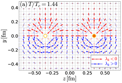
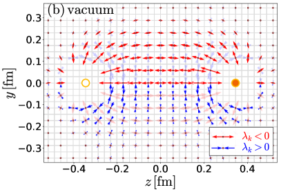
Figure 1: (a) Distribution of the principal axes of ${\cal T}_{ij}$ for a singlet $Q\bar{Q}$ system separated by $R=0.69$ fm in SU(3) Yang-Mills theory with $a=0.038$ fm and $t/a^{2}=2.0$ at $T/T_{c}=1.44$. (b) Distribution of the principal axes of ${\cal T}_{ij}$ in vacuum, where $a=0.029$ fm and $t/a^{2}=2.0$ [1]. In both panels, the red (blue) arrows in the upper (lower) half plane are highlighted. Note that the lengths of arrrows are suitably scaled.

4 Stress Distribution on the Plane including Two Sources

In this section, we consider the stress distribution in the singlet $Q\bar{Q}$ system, focusing first on the plane including two sources. Shown in Fig. 1 (a) is the two eigenvectors of the local stress tensor at $T/T_{c}=1.44$ around the two sources separated by $R=0.69\ {\rm fm}$ obtained on the lattice with $a=0.038\ {\rm fm}$ with fixed $t/{a}^{2}=2.0$. The other eigenvector is perpendicular to this plane. The eigenvector with negative (positive) eigenvalue is denoted by the red outward (blue inward) arrow with its length proportional to $\sqrt{|\lambda_{k}|}$:

$${\color[rgb]{1,0,0}\leftarrow}{\tiny{\circ}}{\color[rgb]{1,0,0}\rightarrow}:\lambda_{k}<0,\qquad{\color[rgb]{0,0,1}\rightarrow}{\tiny{\circ}}{\color[rgb]{0,0,1}\leftarrow}:\lambda_{k}>0.$$ (5)

Neighbouring volume elements are pulling (pushing) with each other along the direction of red (blue) arrow. The arrows in the spatial regions near $Q$ and $\bar{Q}$ , which would suffer from the over-smearing of the gradient flow due to the overlap between the source charge, are excluded. In Fig. 1 (b), we show the stress distribution around $Q\bar{Q}$ in vacuum with the same $Q\bar{Q}$ distance $R=0.69\ {\rm fm}$ obtained in Ref. [1] as a comparison. Fig. 1 (b) clearly reveals the formation of the flux tube in terms of the stress tensor in a gauge invariant manner; the region where the strong stress acts concentrates around the one-dimensional tube structure between $Q\bar{Q}$. On the other hand, Fig. 1 (a) shows that the flux tube, which is formed in vacuum, is dissociated at $T/T_{c}=1.44$ due to medium effects, and the stress distribution around each source behave alomost independently.

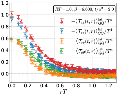
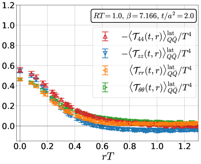
Figure 2: EMT distribution on the mid-plane $-\langle{\cal T}_{44}(t,r)\rangle^{\mathrm{lat}}_{Q\bar{Q}}$ and $-\langle{\cal T}_{cc}(t,r)\rangle^{\mathrm{lat}}_{Q\bar{Q}}$ in the cylindrical coordinate system at $T/T_{c}=1.44\,(\mathrm{left}),2.97\,(\mathrm{right})$ with $RT=1.0$. Note that the lattice spacing and the flow time are fixed.

5 Stress Distribution on the Mid-Plane between Two Sources

Next we focus on the mid-plane between $Q$ and $\bar{Q}$. We use the cylindrical coordinate system $c=(r,\theta,z)$ with $r=\sqrt{x^{2}+y^{2}}$ and $0\leq\theta<2\pi$. On the mid-plane, because of the cylindrical symmetry and the parity symmetry with regard to $z$ axis, the stress tensor is diagonalized as $\langle{\cal T}_{cc^{\prime}}(t,x)\rangle_{Q\bar{Q}}^{\rm lat}={\rm diag}(\langle{\cal T}_{rr}(t,r)\rangle_{Q\bar{Q}}^{\rm lat},\langle{\cal T}_{\theta\theta}(t,r)\rangle_{Q\bar{Q}}^{\rm lat},\langle{\cal T}_{zz}(t,r)\rangle_{Q\bar{Q}}^{\rm lat})$.

In Fig. 2, we show the $r$ dependence of the resulting EMT at $T/T_{c}=1.44$ and $2.97$ with $RT=1.0$ in the normalization $\langle{\cal T}_{cc^{\prime}}(t,x)\rangle_{Q\bar{Q}}^{\rm lat}/T^{4}$. The $Q\bar{Q}$ distance of the left panel in the physical units is $R=0.69$ fm. Note that we fix $t/a^{2}=2.0$ and the lattice spacing $a$ in Fig. 2 and the extrapolation to $(a,t)\to(0,0)$ is not taken. We notice that the thermal expectation value $\langle{\cal T}_{\mu\nu}(t,x)\rangle$ is subtracted in these results so that $\langle{\cal T}_{cc^{\prime}}(t,r\rightarrow\infty)\rangle_{Q\bar{Q}}^{\rm lat}=0$.

From the figure and the comparison with the results in Ref. [1], one finds several noticeable features:

1. Compared with the vacuum result obtained in Ref. [1], the absolute values of all components in the left panel are suppressed in physical units. This suppression is interpreted from the dissociation of the flux tube observed in Fig. 1.
   

2. In the left panel of Fig. 2, there are approximate degeneracies, $\langle{\cal T}_{44}(t,r)\rangle^{\rm lat}_{Q\bar{Q}}\simeq\langle{\cal T}_{zz}(t,r)\rangle^{\rm lat}_{Q\bar{Q}}<0$ and $\langle{\cal T}_{rr}(t,r)\rangle^{\rm lat}_{Q\bar{Q}}\simeq\langle{\cal T}_{\theta\theta}(t,r)\rangle^{\rm lat}_{Q\bar{Q}}>0$, for a wide range of $r$ at $T/T_{c}=1.44$. Also, one sees a separation between these two degenerated channels. From this result, we find $\langle{\cal T}_{\mu\mu}(t,r)\rangle^{\mathrm{lat}}_{Q\bar{Q}}=\langle{\cal T}_{44}(t,r)+{\cal T}_{zz}(t,r)+{\cal T}_{rr}(t,r)+{\cal T}_{\theta\theta}(t,r)\rangle^{\mathrm{lat}}_{Q\bar{Q}}<0$. These features are also found in the stress distribution in vacuum [1].
   

3. By comparing both panels in Fig. 2, one sees that all components tend to be degenerated in the normalization $\langle{\cal T}_{cc^{\prime}}(t,x)\rangle_{Q\bar{Q}}^{\rm lat}/T^{4}$ as $T$ becomes larger. This tendency is in part attributed to the fact that the value of $R=1.0/T$ for $T/T_{c}=2.97$ in physical units is smaller than that for $T/T_{c}=1.44$. As $R$ becomes smaller, the system is dominated by the physics at high-energy scale and the behavior of the EMT around $Q\bar{Q}$ approaches the one described by the leading order in perturbation theory at which all components of the EMT degenerate.

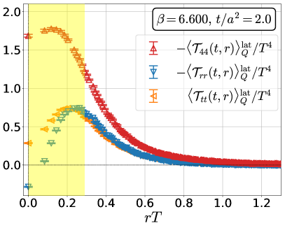
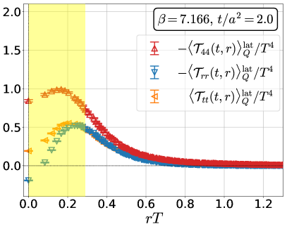
Figure 3: EMT distribution around a single static quark $-\langle{\cal T}_{cc}(t,r)\rangle^{\mathrm{lat}}_{Q}$ and $-\langle{\cal T}_{44}(t,r)\rangle^{\mathrm{lat}}_{Q}$ in the spherical coordinate system at $T/T_{c}=1.44\,(\mathrm{left}),2.97\,(\mathrm{right})$. Note that the lattice spacing and the flow time are fixed. The range of $r$ highlighted by the yellow shades in both figures represents the over-smearing region.

6 Stress Distribution around Single Quark

Finally we consider the single quark system. We employ the spherical coordinate system $c=(r,\theta,\varphi)$ with the radial corrdinate is $r=\sqrt{x^{2}+y^{2}+z^{2}}$ and the polar and azimuthal angles $\theta$ and $\varphi$. The spherical symmetry makes the stress tensor diagonalized as $\langle{\cal T}_{cc^{\prime}}(t,x)\rangle_{Q}^{\rm lat}={\rm diag}(\langle{\cal T}_{rr}(t,r)\rangle_{Q}^{\rm lat},$ $\langle{\cal T}_{tt}(t,r)\rangle_{Q}^{\rm lat},\langle{\cal T}_{tt}(t,r)\rangle_{Q}^{\rm lat})$, where the transverse components $\langle{\cal T}_{tt}(t,r)\rangle_{Q}^{\rm lat}$ are degenerated owing to the rotational symmetry. Shown in Fig. 3 is the profile of each component $\langle{\cal T}_{cc^{\prime}}(t,x)\rangle_{Q}^{\rm lat}$ as a function of $r$ at $T/T_{c}=1.44$ and $2.97$. The yellow shades in Fig. 3 qualitatively represent the range of $r$ which suffers from the overlap between the EMT operator and the Polyakov loop; in this range of $r$, the validity of our analysis is completely lost.

From Fig. 3, one finds an approximate degeneracy of the absolute values of the spatial components $\langle{\cal T}_{rr}(t,r)\rangle_{Q}^{\rm lat}$ and $\langle{\cal T}_{tt}(t,r)\rangle_{Q}^{\rm lat}$. The figure also shows that energy densiy $-\langle{\cal T}_{44}(t,r)\rangle_{Q}^{\rm lat}$ has a clear separation from these channels. One also finds that the magnitudes of all the components become smaller as $T$ becomes larger. This behavior is attributed to the EMT at the leading order in perturbation theory given by $\sim\alpha_{s}^{2}(r)/r^{4}$ with the strong coupling constant $\alpha_{s}(r)=g^{2}/(4\pi)$.

From the EMT distribution around a static quark, it is expected that many interesting features of the medium can be extracted. In the large $r$ region, because the color electric field $E$ behaves as $E\sim e^{-m_{D}r}$, where $m_{D}$ is the Debye screening mass, all the components of EMT damp exponentially $e^{-2m_{D}r}$. On the other hand, in the small $r$ region components of EMT behave as $\sim\alpha^{2}_{s}(r)/r^{4}$. From these behaviors of EMT, one can study the values of $m_{D}$ and $\alpha_{s}(r)$. A numerical confirmation of the mechanical conservation law in the spherical coordinates, $\partial_{r}(r^{2}\mathcal{T}_{rr})=r\mathcal{T}_{tt}$, is another interesting subject.

7 Summary and Outlook

In this proceedings, we have explored the spatial distribution of EMT at nonzero temperature in the single quark system as well as in the singlet $Q\bar{Q}$ system in SU(3) lattice gauge theory. The YM gradient flow plays a crucial role to perform these analyses on the lattice. The dissociation of the flux-tube structure in the $Q\bar{Q}$ system at high temperature in the deconfined phase is observed from the stress distribution.

Although we showed the numerical results with fixed $a$ and $t$ throughout this study, in order to investigate the stress distribution in the continuum limit one has to take the double extrapolation $(a,t)\to(0,0)$. Using the double-extrapolated results, we plan to analyze the static quark systems at nonzero temperature more quantitatively. In particular, the analysis of the Debye screening mass $m_{D}$ and the strong coupling $\alpha_{s}(r)$ from the EMT distribution around a single quark is an interesting future study. There are also a lot of interesting applications of this study, such as the generalization to full QCD with the QCD flow equation [12] and the analyses of the $QQ$ system and the $QQQ$ system at zero and nonzero temperatures.

References

- [1] R. Yanagihara, T. Iritani, M. Kitazawa, M. Asakawa and T. Hatsuda, Phys. Lett. B 789, 210 (2019) doi:10.1016/j.physletb.2018.09.067 [arXiv:1803.05656 [hep-lat]].
- [2] L. D. Landau and E. M. Lifshitz, “ The Classical Theory of Fields” (fourth Edition) (Butterworth-Heinemann, 1980).
- [3] H. Suzuki, PTEP 2013, no. 8, 083B03 (2013) [Erratum: PTEP 2015, no. 7, 079201 (2015)].
- [4] M. Lüscher, JHEP 1008, 071 (2010); M. Lüscher and P. Weisz, JHEP 1102, 051 (2011).
- [5] R. Yanagihara and M. Kitazawa, PTEP 2019, no. 9, 093B02 (2019) doi:10.1093/ptep/ptz093 [arXiv:1905.10056 [hep-ph]].
- [6] Y. Maezawa, T. Umeda, S. Aoki, S. Ejiri , T. Hatsuda, K. Kanaya and H. Ohno, Prog. Theor. Phys. 128, 955 (2012) doi:10.1143/PTP.128.955.
- [7] O. Kaczmarek, F. Karsch, F. Zantow and P. Petreczky, Phys. Rev. D 70, 074505 (2004) Erratum: [Phys. Rev. D 72, 059903 (2005)] doi:10.1103/PhysRevD.70.074505, 10.1103/PhysRevD.72.059903 [hep-lat/0406036].
- [8] R. V. Harlander, Y. Kluth and F. Lange, Eur. Phys. J. C 78, no. 11, 944 (2018) doi:10.1140/epjc/s10052-018-6415-7 [arXiv:1808.09837 [hep-lat]].
- [9] T. Iritani, M. Kitazawa, H. Suzuki and H. Takaura, PTEP 2019, no. 2, 023B02 (2019) doi:10.1093/ptep/ptz001 [arXiv:1812.06444 [hep-lat]].
- [10] M. Kitazawa, T. Iritani, M. Asakawa, T. Hatsuda, and H. Suzuki, Phys. Rev. D 94, 114512 (2016);
- [11] G. Parisi, R. Petronzio, and F. Rapuano, Phys. Lett. 128B, 418 (1983).
- [12] H. Makino and H. Suzuki, PTEP 2014, no. 6, 063B02 (2014) [Erratum: PTEP 2015, no. 7, 079202 (2015)]; Y. Taniguchi, S. Ejiri, R. Iwami, K. Kanaya, M. Kitazawa, H. Suzuki, T. Umeda, and N. Wakabayashi, Phys. Rev. D 96, 014509 (2017).