Backprop Diffusion is Biologically Plausible

Abstract

The Backpropagation algorithm relies on the abstraction of using a neural model that gets rid of the notion of time, since the input is mapped instantaneously to the output. In this paper, we claim that this abstraction of ignoring time, along with the abrupt input changes that occur when feeding the training set, are in fact the reasons why, in some papers, Backprop biological plausibility is regarded as an arguable issue. We show that as soon as a deep feedforward network operates with neurons with time-delayed response, the backprop weight update turns out to be the basic equation of a biologically plausible diffusion process based on forward-backward waves. We also show that such a process very well approximates the gradient for inputs that are not too fast with respect to the depth of the network. These remarks somewhat disclose the diffusion process behind the backprop equation and leads us to interpret the corresponding algorithm as a degeneration of a more general diffusion process that takes place also in neural networks with cyclic connections.

1 Introduction

Backpropagation enjoys the property of being an optimal algorithm for gradient computation, which takes $\Theta(m)$ in a feedforward network with $m$ weights [8, 9]. It is worth mentioning that the gradient computation with classic numerical algorithms would take $O(m^{2})$, which clearly shows the impressive advantage that is gained for nowadays big networks. However, since its conception, Backpropagation has been the target of criticisms concerning its biological plausibility. Stefan Grossberg early pointed out the transport problem that is inherently connected with the algorithm. Basically, for each neuron, the delta error must be “transported” for updating the weights. Hence, the algorithm requires each neuron the availability of a precise knowledge of all of its downstream synapses. Related comments were given by F. Crick [6], who also pointed out that backprop seems to require rapid circulation of the delta error back along axons from the synaptic outputs. Interestingly enough, as discussed in the following, this is consistent with the main result of this paper. A number of studies have suggested solutions to the weight transport problem. Recently, Lillicrap et al [11] have suggested that random synaptic feedback weights can support error backpropagation. However, any interpretation which neglects the role of time might not fully capture the essence of biological plausibility. The intriguing marriage between energy-based models with object functions for supervision that gives rise to Equilibrium Propagation [12] is definitely better suited to capture the role of time. Based the full trust on the role of temporal evolution, in [1], it is pointed out that, like other laws of nature, learning can be formulated under the framework of variational principles.

This paper springs out from recent studies on the problem of learning visual features [3, 4, 2] and it was also stimulated by a nice analysis on the interpretation of Newtonian mechanics equations in the variational framework [10]. It is shown that when shifting from algorithms to laws of learning, one can clearly see the emergence of the biological plausibility of Backprop, an issue that has been controversial since its spectacular impact. We claim that the algorithm does represent a sort of degeneration of a natural spatiotemporal diffusion process that can clearly be understood when thinking of perceptual tasks like speech and vision, where signals possess smooth properties. In those tasks, instead of performing the forward-backward scheme for any frame, one can properly spread the weight update according to a diffusion scheme. While this is quite an obvious remark on parallel computation, the disclosure of the degenerate diffusion scheme behind Backprop, sheds light on its biological plausibility. The learning process that emerges in this framework is based on complex diffusion waves that, however, is dramatically simplified under the feedforward assumption, where the propagation is split into forward and backward waves.

$t$	$t+1$	$t+2$	$t+3$	$t+4$	$t+5$	$t+6$	$t+7$	$t+8$

Figure 1: Forward and backward waves on a ten-level network when the input and the supervision are kept constant. When selecting a certain frame—defined by the time index—the gradient can consistently be computed by Backpropagation on “red-blue neurons”.

2 Backprop diffusion

In this section we consider multilayered networks composed of $L$ layers of neurons, but the results can easily be extended to any feedforward network characterized by an acyclic path of interconnections. The layers are denoted by the index $l$, which ranges from $l=0$ (input layer) to $l=L$ (output layer). Let $W_{l}$ be the layer matrix and $x_{t,l}$ be the vector of the neural output at layer $l$ corresponding to discrete time $t$.

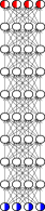
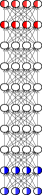
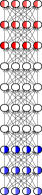
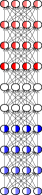
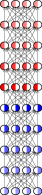
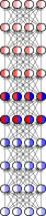
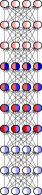
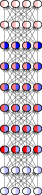
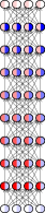
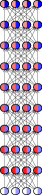
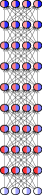
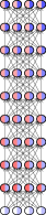
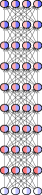
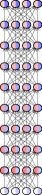
(A) (B) $t$ $t+1$ $t+2$ $t+3$ $t+4$ $t+5$ $t+6$ $t+7$ $t+8$

Figure 2: Forward and backward waves on a ten-level network with slowly varying input and supervision. In (A) it is shown how the input and backward signals fill the neurons; the wavefronts of the waves are clearly visible. Figure (B) instead shows the same diffusion process in stationary conditions when the neurons are already filled up. In this quasi-stationary condition the Backpropagation diffusion algorithm very well approximates the gradient computation. In particular for $l_{s}=(L+1)/2=(9+1)/2=5$ there is a perfect backprop synchronization and the gradient is correctly computed.

$t$	$t+1$	$t+2$	$t+3$	$t+4$	$t+5$	$t+6$	$t+7$	$t+8$

Figure 3: Forward and backward waves on a ten-level network with rapidly changing signal. In this case the Backpropagation diffusion equation does not properly approximate the gradient. However, also in this case, for $l_{s}=5$ we have perfect Backpropagation synchronization with correct syncronization of the gradient.

Here we assume that the network carries out a computation over time, so as, instead of regarding the forward and backward steps as instantaneous processes, we assume that the neuronal outputs follow the time-delay model:

$$x_{t+1,l+1}=\sigma(W_{l}x_{t,l}),$$ (1)

where $\sigma(\cdot)$ is the neural non-linear function. In doing so, when focussing on frame $t$ the following forward process takes place in a deep network of $L$ layers:

$$\left\{\begin{split}x_{t+1,1}&=\sigma(W_{0}x_{t,0})\\ x_{t+2,2}&=\sigma(W_{1}x_{t+1,1})=\sigma(W_{1}\sigma(W_{0}x_{t,0}))\\ &\,\,\,\vdots&\\ x_{t+L,L}&=\sigma(W_{L-1}x_{t,L-1})=\ldots=\sigma(W_{L-1}\sigma(W_{L-2}\ldots\sigma(W_{0}x_{t,0})\ldots)).\end{split}\right.$$ (2)

Hence, the input $x_{t,0}$ is forwarded to layers $1,2,\ldots,L$ a time $t+1,t+2,\ldots,t+L$, respectively, which can be regarded as a forward wave. We can formally state that input $u_{t}:=x_{t,0}$ is forwarded to layer $\kappa$ by the operator $\stackrel{{\scriptstyle\kappa}}{{\rightarrow}}$, that is $\stackrel{{\scriptstyle\kappa}}{{\rightarrow}}u_{t}=x_{t+\kappa,\kappa}$. Likewise, when inspired by the backward step of Backpropagation, we can think of back-propagating the delta error $\delta_{t,L}$ on the output as follows:

$$\left\{\begin{split}\delta_{t+1,L-1}&=\sigma_{L-1}^{\prime}W_{L-1}^{T}\delta_{t,L}\\ \delta_{t+2,L-2}&=\sigma_{L-2}^{\prime}W_{L-2}^{T}\delta_{t+1,L-1}=(\sigma_{L-2}^{\prime}W_{L-2}^{T})\cdot(\sigma_{L-1}^{\prime}W_{L-1}^{T})\cdot\delta_{t,L}\\ &\,\,\,\vdots&\\ \delta_{t+L-1,1}&=\sigma_{1}^{\prime}W_{1}^{T}\delta_{t+L-2,2}=\prod_{\kappa=1}^{L-1}\sigma_{\kappa}^{\prime}W_{\kappa}^{T}\cdot\delta_{t,L}\end{split}\right.$$

Like for $x_{t,l}$, we can formally state that the output delta error $\delta_{t,L}$ is propagated back by the operator $\stackrel{{\scriptstyle L-\kappa}}{{\longleftarrow}}$ defined by $\delta_{t,L}\stackrel{{\scriptstyle\kappa}}{{\longleftarrow}}:=\delta_{t+\kappa,L-\kappa}$. The following equation is still formally coming from Backpropagation, since it represents the classic factorization of forward and backward terms:

$$g_{t,l}=\delta_{t,l}\cdot x_{t,l-1}=\big{(}\stackrel{{\scriptstyle l-1}}{{\longrightarrow}}u_{t-l+1}\big{)}\cdot\big{(}\delta_{t-L+l,L}\stackrel{{\scriptstyle L-l}}{{\longleftarrow}}\big{)}$$ (3)

Clearly, $g_{t,l}$ is the result of a diffusion process that is characterized by the interaction of a forward and of a backward wave (see Fig. 1). This is a truly local spatiotemporal process which is definitely biologically plausible. Notice that if $L$ is odd then for $l_{s}=(L+1)/2$ we have a perfect backprop synchronization between the input and the supervision, since in this case the number of forward steps $l-1$ equals the number of backward steps $L-l$. Clearly, the forward-backward wave synchronization takes place for $L=1$, which is a trivial case in which there is no wave propagation. The next case of perfect synchronization is for $L=3$. In this case, the two hidden layers are involved in one-step of forward-backward propagation. Notice that the perfect synchronization comes with one step delay in the gradient computation. In general, the computation of the gradient in the layer of perfect synchronization is delayed of $l_{s}-1=(L-1)/2$. For all other layers, Eq. 3 turns out to be an approximation of the gradient computation, since the forward and backward waves meet in layers of no perfect synchronization. We can promptly see that, as a matter of fact, synchronization approximatively holds whenever $u_{t}$ is not too fast with respect to $L$ (see Fig. 2 and 3). The maximum mismatch between $l-1$ and $L-l$ is in fact $L-1$, so as if $\Delta t$ is the quantization interval required to perform the computation over a layer, good synchronization requires that $u_{t}$ is nearly constant over intervals of length $\tau_{s}=(L-1)\Delta t$. For example, a video stream, which is sampled at $f_{v}$ frames/sec requires to carry out the computation with time intervals bounded by $\Delta t=\tau_{s}/(L-1)=f_{v}/(L-1)$.

3 Lagrangian interpretation of diffusion on graphs

In the remainder of the paper we show that the forward/backward diffusion of layered networks is just a special case of more general diffusion processes that are at the basis of learning in neural networks characterized by graphs with any pattern of interconnections. In particular we show that this naturally arises when formulating learning as a parsimonious constraint satisfaction problem. We use recent connections established between learning processes and laws of physics under the principle of least cognitive action [1].

Learning	Mechanics	Remarks
$(W,x)$	$u$	Weights and neuronal outputs are interpreted as generalized coordinates.
$(\dot{W},\dot{x})$	$\dot{u}$	Weight variations and neuronal variations are interpreted as generalized velocities.
$\mathscr{A}(x,W)$	$\mathscr{S}(u)$	The cognitive action is the dual of the action in mechanics.

Table 1: Links between learning theory and classical mechanics.

In this paper we make the additional assumption of defining connectionist models of learning in terms of a set of constraints that turn out to be subsidiary conditions of a variational problem [7]. Let us consider the classic example of the feedforward network used to compute the XOR predicate. If we denote with $x^{i}$ the outputs of each neuron and with $w_{ij}$ the weigh associated with the arch $i\mathrel{\!\mathrel{-}\mkern-8.0mu\mathrel{-}\mkern-8.0mu\mathrel{-}\!}j$, then for the neural network in the figure we have $x^{3}=\sigma(w_{31}x^{1}+w_{32}x^{2})$, $x^{4}=\sigma(w_{41}x^{1}+w_{42}x^{2})$ and $x^{5}=\sigma(w_{53}x^{3}+w_{54}x^{4})$. Therefore in the $w-x$ space this compositional relations between the nodes variables can be regarded as constraints, namely $G^{3}=G^{4}=G^{5}=0$, where:

$$G^{3}=x^{3}-\sigma(w_{31}x^{1}+w_{32}x^{2}),\quad G^{4}=x^{4}-\sigma(w_{41}x^{1}+w_{42}x^{2}),$$

$$G^{5}=x^{5}-\sigma(w_{53}x^{3}+w_{54}x^{4}).$$

In addition to these constraints we can also regard the way with which we assign the input values as additional constraints. Suppose we want to compute the value of the network on the input $x^{1}=e^{1}$ and $x^{2}=e^{2}$, where $e^{1}$ and $e^{2}$ are two scalar values; this two assignments can be regarded as two additional constraints $G^{1}=G^{2}=0$ where $G^{1}=x^{1}-e^{1},\quad G^{2}=x^{2}-e^{2}.$ First of all let us describe the architecture of the models that we will address. Given a simple digraph $D=(V,A)$ of order $\nu$, without loss of generality, we can assume $V=\{1,2,\dots,\nu\}$ and $A\subset V\times V$. A neural network constructed on $D$ consists of a set of maps $i\in V\mapsto x^{i}\in{\bf R}$ and $(i,j)\in A\mapsto w_{ij}\in{\bf R}$ together with $\nu$ constraints $G^{j}(x,W)=0$ $j=1,2,\dots\nu$ where $(W)_{ij}=w_{ij}$. Let ${\cal M}_{\nu}({\bf R})$ be the set of all $\nu\times\nu$ real matrices and ${\cal M}^{\downarrow}_{\nu}({\bf R})$ the set of all $\nu\times\nu$ strictly lower triangular matrices over ${\bf R}$. If $W\in{\cal M}^{\downarrow}_{\nu}({\bf R})$ we say that the NN has a feedforward structure. In this paper we will consider both feedforward NN and NN with cycles. The relations $G^{j}=0$ for $j=1,\dots,\nu$ specify the computational scheme with which the information diffuses trough the network. In a typical network with $\omega$ inputs these constraints are defined as follows: For any vector $\xi\in{\bf R}^{\nu}$, for any matrix $M\in{\cal M}_{\nu}({\bf R})$ with entries $m_{ij}$ and for any given ${\cal C}^{1}$ map $e\colon(0,+\infty)\to{\bf R}^{\omega}$ we define the constraint on neuron $j$ when the example $e(\tau)$ is presented to the network as

$$G^{j}(\tau,\xi,M):=\begin{cases}\xi^{j}-e^{j}(\tau),&\text{if $1\leq j\leq\omega$};\\ \xi^{j}-\sigma(m_{jk}\xi^{k})&\text{if $\omega<j\leq\nu$},\end{cases}$$ (4)

where $\sigma\colon{\bf R}\to{\bf R}$ is of class ${\cal C}^{2}({\bf R})$. Notice that the dependence of the constraints on $\tau$ reflects the fact that the computations of a neural network should be based on external inputs.

Principle of Least Cognitive Action

Like in the case of classical mechanics, when dealing with learning processes, we are interested in the temporal dynamics of the variables exposed to the data from which the learning is supposed to happen. Depending on the structure of the matrix $M$, it is useful to distinguish between feedforward networks and networks with loops (recurrent neural networks). Let us therefore consider the functional

$$\mathscr{A}(x,W):=\int{1\over 2}(m_{x}|\dot{x}(t)|^{2}+m_{W}|\dot{W}(t)|^{2})\,\varpi(t)dt+\mathscr{F}(x,W),$$ (5)

with $\mathscr{F}(x,W):=\int F(t,x,\dot{x},\ddot{x},W,\dot{W},\ddot{W})\,dt$ and $t\mapsto\varpi(t)$ a positive continuously differentiable function, subject to the constraints

$$G^{j}(t,x(t),W(t))=0,\qquad 1\leq j\leq\nu,$$ (6)

where the map $G(\cdot,\cdot,\cdot)$ is taken as in Eq. (4). Let $({G_{\xi}\atop\overline{G_{M}}})$ be the Jacobian matrix of the constraints $G$ with respect to $x$ and $W$, where it is intended that the first $\nu$ rows contain the gradients of $G$ with respect to its second argument:

$$\left({G_{\xi}\atop\overline{G_{M}}}\right)_{ij}\equiv G^{j}_{\xi^{i}},\quad\hbox{for $1\leq i\leq\nu$}.$$

Variational problems with subsidiary conditions can be tackled using the method of Lagrange multipliers to convert the constrained problem into an unconstrained one [7]). In order to use this method it is necessary to verify an independence hypothesis between the constraints; in this case we need to check that the matrix $({G_{\xi}\atop\overline{G_{M}}})$ is full rank. Interestingly, the following proposition holds true:

Proposition 1.

The matrix $({G_{\xi}\atop\overline{G_{M}}})\in{\cal M}_{(\nu^{2}+\nu)\times\nu}({\bf R})$ is full rank.

Proof.

First of all notice that if $(G_{\xi})_{ij}=G^{j}_{\xi^{i}}$ is full rank also $({G_{\xi}\atop\overline{G_{M}}})$ has this property. Then, since

$$G^{j}_{\xi^{i}}(\tau,\xi,M)=\begin{cases}\delta_{ij},&\text{if $1\leq j\leq\omega$};\\ \delta_{ij}-\sigma^{\prime}(m_{jk}\xi^{k})m_{ji}&\text{if $\omega<j\leq\nu$,}\end{cases}$$

we immediately notice that $G^{i}_{\xi^{i}}=1$ and that for all $i>j$ we have $G^{i}_{\xi^{i}}=0$. This means that

$$(G^{j}_{\xi^{i}}(\tau,\xi,M))=\begin{pmatrix}1&*&\cdots&*\\ 0&1&\cdots&*\\ \vdots&\vdots&\ddots&\vdots\\ 0&0&\cdots&1\end{pmatrix},$$

which is clearly full rank. ∎

Notice that this result heavily depends on the assumption $W\in{\cal M}^{\downarrow}_{\nu}({\bf R})$ (triangular matrix), which corresponds to feedforward architectures.

Derivation of the Lagrangian multipliers—feedforward networks

Following the spirit of the principle of least cognitive action [1], we begin by deriving the constrained Euler-Lagrange (EL) equations associated with the functional (5) under subsidiary conditions (6) that refer to feedforward neural networks. The constrained functional is

$$\mathscr{A}\ ^{*}(x,W)=\int{1\over 2}(m_{x}|\dot{x}(t)|^{2}+m_{W}|\dot{W}(t)|^{2})\varpi(t)-\lambda_{j}(t)G^{j}(t,x(t),W(t))\,dt+\mathscr{F}(x,W),$$ (7)

and its EL-equations thus read

$$-m_{x}\varpi(t)\ddot{x}(t)-m_{x}\dot{\varpi}(t)\dot{x}(t)-\lambda_{j}(t)G^{j}_{\xi}(x(t),W(t))+L^{x}_{F}(x(t),W(t))=0;$$ (8)

$$-m_{W}\varpi(t)\ddot{W}(t)-m_{W}\dot{\varpi}(t)\dot{W}(t)-\lambda_{j}(t)G^{j}_{M}(x(t),W(t))+L^{W}_{F}(x(t),W(t))=0,$$ (9)

where $L_{F}^{x}=F_{x}-d(F_{\dot{x}})/dt+d^{2}(F_{\ddot{x}})/dt^{2}$, $L_{F}^{W}=F_{W}-d(F_{\dot{W}})/dt+d^{2}(F_{\ddot{W}})/dt^{2}$ are the functional derivatives of $F$ with respect to $x$ and $W$ respectively (see [5]). An expression for the Lagrange multipliers is derived by differentiating two times the equations of the architectural constraints with respect to the time and using the obtained expression to substitute the second order terms in the Euler equations, so as we get:

$$\Bigl{(}{G^{i}_{\xi^{a}}G^{j}_{\xi^{a}}\over m_{x}}+{G^{i}_{m_{ab}}G^{j}_{m_{ab}}\over m_{W}}\Bigr{)}\lambda_{j}= \varpi\bigl{(}G^{i}_{\tau\tau}+2(G^{i}_{\tau\xi^{a}}\dot{x}^{a}+G^{i}_{\tau m_{ab}}\dot{w}_{ab}+G^{i}_{\xi^{a}m_{bc}}\dot{x}^{a}\dot{w}_{bc})$$ (10)

$$+G^{i}_{\xi^{a}\xi^{b}}\dot{x}^{a}\dot{x}^{b}+G^{i}_{m_{ab}m_{cd}}\dot{w}_{ab}\dot{w}_{cd}\bigr{)}$$

$$-\dot{\varpi}(\dot{x}^{a}G^{i}_{\xi^{a}}+\dot{w}_{ab}G^{i}_{m_{ab}})+{L^{x^{a}}_{F}G^{i}_{\xi^{a}}\over m_{x}}+{L^{w_{ab}}_{F}G^{i}_{m_{ab}}\over m_{W}},$$

where $G^{i}_{\tau}$, $G^{i}_{\tau\tau}$, $G^{i}_{\xi^{a}}$, $G^{i}_{\xi^{a}\xi^{b}}$, $G^{i}_{m_{ab}}$ and $G^{i}_{m_{ab}m_{cd}}$ are the gradients and the hessians of constraint (6).

Suppose now that we want to solve Eq.  (8)–(9) with Cauchy initial conditions. Of course we must choose $W(0)$ and $x(0)$ such that $g_{i}(0)\equiv 0$, where we posed $g_{i}(t):=G^{i}(t,x(t),W(t))$, for $i=1,\dots,\nu$. However since the constraint must hold also for all $t\geq 0$ we must also have at least $g^{\prime}_{i}(0)=0$. These conditions written explicitly means

$$G^{i}_{\tau}(0,x(0),W(0))+G^{i}_{\xi^{a}}(0,x(0),W(0))\dot{x}^{a}(0)+G^{i}_{m_{ab}}(0,x(0),W(0))\dot{w}_{ab}(0)=0.$$

If the constraints does not depend explicitly on time it is sufficient to to choose $\dot{x}(0)=0$ and $\dot{W}(0)=0$, while for time dependent constraint this condition leaves

$$G^{i}_{\tau}(0,x(0),W(0))=0,$$

which is an additional constraint on the initial conditions $x(0)$ and $W(0)$ to be satisfied. Therefore one possible consistent way to impose Cauchy conditions is

$$G^{i}(0,x(0),W(0))=0,\quad i=1,\dots,\nu;$$ (11)

$$G^{i}_{\tau}(0,x(0),W(0))=0,\quad i=1,\dots,\nu;$$

$$\dot{x}(0)=0;$$

$$\dot{W}(0)=0.$$

Reduction to Backpropagation

To understand the behaviour of the Euler equations (8) and (9) we observe that in the case of feedforward networks, as it is well known, the constraints $G^{j}(t,x,W)=0$ can be solved for $x$ so that eventually we can express the value of the output neurons in terms of the value of the input neurons. If we let $f^{i}_{W}(e(t))$ be the value of $x^{\nu-i}$ when $x^{1}=e^{1}(t),\dots,x^{\omega}=e^{\omega}(t)$, then the theory defined by (5) under subsidiary conditions (6) is equivalent, when $m_{x}=0$ and $\varpi(t)=\exp(\vartheta t)$, to the unconstrained theory defined by

$$\int e^{\vartheta t}\Bigl{(}\frac{m_{W}}{2}|\dot{W}|^{2}-\overline{V}(t,W(t))\Bigr{)}\,dt$$ (12)

where $\overline{V}$ is a loss function for which a possible choice is $\overline{V}(t,W(t)):=\frac{1}{2}\sum_{i=1}^{\eta}(y^{i}(t)-f^{i}_{W}(E(t)))^{2}$ with $y(t)$ an assigned target. The Euler equations associated with (12) are

$$\ddot{W}(t)+\vartheta\dot{W}(t)=-\frac{1}{m_{W}}\overline{V}_{W}(t,W(t)),$$ (13)

that in the limit $\vartheta\to\infty$ and $\vartheta m\to\gamma$ reduces to the gradient method

$$\dot{W}(t)=-\frac{1}{\gamma}\overline{V}_{W}(t,W(t)),$$ (14)

with learning rate $1/\gamma$. Notice that the presence of the term $\varpi(t)$ that we proposed in the general theory it is essential in order to have a learning behaviour as it responsible of the dissipative behaviour.

Typically the term $\overline{V}_{W}(t,W(t))$ in Eq. (14) can be evaluated using the Backpropagation algorithm; we will now show that Eq. (8)–(10) in the limit $m_{x}\to 0$, $m_{W}\to 0$, $m_{x}/m_{W}\to 0$ reproduces Eq. (14) where the term $\overline{V}_{W}(t,W(t))$ explicitly assumes the form prescribed by BP. In order to see this choose $\vartheta=\gamma/m_{W}$, $\varpi(t)=\exp(\vartheta t)$,

$$F(t,x(t),\dot{x}(t),\ddot{x}(t),W(t),\dot{W}(t),\ddot{W}(t))=-e^{\vartheta t}V(t,x(t)),$$

and multiply both sides of Eq. (8)–(10) by $\exp(-\vartheta t)$; then take the limit $m_{x}\to 0$, $m_{W}\to 0$, $m_{x}/m_{W}\to 0$. In this limit Eq. (9) and Eq. (10) becomes respectively

$$\dot{W}_{ij}=-\frac{1}{\gamma}\sigma^{\prime}(w_{ik}x^{k})\delta_{i}x^{j};$$ (15)

$$G^{i}_{\xi^{a}}G^{j}_{\xi^{a}}\delta_{j}=-V_{x^{a}}G^{i}_{\xi^{a}},$$ (16)

where $\delta_{j}$ is the limit of $\exp(-\vartheta t)\lambda_{j}$. Because the matrix $G^{i}_{\xi^{a}}$ is invertible Eq. (16) yields

$$T\delta=-V_{x},$$ (17)

where $T_{ij}:=G^{j}_{\xi^{i}}$. This matrix is an upper triangular matrix thus showing explicitly the backward structure of the propagation of the delta error of the Backpropagation algorithm. Indeed in Eq. (15) the Lagrange multiplier $\delta$ plays the role of the delta error.

In order to better understand the perfect reduction of our approach to the backprop algorithm consider the following example. We simply consider a feedforward network with an input, an output and an hidden neuron. In this case the matrix $T$ is

$$T=\begin{pmatrix}1&-\sigma^{\prime}(w_{21}x^{1})w_{21}&0\\ 0&1&-\sigma^{\prime}(w_{32}x^{2})w_{32}\\ 0&0&1\end{pmatrix}.$$

Then according to Eq. (17) the Lagrange multipliers are derived as follows $\delta_{3}=-V_{x^{3}},\delta_{2}=\sigma^{\prime}(w_{32}x^{2})w_{32}\delta_{3}$, and $\delta_{1}=\sigma^{\prime}(w_{21}x^{1})w_{21}\delta_{2}$. This is exactly the Backpropagation formulas for the delta error. Notice that in this theory we also have an expression for the multipliers of the input neurons, even though, in this case, they are not used to update the weights (see Eq. (15)).

Diffusion on cyclic graphs

The constraint-based analysis carried out so far assumes holonomic constraints, whereas the claim of this paper is that we cannot neglect temporal dependencies, which leads to expressing neural models by non-holonomic constraints. In doing so, we go beyond the constraints expressed by Eq. (6) which imply an infinite velocity of diffusion of information. Since we are stressing the importance of time in learning processes, it is natural to assume that the velocity of information diffusion through a network is finite. In the discrete setting of computation this is reflected by the model 1 discussed in Section 2. A simple classic translation of this constraint in continuous time is

$$c^{-1}\dot{x}^{i}(t)=-x^{i}(t)+\sigma(w_{ik}(t)x^{k}(t)),$$ (18)

where $c>0$ can be interpreted as a “diffusion speed”. In stationary situation indeed Eq. (18) coincide with the usual neuron equation in Eq. (6). However, we are in front of a much more complicated constraint, since not only it involves the variables $x$ and $w$, but also their derivatives. Such constraints are called non-holonomic constraints. Now we snow show how to determine the stationarity conditions of the functional

$$\mathscr{A}(x,W)=\int\left(\frac{m_{x}}{2}|\dot{x}(t)|^{2}+\frac{m_{W}}{2}|\dot{W}(t)|^{2}+F(t,x,W)\right)\,\varpi(t)\,dt$$

under the nonholomic constraints

$$G^{i}(t,x(t),W(t),\dot{x}(t)):=c^{-1}\dot{x}^{i}(t)+x^{i}(t)-\sigma(w_{ik}(t)x^{k}(t))=0,\qquad i=1,\dots,r,$$ (19)

by making use of the rule of the Lagrange multipliers. As usual we consider the stationary points of the functional

$$\begin{split}\mathscr{A}^{*}(x,W)=&\int\left(\frac{m_{x}}{2}|\dot{x}(t)|^{2}+\frac{m_{W}}{2}|\dot{W}(t)|^{2}+F(t,x,W)\right)\,\varpi(t)\,dt\\ &-\int\lambda_{j}(t)G^{j}(t,x(t),W(t),\dot{x}(t))\,dt.\end{split}$$

The Euler equations for $\mathscr{A}^{*}$ are

$$\begin{split}&c^{-1}\dot{x}^{i}(t)+x^{i}(t)-\sigma(w_{ik}(t)x^{k}(t))=0;\\ &-m_{W}\varpi(t)\ddot{W}(t)-m_{W}\dot{\varpi}\dot{W}(t)-\lambda_{j}G^{j}_{M}(t,x(t),W(t),\dot{x}(t))+\varpi(t)F_{W}(t,x(t),W(t))=0;\\ &-m_{x}\varpi(t)\ddot{x}(t)-m_{x}\dot{\varpi}\dot{x}(t)+\dot{\lambda}_{j}G^{j}_{p}(t,x(t),W(t),\dot{x}(t))+\lambda_{j}\frac{d}{dt}G^{j}_{p}(t,x(t),W(t),\dot{x}(t))\\ &\qquad-\lambda_{j}G^{j}_{\xi}(t,x(t),W(t),\dot{x}(t))+\varpi(t)F_{x}(t,x(t),W(t))=0.\end{split}$$

Again, if we assume that $F(t,x,W)=-V(t,x)$, $\varpi(t)=e^{\vartheta t}$, $\delta_{j}=e^{-\vartheta t}\lambda_{j}$ and we explicitly use the expression for $G^{j}_{p}$ we get

$$\begin{split}&c^{-1}\dot{x}^{i}(t)+x^{i}(t)-\sigma(w_{ik}(t)x^{k}(t))=0;\\ &-m_{W}\ddot{W}(t)-m_{W}\vartheta\dot{W}(t)-\delta_{j}G^{j}_{M}(t,x(t),W(t),\dot{x}(t))=0;\\ &-m_{x}\ddot{x}(t)-m_{x}\vartheta\dot{x}(t)+c^{-1}\dot{\delta}-\delta_{j}G^{j}_{\xi}(t,x(t),W(t),\dot{x}(t))-V_{\xi}(t,x(t))=0.\end{split}$$

This systems of equations can be better interpreted in the limit in which we recovered the backprop rule in Section 4; that is to say in the limit $m_{x}\to 0$, $m_{x}\to 0$ and $m_{x}/m_{W}\to 0$, $\theta\to\infty$ and $\theta m_{W}=\gamma$ fixed. Under this conditions, we have the following further reduction

$$\begin{split}&c^{-1}\dot{x}^{i}(t)+x^{i}(t)-\sigma(w_{ik}(t)x^{k}(t))=0;\\ &\dot{W}(t)=-\frac{1}{\gamma}\delta_{j}(t)G^{j}_{M}(t,x(t),W(t),\dot{x}(t));\\ &c^{-1}\dot{\delta}(t)=\delta_{j}(t)G^{j}_{\xi}(t,x(t),W(t),\dot{x}(t))+V_{\xi}(t,x(t)).\end{split}$$ (20)

The equation that defines the Lagrange multipliers $\delta$ is now a differential equation that explicitly gives us the correct updating rule instead of a instantaneous equation that must be solved for each $t$. As the diffusion speed becomes infinite ($c\to+\infty$) Eq. (20) reproduce Backpropagation, which is consistent with the intuitive explanation that arises from Fig. 1, 2, 3.

4 Conclusions

In this paper we have shown that the longstanding debate on the biological plausibility of Backpropagation can simply be addressed by distinguishing the forward-backward local diffusion process for weight updating with respect to the algorithmic gradient computation over all the net, which requires the transport of the delta error through the entire graph. Basically, the algorithm expresses the degeneration of a biologically plausible diffusion process, which comes from the assumption of a static neural model. The main conclusion is that, more than Backpropation, the appropriate target of the mentioned longstanding biological plausibility issues is the assumption of an instantaneous map from the input to the output. The forward-backward wave propagation behind Backpropagation, which is in fact at the basis of the corresponding algorithm, is proven to be local and definitely biologically plausible. This paper has shown that an opportune embedding in time of deep networks leads to a natural interpretation of Backprop as a diffusion process which is fully local in space and time. The given analysis on any graph-based neural architectures suggests that spatiotemporal diffusion takes place according to the interactions of forward and backward waves, which arise from the environmental interaction. While the forward wave is generated by the input, the backward wave arises from the output; the special way in which they interact for classic feedforward network corresponds to the degeneration of this diffusion process which takes place at infinite velocity. However, apart from this theoretical limit, Backpropagation diffusion is a truly local process.

Broader Impact

Our work is a foundational study. We believe that there are neither ethical aspects nor future societal consequences that should be discussed.

References

- [1] Alessandro Betti and Marco Gori. The principle of least cognitive action. Theor. Comput. Sci., 633:83–99, 2016.
- [2] Alessandro Betti and Marco Gori. Convolutional networks in visual environments. CoRR, abs/1801.07110, 2018.
- [3] Alessandro Betti, Marco Gori, and Stefano Melacci. Cognitive action laws: The case of visual features. IEEE transactions on neural networks and learning systems, 2019.
- [4] Alessandro Betti, Marco Gori, and Stefano Melacci. Motion invariance in visual environments. In Proceedings of the Twenty-Eighth International Joint Conference on Artificial Intelligence, IJCAI-19, pages 2009–2015. International Joint Conferences on Artificial Intelligence Organization, 7 2019.
- [5] R Courant and D Hilbert. Methods of Mathematical Physics, volume 1, page 190. Interscience Publ., New York and London, 1962.
- [6] Francis Crick. The recent excitement about neural networks. Nature, 337:129–132, 1989.
- [7] M. Giaquinta and S. Hildebrand. Calculus of Variations I, volume 1. Springer, 1996.
- [8] Ian Goodfellow, Yoshua Bengio, and Aaron Courville. Deep Learning. The MIT Press, 2016.
- [9] Marco Gori. Machine Learning: A Constrained-Based Approach. Morgan Kauffman, 2018.
- [10] Matthias Liero and Ulisse Stefanelli. A new minimum principle for lagrangian mechanics. Journal of Nonlinear Science, 23:179–204, 2013.
- [11] T.P. Lillicrap, D. Cownden, D.B. Twed, and C.J. Akerman. Random synaptic feedback weights support error backpropagation for deep learning. Nature Communications, Jan 2016.
- [12] Benjamin Scellier and Yoshua Bengio. Equivalence of equilibrium propagation and recurrent backpropagation. Neural Computation, 31(2), 2019.