Quench dynamics of entanglement spectra and topological superconducting phases in a long-range Hamiltonian

Abstract

We study the quench dynamics of entanglement spectra in the Kitaev chain with variable-range pairing quantified by power-law decay rate $\alpha$. Considering the post-quench Hamiltonians with flat bands, we demonstrate that the presence of entanglement-spectrum crossings during its dynamics is able to characterize the topological phase transitions (TPTs) in both short-range ($\alpha>1$) and long-range ($\alpha<1$) sectors. Novel properties of entanglement-spectrum dynamics are revealed for the quench protocols in the long-range sector or with $\alpha$ as the quench parameter. In particular, when the lowest upper-half entanglement-spectrum value of initial Hamiltonian is smaller than the final one, the TPTs can also be diagnosed by the difference between the lowest two upper-half entanglement-spectrum values if the half-way winding number is not equal to that of the initial Hamiltonian. Moreover, we discuss the stability of characterizing the TPTs via entanglement-spectrum crossings against energy dispersion in the long-range model.

I Introduction

Topological superconductors have attracted considerable interests in recent years. The Majorana zero modes in those systems, being robust against disorder Qi and Zhang (2011); Sato and Ando (2017); Nadj-Perge et al. (2014); Mourik et al. (2012), play a key role in the realization of topological quantum computation Sarma et al. (2015); Mong et al. (2014); Kraus et al. (2013); Alicea (2012); Kitaev (2003). One of the most intriguing topological superconductors is the Kitaev chain with long-range $p$-wave pairing terms, where novel topological phases with fractional winding numbers and massive Dirac edge states are found Viyuela et al. (2016). More importantly, the Hamiltonian can be realized in magnetic atomic chains Nadj-Perge et al. (2014); Choi et al. (2017); Ménard et al. (2017, 2015) with the long-range pairing induced by magnetic impurities Neupert et al. (2016); Pientka et al. (2014); Klinovaja et al. (2013); Nadj-Perge et al. (2013); Pientka et al. (2013); Kaladzhyan et al. (2016); Heinrich et al. (2018).

The characterization of topological phase transitions (TPTs), beyond the Laudau symmetry-breaking paradigm, is also of great significance. From the perspective of quantum information, it has been shown that the quantum coherence Li and Sun (2018); Qiao et al. (2019), multipartite entanglement Pezzè et al. (2017); Zhang et al. (2018a); Gabbrielli et al. (2018); Yin et al. (2019), entanglement entropy Kitaev and Preskill (2006); Levin and Wen (2006); Vodola et al. (2014); Fromholz et al. (2019) and entanglement spectrum Li and Haldane (2008); Pollmann et al. (2010); Fidkowski (2010) of the ground state can detect the TPTs. Recently, the rapid developments of quantum simulation based on ultracold atoms Gross and Bloch (2017); Fläschner et al. (2018); Sun et al. (2018), trapped ions Blatt and Roos (2012) and superconducting qubits Neill et al. (2017); Yan et al. (2019) have stimulated the study of quench dynamics. It is therefore natural to extend the characterization of TPTs to an out-of-equilibrium regime Wilson et al. (2016); Wang et al. (2017); Maffei et al. (2018); Zhang et al. (2018b); Potter et al. (2016). For instance, the quench dynamics of entanglement spectra in the topological insulators and superconductors with nearest-neighbor terms, involving the standard Su-Schrieffer-Heeger model Su et al. (1979) and Kitaev chain Kitaev (2001) are studied, suggesting its close relationship with TPTs Gong and Ueda (2018); Chang (2018); Lu and Yu (2019). Nevertheless, the investigation of the entanglement-spectrum non-equilibrium behaviors in long-range models remains limited, and the methods useful in short-range systems can be further generalized.

In this work, we explore the quench dynamics of entanglement spectra in the Kitaev chain with long-range pairing, whose topological phase diagram is more complex than the previously studied models Viyuela et al. (2016); Vodola et al. (2014). The values of entanglement spectra can be efficiently measured via the quantum state tomography implemented in various artificially-engineered platforms Xu et al. (2018); Lanyon et al. (2018); Choo et al. (2018). Therefore, our results can be tested by state-of-art quantum simulation experiments. The remainder is organized as follows. In Sec. II, we briefly review the Hamiltonian and the topological phases of this model, and the definition of the single-particle entanglement spectrum. We also calculate the lowest upper-half entanglement-spectrum value of ground state in this model and present a physical picture of our work. In the following, the lowest one refers to the lowest upper-half one, the meaning of which will be explained in Sec. II. B. In Sec. III, we study the quench dynamics of entanglement spectra in the Kitaev chain with variable range pairing, revealing several novel nonequilibrium properties of entanglement spectra and demonstrating that the TPTs in the long-range Hamiltonian can be characterized by the quench dynamics of entanglement spectra. In Sec. IV, we conclude and provide some outlooks.

II Preliminary

II.1 The model

We focus on the long-range Kitaev chain with power-law decay pairing terms Viyuela et al. (2016); Vodola et al. (2014), as a generalization of the standard Kitaev chain with only nearest-neighbor terms Kitaev (2001). The Hamiltonian reads

$$H= - \frac{t}{2}\sum_{i=1}^{N}(c_{i}^{\dagger}c_{i+1}+\text{H.c.})-\mu\sum_{i=1}^{N}(c_{i}^{\dagger}c_{i}-\frac{1}{2})$$ (1)

$$+ \frac{\Delta}{2}\sum_{i=1}^{N}\sum_{l=1}^{N-i}\frac{1}{d_{l}^{\alpha}}(c_{i}c_{i+l}+\text{H.c.}),$$

where $c_{i}$ ($c_{i}^{\dagger}$) denotes the annihilation (creation) fermion operator at each site $i$, $N$ is the length of Kitaev chain, and $t$ and $\mu$ represent the hopping amplitude and the chemical potential, respectively. The amplitude of pairing $\Delta$ decay with the parameter $\alpha$ (the decay rate) of the distance $d_{l}$. Here, the antiperiodic boundary condition $c_{i+N}=-c_{i}$ (see Appendix A for the reason behind the choice of the antiperiodic boundary condition), and the condition of closed chain, i.e., $d_{l}=l$ for $l\in[1,N/2]$, while $d_{l}=N-l$ for $l\in[N/2,N]$, are adopted.

By switching to the momentum space via the Fourier transformation, the Hamiltonian (1) can be written as $H=\sum_{k}\epsilon_{k}\Psi_{k}^{\dagger}(\bm{d}_{k}\cdot\bm{\sigma})\Psi_{k}$ with $\Psi_{k}^{\dagger}$ as the Nambu spinor and $\bm{\sigma}$ as the Pauli vector. The winding vector is

$$\bm{d}_{k} = (d_{k}^{x},d_{k}^{y},d_{k}^{z})$$ (2)

$$= (0,-\frac{1}{2}\Delta f_{\alpha}(k),-\frac{\mu+t\cos k}{2})$$

where $k=(2\pi/N)(n+1/2)$ $(n=0,1,...,N-1)$ and $f_{\alpha}(k)=\sum_{i=1}^{N-1}\sin(kl)/d_{l}^{\alpha}$. The energy spectra is then $\epsilon_{k}=|\bm{d}_{k}|$. The topological phases in this model can be characterized by the Z topological invariant winding number Chiu et al. (2016) defined as

$$w=\frac{1}{2\pi}\oint dk\left(\frac{\partial_{k}d_{k}^{z}}{d_{k}^{y}}\right),$$ (3)

which can be rewritten as $w=(1/2\pi)\oint(ydz-zdy)/|\bm{d}_{k}|^{2}$ with $y$ ($z$) as the $y$ $(z)-$component of Eq. (2). Intuitively, it counts how many times $\bm{d}_{k}$ loops around the origin in the $y-z$ plane. Thus, the winding number can also be obtained by simply plotting the trajectory of the winding vector Eq. (2). The phase diagram of the Hamiltonian (1) with $t=-\Delta=1$ (which is fixed in the rest of this work) is shown in Fig. 1(a). The topological phases are similar to the Kitaev chain with the nearest pairing term in the short-range sector ($\alpha>1$), while different from the conventional Kitaev chain in the long-range sector ($\alpha<1$). In particular, the topological phase with a massive Dirac edge mode has winding number $1/2$, however the winding number of the trivial phase is $-1/2$.

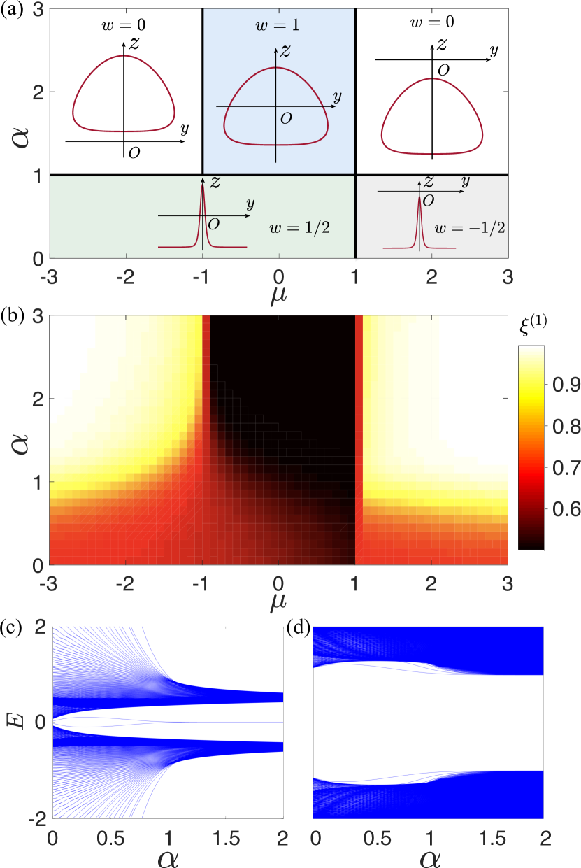
Figure 1: (a) Phase diagram of the Hamiltonian (1) with $t=-\Delta=1$, characterized by the winding number and the trajectory of $\bm{d}_{k}$. (b) The lowest entanglement-spectrum value $\xi^{(1)}$ for the ground state of Hamiltonian (1) with $t=-\Delta=1$ as a function of $\alpha$ and $\mu$. (c) The energy spectra for the Hamiltonian (1) with $t=-\Delta=1$ and $\mu=0$ as a function of $\alpha$. (d) is similar to (c) but with $\mu=-3$. Here, the system size is $N=200$. We emphasize that the depicted energy spectra are obtained by directly diagonalizing the Hamiltonian with open boundary conditions.

Our quench protocol is as follows: The initial state is prepared as the ground state of a Hamiltonian $H^{i}$ (the initial Hamiltonian). We then evolve it with the final Hamiltonian $H^{f}$. Notice that the evolved state can be viewed as the ground state of the following Hamiltonian

$$H(t)=e^{-iH^{f}t}H^{i}e^{iH^{f}t}$$ (4)

In the momentum space, this Hamiltonian can be similarly represented by its winding vector, whose dynamics reads Gong and Ueda (2018)

$$\partial_{t}\bm{d}_{k}(t)=2\bm{d}^{f}_{k}\times\bm{d}_{k}(t),$$ (5)

which can be explicitly solved as

$$\bm{d}_{k}(t)= [ 1-\cos(2|\bm{d}_{k}^{f}|t)][\bm{d}^{i}_{k}\cdot\bm{n}_{k}^{f}]\bm{n}_{k}^{f}$$ (6)

$$+ \cos(2|\bm{d}_{k}^{f}|t)\bm{d}_{k}^{i}+\sin(2|\bm{d}_{k}^{f}|t)[\bm{d}_{k}^{i}\times\bm{n}_{k}^{f}]$$

with $\bm{d}_{k}^{i}$ ($\bm{d}_{k}^{f}$) referring to the winding vector of $H^{i}$ ($H^{f}$), and $\bm{n}_{k}^{f}\equiv-\bm{d}_{k}^{f}/|\bm{d}_{k}^{f}|$.

Here, we briefly mention the concept of band flattening. A flat-band Hamiltonian is obtained by a continuous deformation of the original Hamiltonian, setting the eigenvalues as $\pm 1$. The winding vectors of the flat-band Hamiltonian are all of length 1.

II.2 Entanglement spectrum

Next, we present the definition of entanglement spectrum. In a fermionic model, the reduced density matrix of a subsystem $\mathcal{A}$ has the form  Cheong and Henley (2004)

$$\rho_{\mathcal{A}}\propto\exp(-\sum_{q}\Omega_{q}\gamma_{q}^{\dagger}\gamma_{q}),$$ (7)

which is closely related to the single-particle entanglement spectrum defined as Hughes et al. (2011)

$$\xi_{q}\equiv 1/[1+\exp(-\Omega_{q})]$$ (8)

with $\Omega_{q}>0$. The method of calculating the $\Omega_{q}$ for the system Eq. (1) and its dynamics Eq. (4) is presented in Appendix B. In this work, we mainly discuss the first and second lowest entanglement-spectrum value denoted as $\xi^{(1)}$ and $\xi^{(2)}$ respectively.

An exact correspondence between the entanglement spectrum and the spectrum of physical edge modes is given in Ref. Fidkowski (2010). Specifically, entanglement spectrum can be casted into the form

$$\xi_{q}=\frac{1}{2}+\frac{\lambda_{q}}{2}.$$ (9)

In the following, we focus on the single-particle entanglement spectra whose values are larger than $1/2$, i.e., the upper-half ones, since all the spectra come in pair and are related by a particle-hole transformation. The $\lambda_{q}$ equals the energy spectrum of the corresponding spectrally flattened Hamiltonian restricted to subsystem $\mathcal{A}$. Since band-flattening in general does not change the topology of the system, topological edge modes can be directly read off by looking at the low-lying entanglement spectra. As an example, topological superconductors in BDI class is characterized by a Z topological index Kitaev (2009). This topological invariant is directly related to the winding number $w$, and gives the number of massless edge modes on one edge ($\lambda_{q}=0$). In this case, the $\xi^{(1)}$ will be $1/2$, and we refer to this phenomena as the entanglement-spectrum crossing(s).

Before we study the quench dynamics of entanglement spectra, we first illustrate the properties of $\xi^{(1)}$ for the ground states as a benchmark. As shown in Fig. 1(b), in the short-range sector ($\alpha>1$), the topological phase can be characterized by the $\xi^{(1)}$ for the ground states. The $\xi^{(1)}\simeq 0.5$ for the topological phase while $\xi^{(1)}\simeq 1$ in the trivial phase, corresponding to the presence or absence of massless edge modes. This difference is however less prominent in the long-range sector ($\alpha<1$). Since the long range topological phase features a massive edge mode, the $\xi^{(1)}$ in general is not close to 0.5. Nevertheless, we could still pinpoint the phase boundary $\mu_{c}=1$ by the sharp change of $\xi^{(1)}$.

We also plot the energy spectra as a function of $\alpha$ for $\mu=0$ and $\mu=-3$ in Fig. 1(c) and (d) respectively. With $\mu=0$, we observe massive Dirac fermions when $\alpha<1$ and one massless edge state when $\alpha>1$. However, with $\mu=-3$, there is no massless edge state when $\alpha>1$. The results of energy spectrum reveal the mechanism of the TPTs driven by $\alpha$. It can be recognized that at the critical point $\alpha_{c}=1$, there is a gap of the energy spectrum, which can explain that the phase boundary $\alpha_{c}=1$ is less distinguishable, and the change of $\xi^{(1)}$ is continuous when crossing the phase boundary (shown in Fig. 1(b)). In addition, the more obvious phase boundary $\mu_{c}=1$ in the long-range sector also corresponds to the behaviors of energy spectrum. In Ref. Viyuela et al. (2016), it is seen that the energy spectrum of the system becomes gapless at the critical point $\mu_{c}=1$ for both short and long-range sector.

II.3 Physical picture

To focus on the topological properties of the quench dynamics, we can restrict ourselves to the case where $H^{f}$ is a band-flattened Hamiltonian. For concreteness, we can take the length of winding vector $\epsilon_{k}=|\bm{d}_{k}|$ to be 1. With this condition the winding vectors $d_{k}(t)$ will process at the same velocity. The Hamiltonian $H(t)$ is thus time-periodic. It has been shown that for short-range systems, entanglement-spectrum crossings will appear half-way through the time evolution, i.e., $t=\pi/2$, and the number of crossings are related to the dynamical topological indices. Here, we present a physical picture to relate the number of crossings to the topological indices of $H^{i}$ and $H^{f}$. Utilizing this picture, we will then present and analyze most of our results on the long-range Kitaev chains and explain how the entanglement-spectrum behaviors differ from the short-range case.

The topological superconductor considered here belongs to the BDI class, and the winding vectors will lie on the $y-z$ plane due to the symmetry constraints. In our quench protocol, $\bm{d}^{i}$ and $\bm{d}^{f}$ will satisfy this condition, while $\bm{d}(t)$ will not lie in one plane for an arbitrary time instant. The only exception will be $t=\pi/2$ and $t=0(\pi)$, while the latter case is simply $\bm{d}^{i}$ itself. The half-way entanglement-spectrum crossings is then associated with the half-way winding vector, i.e., $\bm{d}(\pi/2)$. Since the $\bm{d}(\pi/2)$ still possesses the symmetry constraints, the number of its edge modes can be directly counted by the winding number. We can then view the half-way entanglement spectra as characterizing the topology of this half-way Hamiltonian.

III Results

III.1 Chemical potential $\mu$ as the quench parameter

We first focus on the entanglement-spectrum dynamical properties with the quench protocols where the chemical potential $\mu$ is chosen as the quench parameter, i.e., $\mu=\mu_{i}\rightarrow\mu_{f}$, and other parameters are fixed. The $\mu_{i}$ and $\mu_{f}$ refer to the chemical potential of the initial and final Hamiltonian respectively.

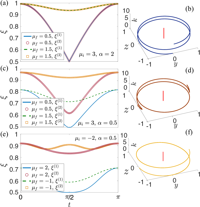
Figure 2: (a) Time evolution of the first and second lowest entanglement-spectrum value $\xi^{(1)}$ and $\xi^{(2)}$ with the quench protocol $\mu=3\rightarrow 1.5$ and $0.5$ in the Hamiltonian (1) with $\alpha=2$ and $\Delta=t=1$. (b) The trajectory of $\bm{d}_{k}$ at time $t=\pi/2$ for the quench protocol in (a) with $\mu_{f}=1.5$. (c) and (d) are similar to (a) and (b), respectively, but with another quench protocol $\mu=3\rightarrow 1.5$ and $0.5$ in the Hamiltonian (1) with $\alpha=0.5$ (e) is similar to (a), but with another quench protocol $\mu=-2\rightarrow-1$ and $2$ in the Hamiltonian (1) with $\alpha=0.5$. (f) is similar to (b) but for the quench protocol in (e) with $\mu_{f}=2$.

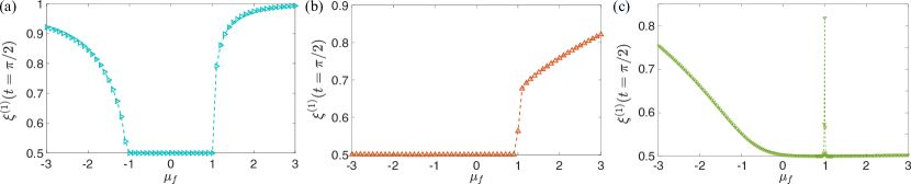
Figure 3: (a) The lowest entanglement-spectrum value for the quench state at $t=\pi/2$, i.e., $\xi^{(1)}(t=\pi/2)$, with the quench protocol $\mu=3\rightarrow\mu_{f}$ as a function of $\mu_{f}$ in the Hamiltonian (1) with $\alpha=2$. Here, the critical points are $\mu_{c}=\pm 1$. (b) is similar to (a) but in the Hamiltonian (1) with $\alpha=0.5$, and the critical point is $\mu_{c}=1$ (c) is similar to (a) but with the quench protocol $\mu=-3\rightarrow\mu_{f}$ in the Hamiltonian (1) with $\alpha=0.5$, and the critical point is $\mu_{c}=1$.

As a warm up, we review the results in the systems with nearest-neighbor interactions. Taking $H^{i}$ to be in the trivial phase, there will always be two degenerate entanglement-spectrum crossings as long as $H^{f}$ belongs to the topological phase. If $H^{f}$ is also in the trivial phase, even the lowest entanglement-spectrum value is far away from 1/2. Thus the entanglement-spectrum crossings provide a distinctive signature for diagnosing topological phases Gong and Ueda (2018); Chang (2018); Lu and Yu (2019). We now show that similar entanglement-spectrum behaviors can also be observed in our Hamitonian (1) in the short-range sector ($\alpha>1$). We study the quench dynamics with the parameters in (1) as $\Delta=t=1$, $\alpha=2$ and $\mu_{i}=3$. The results are depicted in Fig. 2(a). It can be seen that the $\xi^{(1)}$ approaches $0.5$ for $\mu_{f}=1.5$ while it remains a larger value ($>0.9$) for $\mu_{f}=0.5$, characterizing the presence or absence of a TPT. Moreover, the degeneracy of two lowest entanglement-spectrum values, i.e., $\xi^{(1)}=\xi^{(2)}$, is observed for both $\mu_{f}=1.5$ and $0.5$, which can be interpreted by looking at the half-way winding vector. In Fig. 2(b), we plot the trajectory of $\bm{d}_{k}$ at the time $t=\pi/2$, indicating that the winding number of the quenched state is $w=2$, thus explaining the doubly degenerate crossings. It has also been demonstrated that the quench dynamics of entanglement spectra with a nontrivial $H^{i}$, such as one with $w=1$, can not reveal the signatures of TPTs Gong and Ueda (2018), which is still hold for the short-range sector of the Hamiltonian Eq. (1) (see Appendix C).

Furthermore, we study the entanglement spectra in the long-range system with $\alpha=0.5$ and $\mu_{i}=3$, and novel entanglement-spectrum behaviors are observed. As shown in 2(c), the entanglement-spectrum crossing is observed when quenching across the critical line $\mu_{c}=1$ ($\mu_{f}$=0.5), and is absent when staying in the same phase ($\mu_{f}=1.5$). However, different from the results in Fig. 2(a), the degeneracy of $\xi^{(1)}$ and $\xi^{(2)}$ is destroyed. This can be traced to the fact that the half-way winding vector is different from that of the short-range case. In the long-range sector, the half-way winding number is $-3/2$ (see Fig. 2(d)), and there is presumably only one pair of massless Majorana modes, corresponding to the non-degenerate entanglement spectra. To further understand the topological properties of the phase with winding number $w=-3/2$, in Appendix D, we construct an extended Kitaev chain with long-range pairing where the topological phase with $w=\pm 3/2$ exists, ensuring that there is one pair of massless edge modes in the topological phase with $w=\pm 3/2$.

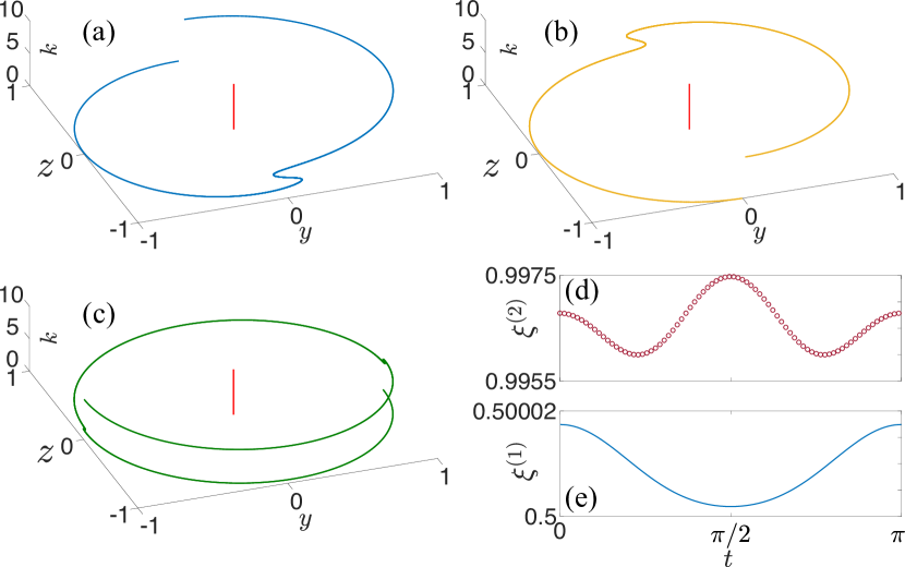
Figure 7: (a) The trajectory of winding vector at time $t=\pi/2$ for the quench protocol in Fig. 4(a) with $\alpha_{f}=0.1$. (b) is similar to (a) but with the protocol in Fig. 4(b) with $\alpha_{f}=0.1$. (c) is similar to (a) but with the protocol in Fig. 4(f) with $\alpha_{f}=6$. (d) and (e) show the time evolution of the $\xi^{(2)}$ and $\xi^{(1)}$ with the quench protocol $\mu=0.5\rightarrow 3$ and other parameters are similar to the quench protocol in Fig. 2(a).

Conventionally, the initial state is chosen as a topologically trivial ground state Gong and Ueda (2018); Chang (2018); Lu and Yu (2019). To investigate if the above statements still hold in the long-range sector, we choose our $H^{i}$ to be in the topologically nontrivial phase with massive Dirac edge states and winding number $w=1/2$, while our $H^{f}$ is a trivial one with $w=-1/2$. Specifically, we quench the chemical potential $\mu=-2\rightarrow-1$ and $2$ separately with $\alpha=0.5$. It is quite remarkable that the TPT can still be characterized by the dynamics of entanglement spectra in this case, as shown in Fig. 2(e). Actually, the half-way winding number of the quench in Fig. 2(e) is $3/2$ (see Fig. 2(f)), different from that of the initial Hamiltonian ($w=1/2$). On the contrary, in the short-range sector, the half-way winding number would still be 1 (for instance, the quench protocol in Fig. 7(d), see Appendix C), same as that of the original Hamiltonian. Consequently, one can see that the characterization of TPTs via entanglement-spectrum dynamics tightly depends on the difference between the winding number of initial Hamiltonian and the half-way winding number. Moreover, similar to Fig. 2(c) and (d), the non-degenerate entanglement-spectrum property can also be explained by the winding number $w=3/2$ (see Appendix D).

It is worthwhile to emphasize that the dynamical behaviors of entanglement spectra close to their crossings are linear in the short-range sector (see Fig 2(a)), just like those in the models with nearest-neighbor interactions Gong and Ueda (2018); Chang (2018); Lu and Yu (2019). In stark contrast, as shown in Fig 2(c) and (e), the behaviors become non-linear in the long-range sector. We present an explanation of this drastic change in Appendix E.

In addition, we study the above quench protocols with a more detailed method. We fix the initial state as a ground state in the phases with $w=1$, $w=-1/2$ and $w=1/2$, i.e., $(\alpha_{i},\mu_{i})=(2,3)$, $(0.5,3)$ and $(0.5,-3)$ respectively, and explore the dependence of the $\xi^{(1)}$ at $t=\pi/2$ (denoted as $\xi^{(1)}(t=\pi/2)$) and $\mu_{f}$. In Fig. 3(a) and (b), with the initial Hamiltonian in the trivial topological phase, $\xi^{(1)}(t=\pi/2)$ shows non-analytical behaviors at the critical points. In Fig. 3(c), one can see that $\xi^{(1)}(t=\pi/2)$ seems to gradually approach 0.5 as $\mu_{f}$ gets closer to the critical point $\mu_{c}=1$. However, at the critical point $\mu_{c}=1$, there is a distinctive behavior of $\xi^{(1)}$. In Appendix D, we show that the singularity of the $\xi^{(1)}$ at the critical point is an artifact of band flatting. With the band flatting, the winding number at $t=\pi/2$ is well-defined as the half-way winding number. When $\mu_{f}>\mu_{c}$, the half-way winding number is $w=3/2$. In contrast, if the quench protocol does not cross $\mu_{c}$, the behavior of $\xi^{(1)}$ is similar to the ground-state entanglement spectra in the topological phase of initial Hamiltonian. More specifically, as shown in Fig. 2(b), the $\xi^{(1)}$ of ground states also gradually approaches 0.5 with $\mu\rightarrow 1$ when $\alpha=0.5$, $\mu<1$, and the winding number $w=1/2$. Thus, it can be predicted that the behavior of the $\xi^{(1)}$ of ground states for the TPT between the topological phase with $w=1/2$ and $w=3/2$ may be similar to that in Fig. 3(c). Indeed, we observe a similar singularity of the ground-state $\xi^{(1)}$ near the critical point of a TPT between the $w=1/2$ and $w=3/2$ phase, indicating that the occurrence of the singularity of the ground-state $\xi^{(1)}$ is closely related to the gapless energy spectra (see Appendix C).

III.2 Decay rate $\alpha$ as the quench parameter

To further explore the dynamics of entanglement spectra in the long-range system, we now turn to consider the quench protocols with the decay rate $\alpha$ as the quench parameter, i.e., $\alpha=\alpha_{i}\rightarrow\alpha_{f}$, while other parameters are fixed. The $\alpha_{i}$ and $\alpha_{f}$ refer to the decay rate of the initial and final Hamiltonian respectively.

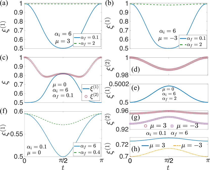
Figure 4: (a) Time evolution of the $\xi^{(1)}$ with the quench protocol $\alpha=6\rightarrow 2$ and $0.1$ in the Hamiltonian (1) with $\mu=3$ and $\Delta=t=1$. (b) is similar to (a) but in the Hamiltonian (1) with $\mu=-3$. (c) Time evolution of the $\xi^{(1)}$ and $\xi^{(2)}$ with the quench protocol $\alpha=6\rightarrow 0.1$ in the Hamiltonian (1) with $\mu=0$ and $\Delta=t=1$. (d) and (e) are similar to (c) but with the the quench protocol $\alpha=6\rightarrow 2$. (f) Time evolution of the $\xi^{(1)}$ with the quench protocol $\alpha=0.1\rightarrow 6$ and $0.4$ in the Hamiltonian (1) with $\mu=0$ and $\Delta=t=1$. (g) and (h) are similar to (f) but in the Hamiltonian (1) with $\mu=\pm 3$.

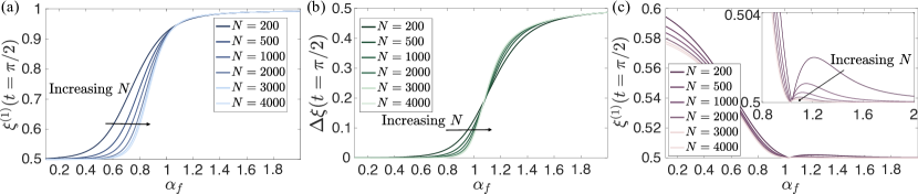
Figure 5: (a) The $\xi^{(1)}(t=\pi/2)$, with the quench protocol $\alpha=6\rightarrow\alpha_{f}$ as a function of $\alpha_{f}$ in the Hamiltonian (1) with $\mu=3$ and different system sizes $N$. (b) The $\Delta\xi(t=\pi/2)$, with the quench protocol $\alpha=6\rightarrow\alpha_{f}$ as a function of $\alpha_{f}$ in the Hamiltonian (1) with $\mu=0$ and different system sizes $N$. Here, the critical points are $\alpha_{c}=1$. (c) is similar to (a) but with the quench protocol $\alpha=0.1\rightarrow\alpha_{f}$ as a function of $\alpha_{f}$ in the Hamiltonian (1) with $\mu=0$. Here, the critical line is $\alpha_{c}=1$.

Fig. 4 (a)-(e) show the quench dynamics of entanglement spectra with the protocol $\alpha=6\rightarrow 0.1$ and $2$. For $\mu=3$ ($-3$), the half-way winding number is $+1$ ($-1$) (see Appendix B for the trajectory of $\bm{d}(\pi/2)$) and the entanglement spectra are non-degenerate at $t=\pi/2$. Thus, we only focus on the $\xi^{(1)}$, whose dynamical behaviors are shown in Fig. 4(a) and (b). The half-way entanglement-spectrum crossings, i.e., $\xi^{(1)}(t=\pi/2)=0.5$ can still characterize the TPTs with the critical line $\alpha_{c}=1$. Next, we study the quench protocol $\alpha=6\rightarrow 0.1$ with $\mu=0$. Different from the previous protocols where the ground-state $\xi^{(1)}$ of $H^{i}$ is larger than that of $H^{f}$, such as the quench protocols in Fig. 4(a) and (b), the ground-state $\xi^{(1)}$ of $H^{i}$ in the current protocol is smaller than that of $H^{f}$. In fact, the $\xi^{(1)}$ of $H^{i}$ is equal to $0.5$, as depicted in Fig. 1(b). Remarkably, as shown in Fig. 4(c), (d) and (e), instead of the entanglement-spectrum crossings $\xi=1/2$, the TPTs can be alternatively characterized by a novel behavior of the entanglement spectra, i.e., $\xi^{(1)}(t=\pi/2)=\xi^{(2)}(t=\pi/2)$ when quenching across the critical line $\alpha_{c}=1$ ($\alpha_{f}=0.1$), while there is a large discrepancy between $\xi^{(1)}(t=\pi/2)$ and $\xi^{(2)}(t=\pi/2)$ when staying the same phase ($\alpha_{f}=2$).

In addition, we also study the inverse of above protocols. Fig. 4 (f)-(h) show the quench dynamics of entanglement spectra with the protocol $\alpha=0.1\rightarrow 6$ and $0.4$. For $\mu=0$, the ground-state $\xi^{(1)}$ of $H^{i}$ is larger than that of $H^{f}$, and the dynamical entanglement-spectrum properties are similar to Fig. 4(a) and (b). For $\mu=\pm 3$, even if the quenches cross the critical line $\alpha_{c}=1$, $\xi^{(1)}(t=\pi/2)=\xi^{(2)}(t=\pi/2)$ is not satisfied, and the ES dynamics fails to characterize the TPTs. Actually, in comparison with the quench protocol in Fig. 4 (c) where the half-way winding number ($w=0$) is different from that of initial Hamiltonian ($w=1$), for the quench protocol in Fig. 4 (g) and (h), the dynamics of entanglement spectra is predicted to be trivial since the winding number of initial Hamiltonian is equal to the half-way winding number. Complementary with previous results in Fig. 2 and Fig. 7(d), one can see that the difference between half-way winding number and the winding number of initial Hamiltonian is tightly related to the capability of entanglement-spectrum dynamics in identifying TPTs.

We then fix the initial Hamiltonian with the parameters $(\alpha_{i},\mu_{i})=(6,3)$, $(6,0)$ and $(0.1,0)$, and explore the entanglement spectra at $t=\pi/2$ as a function of $\alpha_{f}$. In Fig. 5(a), the dependence of the $\xi^{(1)}(t=\pi/2)$ and $\alpha_{f}$ with the quench protocols $\alpha=6\rightarrow\alpha_{f}$ and $\mu=3$ is presented. One can see that the results of system size $N=200$ suffers from finite-size effect. Thus, we further calculate the results of larger system size $N=500-4000$. When increasing $N$, the change of $\xi^{(1)}(t=\pi/2)$ becomes more dramatic at the critical point $\alpha_{c}=1$. To study another quench protocols $\alpha=6\rightarrow\alpha_{f}$ with $\mu=0$, we focus on the difference between the first and second lowest entanglement-spectrum value at $t=\pi/2$, i.e., $\Delta\xi=\xi^{(2)}-\xi^{(1)}$. The difference of the entanglement spectra $\Delta\xi(t=\pi/2)$ as a function of $\alpha_{f}$ is shown in Fig. 5(b). Similar to the results in Fig. 5(a), with the increase of $N$, the entanglement-spectrum critical behavior becomes more obvious. In Fig. 5(c), we present the results of the quench protocols $\alpha=0.1\rightarrow\alpha_{f}$ with $\mu=0$, as the quenches with opposite direction of these in Fig. 5(b). On this condition, the finite-size effect is smaller, and it can be directly inferred that the $\xi^{(1)}(t=\pi/2)$ has finite value for $\alpha_{f}<\alpha_{c}$ while vanishes for $\alpha_{f}>\alpha_{c}$ ($\alpha_{c}=1$) when $N\rightarrow\infty$.

It is noted that the finite-size effects in long-range systems may be peculiar, and the crossing point of all the curves may not necessarily correspond to the critical point (an example is given in Ref. Emary and Brandes (2003)). In Fig. 5(a) and (b), the results of $\xi^{(1)}(t=\pi/2)$ show a strong finite-size effect. To better understand the finite-size effect in long-range sector, in Fig. 6), we plot the half-way winding number $w(t=\pi/2)$ as a function of $\alpha_{f}$ with the same quench protocol in Fig. 5(a) and (b), showing that the finite-size behaviors of $w(t=\pi/2)$ are similar to these of $\xi^{(1)}(t=\pi/2)$.

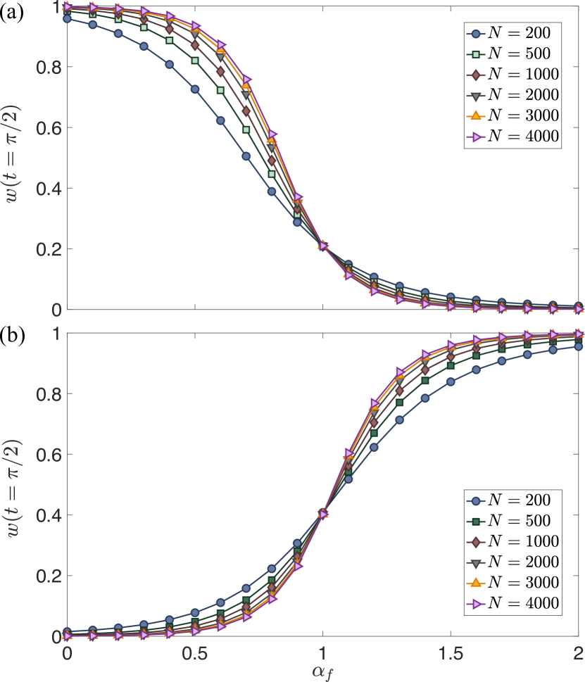
Figure 6: (a) The half-way winding number $w(t=\pi/2)$ as a function of $\alpha_{f}$ with the quench protocol in Fig. 5(a). (b) is similar to (a) but with the quench protocol in Fig. 5(b).

IV Summary and outlook

Recent works Gong and Ueda (2018); Chang (2018); Lu and Yu (2019) show that the TPTs in the systems with nearest-neighbor interactions can be characterized by the quench dynamics of entanglement spectra. By studying the out-of-equilibrium properties of entanglement spectra in the long-range Kitaev chain with power-law decay pairing terms, we have found that: (i) in the short-range sector (decay rate $\alpha>1$), the entanglement-spectrum behaviors are similar to these in the conventional Kitaev chain Lu and Yu (2019), i.e., when quenching across the critical line and the initial Hamiltonian is topologically trivial, the entanglement-spectrum crossings $\xi=1/2$ are observed. (ii) In the long-range sector (decay rate $\alpha<1$), for both topologically trivial or non-trivial initial Hamiltonian, the entanglement-spectrum crossings can still characterize the TPTs via entanglement-spectrum crossing. However, the entanglement-spectrum crossings vanish for the topologically trivial final Hamiltonian in the short-range sector even if the quench protocols cross the critical lines. (iii) For the quench protocols with decay rate $\alpha$ as the quench parameter, the entanglement-spectrum dynamics can diagnose TPTs when the winding number of initial Hamiltonian is different from the half-way winding number. Besides the entanglement-spectrum crossings, one can also characterize the TPTs by studying the difference between the first and second lowest entanglement-spectrum value in the special case. In a word, the characterization of TPTs via the quench dynamics of entanglement spectra could be well generalized to long-range systems. Moreover, we emphasize that although the following results are based on the band-flattened Hamiltonian, as shown in Appendix D, the TPTs can still be characterized by the entanglement-spectrum crossings for the post-quench Hamiltonian without flat bands.

This work may inspire further investigations on the quench dynamics of entanglement spectra in several long-range systems, for instance, the characterization of the topological phases with higher winding number in the longer-range Kitaev chains Zhang and Song (2015); Alecce and Dell’Anna (2017), the TPTs in the two-dimensional topological superconductors with long-range interactions Viyuela et al. (2018), the conventional quantum phase transitions Koffel et al. (2012) or dynamical phase transitions Žunkovič et al. (2018); Xu et al. (2019); Sedlmayr et al. (2018); Masłowski and Sedlmayr (2019) in long-range systems.

Appendix A The antiperiodic boundary condition

For the long-range Kitaev chain with power-law decay pairing terms, we adopt the antiperiodic boundary condition $c_{i+N}=-c_{i}$. Here, we discuss the reason behind the choice of the antiperiodic boundary condition in detail.

In the Hamiltonian (1), the term describing the power-law decay pairing interactions can be regrouped, i.e., $\sum_{i=1}^{N}\sum_{l=1}^{N-i}\frac{1}{d_{l}^{\alpha}}(c_{i}c_{i+l}+\text{H.c.})=\sum_{i=1}^{N}\sum_{i=1}^{N-l}\frac{1}{d_{l}^{\alpha}}(c_{i}c_{i+l}+\text{H.c.})$. Then, we can pick the $l$ nearest terms $\sum_{i=1}^{N-l}\frac{1}{d_{l}^{\alpha}}(c_{i}c_{i+l}+\text{H.c.})$ and $N-l$ nearest $\sum_{i=1}^{l}\frac{1}{d_{N-l}^{\alpha}}(c_{i}c_{i+N-l}+\text{H.c.})$. We note that the coefficients of the $l$ and $N-l$ nearest terms are actually the same since $d_{l}=d_{N-l}$. As a consequence, taking $l=1$ for example, we can see $c_{1}c_{2}+\ldots+c_{N-1}c_{N}+(c_{1}c_{N})=c_{1}c_{2}+\ldots+c_{N-1}c_{N}-c_{1}c_{N}$. Next, imposing the antiperiodic boundary condition $c_{i+N}=-c_{i}$, we have $c_{1}c_{2}+\ldots+c_{N-1}c_{N}+c_{N}c_{N+1}$, which allows us to switch the Hamiltonian to the Fourier basis. If the periodic boundary condition is imposed, the coefficients of the $l$ and $N-l$ nearest terms should be the opposite of each other.

Appendix B The details of calculating the quench dynamics of entanglement spectra

After obtaining the winding vector at arbitary time $t$ during the quench dynamics according to Eq. (6), we can diagonalize the Hamiltonian at $t$, i.e., $H(t)=\sum_{k}\epsilon_{k}\Psi_{k}^{\dagger}(\bm{d}_{k}(t)\cdot\bm{\sigma})\Psi_{k}$ , via the Bogoliubov transformation

$$\Psi_{k}^{\dagger}(\bm{d}_{k}(t)\cdot\bm{\sigma})\Psi_{k}=\Psi_{k}^{\dagger}V_{k}(t)\Lambda_{k}(t)V_{k}^{\dagger}(t)\Psi_{k},$$ (10)

giving the Bogoliubov fermion operators at $t$, i.e., $(a_{-k}(t),a_{k}^{\dagger}(t))=\Psi_{k}^{\dagger}V_{k}(t)$, which satisfies $a_{k}(t)|\text{Vac}\rangle$ =0. The two-dimension unitary matrix $V_{k}$, whose elements are denoted as $v_{ij}(k)$ $(i,j\in\{1,2\})$, is the key to calculate the correlation matrix

$$C_{mn} = \langle\text{Vac}|c_{m}^{\dagger}c_{n}|\text{Vac}\rangle$$ (11)

$$= \frac{1}{N}\sum_{k}e^{-ik(m-n)}v_{22}(k)v^{*}_{22}(k)$$

$$+ e^{ik(m-n)}v_{11}(k)v^{*}_{11}(k),$$

and anomalous correlation matrix,

$$F_{mn} = \langle\text{Vac}|c_{m}^{\dagger}c_{n}^{\dagger}|\text{Vac}\rangle$$ (12)

$$= \frac{1}{N}\sum_{k}e^{-ik(m-n)}v_{22}(k)v^{*}_{12}(k)$$

$$+ e^{ik(m-n)}v_{21}(k)v^{*}_{11}(k),$$

which are useful for obtaining the entanglement spectra.

The value of $\Omega_{q}$ in Eq. (8) can be obtained by the diagonalization of a matrix composed of the correlation matrix and anomalous correlation matrix, i.e.,

$$\begin{pmatrix}I-C_{\mathcal{A}}^{*}&-F_{\mathcal{A}}^{*}\\ F_{\mathcal{A}}&C_{\mathcal{A}}\end{pmatrix}=P^{\dagger}\begin{pmatrix}\Xi^{-}&0\\ 0&\Xi^{+}\end{pmatrix}P,$$ (13)

with $\Xi^{\pm}$ as diagonal matrix whose elements are $1/(1+e^{\pm\Omega_{q}})$.

Appendix C Additional results

In this appendix, we present some addition results, including the trajectory of winding vector at time $t=\pi/2$ and time evolution of the entanglement spectra for some quench protocols.

Appendix D Extended Kitaev chains with long-range pairing and the topological phase with $w=3/2$

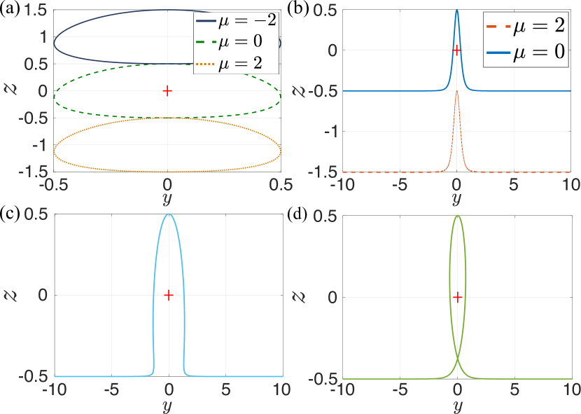
Figure 8: The trajectory of winding vector in the Hamiltonian (14) with (a) $\alpha=2$, $\Delta=t=1$, $\delta=0$, and $\mu=-2$, $0$, $2$. The winding number $w=1$ for $\mu=0$ and $w=0$ for $\mu=\pm 2$. (b) $\alpha=0.5$, $\Delta=t=1$, $\delta=0$, and $\mu=0$, $2$. The winding number $w=1/2$ for $\mu=0$ and $w=-1/2$ for $\mu=2$. (c) $\mu=0$, $\alpha=0.5$, $t=\Delta=1$, and $\delta=2$. The winding number $w=1/2$. (d) $\mu=0$, $\alpha=0.5$, $t=\Delta=1$, and $\delta=-2$. The winding number $w=3/2$.

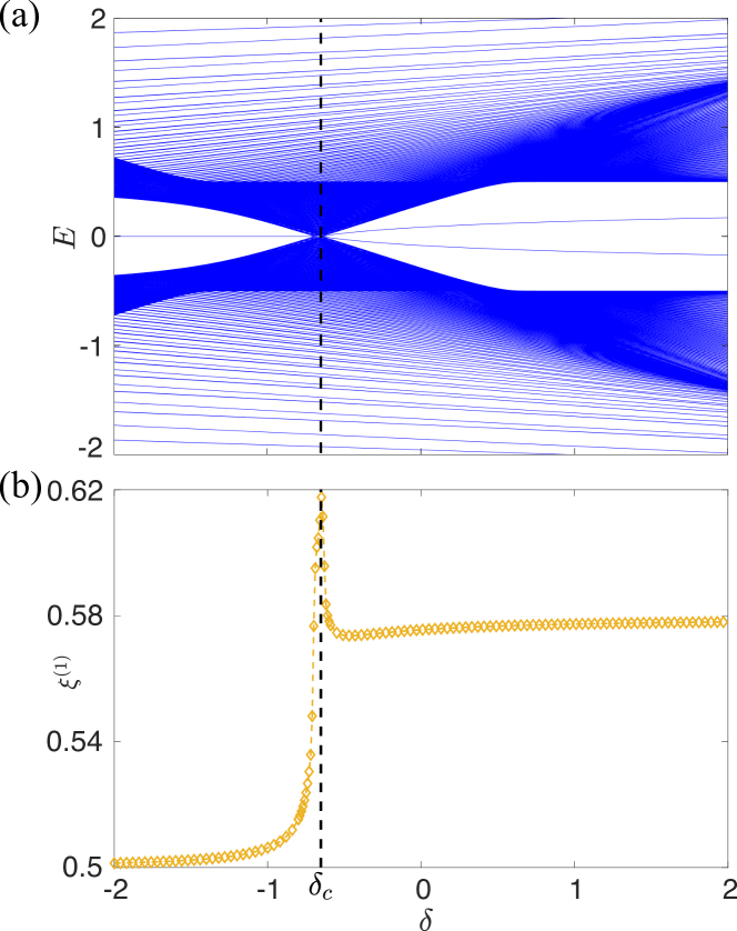
Figure 9: (a) The energy spectrum for the Hamiltonian (14) as a function of $\delta$. (b) The $\xi^{(1)}$ as a function of $\delta$ for the ground state of the Hamiltonian (14). Here, the other parameters are $\mu=0$, $\alpha=0.5$, and $t=\Delta=1$.

Here, we consider a new Hamiltonian with the open boundary condition

$$H= - \frac{t}{2}\sum_{i=1}^{N}(c_{i}^{\dagger}c_{i+1}+\text{H.c.})-\mu\sum_{i=1}^{N}(c_{i}^{\dagger}c_{i}-\frac{1}{2})$$ (14)

$$+ \frac{\Delta}{2}\sum_{i=1}^{N-l}\sum_{l=1}^{N/2-1}\frac{1}{d_{l}^{\alpha}}(c_{i}c_{i+l}+\text{H.c.})$$

$$+ \frac{\delta}{2}\sum_{i=1}^{N-1}(c_{i}c_{i+1}+\text{H.c.}).$$

It is noted that the summation notation of the long-range pairing term $\frac{1}{d_{l}^{\alpha}}(c_{i}c_{i+l}+\text{H.c.})$ is sightly different from the one in Eq. (1) because of the cutoff of the power-law decay $N/2-1$ for convenience. The winding vector of the Hamiltonian (14) reads

$$\bm{d}_{k} = (d_{k}^{x},d_{k}^{y},d_{k}^{z})$$ (15)

$$= (0,-\frac{(\Delta f_{\alpha}(k)+\delta\sin k)}{2},-\frac{(\mu+t\cos k)}{2}).$$

Then, we plot the the trajectory of the winding vector, obtaining the related winding number. In Fig. 8(a) and (b), we show that with $\delta=0$, the winding numbers of the topological phases in Hamiltonian (14) are the same as these in Hamiltonian (1). Thus, the cutoff of the power-law decay $N/2-1$ does not influence the phase diagram of the Hamiltonian. More importantly, with $\mu=0$, $\alpha=0.5$, and $t=\Delta=1$, as shown in Fig. 8(c) and (d), the winding number is equal to $1/2$ and $3/2$ for $\delta=2$ and $-2$ respectively. Actually, by tuning $\delta$ from $2$ to $-2$, there is a TPT between the topological phases with $w=1/2$ and $w=3/2$.

In addition, we also present the energy spectrum as a function of $\delta=2$ with $\mu=0$, $\alpha=0.5$, and $t=\Delta=1$ in Fig. 9(a). One can see that there are massive Dirac edge states in the topological phase with $w=1/2$ (for instance, $\delta=2$), and one pair of Majorana zero modes is present in the topological phase with $w=3/2$ (for instance, $\delta=-2$). We also calculate the $\xi^{(1)}$ for the ground state, which is plotted in Fig. 9(b). For $\delta<\delta_{c}$, $\xi^{(1)}\simeq 0.5$, corresponding to the one pair of Majorana zero modes, while $\xi^{(1)}$ has a larger value when $\delta>\delta_{c}$ and massive Dirac edge states are observed. There is a singularity of $\xi^{(1)}$ close to the critical point $\delta_{c}$, which is connected with the gapless energy spectrum. In contrast, as shown in Fig. 1(b), the singularity of $\xi^{(1)}$ is absent at the critical line $\alpha_{c}=1$ since the energy spectrum is gapped (see Fig. 1(c) and (d)).

It is noted that with the same parameters of the topological phase $w=3/2$ in the Hamiltonian (14), after performing a gauge transformation $c_{j}\rightarrow c_{j}e^{i\frac{\pi}{2}}$, the winding number becomes $w=-3/2$. Since the gauge transformation does not influence the topological properties of the system, it is predicted that there is also one pair of Majorana zero modes in the topological phase with $w=-3/2$, which corresponds to the entanglement-spectrum non-degeneracy in Fig. 2(e).

Appendix E An explanation of the non-linear behaviors of $\xi^{(1)}$ near $t=\pi/2$

In this Appendix, we present a perturbation study to explain the linear and non-linear behaviors of $\xi^{(1)}$ around $t=\pi/2$ in the short-range and long-range sector respectively. According to Eq. (9), $\xi_{q}\propto\lambda_{q}$, and thus we can perform a perturbation study of the eigenenergies to understand the entanglement-spectrum properties.

From Eq.(6), only keeping the linear term, we have

$$\Delta\bm{d}_{k} = \bm{d}_{k}(\pi/2+\Delta t)-\bm{d}_{k}(\pi/2)$$ (16)

$$= -2\Delta t[\bm{d}_{k}^{i}\times\bm{n}_{k}^{f}].$$

Thus, the perturbation problem now reduces to perturbing the half-way Hamiltonian $H_{0}$ with $-2\Delta tV$ with $V$ as the Hamiltonian corresponding to $\bm{d}_{k}^{i}\times\bm{n}_{k}^{f}$. It is seen that the perturbation term preserves the particle-hole symmetry, but breaks the time reversal symmetry, i.e., $\mathcal{P}V\mathcal{P}^{-1}=-V$ and $\mathcal{T}V\mathcal{T}^{-1}=-V$.

We now focus on the lowest two eigenstates of the half-way Hamiltonian, and denote the eigenmodes as $c_{1}$ and $c_{2}$. The couplings between $V$ and the two eigenmodes can be described by a four-level effective model $V=\psi^{\dagger}V_{\text{eff}}\psi$, where $\psi^{\dagger}=(c_{1}^{\dagger},c_{2}^{\dagger},c_{1},c_{2})$, and

$$V_{\text{eff}}=\begin{pmatrix}A&B\\ -B^{*}&-A^{*}\\ \end{pmatrix}$$ (17)

with $A$ and $B$ as 2-dimensional matrix. The above structure is a requirement of particle-hole symmetry. Then, considering $\mathcal{T}V\mathcal{T}^{-1}=-V$, We recognize that $A=-A^{*}$ and $B=-B^{*}$. Moreover, because of the anti-communication relation, the matrix $A$ is eliminated and $B$ should be anti-symmetric. Finally, the form of $V_{\text{eff}}$ can be fixed as

$$V_{\text{eff}}\propto\begin{pmatrix}0&0&0&i\\ 0&0&-i&0\\ 0&i&0&0\\ -i&0&0&0\end{pmatrix},$$

i.e., $V_{\text{eff}}\propto i(c_{2}c_{1}-c_{1}^{\dagger}c_{2}^{\dagger})$.

In the short-range sector, the zero energy modes are degenerate, and can be decomposed into Majorana operators residing on the left and right end of the chain. Specifically, we have $c_{i}=a_{i}+ib_{i}$ ($i=1,2$), and $V_{\text{eff}}\propto-2i(a_{1}a_{2}+b_{2}b_{1})$. It directly couples Majorana modes on the same side, giving a linear contribution to the energy.

In the long-range sector, $c_{1}$ is still massless, while $c_{2}$ becomes massive. Here,

$$H_{0}-2\Delta tV_{\text{eff}}\propto\begin{pmatrix}0&0&0&i\Delta t^{\prime}\\ 0&\epsilon&-i\Delta t^{\prime}&0\\ 0&i\Delta t^{\prime}&0&0\\ -i\Delta t^{\prime}&0&0&-\epsilon\end{pmatrix}$$

with $\epsilon\neq 0$ since $c_{2}$ denotes a massive mode, and $\Delta t^{\prime}$ as a normalized perturbation parameter proportional to $\Delta t$. The eigenvalues of the matrix are

$$\lambda^{(1)}_{\pm}=\sqrt{(\frac{\epsilon}{2})^{2}+(\Delta t^{\prime})^{2}}\pm\frac{\epsilon}{2}$$ (18)

$$\lambda^{(2)}_{\pm}=-\sqrt{(\frac{\epsilon}{2})^{2}+(\Delta t^{\prime})^{2}}\pm\frac{\epsilon}{2}.$$

We note that $V$ also contains other terms that couple $c_{1}$ and $c_{2}$ to other bulk modes. Nevertheless, these terms do not give any contributions in the leading order, and thus do not influence the above analysis. Since we have shown that in the long-range sector, the eigenvalues can be regarded as non-linear functions of $\Delta t$, the above discussion explains the difference between the behaviors of $\xi^{(1)}$ near $t=\pi/2$ in the short-range and long-range sector.

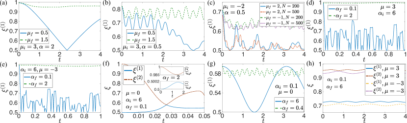
Figure 10: The quench dynamics of entanglement spectra for the post-quench Hamiltonian without flat bands. The quanch protocol in (a)-(e) is the same as that in Fig. 2(a), Fig. 2(c), Fig. 2(e), Fig. 4(a) and Fig. 4(b), respectively. The quench protocol in (f) is the same as that in Fig. 4(c)-(e). The quench protocol in (g) is the same as that in Fig. 4(f). The quench protocol in (h) is the same as that in Fig. 4(g) and (h).

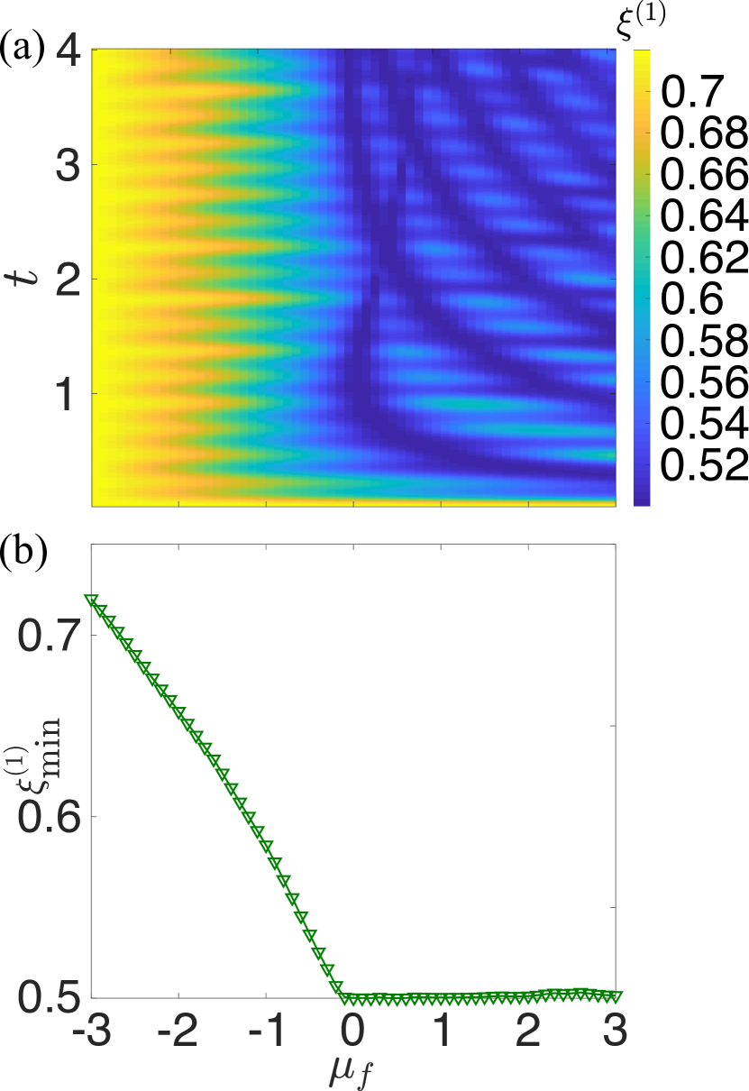
Figure 11: (a) The $\xi^{(1)}$ plotted in the $t$-$\mu_{f}$ plane. (b) The $\xi^{(1)}_{\text{min}}$ as a function of $\mu_{f}$.

Appendix F Results of the post-quench Hamiltonian without flat bands

In this Appendix, we present the quench dynamics of entanglement spectra with the same quench protocols in Fig. 2(a), (c), (e) and Fig. 4. The results are shown in Fig 10, indicating that the conclusions made in the flat-band case are stable. Indeed, it has been shown that the occurrence of entanglement-spectrum crossings is stable for the conventional Kitaev chain with nearest interactions in class D Lu and Yu (2019). Here, we demonstrate that the stability of the crossings can be generalized to the long-range Kitaev chain.

It is noted that a distinctive fast oscillating entanglement-spectrum behavior can be observed when the initial or finial Hamiltonian is in the long-range sector. For instance, the oscillation of entanglement spectra is more dramatic in Fig. 10(b) than that in Fig. 10(a). The oscillating behavior may be related to the divergence of quasiparticle energy since for the Hamiltonian (1), the divergence of $\epsilon_{k}$ can occur when $k=0$ or $2\pi$ in the long-range sector $\alpha<1$ Van Regemortel et al. (2016).

Furthermore, we study the quench dynamics of $\xi^{(1)}$ without flat bands in detail. The initial state is chosen as a ground state of Hamiltonian (1) with $(\alpha_{i},\mu_{i})=(0.5,-3)$, and $\mu_{f}$ varies from -3 to 3. In Fig. 11(a), it is shown that although $\mu_{f}<\mu_{c}$ ($\mu_{c}=1$), the $\xi^{(1)}$ approaches 0.5 during its time evolution. Moreover, we can employ the minimum entanglement-spectrum value $\xi^{(1)}_{\text{min}}=\min_{t\in[0,t_{f}]}\xi^{(1)}(t)$ with ($t_{f}=4$) to clarify whether the quench dynamics of entanglement spectra can efficiently detect the TPT without flat bands. The $\xi^{(1)}_{\text{min}}$ as a function of $\mu_{f}$ is plotted in Fig. 11(b). It is noted that the quench protocol in Fig. 11 is the same as that in Fig. 3(c). However, the entanglement-spectrum singular behavior near the critical point vanishes without flat bands.

Here, we emphasize that although the qualitative behaviors of the entanglement spectra are stable against energy dispersion (see Fig. 10), in Fig. 11(b), the $\xi^{(1)}_{\text{min}}$ is trivial around the critical point $\mu_{c}=1$. As a consequence, the characterization of TPTs via the entanglement-spectrum dynamics in the long-range system without flat bands remains an open and complex problem, and deserves a more special study.

References

- Qi and Zhang (2011) X.-L. Qi and S.-C. Zhang, Rev. Mod. Phys. 83, 1057 (2011).
- Sato and Ando (2017) M. Sato and Y. Ando, Reports on Progress in Physics 80, 076501 (2017).
- Nadj-Perge et al. (2014) S. Nadj-Perge, I. K. Drozdov, J. Li, H. Chen, S. Jeon, J. Seo, A. H. MacDonald, B. A. Bernevig, and A. Yazdani, Science 346, 602 (2014).
- Mourik et al. (2012) V. Mourik, K. Zuo, S. M. Frolov, S. R. Plissard, E. P. A. M. Bakkers, and L. P. Kouwenhoven, Science 336, 1003 (2012).
- Sarma et al. (2015) S. D. Sarma, M. Freedman, and C. Nayak, Npj Quantum Information 1, 15001 (2015).
- Mong et al. (2014) R. S. K. Mong, D. J. Clarke, J. Alicea, N. H. Lindner, P. Fendley, C. Nayak, Y. Oreg, A. Stern, E. Berg, K. Shtengel, and M. P. A. Fisher, Phys. Rev. X 4, 011036 (2014).
- Kraus et al. (2013) C. V. Kraus, P. Zoller, and M. A. Baranov, Phys. Rev. Lett. 111, 203001 (2013).
- Alicea (2012) J. Alicea, Reports on Progress in Physics 75, 076501 (2012).
- Kitaev (2003) A. Kitaev, Annals of Physics 303, 2 (2003).
- Viyuela et al. (2016) O. Viyuela, D. Vodola, G. Pupillo, and M. A. Martin-Delgado, Phys. Rev. B 94, 125121 (2016).
- Choi et al. (2017) D.-J. Choi, C. Rubio-Verdú, J. de Bruijckere, M. M. Ugeda, N. Lorente, and J. I. Pascual, Nature Communications 8, 15175 (2017).
- Ménard et al. (2017) G. C. Ménard, S. Guissart, C. Brun, R. T. Leriche, M. Trif, F. Debontridder, D. Demaille, D. Roditchev, P. Simon, and T. Cren, Nature Communications 8, 2040 (2017).
- Ménard et al. (2015) G. C. Ménard, S. Guissart, C. Brun, S. Pons, V. S. Stolyarov, F. Debontridder, M. V. Leclerc, E. Janod, L. Cario, D. Roditchev, P. Simon, and T. Cren, Nature Physics 11, 1013 (2015).
- Neupert et al. (2016) T. Neupert, A. Yazdani, and B. A. Bernevig, Phys. Rev. B 93, 094508 (2016).
- Pientka et al. (2014) F. Pientka, L. I. Glazman, and F. von Oppen, Phys. Rev. B 89, 180505(R) (2014).
- Klinovaja et al. (2013) J. Klinovaja, P. Stano, A. Yazdani, and D. Loss, Phys. Rev. Lett. 111, 186805 (2013).
- Nadj-Perge et al. (2013) S. Nadj-Perge, I. K. Drozdov, B. A. Bernevig, and A. Yazdani, Phys. Rev. B 88, 020407(R) (2013).
- Pientka et al. (2013) F. Pientka, L. I. Glazman, and F. von Oppen, Phys. Rev. B 88, 155420 (2013).
- Kaladzhyan et al. (2016) V. Kaladzhyan, C. Bena, and P. Simon, Journal of Physics: Condensed Matter 28, 485701 (2016).
- Heinrich et al. (2018) B. W. Heinrich, J. I. Pascual, and K. J. Franke, Progress in Surface Science 93, 1 (2018).
- Li and Sun (2018) S.-P. Li and Z.-H. Sun, Phys. Rev. A 98, 022317 (2018).
- Qiao et al. (2019) H. Qiao, Z.-H. Sun, F.-X. Sun, L.-Z. Mu, Q. He, and H. Fan, Annals of Physics 411, 167967 (2019).
- Pezzè et al. (2017) L. Pezzè, M. Gabbrielli, L. Lepori, and A. Smerzi, Phys. Rev. Lett. 119, 250401 (2017).
- Zhang et al. (2018a) Y.-R. Zhang, Y. Zeng, H. Fan, J. Q. You, and F. Nori, Phys. Rev. Lett. 120, 250501 (2018a).
- Gabbrielli et al. (2018) M. Gabbrielli, A. Smerzi, and L. Pezzè, Scientific Reports 8, 15663 (2018).
- Yin et al. (2019) S. Yin, J. Song, Y. Zhang, and S. Liu, Phys. Rev. B 100, 184417 (2019).
- Kitaev and Preskill (2006) A. Kitaev and J. Preskill, Phys. Rev. Lett. 96, 110404 (2006).
- Levin and Wen (2006) M. Levin and X.-G. Wen, Phys. Rev. Lett. 96, 110405 (2006).
- Vodola et al. (2014) D. Vodola, L. Lepori, E. Ercolessi, A. V. Gorshkov, and G. Pupillo, Phys. Rev. Lett. 113, 156402 (2014).
- Fromholz et al. (2019) P. Fromholz, G. Magnifico, V. Vitale, T. Mendes-Santos, and M. Dalmonte, ArXiv e-prints (2019), arXiv:1909.04035 [quant-ph] .
- Li and Haldane (2008) H. Li and F. D. M. Haldane, Phys. Rev. Lett. 101, 010504 (2008).
- Pollmann et al. (2010) F. Pollmann, A. M. Turner, E. Berg, and M. Oshikawa, Phys. Rev. B 81, 064439 (2010).
- Fidkowski (2010) L. Fidkowski, Phys. Rev. Lett. 104, 130502 (2010).
- Gross and Bloch (2017) C. Gross and I. Bloch, Science 357, 995 (2017).
- Fläschner et al. (2018) N. Fläschner, D. Vogel, M. Tarnowski, B. S. Rem, D.-S. Lühmann, M. Heyl, J. C. Budich, L. Mathey, K. Sengstock, and C. Weitenberg, Nature Physics 14, 265 (2018).
- Sun et al. (2018) W. Sun, C.-R. Yi, B.-Z. Wang, W.-W. Zhang, B. C. Sanders, X.-T. Xu, Z.-Y. Wang, J. Schmiedmayer, Y. Deng, X.-J. Liu, S. Chen, and J.-W. Pan, Phys. Rev. Lett. 121, 250403 (2018).
- Blatt and Roos (2012) R. Blatt and C. F. Roos, Nature Physics 8, 277 (2012).
- Neill et al. (2017) C. Neill, P. Roushan, M. Fang, Y. Chen, M. Kolodrubetz, Z. Chen, A. Megrant, R. Barends, B. Campbell, B. Chiaro, A. Dunsworth, E. Jeffrey, J. Kelly, J. Mutus, P. J. J. O’Malley, C. Quintana, D. Sank, A. Vainsencher, J. Wenner, T. C. White, A. Polkovnikov, and J. M. Martinis, Nature Physics 12, 1037 (2017).
- Yan et al. (2019) Z. Yan, Y.-R. Zhang, M. Gong, Y. Wu, Y. Zheng, S. Li, C. Wang, F. Liang, J. Lin, Y. Xu, C. Guo, L. Sun, C.-Z. Peng, K. Xia, H. Deng, H. Rong, J. Q. You, F. Nori, H. Fan, X. Zhu, and J.-W. Pan, Science 364, 753 (2019).
- Wilson et al. (2016) J. H. Wilson, J. C. W. Song, and G. Refael, Phys. Rev. Lett. 117, 235302 (2016).
- Wang et al. (2017) C. Wang, P. Zhang, X. Chen, J. Yu, and H. Zhai, Phys. Rev. Lett. 118, 185701 (2017).
- Maffei et al. (2018) M. Maffei, A. Dauphin, F. Cardano, M. Lewenstein, and P. Massignan, New Journal of Physics 20, 013023 (2018).
- Zhang et al. (2018b) L. Zhang, L. Zhang, S. Niu, and X.-J. Liu, Science Bulletin 63, 1385 (2018b).
- Potter et al. (2016) A. C. Potter, T. Morimoto, and A. Vishwanath, Phys. Rev. X 6, 041001 (2016).
- Su et al. (1979) W. P. Su, J. R. Schrieffer, and A. J. Heeger, Phys. Rev. Lett. 42, 1698 (1979).
- Kitaev (2001) A. Y. Kitaev, Physics-Uspekhi 44, 131 (2001).
- Gong and Ueda (2018) Z. Gong and M. Ueda, Phys. Rev. Lett. 121, 250601 (2018).
- Chang (2018) P.-Y. Chang, Phys. Rev. B 97, 224304 (2018).
- Lu and Yu (2019) S. Lu and J. Yu, Phys. Rev. A 99, 033621 (2019).
- Xu et al. (2018) K. Xu, J.-J. Chen, Y. Zeng, Y.-R. Zhang, C. Song, W. Liu, Q. Guo, P. Zhang, D. Xu, H. Deng, K. Huang, H. Wang, X. Zhu, D. Zheng, and H. Fan, Phys. Rev. Lett. 120, 050507 (2018).
- Lanyon et al. (2018) B. P. Lanyon, C. Maier, M. Holzäpfel, T. Baumgratz, C. Hempel, P. Jurcevic, I. Dhand, A. S. Buyskikh, A. J. Daley, M. Cramer, M. B. Plenio, R. Blatt, and C. F. Roos, Nature Physics 13, 1158 (2018).
- Choo et al. (2018) K. Choo, C. W. von Keyserlingk, N. Regnault, and T. Neupert, Phys. Rev. Lett. 121, 086808 (2018).
- Chiu et al. (2016) C.-K. Chiu, J. C. Y. Teo, A. P. Schnyder, and S. Ryu, Rev. Mod. Phys. 88, 035005 (2016).
- Cheong and Henley (2004) S.-A. Cheong and C. L. Henley, Phys. Rev. B 69, 075111 (2004).
- Hughes et al. (2011) T. L. Hughes, E. Prodan, and B. A. Bernevig, Phys. Rev. B 83, 245132 (2011).
- Kitaev (2009) A. Kitaev, AIP Conf. Proc. 1134, 22 (2009).
- Emary and Brandes (2003) C. Emary and T. Brandes, Phys. Rev. E 67, 066203 (2003).
- Zhang and Song (2015) G. Zhang and Z. Song, Phys. Rev. Lett. 115, 177204 (2015).
- Alecce and Dell’Anna (2017) A. Alecce and L. Dell’Anna, Phys. Rev. B 95, 195160 (2017).
- Viyuela et al. (2018) O. Viyuela, L. Fu, and M. A. Martin-Delgado, Phys. Rev. Lett. 120, 017001 (2018).
- Koffel et al. (2012) T. Koffel, M. Lewenstein, and L. Tagliacozzo, Phys. Rev. Lett. 109, 267203 (2012).
- Žunkovič et al. (2018) B. Žunkovič, M. Heyl, M. Knap, and A. Silva, Phys. Rev. Lett. 120, 130601 (2018).
- Xu et al. (2019) K. Xu, Z.-H. Sun, W. Liu, Y.-R. Zhang, H. Li, H. Dong, W. Ren, P. Zhang, F. Nori, D. Zheng, H. Fan, and H. Wang, ArXiv e-prints (2019), arXiv:1912.05150 [quant-ph] .
- Sedlmayr et al. (2018) N. Sedlmayr, P. Jaeger, M. Maiti, and J. Sirker, Phys. Rev. B 97, 064304 (2018).
- Masłowski and Sedlmayr (2019) T. Masłowski and N. Sedlmayr, ArXiv e-prints (2019), arXiv:1911.02831 [quant-ph] .
- Van Regemortel et al. (2016) M. Van Regemortel, D. Sels, and M. Wouters, Phys. Rev. A 93, 032311 (2016).