Large-$N$ behavior of three-dimensional lattice CP^N-1 models

Abstract

We investigate the phase diagram and critical behavior of a three-dimensional lattice CP^N-1 model in the large-$N$ limit. Numerical evidence of first-order transitions is always observed for sufficiently large values of $N$, i.e. $N>2$ up to $N=100$. The transition becomes stronger—both the latent heat and the surface tension increase—as $N$ increases. Moreover, on the high-temperature side, gauge fields decorrelate on distances of the order of one lattice spacing for all values of $N$ considered. Our results are consistent with a simple scenario, in which the transition is of first order for any $N$, including $N\to\infty$. We critically discuss the analytic large-$N$ calculations that predicted a large-$N$ continuous transition, showing that one crucial assumption made in these computations fails for the model we consider.

1 Introduction

Models that are invariant under a local U(1) gauge symmetry have been systematically studied in condensed-matter and in high-energy physics. The simplest model with a local U(1) gauge symmetry is the CP^N-1 model. In three dimensions it emerges as an effective theory describing several condensed-matter systems [1, 2, 3, 4, 5, 6, 7], while in two dimensions it is an interesting theoretical laboratory to study quantum field theories of fundamental interactions as it shares several features with quantum chromodynamics (QCD), the theory that describes the hadronic strong interactions [8, 9].

A lattice formulation of the CP^N-1 model is obtained by associating complex $N$-component unit vectors ${\bm{z}}_{\bm{x}}$ with the sites ${\bm{x}}$ of a cubic lattice, and U(1) variables $\lambda_{{\bm{x}},\mu}$ with each link connecting the site ${\bm{x}}$ with the site ${\bm{x}}+\hat{\mu}$ (where $\hat{\mu}=\hat{1},\hat{2},\ldots$ are unit vectors along the lattice directions). The partition function of the system reads

$$Z=\sum_{\{{\bm{z}}\},\{\lambda\}}e^{-\beta H}\,,$$ (1)

where the Hamiltonian is

$$H=-N\sum_{{\bm{x}},\mu}\left(\lambda_{{\bm{x}},\mu}\,\bar{\bm{z}}_{\bm{x}}\cdot{\bm{z}}_{{\bm{x}}+\hat{\mu}}+{\rm c.c.}\right)\,,$$ (2)

and the sum runs over all lattice links. Such a model can also be seen as a limiting case of the lattice abelian Higgs model in which the gauge fields become dynamical, see [10] and references therein.

In three dimensions CP^N-1 models are expected to undergo a finite-temperature transition. The associated order parameter is the gauge-invariant quantity

$$Q_{\bm{x}}^{ab}=\bar{z}_{\bm{x}}^{a}z_{\bm{x}}^{b}-{1\over N}\delta^{ab}\,.$$ (3)

In the high-temperature (HT) phase, the system is disordered and $\langle Q^{ab}\rangle=0$, while in the low-temperature (LT) phase the parameter $Q^{ab}$ magnetizes. In spite of extensive field-theoretical and numerical studies for $N=2,3,4$ and $N\to\infty$, the nature of the transition is still controversial [9, 11, 12, 13], and in particular, it is not clear whether CP^N-1 universality classes exist for $N>2$.

Model (2) was numerically studied in [13] for $N=2,3,4$. It was shown that the system undergoes a continuous transition for $N=2$, in the O(3) universality class. For $N=3$ and 4, it undergoes a first-order transition. No numerical results are available for larger values of $N$, although both existing lattice and continuum analytic computations predict a continuous transition for $N=\infty$. Consistency between the large-$N$ prediction and the $N=3,4$ numerical results requires the existence of a critical number of components $N_{c}$, such that the transition is of first order for $2<N<N_{c}$ and continuous for $N>N_{c}$. The universality class of the critical transition for $N>N_{c}$ would then be naturally identified with that associated with the large-$N$ fixed point occurring in the continuum abelian-Higgs model [14, 15, 16] and which exists for $N\geq N_{c0}$. The estimate $N_{c0}=12.2(3.9)$ was obtained by an analysis of the $\epsilon$ expansion up to four loops [16]. Of course, the critical number $N_{c}$ should be larger than or equal to $N_{c0}$. Therefore, a numerical study of the model for quite large values of $N$ is required.

The purpose of this paper is that of determining the nature of the transition in the model with Hamiltonian (2) for large values of $N$. We report results for $7\leq N\leq 100$, which are all consistent with a simple scenario in which the transition is always of first order, even for $N\to\infty$. This conclusion contradicts the analytic calculations for $N=\infty$, forcing us to review the assumptions that are generally made in the standard large-$N$ approach [9, 17, 18, 13]. In particular, we verify that one crucial assumption in these calculations is not correct. All calculations assume that the gauge fields order for $N\to\infty$, i.e., that one can set $\lambda_{{\bm{x}},\mu}=1$ in this limit. We find that this assumption is correct in the low-temperature phase, but not in the high-temperature phase. In the latter one, gauge fields as well as gauge-invariant observables remain uncorrelated up to the transition point. The transition is therefore of first order.

The paper is organized as follows. In Sec. 2 we present our numerical large-$N$ results. In Sec. 2.1 we give some details on the numerical simulations and define the observables we measure in the Monte Carlo (MC) simulations. In Sec. 2.2 we present the numerical results at the transition, while in Sec. 2.3 we discuss the nature of the two phases. In Sec. 3 we review the large-$N$ analytic calculations. Finally, in Sec. 4 we summarize and present our conclusions.

2 Numerical results

2.1 Numerical simulations and observables

In this section we present numerical results for systems with $7\leq N\leq 100$. We perform MC simulations on cubic lattices of linear size $L$ with periodic boundary conditions, using the same overrelaxed algorithm as in our previous work [13].

We compute the energy density and the specific heat, defined as

$$E={1\over NV}\langle H\rangle\,,\qquad C={1\over N^{2}V}\left(\langle H^{2}\rangle-\langle H\rangle^{2}\right)\,,$$ (4)

where $V=L^{3}$. We consider correlations of the hermitean gauge invariant operator (3). Its two-point correlation function is defined as

$$G({\bm{x}}-{\bm{y}})=\langle{\rm Tr}\,Q_{\bm{x}}Q_{\bm{y}}\rangle\,,$$ (5)

where the translation invariance of the system has been taken into account. The susceptibility and the correlation length are defined as $\chi=\sum_{\bm{x}}G({\bm{x}})$ and

$$\xi^{2}\equiv{1\over 4\sin^{2}(\pi/L)}{\widetilde{G}({\bm{0}})-\widetilde{G}({\bm{p}}_{m})\over\widetilde{G}({\bm{p}}_{m})}\,,$$ (6)

where $\widetilde{G}({\bm{p}})=\sum_{{\bm{x}}}e^{i{\bm{p}}\cdot{\bm{x}}}G({\bm{x}})$ is the Fourier transform of $G({\bm{x}})$, and ${\bm{p}}_{m}=(2\pi/L,0,0)$. We also consider the Binder parameter

$$U={\langle\mu_{2}^{2}\rangle\over\langle\mu_{2}\rangle^{2}}\,,\qquad\mu_{2}=\sum_{{\bm{x}},{\bm{y}}}{\rm Tr}\,Q_{\bm{x}}Q_{\bm{y}}\,,$$ (7)

and vector correlations of the fundamental variable ${\bm{z}}_{x}$. We define

$$G_{V}(\ell,L)={1\over V}\sum_{{\bm{x}}}\hbox{Re}\left\langle\bar{\bm{z}}_{\bm{x}}\cdot{\bm{z}}_{{\bm{x}}+\ell\hat{\mu}}\prod_{n=0}^{\ell-1}\lambda_{{\bm{x}}+n\hat{\mu},\mu}\right\rangle,$$ (8)

where all coordinates should be taken modulo $L$ because of the periodic boundary conditions. Note that in the definition (8) we average over all lattice sites ${\bm{x}}$ exploiting the translation invariance of systems with periodic boundary conditions, and select a generic lattice direction $\hat{\mu}$ (in our MC simulations we also average over the three equivalent directions). Note also that $G_{V}(0,L)=1$ and that $G_{V}(L,L)$ is the average value $P(L)$ of the Polyakov loop,

$$P(L)={1\over V}\sum_{\bm{x}}\hbox{Re }\left\langle\prod_{n=0}^{L-1}\lambda_{{\bm{x}}+n\hat{\mu},\mu}\right\rangle\,.$$ (9)

2.2 Behavior at the transition point

In our previous work [13] we showed that the CP¹ model with Hamiltonian (2) undergoes a continuous transition, while the CP² and CP³ models have a first-order transition. We now consider $N=7,10,15$, and 20. We find that the transition is of first order in all cases, with a latent heat that increases with increasing $N$: the transition becomes stronger as $N$ increases.

To determine the position of the transition and ascertain its order, we use the phenomenological theory presented in [19, 20]. If the transition is of first order, at fixed $L$ the specific heat $C$ and the Binder parameter $U$ have maxima $C_{\rm max}(L)$ and $U_{\rm max}(L)$, respectively, which are proportional to the system volume $V$. For $L\to\infty$, we have

$$C_{\rm max}(L)=V\left[{1\over 4}\Delta_{h}^{2}+O(V^{-1})\right]\,,\qquad U_{\rm max}(L)=V\left[a+O(V^{-1})\right]\,,$$ (10)

here $\Delta_{h}$ is the latent heat, defined as $\Delta_{h}=E(\beta\to\beta_{c}^{+})-E(\beta\to\beta_{c}^{-})$. The values $\beta_{{\rm max},C}(L)$ and $\beta_{{\rm max},U}(L)$ where the maximum is attained converge to the transition inverse temperature $\beta_{c}$ as

$$\beta_{{\rm max},C}(L)-\beta_{c}\approx c_{1}\,V^{-1}\,,\qquad\beta_{{\rm max},U}(L)-\beta_{c}\approx c_{2}\,V^{-1}\,.$$ (11)

For each value of $N$ we determine the temperatures at which the specific heat $C$ and the Binder parameter $U$ have a peak, and then we study the behavior of the maxima as a function of $V$, to infer the order of the transition. In the presence of a first-order transition one should carefully verify that the simulation correctly samples both phases. As we are using a local Metropolis/microcanonical algorithm, this only occurs if the barrier between the two phases is not too high; otherwise, the system is trapped in the phase in which the simulation is started. Since, as we shall discuss, the first-order transition is strong for the values of $N$ we consider, we have been limited to relatively small lattices. In practice, we have results for $L\leq 12$, 10, 8, 6, for $N=7$, 10, 15, and 20.

In Fig. 1 we report results for $N=7$. We plot the ratios $C/V$ and $(U-U_{h})/V$, where $U_{h}=(N^{2}+1)/(N^{2}-1)$ is the high-temperature (HT) value of the Binder parameter. As we discussed in [13], the subtracted term, although asymptotically irrelevant, allows us to take somehow into account the corrections of order $V^{-1}$ to the asymptotic behavior of $U$, cf. Eq. (10). The reported results are consistent with $U,C\sim V$, and therefore provide clear evidence for a first-order transition. The extrapolations of $\beta_{{\rm max},C}(L)$ and of $\beta_{{\rm max},U}(L)$ allow us to estimate $\beta_{c}$. The two extrapolations give consistent results: we estimate $\beta_{c}=0.4714(5)$. The first-order nature of the transition is also confirmed by the two-peak structure of the distributions of $E$ and of the square of the local order parameter $\mu_{2}/V^{2}$ [$\mu_{2}$ is defined in Eq. (7)]; see Fig. 2 for results for $L=12$ and $\beta\approx\beta_{{\rm max},C}(L)$. If $P_{\rm max}$ is the maximum value of the distribution of $E$ and $P_{\rm min}$ is the minimum value in the valley between the two maxima, we observe that $P_{\rm min}/P_{\rm max}\approx 10^{-2}$ for $L=12$, which indicates a relatively strong transition. Since this ratio is supposed to scale as $e^{-\beta\sigma L^{2}}$, where $\sigma$ is the surface tension, assuming a prefactor of order one, we predict the ratio $P_{\rm min}/P_{\rm max}$ to be of order $10^{-4}$ for $L=16$, which indicates that a standard local algorithm is not able to sample correctly both phases for $L\geq 16$ (our runs consist in O$(10^{k})$ lattice sweeps with $k\approx 6$-7). For this reason we have only results with $L\leq 12$.

Similar results hold for $N=10$ and 15, see Figs. 3 and 4. We observe a first-order transition at $\beta_{c}=0.4253(5)$ for $N=10$ and at $\beta_{c}=0.381(1)$ for $N=15$. The transition becomes stronger as $N$ increases: the ratio $P_{\rm min}/P_{\rm max}$ at fixed $L$ decreases significantly as a function of $N$—therefore, the surface tension that parametrizes the interface free energy increases—limiting us to smaller and smaller values of $L$. For $N=20$ we are not able to go beyond $L=6$ and therefore, we cannot make a quantitative study of the transition. We only roughly estimate the transition temperature, $\beta_{c}\approx 0.353$. In Fig. 5 we plot the estimates of $\beta_{c}$ versus $1/N$ (we also include the results of [13]), together with the large-$N$ estimate of [13], $\beta_{c,\infty}=0.25273...$, which is probably a lower bound to the correct value (this is discussed in Sec. 3).

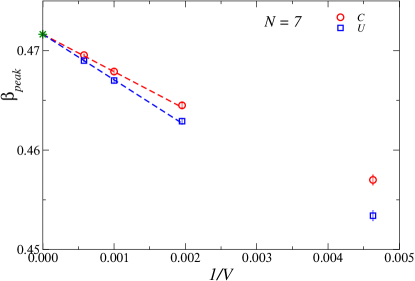
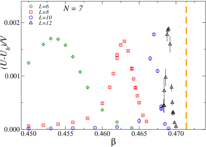
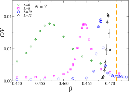
Figure 1: Estimates of the Binder cumulant $U$ (bottom left), of the specific heat (bottom right), and of the positions $\beta_{{\rm max},C}$ and $\beta_{{\rm max},U}$ of the maxima (top) for $N=7$. In the top panel we also report the extrapolations that provide an estimate of $\beta_{c}$.

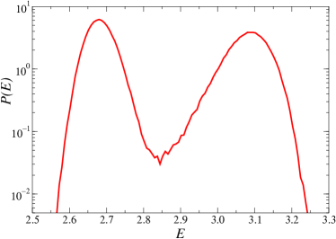
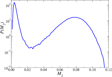
Figure 2: Distributions of the energy $E$ (left) and of $M_{2}=\mu_{2}/V^{2}$ (right), where $\mu_{2}$ is defined in Eq. (7) and $V$ is the volume. Results for $N=7$, $L=12$, $\beta=0.4693\approx\beta_{C,\rm max}(L)$.

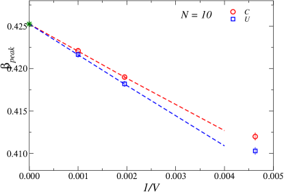
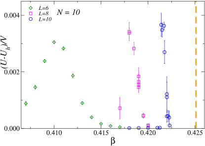
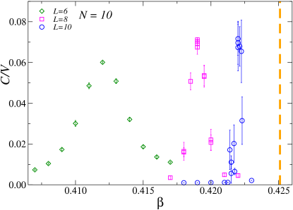
Figure 3: Estimates of the Binder cumulant $U$ (bottom left), of the specific heat (bottom right), and of the positions $\beta_{{\rm max},C}$ and $\beta_{{\rm max},U}$ of the maxima (top) for $N=10$. In the top panel we also report the extrapolations that provide an estimate of $\beta_{c}$.

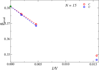
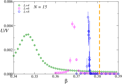
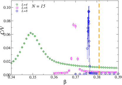
Figure 4: Estimates of the Binder cumulant $U$ (bottom left), of the specific heat (bottom right), and of the positions $\beta_{{\rm max},C}$ and $\beta_{{\rm max},U}$ of the maxima (top) for $N=15$. In the top panel we also report the extrapolations that provide an estimate of $\beta_{c}$.

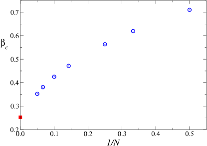
Figure 5: Plot of the available estimates of $\beta_{c}$ versus $1/N$. For $1/N=0$, we report $\beta_{c,\infty}\approx 0.25273$, which is probably a lower bound on the correct critical temperature for $N=\infty$ (see Sec. 3 for a discussion).

Table 1: Estimates at the transition point of the latent heat $\Delta_{h}$ and of the correlation lengths obtained from correlations of $Q$ [$\xi$, Eq. (6)], from the Polyakov loop [$\xi_{P}$, Eq. (12)] and from the gauge correlations $G_{V}(x)$ [$\xi_{z}$, Eq. (13)]. The suffix HT (LT) refers to the high-temperature (low-temperature, resp.) phase. The results for $\Delta_{h}$, $\xi_{HT}$ and $\xi_{z,HT}$ have been obtained on a lattice of size $L=24$, those for $\xi_{z,LT}$ on a lattice of size $L=48$ ($N=7$) or $L=40$ ($N=10,20$).

$N$	$\Delta_{h}$	$\xi_{HT}$	$\xi_{P,LT}$	$\xi_{z,HT}$	$\xi_{z,LT}$
7	0.4066(3)	1.710(6)	4.17(2)	1.46(1)	4.01(2)
10	0.5397(2)	1.169(5)		1.28(1)	5.22(5)
20	0.5806(2)	0.700(3)	6.71(2)	1.03(1)	6.95(20)

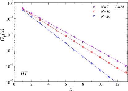
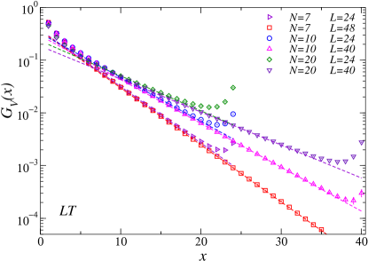
Figure 6: Plot of the correlation function $G_{V}(x)$ versus $x$, in the low-temperature (LT, bottom) and in the high-temperature phase (HT, top). Results at $\beta\approx\beta_{c}$ obtained starting the simulation from an ordered (LT) or disordered (HT) configuration. The dashed lines going through the points are fits to Eq. (13).

To analyze the behavior of the system in the two phases at $\beta\approx\beta_{c}$, we proceed as follows. We fix $\beta$ to our estimate of $\beta_{c}$ and perform two runs, which start from a disordered and an ordered configuration, respectively. If $L$ is large enough (as we discussed, it is enough to take $L\mathrel{\hbox to0.0pt{\lower 3.0pt\hbox{$\mathchar 536\relax$}\hss}\raise 2.0pt\hbox{$\mathchar 318\relax$}}16$), during the simulation there are no phase swaps and therefore, we are able to determine the average values of the different observables in the two phases. Using this method, we have estimated the average energy in the two phases and the corresponding latent heat. The results for $L=24$, reported in Table 1, are consistent with those that can be obtained from the behavior of the specific heat maximum, see Eq. (10). We have not attempted an infinite-volume extrapolatiom, but comparison with results for smaller values of $L$ indicates that size deviations are significantly less than 1%. The data show that $\Delta_{h}$ increases as $N$ increases: the first-order transition becomes stronger in the large-$N$ limit.

Similar conclusions are reached from the analysis of the correlations of the order parameter. In the low-temperature (LT) phase, $\xi$ computed from the $Q$ correlations, see Eq. (6), increases with $L$ for any $N$. This is of course expected, as the order parameter $Q$ condenses in the LT phase. On the other hand, in the HT phase, $\xi$ decreases with increasing $N$ and is always of order one. Apparently, correlations do not develop on the HT side of the transition as $N$ increases. This is obviously in contrast with the idea that the transition becomes continuous for large values of $N$. In this case, one would expect $\xi$ to increase with $N$, becoming of order $L$ for $N$ large enough, as expected in the vicinity of a critical transition.

To analyze the behavior of the gauge-field dependent observables, we first consider the Polyakov loop. Such a quantity is generically expected to decay exponentially with the system size [13], i.e.,

$$P(L)=A_{P}e^{-L/\xi_{P}},$$ (12)

with an appropriate correlation length $\xi_{P}$. In the HT phase, even for $L$ as small as 12, the Polyakov loop is negligible within errors (they are of the order of $10^{-5}$). If $A_{P}$ is a constant of order 1, this implies that $\xi_{P}$ is approximately 1 or smaller ($e^{-12}=6\cdot 10^{-6}$). In the HT phase, therefore, also gauge modes are essentially uncorrelated. In the LT phase, we can estimate $\xi_{P}$ considering data in the range $16\leq L\leq 40$. The results show that $\xi_{P}$ increases with $N$: gauge correlations become larger in the large-$N$ limit. Finally, we have considered the correlation function $G_{V}(x)$. As shown in Fig. 6, the curves behave quite precisely as exponentials, i.e., they are well fitted by

$$G_{V}(x)=Ae^{-x/\xi_{z}}.$$ (13)

If we fit the numerical results to Eq. (13), we obtain estimates of $\xi_{z}$ (they are reported in Table 1), that are consistent with a very simple scenario: gauge correlations are always negligible in the HT phase—for any $N$ and, therefore, also for $N\to\infty$—while in the LT phase they increase with $N$, leaving open the possibility that $\xi_{z}$ becomes infinite for $N\to\infty$.

Table 2: Estimates of the different correlation lengths as a function of $N$. In the second and third columns we report results obtained at $\beta=0.25273\approx\beta_{c,\infty}$, in the fourth and fifth column results for $\beta=0.8$. The HT results are obtained on lattices of size $L=16$; the LT estimates of $\xi_{z}$ on lattices with $L=24$ ($N=10,20$) and $L=32$ ($N=50,100$). The Polyakov correlation length is a fit of results with $16\leq L\leq 32$.

$N$	$\beta=0.25273$		$\beta=0.8$
	$\xi$	$\xi_{z}$	$\xi_{P}$	$\xi_{z}$
10	0.275(9)	0.70(1)		22.8(3)
20	0.285(5)	0.71(1)		47(3)
50	0.316(2)	0.72(1)	116.2(1)	116(10)
100	0.437(1)	0.87(2)	233.4(1)	225(20)

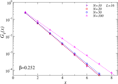
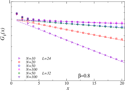
Figure 7: Plot of the correlation function $G_{V}(x)$ versus $x$, in the LT phase ($\beta=0.8$, bottom) and in the HT phase ($\beta=0.25273$, top), for different values of $N$. The dashed lines going through the points are fits to Eq. (13).

Summarizing, we have shown that, at least up to $N=20$, the model undergoes a first-order transition that apparently becomes stronger as $N$ increases. The transition separates two phases. The HT phase is disordered: both correlations of the order parameter $Q_{\bm{x}}$ and gauge correlations decay very rapidly, with a typical length scale of a lattice spacing. Moreover, the correlation lengths $\xi$ and $\xi_{x}$ apparently decrease as $N$ increases. In the LT phase the order parameter $Q_{\bm{x}}$ condenses and $\xi\sim L$. Gauge correlations are always massive, with a corresponding correlation length that increases with $N$. These results allow us to formulate a simple scenario for the behavior in the large-$N$ limit. We expect the $N=\infty$ transition to be of first order. For $\beta<\beta_{c}$ gauge and $Q$ correlations are always massive, while for $\beta>\beta_{c}$ both gauge-dependent vector correlations and gauge-invariant $Q$ correlations are massless: in the infinite-volume limit both $\xi$ and $\xi_{z}$ are infinite for $N=\infty$.

2.3 Phase behavior

Here we wish to provide additional support to the scenario discussed in the previous section, determining how $\xi$, $\xi_{P}$, and $\xi_{z}$ vary as a function of $N$ for two different fixed values of $\beta$. First, we consider $\beta=0.25273\approx\beta_{c,\infty}$, where $\beta_{c,\infty}$ is the transition point predicted by the large-$N$ analysis of [13]. If the standard large-$N$ analysis is correct, these runs should allow us to determine the behavior of the model on the HT side of the large-$N$ transition point. We will also perform runs at $\beta=0.8$, deep in the LT phase. We will consider four different values of $N$, $N=10,20,50,$ and 100.

Let us first consider the runs in the HT phase, at $\beta=0.25273$. Results for $L=16$ are reported in Table 2. For all values of $N$, $\xi$ is very small, consistent with a correlation of the order of at most one lattice spacing in the limit $N\to\infty$. A diverging correlation length for $N=\infty$ is clearly not consistent with the data. In Fig. 7 (top panel) we report the correlation function $G_{V}(x)$. It decays very rapidly with $x$ with a correlation length $\xi_{z}$ that is little dependent on $N$ and is always less than 1. We are unable to estimate the Polyakov correlation length, since the average of the Polyakov loop is always zero within errors ($10^{-5}$), as expected if $\xi_{P}\sim\xi_{z}\mathrel{\hbox to0.0pt{\lower 3.0pt\hbox{$\mathchar 536\relax$}\hss}\raise 2.0pt\hbox{$\mathchar 316\relax$}}1$. Again, data support the scenario that both gauge-invariant invariant modes associated with $Q_{{\bm{x}},\mu}$ and gauge modes are massive in the HT phase, even at the transition point, for any $N$, including $N=\infty$, consistently with an $N=\infty$ first-order transition.

The results in LT phase are also in agreement with the scenario reported in Sec. 2.2. The correlation length $\xi$ always scales with $L$ for any $N$, as expected. The correlation length $\xi_{z}$ is instead finite in the infinite-volume limit and apparently scales as $\xi_{z}\sim N$, a behavior which is also confirmed by the Polyakov correlation length $\xi_{P}$. Therefore, in the LT phase gauge modes are massive for any finite $N$ and become massless in the limit $N\to\infty$, consistently with what was observed on the LT side of the transition.

3 The large-$N$ standard solution: a critical discussion

The numerical data we have presented strongly suggest that the CP^N-1 model with Hamiltonian (2) undergoes a first-order transition for any $N>2$ and also for $N=\infty$. This is in contrast with [13] that predicted a continuous transition using some standard assumptions. We will now review the large-$N$ calculations, with the purpose of understanding which assumption is not correct. For the specific Hamiltonian (2), there is no need to use the general approach of [13]. One can obtain the same results in a more straighforward way, repeating on the lattice the same steps that are used in continuum calculations (see [9] and references therein). This simply amounts to trivially extending to three dimensions the lattice 2D calculations reviewed, for instance, in [17].

We start from the partition function, which can be written as

$$Z=\int\prod_{{\bm{x}}\mu}d\theta_{{\bm{x}}\mu}\,\prod_{\bm{x}}\left[d{\bm{z}}_{\bm{x}}d\bar{\bm{z}}_{x}\delta(\bar{\bm{z}}_{\bm{x}}\cdot{\bm{z}}_{\bm{x}}-1)\right]\,e^{-H},$$ (14)

where we wrote $\lambda_{{\bm{x}}\mu}=\exp(i\theta_{{\bm{x}}\mu})$. As usual, we write

$$\delta(\bar{\bm{z}}_{\bm{x}}\cdot{\bm{z}}_{\bm{x}}-1)={\beta N\over 2\pi i}\int_{c-i\infty}^{c+i\infty}d\gamma_{x}\exp[-\beta\gamma_{x}N(\bar{\bm{z}}_{\bm{x}}\cdot{\bm{z}}_{\bm{x}}-1)].$$ (15)

where $c$ is a real constant. We can then integrate over the $\bm{z}$-fields, obtaining

$$Z=(2\pi i)^{-V}\int\prod_{{\bm{x}}\mu}d\theta_{{\bm{x}}\mu}\prod_{\bm{x}}d\gamma_{\bm{x}}\,e^{-\beta NH_{\rm eff}},$$ (16)

where

$$H_{\rm eff}(\{\theta_{{\bm{x}}\mu},\gamma_{\bm{x}}\})={1\over 2}\hbox{Tr}\ \log(BB^{\dagger})+\sum_{\bm{x}}\gamma_{\bm{x}},$$ (17)

the matrix $B_{\bm{x}y}$ is given by

$$B_{\bm{x}y}=\gamma_{\bm{x}}\delta_{\bm{x}y}-e^{i\theta_{\bm{x}y}}\eta_{\bm{x}y},$$ (18)

and $\eta_{\bm{x}y}=1$ is equal to 1 if $x$ and $y$ are nearest neighbors and is zero otherwise.

The limiting behavior for $N\to\infty$ can be obtained by using the usual saddle-point method. For this purpose we must determine the stationary point of the effective Hamiltonian $H_{\rm eff}(\{\theta_{{\bm{x}}\mu},\gamma_{x}\})$ with the lowest (free) energy. In the usual approach one assumes that the relevant stationary point is obtained by considering translation invariant solutions of the gap equations. In other words, the saddle point is obtained by setting $\theta_{{\bm{x}}\mu}=\theta_{0}$ and $\gamma_{x}=\delta_{0}$, where $\theta_{0}$ and $\delta_{0}$ are constants independent of the position. Gauge invariance allows one to set $\theta_{0}=0$, implying that the saddle point corresponds to setting $\lambda_{{\bm{x}}\mu}=1$ on every link. Thus, the assumption of translation invariance essentially implies that the gauge variables play no role in the large $N$ limit (the same assumption is made in the continuum formulation, see, e.g., [9]). We thus obtain the effective Hamiltonian for the large-$N$ O($2N$) vector theory. One then predicts a continuous transition located at

$$\beta_{c,\infty}=\int{d^{3}p\over(2\pi)^{3}}{1\over\sum_{\mu}\hat{p}_{\mu}^{2}}\approx 0.25273,$$ (19)

where $\hat{p}=2\sin(p_{\mu}/2)$. In two dimensions, the assumption turns out to be correct, see [17] for a review. Our results show instead that this is not the case in three dimensions. The assumption that $\lambda_{{\bm{x}}\mu}=1$ on every link for $N=\infty$ is only correct in the LT phase. Indeed, in this phase we observe $1/\xi_{z},1/\xi_{P}\sim 1/N$, which confirms the existence of a massless gauge phase for $N=\infty$. In the HT phase, instead, even for $N$ strictly equal to infinity, gauge fields are spatially uncorrelated. This implies that, for small $\beta$, there is a different non-translation invariant saddle point with a lower free energy that gives the correct behavior of the theory.

As the HT phase is associated with a different saddle point of $H_{\rm eff}$, the critical point in the large-$N$ limit is not necessarily given by Eq. (19). However, the presence of a single transition, allows us to set the lower bound $\beta_{c}\geq\beta_{c,\infty}$. Indeed, in the opposite case, as the translation-invariant saddle point gives the solution for all values $\beta>\beta_{c}$, we would have a continuous transition for $\beta=\beta_{c,\infty}$, with a finite correlation length $\xi$ in the interval $\beta_{c}<\beta<\beta_{c,\infty}$. As there is no evidence of this intermediate phase, we conclude that $\beta_{c}\geq\beta_{c,\infty}$.

4 Conclusions

In this paper we have analyzed the phase diagram of the CP^N-1 model with Hamiltonian (2), with the objective of understanding the nature of the finite-temperature transition as a function of the number $N$ of components. The numerical data indicate that the transition is of first order. For all values of $N$ we consider, $N>2$ up to $N=100$, the correlation length $\xi$ obtained from correlations of the gauge-invariant order parameter $Q^{ab}$ defined in Eq. (3) is of order one on the HT side of the transition and diverges in the infinite-volume limit on the LT side. Moreover, the transition becomes stronger as $N$ increases: both the latent heat and the surface tension, which parametrize the free energy barrier between the two phases, increase with $N$. Vector and gauge correlations are massive for any finite $N$. On the HT side of the transition, the corresponding correlation lengths $\xi_{z}$ and $\xi_{P}$ are always of order one, for any value of $N$: gauge fluctuations are always uncorrelated, even for $N=\infty$. In the low-temperature phase, instead, we find that $\xi_{z},\xi_{P}\sim N$, so that gauge modes become massless in the large-$N$ limit.

Our results are consistent with a simple scenario in which, for any $N$ including $N=\infty$, the HT phase is always disordered, up to the transition point, where both correlations of the order parameter $Q$ and gauge correlations decay with a typical length scale of the order of one lattice spacing. In the LT phase, $Q$ condenses, while $\xi_{z},\xi_{P}\sim N$, so that for $N=\infty$ both gauge-invariant and gauge-dependent degrees of freedom are massless. The transition is therefore of first order, even for $N=\infty$.

These results contradict the analytic predictions of the many papers that investigated the large-$N$ limit, see, [18, 13] and references therein. The disagreement can be traced back to one of the standard assumptions which is used in the large-$N$ analysis, both for continuum and lattice models [17, 9, 18, 13]. In the calculation, one usually assumes that the relevant saddle point that controls the behavior of the large-$N$ free energy is translation invariant. For the gauge fields, this assumption implies that one can set $\lambda_{{\bm{x}},\mu}=1$ on any lattice link: gauge fields are assumed to play no role for $N=\infty$. Our results show that the assumption is correct in the LT phase, but fails in the HT phase: even for $N=\infty$ the gauge fields are disordered for any $\beta<\beta_{c}$. This is essentially consistent with the results of [21], that observed that hedgehog configurations forbid the ordering of gauge fields in the HT phase, at least if one takes the limit $N\to\infty$ before the limit $\xi\to\infty$.

The present results are in agreement with the predictions obtained in the so-called LGW approach defined in terms of the order parameter $Q^{ab}$, provided one assumes that the presence of a $\Phi^{3}$ term in the LGW Hamiltonian implies the absence of continuous transitions. It should be stressed that this assumption should not be taken for granted as it relies on an extrapolation of mean-field results to three dimensions. Note that, although we find no evidence of a large-$N$ critical transition, our results do not exclude it either, as it is a priori possible that our model is outside the attraction domain of this elusive fixed point.

It is interesting to compare our results with those of [3, 4, 5] for SU($N$) quantum antiferromagnets. Reference [3] studied a bilayer two-dimensional system and found a behavior analogous to what we find here. The transition is of first order for $N\geq 4$ and becomes stronger as $N$ increases from $N=4$ to $N=6$. On the other hand, for a single-layer two-dimensional system [4], an apparently continuous transition was always observed. The main difference between the two models is the topological nature of the allowed configurations. In the bilayer system, monopoles are allowed, while in the single-layer case monopoles are suppressed. In the model we consider, monopoles are allowed and we expect the transition to be characterized by their binding/unbinding: the monopole density should be positive in the HT phase and vanishing in the LT phase. Thus, on the basis of the results of [3, 4] and consistently with the discussion of [21], one may blame monopoles for the absence of a continuous transition. As the suppression of monopoles corresponds to adding an ordering interaction in the HT phase, it is conceivable—this would be consistent with the results of [4, 5]—that a continuous transition can be observed in a model in which monopoles are completely, or at least partially, suppressed. Clearly, additional work is needed to identify the role that monopoles play in the large-$N$ limit.

References

References

- [1] Read N and Sachdev S 1990 Spin-Peierls, valence-bond solid, and Néel ground states of low-dimensional quantum antiferromagnets Phys. Rev. B 42 4568
- [2] Takashima S, Ichinose I and Matsui T 2005 CP1+U(1) lattice gauge theory in three dimensions: Phase structure, spins, gauge bosons, and instantons Phys. Rev. B 72 075112
- [3] Kaul R K 2012 Quantum phase transitions in bilayer SU() antiferromagnets Phys. Rev. B 85 180411(R)
- [4] Kaul R K and Sandvik A W 2012 Lattice Model for the SU() Néel to Valence-Bond Solid Quantum Phase Transition at Large Phys. Rev. Lett. 108 137201
- [5] Block M S, Melko R G and Kaul R K 2013 Fate of CPN-1 fixed point with monopoles Phys. Rev. Lett. 111 137202
- [6] Motrunich O I and Vishwanath A 2004 Emergent photons and transitions in the O(3) sigma model with hedgehog suppression Phys. Rev. B 70 075104
- [7] Senthil T, Balents L, Sachdev S, Vishwanath S and Fisher M P A 2004 Quantum criticality beyond the Landau-Ginzburg-Wilson paradigm Phys. Rev. B 70 144407
- [8] Zinn-Justin J 2002 Quantum Field Theory and Critical Phenomena, fourth edition (Oxford:Clarendon Press)
- [9] Moshe M and Zinn-Justin J 2003 Quantum field theory in the large limit: A review Phys. Rep. 385 69
- [10] Pelissetto A and Vicari E 2019 Multicomponent compact Abelian-Higgs lattice models Phys. Rev. E 100 042134
- [11] Nahum A, Chalker J T, Serna P, Ortuño M and Somoza A M 2011 3D Loop Models and the CPN-1 Sigma Model Phys. Rev. Lett. 107 110601
- [12] Nahum A, Chalker J T, Serna P, Ortuño M and Somoza A M 2013 Phase transitions in three-dimensional loop models and the CPN-1 sigma model Phys. Rev. B 88 134411
- [13] Pelissetto A and Vicari E 2019 Three-dimensional ferromagnetic CPN-1 models Phys. Rev. E 100 022122
- [14] Halperin B I, Lubensky T C and Ma S K 1974 First-Order Phase Transitions in Superconductors and Smectic-A Liquid Crystals Phys. Rev. Lett. 32 292
- [15] Folk R and Holovatch Y 1996 On the critical fluctuations in superconductors J. Phys. A: Math. Gen. 29 3409
- [16] Ihrig B, Zerf N, Marquard P, Herbut I F and Scherer M M 2019 Abelian Higgs model at four loops, fixed-point collision and deconfined criticality Phys. Rev. B 100 134507
- [17] Campostrini M and Rossi P 1993 The expansion of 2-dimensional spin models Riv. Nuovo Cimento 16 1
- [18] Kaul R K and Sachdev S 2008 Quantum criticality of U(1) gauge theories with fermionic and bosonic matter in two spatial dimensions Phys. Rev. B 77 155105
- [19] Challa M S S, Landau D P and Binder K 1986 Finite-size effects at temperature-driven first-order transitions Phys. Rev. B 34 1841
- [20] Vollmayr K, Reger J D, Scheucher M and Binder K 1993 Finite size effects at thermally-driven first order phase transitions: A phenomenological theory of the order parameter distribution Z. Phys. B 91 113
- [21] Murthy G and Sachdev S 1990 Action of hedgehog-instantons in the disordered phase of the 2+1 dimensional CPN-1 model Nucl. Phys. B 344 557