Resonances in the Earth’s space environment

Abstract.

We study the presence of resonances in the region of space around the Earth. We consider a massless body (e.g, a dust particle or a small space debris) subject to different forces: the gravitational attraction of the geopotential, the effects of Sun and Moon. We distinguish different types of resonances: tesseral resonances are due to a commensurability involving the revolution of the particle and the rotation of the Earth, semi-secular resonances include the rates of variation of the mean anomalies of Moon and Sun, while secular resonances just depend on the rates of variation of the arguments of perigee and the longitudes of the ascending nodes of the perturbing bodies. We characterize such resonances, giving precise statements on the regions where the resonances can be found and provide examples of some specific commensurability relations.

1. Introduction

The dynamics of an object around the Earth has revealed many interesting aspects, thanks to the wide variety of behaviors occurring at different altitudes from the Earth. The space around our planet is usually split into three different regions, characterized by the acronyms LEO, MEO and GEO, where LEO stands for Low-Earth-Orbit ranging up to 2 000 km of altitude, MEO stands for Medium–Earth–Orbit between 2 000 and 30 000 km, GEO stands for Geostationary–Earth–Orbit. Objects in these regions feel different effects: Earth’s gravitational potential (including both the Keplerian part and the potential due to the non-spherical shape), gravitational influence of Sun and Moon, effect of Solar radiation pressure, dissipation due to the atmospheric drag (acting only in LEO), tides, or reradiation from the atmosphere. In this work we will not be concerned with the dynamics in LEO (which requires the analysis of the atmospheric drag), but we are rather concentrated on the analysis of orbits in MEO and GEO neglecting all non-conservative forces. Even more specifically, we focus on resonant motions occurring in MEO and GEO. Due to the high complexity of the system, there are several kinds of resonances, which involve the rates of variation of different variables associated to the object, Earth, Sun and Moon, each variable having its own time-scale.

More precisely, the angular variables associated to the dynamics of an object around the Earth are the mean motion, the argument of perigee and the longitude of the ascending node. Analogous variables are used to describe the dynamics of Sun and Moon, while the rotational motion of the Earth is described by the sidereal time. Associated to these variables, we have three different time scales:

$(i)_{t}$:

short periodic terms, involving the mean anomaly and the sidereal time, which are fast angles with periods of days;

$(ii)_{t}$:

semi-secular terms, involving the mean anomalies of Moon and/or Sun, which are semi-fast angles with periods of one month and one year;

$(iii)_{t}$:

secular terms, involving the arguments of perigee and the longitudes of the ascending nodes of the perturbers, which are slow angles with periods of several years.

As a consequence, we have a hierarchy of resonances, involving combinations of the angles evolving on different time scales: fast angles, like the mean motion of the object and the sidereal time of the Earth, slow angles, like the arguments of perigee or the longitudes of the ascending node (either of the object, Sun or Moon), intermediate angles (entering the semi-secular resonances), like the mean motions of the Moon or the Sun. We will give precise definitions in the following sections, but we anticipate here the terminology:

$(i)_{r}$:

tesseral resonances, occurring when there is a commensurability relation between the rates of variation of the mean motion of the object and of the sidereal time; such a relation will involve also the rates of variation of the argument of perigee and the longitude of the ascending node of the object;

$(ii)_{r}$:

Lunar or Solar semi-secular resonances, occurring when there is a commensurability relation between the rates of variation of the argument of perigee of the object, the longitude of the ascending node of the object, and the mean motion of the Moon or the Sun;

$(iii)_{r}$:

Lunar or Solar secular resonances, occurring when there is a commensurability relation between the rates of variation of the arguments of perigee and the longitudes of the ascending node of the object and the Moon, or the object and the Sun.

The most deeply investigated examples of resonances in the Earth’s space environment are the 1:1 and 2:1 tesseral resonances, where the orbital frequency of the object is equal or twice that of the Earth; in the 1:1 resonance we find geostationary satellites, while in the 2:1 resonance we find GPS satellites (see, e.g., [Alessi et al. (2018)], [Ely & Howell (1997)], [Gachet et al. (2017)], [Gkolias & Colombo (2019)], [Klinkrad (2006)], [Petit et al. (2018)], [Schettino et al. (2019)], [Skoulidou et al. (2018)]). The 1:1 and 2:1 resonances are located, respectively, at 42 164 km and 26 560 km from the center of the Earth.

Other tesseral resonances might be equally relevant for spacecraft operations, while lunisolar, semisecular and secular resonances, are important in designing disposal strategies. The study of resonances deserves much attention, especially in the context of space debris, which are small remnants of satellites, left in space after collisions, explosions or when a satellite becomes non-operative. Space debris represent a great threat due to the damages that their collision can provoke with operational or manned satellites.

Being covered by a web-like structure of resonances that induce various effects at different time scales, the circumterrestrial space is a dynamically complex environment. Inside resonance regions, the dynamical behavior of an uncontrolled object depends on the time scale at which the motion is studied and its initial position in the phase space. This remark motivates the need for a systematic classification of the different types of resonances, which manifest at different time scales, and a thorough investigation of their locations. Such a task involves explicit definitions and formulas for all constraints, a characterization of the main dynamical effects of resonances from the same category, a study of the location of resonances as a function of various parameters.

In this work we make a comprehensive investigation of the occurrences of the different kinds of resonances described in $(i)_{r}$-$(ii)_{r}$-$(iii)_{r}$ above. The natural tool is to adopt Hamiltonian formalism using a model that includes the geopotential (expanded in spherical harmonics and limited to a finite number of terms), the Lunar and Solar potentials. Within this setting, we give a characterization of the tesseral, Lunar and Solar semi-secular resonances, and Lunar and Solar secular resonances. In particular, we give results on the regions in the orbital elements space (semimajor axis, eccentricity and inclination) where the resonances can be found and how their location changes with the variation of the semimajor axis, eccentricity and inclination. We emphasize the fact that, even when large variations of the eccentricity and inclination induce only a small change in the location of the resonance, such a change may be important when compared to the size of the separatrices, dividing resonant and non-resonant kinds of motions in phase space. Moreover, we give a brief description of the main dynamical effects and phenomena of resonances from the same category. If tesseral resonances induce a variation of the semimajor axis on time scales of the order of hundreds of days, lunisolar resonances provoke variations of eccentricity and inclination on much longer time scales, of the order of tens or hundreds of years. The study of resonances depends, of course, on the (integer) values of the coefficients providing the resonance relation. The results of this work can be used as a guideline to study the geography of the different kinds of resonances, hence affecting the choice of the location of satellites or rather giving information on possible locations of disposal orbits.

This article is organized as follows. In Section 2 we describe the model (including the geopotential, Lunar and Solar disturbing functions) and we give the definitions of tesseral, semi-secular and secular resonances. The quadrupolar approximation is described in Section 3. The study of tesseral resonances is performed in Section 4, while semi-secular resonances are investigated in Section 5, and secular resonances are described in Section 6. Some conclusions are drawn in Section 7. A short survey of the chaos indicator used in this work (the Fast Lyapunov Indicator) is given in the Appendix.

2. The model and the resonances

We consider a massless body, say $S$, orbiting around the Earth in a region that includes both MEO and GEO; in our analysis, we do not include the LEO region in which the dissipative effect due to the atmospheric drag should be considered, thus changing the dynamics from conservative to dissipative. Moreover, we also neglect non-gravitational forces, like reradiation of the atmosphere, tides, the interaction with the Solar wind, or Solar radiation (acting also in GEO, see [Lhotka et al. (2016)]). We study the dynamics of $S$ under the effects of the oblateness of the Earth, and the Lunar and Solar attractions.

This study is accomplished by adopting the Hamiltonian formalism and by introducing the action–angle Delaunay variables, denoted as $(L,G,H,M,\omega,\Omega)$. We remind that the action variables $(L,G,H)$ are related to the orbital elements $(a,e,i)$ by the expressions

$$L=\sqrt{\mu_{E}a}\,,\qquad G=L\sqrt{1-e^{2}}\,,\qquad H=G\cos i\,,$$ (2.1)

where $a$ is the semimajor axis, $e$ the eccentricity, $i$ the inclination. As for the angle variables, the physical meaning is the following: $M$ is the mean anomaly, $\omega$ is the argument of perigee, $\Omega$ is the longitude of the ascending node. The quantity $\mu_{E}$ is equal to $\mu_{E}={\mathcal{G}}m_{E}$ with ${\mathcal{G}}$ the gravitational constant and $m_{E}$ the mass of the Earth. The orbital elements of the small body are referred to the celestial equator.

The corresponding Hamiltonian can be written as

$$\mathcal{H}=-{\mu^{2}_{E}\over{2L^{2}}}+\mathcal{H}_{Earth}(\Upsilon,\theta)-\mathcal{R}_{Sun}(\Upsilon,\Upsilon_{S})-\mathcal{R}_{Moon}(\Upsilon,\Upsilon_{M})\ ,$$ (2.2)

where $\theta$ denotes the sidereal time, we denote by $\Upsilon=(a,e,i,M,\omega,\Omega)$, $\Upsilon_{S}=(a_{S},e_{S},i_{S},M_{S},$ $\omega_{S},\Omega_{S})$, $\Upsilon_{M}=(a_{M},e_{M},i_{M},M_{M},\omega_{M},\Omega_{M})$ the orbital elements of the massless body, Sun and Moon, while $\mathcal{H}_{Earth}$, $\mathcal{R}_{Sun}$, $\mathcal{R}_{Moon}$ describe the perturbations due to the Earth, Sun and Moon, respectively.

2.1. The geopotential part

Denoting by $R_{E}$ the Earth’s radius, following [Kaula (1966)] we expand $\mathcal{H}_{Earth}$ as

$$\mathcal{H}_{Earth}=-{{\mu_{E}}\over a}\ \sum_{n=2}^{\infty}\sum_{m=0}^{n}\Bigl{(}{R_{E}\over a}\Bigr{)}^{n}\ \sum_{p=0}^{n}F_{nmp}(i)\ \sum_{q=-\infty}^{\infty}G_{npq}(e)\ S_{nmpq}(M,\omega,\Omega,\theta)\ ,$$ (2.3)

where the functions $F_{nmp}$, $G_{npq}$, $S_{nmpq}$ are given by classical relations ([Kaula (1966)]), which are given below for completeness. The expression of $F_{nmp}$ is given by

$$F_{nmp}(i) = \sum_{w}{{(2n-2w)!}\over{w!(n-w)!(n-m-2w)!2^{2n-2w}}}\sin^{n-m-2w}i\ \sum_{s=0}^{m}\left(\begin{array}[]{c}m\\ s\\ \end{array}\right)\cos^{s}i$$ (2.11)

$$\times\sum_{c}\left(\begin{array}[]{c}n-m-2w+s\\ c\\ \end{array}\right)\left(\begin{array}[]{c}m-s\\ p-w-c\\ \end{array}\right)(-1)^{c-k}\ ,$$

with $k=[{{n-m}\over 2}]$, $w$ is summed from zero to the $\min(p,k)$, $c$ is taken over all values such that the binomial coefficients are not identically zero. The expression for $G_{npq}$ is given by

$$G_{npq}(e)=(-1)^{|q|}(1+\beta^{2})^{n}\beta^{|q|}\ \sum_{k=0}^{\infty}P_{npqk}Q_{npqk}\beta^{2k}\ ,$$ (2.12)

where

$$\beta={e\over{1+\sqrt{1-e^{2}}}}\ ,$$

$$P_{npqk}=\sum_{r=0}^{h}\left(\begin{array}[]{c}2p^{\prime}-2n\\ h-r\\ \end{array}\right){{(-1)^{r}}\over r!}({{(n-2p^{\prime}+q^{\prime})e}\over{2\beta}})^{r}\ ,$$

with $h=k+q^{\prime}$ when $q^{\prime}>0$ and $h=k$ when $q^{\prime}<0$, and

$$Q_{npqk}=\sum_{r=0}^{h}\left(\begin{array}[]{c}-2p^{\prime}\\ h-r\\ \end{array}\right){1\over r!}({{(n-2p^{\prime}+q^{\prime})e}\over{2\beta}})^{r}\ ,$$

where $h=k$ when $q^{\prime}>0$ and $h=k-q^{\prime}$ when $q^{\prime}<0$, $p^{\prime}=p$ and $q^{\prime}=q$ when $p\leq n/2$, $p^{\prime}=n-p$ and $q^{\prime}=-q$ when $p>n/2$. The expression of $S_{nmpq}$ is given by

$$S_{nmpq}=\left[\begin{array}[]{c}C_{nm}\\ -S_{nm}\\ \end{array}\right]_{n-m\ odd}^{n-m\ even}\cos\Psi_{nmpq}+\left[\begin{array}[]{c}S_{nm}\\ C_{nm}\\ \end{array}\right]_{n-m\ odd}^{n-m\ even}\sin\Psi_{nmpq}\ ,$$ (2.13)

where

$$\Psi_{nmpq}=(n-2p)\omega+(n-2p+q)M+m(\Omega-\theta)\ .$$ (2.14)

We next introduce the coefficients $J_{nm}$ and the quantities $\lambda_{nm}$ so that

$$J_{nm}=\sqrt{C_{nm}^{2}+S_{nm}^{2}}\quad\textrm{if}\ m\neq 0\ ,\qquad J_{n0}\equiv J_{n}=-C_{n0}\ ,$$

$$C_{nm}=-J_{nm}\cos(m\lambda_{nm})\ ,\qquad S_{nm}=-J_{nm}\sin(m\lambda_{nm})\ .$$

With this notation, we can express $S_{nmpq}$ in the form

$$S_{nmpq}=\left\{\begin{array}[]{cc}-J_{nm}\cos\Psi_{nmpq}&\textrm{if}\ n-m\ \textrm{is even}\\ -J_{nm}\sin\Psi_{nmpq}&\textrm{if}\ n-m\ \textrm{is odd}\ .\\ \end{array}\right.$$

We remark that the Fourier series associated to $\mathcal{H}_{Earth}$ in (2.3) contains an infinite number of terms. Nevertheless, the long term variation of the orbital elements is governed by the secular and resonant terms. Moreover, we discussed in [Celletti & Galeş (2014)], [Celletti & Galeş (2018)] how to reduce the series to a finite number of terms, namely the terms which turn out to be the most relevant ones for the description of the dynamics.

We remark that the angle $\Psi_{nmpq}$ in (2.14) depends on linear combinations of different quantities, including the mean anomaly of the small particle and the sidereal time, hence there can occur resonances of the form

$$(n-2p+q)\dot{M}-m\dot{\theta}+(n-2p)\dot{\omega}+m\dot{\Omega}=0\ .$$ (2.15)

Setting $\ell=n-2p+q$ and $m=j$, we can re-write (2.15) as

$$\ell\ \dot{M}-j\ \dot{\theta}+j\ \dot{\Omega}+\ell\ \dot{\omega}-q\ \dot{\omega}=0\ .$$ (2.16)

Let us introduce the resonance angle

$$\sigma_{j\ell}=\ell\ M-j\ \theta+j\ \Omega+\ell\ \omega\ ,$$ (2.17)

so that (2.16) represents the rate of variation of

$$\sigma_{j\ell}-q\ \omega\ .$$ (2.18)

This discussion motivates the following definition.

Definition 1.

A tesseral resonance of order $j:\ell$ with $j$, $\ell\in{\mathbb{Z}}\backslash\{0\}$ occurs whenever the orbital period of the massless particle, the rotational period of the Earth, the rates of variation of the argument of perigee and the longitude of the ascending node of the massless particle satisfy the relation

$$\ell\ \dot{M}-j\ \dot{\theta}+j\ \dot{\Omega}+\ell\ \dot{\omega}=0\ ,\qquad j,\ell\in{\mathbb{Z}}\backslash\{0\}\ .$$ (2.19)

Remark 2.

We notice that for $J_{2}=0$, we have $\dot{\omega}=\dot{\Omega}=0$ (see (3) below); hence, the tesseral resonance reduces to a commensurability relation between the orbital period of the massless particle and the rotational period of the Earth, namely

$$\ell\ \dot{M}-j\ \dot{\theta}=0\ ,\qquad j,\ell\in{\mathbb{Z}}\backslash\{0\}\ .$$

For $q\not=0$, the term $q\ \dot{\omega}$ in (2.16) generates a multiplet of resonances ([Celletti & Galeş (2016b)]), thus leading to the following definition of multiplet tesseral resonance, that extends the Definition 1 of tesseral resonances.

Definition 3.

A multiplet tesseral resonance of order $j:\ell:q$ for $j,\ell,q\in{\mathbb{Z}}\backslash\{0\}$ occurs whenever the following relation is satisfied

$$\ell\ \dot{M}-j\ \dot{\theta}+j\ \dot{\Omega}+\ell\ \dot{\omega}-q\ \dot{\omega}=0\ .$$ (2.20)

Retaining only a finite number, say $N\in{\mathbb{Z}}_{+}$, of terms, we can approximate $\mathcal{H}_{Earth}$ by

$$\mathcal{H}_{Earth}=\mathcal{H}^{sec}_{Earth}+\mathcal{H}_{Earth}^{res}+\mathcal{H}_{Earth}^{nonres}\cong\sum_{n=2}^{N}\sum_{m=0}^{n}\sum_{p=0}^{n}\sum_{q=-\infty}^{\infty}\mathcal{T}_{nmpq}\ ,$$ (2.21)

where $\mathcal{H}^{sec}_{Earth}$, $\mathcal{H}_{Earth}^{res}$, $\mathcal{H}_{Earth}^{nonres}$ are the secular, resonant and non–resonant parts of the Earth’s potential ([Celletti & Galeş (2014)]); the sums have been truncated to a suitable finite order $N\in{\mathbb{Z}}_{+}$, and the coefficients $\mathcal{T}_{nmpq}$ are defined by:

$$\mathcal{T}_{nmpq}=-\frac{\mu_{E}R_{E}^{n}}{a^{n+1}}\ F_{nmp}(i)G_{npq}(e)S_{nmpq}(M,\omega,\Omega,\theta)\ .$$ (2.22)

2.1.1. The secular and resonant parts of the geopotential

The secular part of the geopotential expanded in (2.3) is obtained as the average over the fast angles $M$ and $\theta$.

Taking into account the expression of $S_{nmpq}$ in (2.13)-(2.14), we notice that the secular terms are those associated to the indexes $m=0$ and $n-2p+q=0$.

For our purposes, it will be convenient to approximate the secular part of (2.3) as ([Celletti & Galeş (2014)])

$${\color[rgb]{0,0,0}\mathcal{H}}_{Earth}^{sec} \cong \frac{\mu_{E}R^{2}_{E}J_{2}}{a^{3}}\Bigl{(}\frac{3}{4}\sin^{2}i-\frac{1}{2}\Bigr{)}(1-e^{2})^{-3/2}$$ (2.23)

$$+ \frac{2\mu_{E}R^{3}_{E}J_{3}}{a^{4}}\Bigl{(}\frac{15}{16}\sin^{3}i-\frac{3}{4}\sin i\Bigr{)}e(1-e^{2})^{-5/2}\sin\omega$$

$$+ \frac{\mu_{E}R^{4}_{E}J_{4}}{a^{5}}\Bigl{[}\Bigl{(}-\frac{35}{32}\sin^{4}i+\frac{15}{16}\sin^{2}i\Bigr{)}\frac{3e^{2}}{2}(1-e^{2})^{-7/2}\cos(2\omega)$$

$$+ \Bigl{(}\frac{105}{64}\sin^{4}i-\frac{15}{8}\sin^{2}i+\frac{3}{8}\Bigr{)}(1+\frac{3e^{2}}{2})(1-e^{2})^{-7/2}\Bigr{]}\ .$$

For the Earth, it turns out that $J_{2}\gg J_{n}$ for all $n\in\mathbb{N}$, $n>2$; hence, the most important harmonic of the secular Hamiltonian is that corresponding to $J_{2}$. When the expansion of $\mathcal{H}_{Earth}^{sec}$ is limited to the $J_{2}$ term, we will use the terminology of quadrupolar approximation of the Hamiltonian.

As for the resonant part of the geopotential, given the expressions (2.13)-(2.14) for the quantity $S_{nmpq}$, the terms corresponding to a tesseral resonance of order $j:\ell$ are those containing the angle $\sigma_{j\ell}$ as in (2.18) with $\ell=n-2p+q$ and $m=j$. The resonant part of the geopotential will then be a sum of terms with resonant arguments.

2.1.2. Solar and Lunar disturbing functions

The expressions for the Solar and Lunar disturbing functions are obtained as follows. We assume that the Solar elements, say $(a_{S},e_{S},i_{S},M_{S},\omega_{S},\Omega_{S})$, are referred to the equatorial frame ([Kaula (1962)]). We also assume that the Sun moves on a Keplerian ellipse with semimajor axis $a_{S}=1\,AU$, eccentricity $e_{S}=0.0167$, inclination $i_{S}=23^{\circ}26^{\prime}21.406^{\prime\prime}$, argument of perigee $\omega_{S}=282.94^{\circ}$, longitude of the ascending node $\Omega_{S}=0^{\circ}$; the rate of variation of the mean anomaly is assumed to be $\dot{M}_{S}\simeq 1^{\circ}/day$. Then, denoting by $m_{S}$ the mass of the Sun, the disturbing function due to the Sun can be written as

$$\mathcal{R}_{Sun} = \mathcal{G}m_{S}\sum_{l=2}^{\infty}\sum_{m=0}^{l}\sum_{p=0}^{l}\sum_{h=0}^{l}\sum_{q=-\infty}^{\infty}\sum_{j=-\infty}^{\infty}{a^{l}\over a_{S}^{l+1}}\ \epsilon_{m}\,{{(l-m)!}\over{(l+m)!}}$$ (2.24)

$$\times\ {\mathcal{F}}_{lmph}(i,i_{S})\mathcal{H}_{lpq}(e)\,\mathcal{G}_{lhj}(e_{S})\ \cos(\varphi_{lmphqj})\ ,$$

where

$${\mathcal{F}}_{lmph}(i,i_{S}) \equiv F_{lmp}(i)\ F_{lmh}(i_{S})\ ,$$

$$\varphi_{lmphqj} \equiv (l-2p)\omega+(l-2p+q)M-(l-2h)\omega_{S}-(l-2h+j)M_{S}+m(\Omega-\Omega_{S})\ ;$$

the quantities $\epsilon_{m}$ take the values

$$\epsilon_{m}=\left\{\begin{array}[]{cl}1&\text{if }m=0\ ,\\ 2&\text{if }m\in{\mathbb{Z}}\backslash\{0\}\ ,\end{array}\right.$$

the functions $\mathcal{H}_{lpq}(e)$ and $\mathcal{G}_{lhj}(e_{S})$ correspond to the Hansen coefficients $X_{l-2p+q}^{l,l-2p}(e)$, $X_{l-2h+j}^{-(l+1),l-2h}(e_{S})$, while $F_{lmp}(i)$ and $F_{lmh}(i_{S})$ are as in (2.11).

The contribution due to the Moon is conveniently formulated taking the elements of the satellite with respect to the equator and the elements of the Moon with respect to the ecliptic plane ([Lane (1989)]). With this choice, the inclination $i_{M}$ of the Moon is nearly constant, the rates of variation of the argument of perihelion $\omega_{M}$ of the Moon and that of the longitude of the ascending node $\Omega_{M}$ are nearly linear.

We assume that the Moon moves on a Keplerian ellipse with semimajor axis $a_{M}=384\,748\,km$, eccentricity $e_{M}=0.0549$ and inclination $i_{M}=5^{\circ}15^{\prime}$. Let $m_{M}$ be the mass of the Moon. Then, the Lunar disturbing function takes the form ([Celletti et al. (2017)], [Lane (1989)]):

$$\mathcal{R}_{Moon} = \mathcal{G}m_{M}\sum\limits_{l\geq 2}\sum\limits_{m=0}^{l}\sum\limits_{p=0}^{l}\sum\limits_{s=0}^{l}\sum\limits_{q=0}^{l}\sum\limits_{j=-\infty}^{+\infty}\sum\limits_{r=-\infty}^{+\infty}(-1)^{m+s}\ (-1)^{k_{1}}\frac{\epsilon_{m}\epsilon_{s}}{2a_{M}}\frac{(l-s)!}{(l+m)!}\left(\frac{a}{a_{M}}\right)^{l}$$

$$\times F_{lmp}(i)F_{lsq}(i_{M})\mathcal{H}_{lpj}(e)\mathcal{G}_{lqr}(e_{M})$$

$$\times \left\{(-1)^{k_{2}}U_{l}^{m,-s}\cos\left(\bar{\theta}_{lmpj}+\bar{\theta}_{lsqr}^{\prime}-y_{s}\pi\right)+(-1)^{k_{3}}U_{l}^{m,s}\cos\left(\bar{\theta}_{lmpj}-\bar{\theta}_{lsqr}^{\prime}-y_{s}\pi\right)\right\}\ ,$$

where $y_{s}=0$ for $s$ even, $y_{s}=1/2$ for $s$ odd, $k_{1}=[m/2]$, $k_{2}=t(m+s-1)+1$, $k_{3}=t(m+s)$ with $t=(l-1)$ mod 2, the terms $\bar{\theta}_{lmpj}$, $\bar{\theta}_{lsqr}^{\prime}$ are given by

$$\bar{\theta}_{lmpj} = (l-2p)\omega+(l-2p+j)M+m\Omega\ ,$$

$$\bar{\theta}_{lsqr}^{\prime} = (l-2q)\omega_{M}+(l-2q+r)M_{M}+s(\Omega_{M}-\pi/2)\ ,$$

the functions $U_{l}^{m,s}$ have the following expressions (compare with [Celletti et al. (2017)])

$$U_{l}^{m,s} = \sum_{r=\max(0,-(m+s))}^{\min(l-s,l-m)}(-1)^{l-m-r}\left(\begin{array}[]{c}l+m\\ m+s+r\\ \end{array}\right)\ \left(\begin{array}[]{c}l-m\\ r\\ \end{array}\right)\ \cos^{m+s+2r}({\varepsilon\over 2})\sin^{-m-s+2(l-r)}({\varepsilon\over 2})\ ,$$

where $z=\cos^{2}({\varepsilon\over 2})$ and $\varepsilon$ denotes the obliquity of the ecliptic. The functions $\mathcal{H}_{lpj}(e)$ and $\mathcal{G}_{lqr}(e_{S})$ represent the Hansen coefficients $X_{l-2p+j}^{l,l-2p}(e)$, $X_{l-2q+r}^{-(l+1),l-2q}(e_{M})$.

Given the expansions above of the Solar and Lunar perturbing functions, we are led to introduce the following definitions of Solar and Lunar secular resonances.

Definition 4.

A Solar gravity secular resonance occurs whenever there exists an integer vector $(k_{1},k_{2},k_{3},k_{4})\in{\mathbb{Z}}^{4}\backslash\{0\}$, such that

$$k_{1}\dot{\omega}+k_{2}\dot{\Omega}+k_{3}\dot{\omega}_{S}+k_{4}\dot{\Omega}_{S}=0\ .$$ (2.27)

A Lunar gravity secular resonance occurs whenever there exists an integer vector $(k_{1},k_{2},k_{3},k_{4})\in{\mathbb{Z}}^{4}\backslash\{0\}$, such that

$$k_{1}\dot{\omega}+k_{2}\dot{\Omega}+k_{3}\dot{\omega}_{M}+k_{4}\dot{\Omega}_{M}=0\ .$$ (2.28)

We stress that the above definition of secular resonances is as general as possible. However, given the fact that we will consider Solar and Lunar expansions truncated to the second order in the ratio of the semi–major axes, in view of (2.24) and (2.1.2), the Hamiltonian ${\mathcal{H}}$ is independent of $\omega_{M}$ and $\omega_{S}$. Therefore, for all resonances studied here, one has $k_{3}=0$. Moreover, since $\dot{\Omega}_{S}\simeq 0$, the relations (2.27) and (2.28) may be rewritten in the particular form:

$$(2-2p)\dot{\omega}+m\dot{\Omega}=0\ ,\qquad m,p=0,1,2\,,$$

and

$$(2-2p)\dot{\omega}+m\dot{\Omega}+\kappa\dot{\Omega}_{M}=0\ ,\qquad m,p=0,1,2,\quad\kappa=-2,-1,0,1,2\,,$$

respectively.

According to the classification of the harmonic terms of the expansions (2.24) and (2.1.2), we define the Solar and Lunar semi–secular resonances as follows (compare with [Hughes (1980)]).

Definition 5.

A Solar semi–secular resonance occurs whenever

$$(l-2p)\dot{\omega}+m\dot{\Omega}-(l-2h+j)\dot{M}_{S}=0\ ,\qquad l\in\mathbb{Z}_{+}\,,\ m,p,h=0,1,2,...,l\,,\ j\in\mathbb{Z}.$$

We have a Lunar semi–secular resonance whenever

$$(l-2p)\dot{\omega}+m\dot{\Omega}\pm[(l-2q)\dot{\omega}_{M}+(l-2q+r)\dot{M}_{M}+s\dot{\Omega}_{M}]=0\ ,$$

$$\qquad\qquad\qquad\qquad\qquad\qquad\qquad\qquad\ l\in\mathbb{Z}_{+}\,,\ m,p,q,s=0,1,2,...,l\,,\ r\in\mathbb{Z}.$$

By taking a quadrupolar approximation of the expansions (2.24) and (2.1.2), namely considering $l=2$, it follows that the possible resonances have the form:

$$\alpha\dot{\omega}+\beta\dot{\Omega}-\gamma\dot{M}_{S}=0\ ,\qquad\alpha\in\{\pm 2,0\}\,,\quad\beta\in\{\pm 2,\pm 1,0\}\,,\quad\gamma\in\mathbb{Z}\backslash\{0\}$$

for the Sun and

$$\begin{split}&\alpha\dot{\omega}+\beta\dot{\Omega}+\alpha_{M}\dot{\omega}_{M}+\beta_{M}\dot{\Omega}_{M}-\gamma\dot{M}_{M}=0\ ,\qquad\alpha\,,\alpha_{M}\in\{\pm 2,0\}\,,\\ &\hskip 199.16928pt\beta,\beta_{M}\in\{\pm 2,\pm 1,0\},\quad\gamma\in\mathbb{Z}\backslash\{0\}\end{split}$$

for the Moon. We remark that Lunar semi–secular resonances occur at very low altitudes and therefore their interest is limited.

3. Quadrupolar approximation

The quadrupolar approximation is obtained by summing the Keplerian part $-\mu_{E}^{2}/(2L^{2})$ and the secular part (namely, the term of the series (2.21) for which $n=2$, $m=0$, $p=1$, $q=0$). Since $F_{201}(i)=0.75\sin^{2}i-0.5$ and $G_{210}(e)=(1-e^{2})^{-3/2}$ (see (2.11) and (2.12)), from (2.23) we obtain the Hamiltonian

$${\mathcal{H}}_{Kepler+J_{2}}=-\frac{\mu_{E}^{2}}{2L^{2}}+{{R_{E}^{2}J_{2}\mu_{E}^{4}}\over{4}}\ {{1}\over{L^{3}G^{3}}}\ \Bigl{(}1-3{H^{2}\over G^{2}}\Bigr{)}\ .$$ (3.1)

Since the angles in ${\mathcal{H}}_{Kepler+J_{2}}$ are ignorable, it follows that $L$, $G$ and $H$ are constant, while the Delaunay angle variables $M$, $\omega$ and $\Omega$ evolve linearly in time with rates of variation:

$$\dot{M} = \frac{\mu_{E}^{2}}{L^{3}}-\frac{3R_{E}^{2}J_{2}\mu_{E}^{4}}{4}\frac{1}{L^{4}G^{3}}\Bigl{(}1-3\frac{H^{2}}{G^{2}}\Bigr{)}\,,$$

$$\dot{\omega} = \frac{3R_{E}^{2}J_{2}\mu_{E}^{4}}{4}\frac{1}{L^{3}G^{4}}\Bigl{(}-1+5\frac{H^{2}}{G^{2}}\Bigr{)}\,,$$

$$\dot{\Omega} = -\frac{3R_{E}^{2}J_{2}\mu_{E}^{4}}{2}\frac{H}{L^{3}G^{5}}\ .$$ (3.2)

By using the following data: $m_{E}=5.972\cdot 10^{24}$ $kg$, ${\mathcal{G}}=6.67408\cdot 10^{-11}$ $m^{3}/(kg\,s^{2})$, $R_{E}=6378.137\cdot 10^{3}$ $m$, $J_{2}=1082.6261\cdot 10^{-6}$, and using the conversion factor $60\cdot 60\cdot 24\cdot 360/(2\pi)$, one obtains that

$${{({\mathcal{G}}m_{E})^{1\over 2}}\over{R_{E}^{3\over 2}}}=6135.7^{o}/day\ ,\qquad{{3J_{2}({\mathcal{G}}m_{E})^{1\over 2}}\over{4R_{E}^{3\over 2}}}=4.98^{o}/day\ .$$

Hence, we can approximate the relations (3) in terms of the orbital elements as:

$$\begin{split}&\dot{M}\simeq 6135.7\Bigl{(}\frac{R_{E}}{a}\Bigr{)}^{3/2}-4.98\Bigl{(}\frac{R_{E}}{a}\Bigr{)}^{7/2}(1-e^{2})^{-3/2}(1-3\cos^{2}i)\ ^{o}/day\,,\\ &\dot{\omega}\simeq 4.98\Bigl{(}\frac{R_{E}}{a}\Bigr{)}^{7/2}(1-e^{2})^{-2}(5\cos^{2}i-1)\ ^{o}/day\,,\\ &\dot{\Omega}\simeq-9.97\Bigl{(}\frac{R_{E}}{a}\Bigr{)}^{7/2}(1-e^{2})^{-2}\cos i\ ^{o}/day\,.\\ \end{split}$$ (3.3)

Therefore, we are led to summarize as follows the main effects of $J_{2}$: a slow change of the rate of the mean anomaly, a precession of the perigee and a secular regression of the orbital node.

Our results can be generalized to higher orders in a straightforward way: let us write the quadrupolar Hamiltonian in compact form as

$${\color[rgb]{0,0,0}\mathcal{H}}_{Q}=-{{\mu_{E}^{2}}\over{2L^{2}}}+J_{2}\ F_{2}(L,G,H)$$

for a suitable function $F_{2}$ whose expression can be obtained from (3.1). If we include other spherical harmonic coefficients, e.g. $J_{3}$ and $J_{4}$, pertaining to the secular part of the Hamiltonian, we are led to add to ${\color[rgb]{0,0,0}\mathcal{H}}_{Q}$ terms of the form

$${\color[rgb]{0,0,0}\mathcal{H}}_{add}=J_{3}\ F_{3}(L,G,H,\omega)+J_{4}\ F_{4}(L,G,H,\omega)$$

for suitable functions $F_{3}$ and $F_{4}$. Hence, for the new system the rate of variation of the mean anomaly is given by

$$\dot{M}={{\partial({\color[rgb]{0,0,0}\mathcal{H}}_{Q}+{\color[rgb]{0,0,0}\mathcal{H}}_{add})}\over{\partial L}}\ ,$$

which makes $\dot{M}$ depending also on $\omega$. This might generate a superposition of resonances and, therefore, a characterization of chaos in a model which is not just the quadrupolar approximation.

4. A characterization of tesseral resonances

In this Section we study tesseral resonances, which involve the rates of variation of the mean anomaly of the object, the rate of the sidereal time and the rates of variation of the argument of perigee and the longitude of the ascending node of the object. The main results of this Section are the following: in Proposition 7 we fix $a$, $e$ and find that the resonance relation gives an expression for the inclination; in Proposition 8 we fix $e$, $i$ and find an equation for the semimajor axis; in Proposition 9 we fix $a$, $i$ and find an expression for the eccentricity.

Within the quadrupolar approximation, using (LABEL:MomeagaOmega_var) a tesseral resonance of order $j:\ell$, $j,\ell\in{\mathbb{Z}}\backslash\{0\}$, occurs whenever the semimajor axis, eccentricity and inclination satisfy the following relation:

$$\Big{\{}\ell\ \Big{[}6135.7({R_{E}\over a})^{3\over 2}-4.98({R_{E}\over a})^{7\over 2}(1-e^{2})^{-{3\over 2}}(1-3\cos^{2}i)+4.98({R_{E}\over a})^{7\over 2}(1-e^{2})^{-2}(5\cos^{2}i-1)\Big{]}$$

$$-j\ 9.97({R_{E}\over a})^{7\over 2}(1-e^{2})^{-2}{\color[rgb]{0,0,0}\cos i}\Big{\}}\ {1\over{360}}\ {365.242196\over{366.242196}}=j\ ,$$

where the factor $365.242196/366.242196$ is introduced to transform from mean Solar to sidereal days.

Remark 6.

We notice that if $J_{2}=0$, then $\dot{\omega}=\dot{\Omega}=0$ and the first in (3) reduces to

$$\dot{M}=6135.7\ ({R_{E}\over a})^{3\over 2}\ .$$

Hence, tesseral resonances can occur for any inclination and eccentricity, provided the semimajor axis satisfies the relation

$$6135.7\ ({R_{E}\over a})^{3\over 2}\ {1\over{360}}\ {{365.242196}\over{366.242196}}={j\over\ell}\ .$$

Therefore, the effect of $J_{2}$ is to introduce a dependence of the tesseral resonances on eccentricity and inclination as well as a precession of $\omega$ and $\Omega$.

The following result provides the condition under which the inclination satisfies a tesseral resonance of order $j:\ell$, whenever the semimajor axis and eccentricity are fixed.

Proposition 7.

Within the quadrupolar approximation (3.1), for a fixed value of $a$ and $e$, denoting by $A$, $B$, $C$, $\tau$ the quantities

$$A = 6135.7({R_{E}\over a})^{3\over 2}-4.98({R_{E}\over a})^{7\over 2}(1-e^{2})^{-{3\over 2}}-4.98({R_{E}\over a})^{7\over 2}(1-e^{2})^{-2}\ ,$$

$$B = 14.94({R_{E}\over a})^{7\over 2}(1-e^{2})^{-{3\over 2}}+24.90({R_{E}\over a})^{7\over 2}(1-e^{2})^{-2}\ ,$$

$$C = 9.97({R_{E}\over a})^{7\over 2}(1-e^{2})^{-2}\ ,$$

$$\tau = {{365.242196}\over{366.242196}}\ ,$$

a tesseral resonance of order $j:\ell$ occurs for values of the inclination such that

$$\cos i=\frac{C\ j\pm\sqrt{C^{2}\ j^{2}-4B\ell\left(\ell A-360\ j/\tau\right)}}{2B\ell}\ ,$$

provided the following conditions are satisfied:

$$C^{2}\ j^{2}-4B\ell\left(\ell A-360\ j/\tau\right)\geq 0\ ,$$

$$\Bigl{|}\frac{C\ j\pm\sqrt{C^{2}\ j^{2}-4B\ell\left(\ell A-360\ j/\tau\right)}}{2B\ell}\Bigr{|}\leq 1\ .$$

The proof of Proposition 7, as well as those of Propositions 8 and 9 below, is elementary, since it suffices to insert in Definition 1 the value for $\dot{M}$ in (LABEL:MomeagaOmega_var).

If we fix the eccentricity and the inclination, we obtain the following solutions for the semimajor axis.

Proposition 8.

Within the quadrupolar approximation (3.1), for a fixed value of $e$ and $i$, denoting by $A$, $B$, $C$, $\rho$ the quantities

$$A = 6135.7\ ,$$

$$B = 4.98(1-e^{2})^{-{3\over 2}}\ (1-3\cos^{2}i){\color[rgb]{0,0,0}-}4.98(1-e^{2})^{-2}\ (5\cos^{2}i-1)\ ,$$

$$C = 9.97(1-e^{2})^{-2}{\color[rgb]{0,0,0}\cos{\left(i\right)}}\ ,$$

$$\rho = \Bigl{(}{R_{E}\over a}\Bigr{)}^{1\over 2}\ ,$$

$${\color[rgb]{0,0,0}\tau} = {\color[rgb]{0,0,0}{{365.242196}\over{366.242196}}}\ ,$$

a tesseral resonance of order $j:\ell$ occurs for values of the semimajor axis such that

$$\ell\ A\rho^{3}-(\ell B+jC)\rho^{7}={360\over\tau}j\ .$$

Finally, if we fix the semimajor axis and the inclination, we obtain the following result for the eccentricity.

Proposition 9.

Within the quadrupolar approximation (3.1), for a fixed value of $a$ and $i$, denoting by $\varepsilon$, $A$, $B$, $C$, $D$, the quantities

$${\color[rgb]{0,0,0}\varepsilon} = (1-e^{2})^{-1}\ ,$$

$$A = 6135.7({R_{E}\over a})^{3\over 2}\ ,$$

$$B = 4.98({R_{E}\over a})^{7\over 2}\ (1-3\cos^{2}i)\ ,$$

$$C = 4.98({R_{E}\over a})^{7\over 2}\ (5\cos^{2}i-1)\ ,$$

$$D = 9.97({R_{E}\over a})^{7\over 2}{\color[rgb]{0,0,0}\cos i}\ ,$$

$${\color[rgb]{0,0,0}\tau} = {\color[rgb]{0,0,0}{{365.242196}\over{366.242196}}}\ ,$$

a tesseral resonance of order $j:\ell$ occurs for values of the eccentricity (namely of $\varepsilon$) which are solutions of the following equation:

$$(jD-\ell C)\varepsilon^{2}+\ell B\varepsilon^{3\over 2}+({{360}\over\tau}j-\ell A)=0\ .$$

The dependency of the location of $j:\ell$ resonances on the orbital parameters is shown in Figure 1. The grey shaded regions provide the values in which (4) can be solved, contours are marked for different values of orbital parameters as shown in the plot legends at the top. The value of the semi-major axis $a$ weakly depends on the choice of $e$ and $i$. In Figure 1 the values $a_{geo}$ and $a_{0}$ denote the nominal values of the semimajor axes corresponding, respectively, to the 1:1 and 5:1 resonances, when the oblateness, the eccentricity, and the inclination are set to zero. As Figure 1 shows, the deviations from the nominal values are less than $10$ km, and they are higher when increasing the order of the resonance.

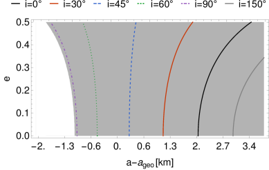
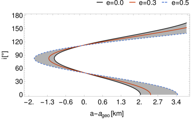
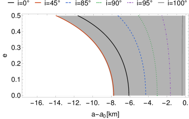
Figure 1. Location of tesseral resonances in $(a,e)$-space (left) and $(a,i)$-space (right) for the $1:1$ (top) and the $5:1$ resonances (bottom). Values on abscissae are deviations from the reference value (defined as $J_{2}=e=i=0$) given in $km$.

The dependency of the location of the resonance on the $J_{2}$ gravity field expansion coefficient is shown in Table 1. The influence of the flattening of the Earth on the resonant value of the semi-major axis $a$ ranges from less than 1 km (resonances $3:4$) up to a few kilometers, e.g. for the resonance $5:1$.

$$\begin{array}[]{|c|c|r|r|c|}\hline\cr\hline\cr j&\ell&a_{J_{2}}[km]&a[km]&a_{J_{2}}-a[km]\\ \hline\cr 3&4&51\ 079.116&51\ 078.254&0.860\\ 4&5&48\ 928.085&48\ 927.185&0.900\\ 1&1&42\ 165.214&42\ 164.170&1.044\\ 5&4&36\ 337.192&36\ 335.980&1.212\\ 4&3&34\ 807.020&34\ 805.755&1.265\\ 3&2&32\ 178.652&32\ 177.284&1.369\\ 5&3&29\ 996.159&29\ 994.691&1.468\\ 2&1&26\ 563.420&26\ 561.762&1.658\\ 5&2&22\ 892.157&22\ 890.233&1.924\\ 3&1&20\ 272.591&20\ 270.419&2.172\\ 4&1&16\ 735.493&16\ 732.862&2.631\\ 5&1&14\ 422.996&14\ 419.943&3.053\\ \hline\cr\end{array}$$

Table 1. Values of $j:\ell$ tesseral resonances with ($a_{J_{2}}$) and without ($a$) the dependency on $J_{2}$.

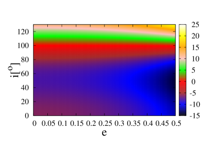
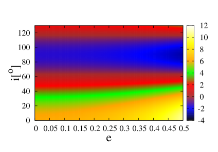
Figure 2. Resonance 5:1. Shift in semi–major axis (color bar in km) of the location of the equilibria as a function of $e$ and $i$, due to the effect of $J_{2}$. Left: Shift of the location of the exact resonance $\dot{\sigma}_{51}=0$ from the nominal value $a_{5:1}=14\,419.9\$ km (see also the Table 1). Right: Shift of the location of the exact resonance of a harmonic term whose argument is $\sigma_{51}+(k+1)\omega$, $k\in\mathbb{Z}$, from the location of the resonance associated to another harmonic term whose argument is $\sigma_{51}+k\omega$.

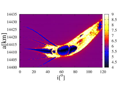
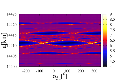
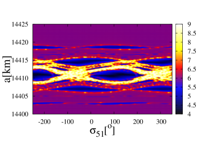
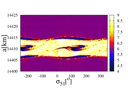
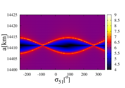
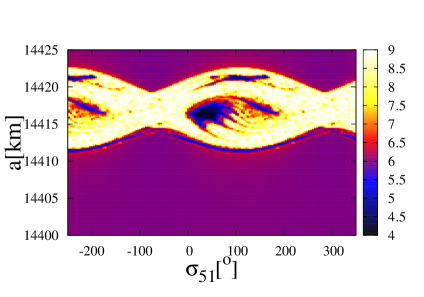
Figure 3. FLI for the 5:1 tesseral resonance as a function of semi-major axis and inclination (top left) and respectively semi-major axis and resonant angle (all other plots). The initial values are $e=0.3$, $\omega=0^{o}$, $\Omega=0^{o}$ for all panels. The top left panel is obtained for the initial resonant angle $\sigma_{51}=105^{o}$, while the plots in the $(a-\sigma_{51})$–plane are computed for $i=32^{o}$ (top right), $i=38^{o}$ (middle left), $i=50^{o}$ (middle right), $i=63.4^{o}$ (bottom left) and $i=90^{o}$ (bottom right).

Due to the effect of the secular part, the frequencies $\dot{\omega}$ and $\dot{\Omega}$ are not zero (compare with $\eqref{MomeagaOmega_var}$). As a consequence, as already pointed out in Definition 3, each $j:\ell$ resonance splits into a multiplet of resonances and, hence, each harmonic term of a specific resonance, with big enough magnitude, yields equilibria located at different distances from the center of the Earth. Roughly speaking, the values provided in Table 1 give just a hint on the location of the resonances, including the minor ones, different from 1:1 and 2:1. Actually, the location and width of the minor resonances, as well as the regular and chaotic behavior of the corresponding resonant regions, are affected by the interaction between the secular part and the resonant harmonic terms. The dynamics of a $j:\ell$ tesseral resonance may be analytically described by estimating the location of the equilibria of specific components of the multiplet and the width of the associated resonant islands.

Thus, when studying a tesseral resonance, by using (LABEL:MomeagaOmega_var) we can estimate the location of the exact resonance for each component of the multiplet (2.20). For example, Figure 2 provides the shift of the equilibria from the nominal value $a_{5:1}=14\,419.9\,km$, expressed in kilometers, as a function of eccentricity and inclination, for the $5:1$ resonance. Let us recall the definition $\sigma_{j\ell}\equiv\ell M-j\theta+\ell\omega+j\Omega$. The left panel of Figure 2 shows the shift of the location of the equilibria associated to the exact resonance $\dot{\sigma}_{51}=0$ from the nominal distance $a_{5:1}=14\,419.943\ km$, given in Table 1 and obtained by using Kepler’s third law. Negative values are used to show that the equilibria are closer to the Earth than $a_{5:1}$, while positive values are used to express that the equilibria are farther from the Earth than $a_{5:1}$. The right panel gives the shift of the location of the exact resonance of a harmonic term whose argument is $\sigma_{51}+(k+1)\omega$, $k\in\mathbb{Z}$, from the location of the resonance associated to another harmonic term whose argument is $\sigma_{51}+k\omega$. We recall that $\sigma_{51}$ denotes the resonant angle $\sigma_{51}=M-5\theta+\omega+5\Omega$. The positive/negative sign in the color bar expresses the fact that the equilibrium point associated to the term whose argument is $\sigma_{51}+(k+1)\omega$ is located farther/closer to the Earth than the equilibrium point corresponding to the harmonic term whose argument is $\sigma_{51}+k\omega$.

By using Figure 2 in connection with a simple procedure for computing the amplitude of the resonant island for a specific multiplet, as described in [Celletti & Galeş (2015)], we can give an analytical explanation concerning the location of the equilibrium points, an estimate of the amplitude of the resonant island (or islands) and a description of the dynamics of space debris in the resonant regions for each tesseral resonance.

Analyzing the right panel of Figure 2, and taking also into account that the amplitude of the resonant islands is of the order of few kilometers, we can infer that for small inclinations a splitting phenomenon takes place, namely the width of the resonance associated to each component of the multiplet is smaller than the distance separating these resonances. On the contrary, for larger inclinations we have an opposite phenomenon, called superposition of harmonics, which gives rise to a complex behavior of the semi-major axis. Indeed, Figure 3 shows a cartography of the 5:1 tesseral resonance in the $(a,i)$–plane (top left) and in the $(a-\sigma_{51})$–plane (all other plots), for eccentricity $e=0.3$ based on the computation of Fast Lyapunov Indicators (hereafter FLIs, see the Appendix for more details on the tools used to study the cartography of the resonances). Thus, for $i<35^{o}$ it is easy to see that the amplitude of the resonant islands vary from 0 to 4 kilometers (compare with [Celletti & Galeş (2015)]), while the minimum distance between the equilibria associated to any two harmonic terms is larger than 4 kilometers (see the top right panel of Figure 2). Therefore, the harmonic terms having large enough magnitude give rise to non–overlapping resonances, as shown by the top right panel of Figure 3. The situation is opposite for larger inclinations, say $i>35^{o}$ (with the exception of the value $i=63.4^{o}$ corresponding to the critical inclination and discussed below), at least for moderate eccentricities (that is $e\in[0.15,0.5])$; the width of the resonant island associated to the dominant term, which in this case is $\mathcal{T}_{5520}$, is at least 4 kilometers, while Figure 2 (top right) shows that it is possible to have harmonic terms $\mathcal{T}_{nmpq}$ whose associated equilibria are shifted by less than 4 kilometers. If these terms are comparable in magnitude with the dominant term (most of them satisfy this assumption, provided the eccentricity is large enough as in Figure 3), then the resonances of the multiplet superimpose (middle left, middle right and bottom right of Figure 3).

Let us remark that for any resonance an interesting fact occurs at the critical inclination $i=63.4^{o}$. Within the $J_{2}$ approximation, this value of the inclination makes the argument of perigee to be constant (see relation $\eqref{MomeagaOmega_var}$) and since the argument of any two harmonic terms differs by $k\omega$, then the shift in $a$ is zero. As a result, for $i=63.4^{o}$ the pattern of the resonance is similar to a pendulum (see bottom left panel of Figure 3).

5. A characterization of semi-secular resonances

In this Section we give some results for the semi-secular resonances associated to the effects of Sun (Sections 5.1 and 5.2) and Moon (Section 5.3). The Solar semi-secular resonances involve the rates of variation of the argument of perigee, the longitude of the ascending node and the Sun’s mean motion. We consider different cases within the quadrupolar approximation: in Proposition 10 we fix $a$, $e$ and obtain a constraint on the inclination; in Proposition 11 we fix $e$, $i$ and find an expression for the semimajor axis; in Proposition 12 we fix $a$, $i$ and find an expression for the eccentricity. A model for the description of the dynamics in the neighborhhod of the Solar semi-secular resonances is introduced in Section 5.2. Lunar semi-secular resonances are discussed in Section 5.3; in particular, we give bounds for the existence of solutions when $a$, $e$ are fixed (Proposition 13), for a given semimajor axis and $e$, $i$ satisfying a constraint (Proposition 14), for a given eccentricity and $a$, $i$ satisfying a constraint (Proposition 15).

5.1. Solar semi-secular resonances

Solar semi-secular resonances are characterized by a relation of the form

$$\alpha\dot{\omega}+\beta\dot{\Omega}-\gamma\dot{M}_{S}=0\ ,$$ (5.1)

where $\alpha=0,\pm 2$, $\beta=0,\pm 1,\pm 2$, $\gamma\not=0$. We can set $\dot{M}_{S}=1$ ^o/day. Notice that for $\alpha=\beta=\gamma=2$, one obtains the so-called evection resonance. In the following we present results similar to those of Section 4 (see Propositions 7, 8, 9). We focus on resonant orbits with low or moderate eccentricities, let say $e\leq 0.5$.

Proposition 10.

Within the quadrupolar approximation (3.1), consider the resonance relation (5.1) with fixed $\alpha$, $\beta$, $\gamma$. For given values of $a$, $e$, let us introduce the quantity

$$A=4.98\Bigl{(}{R_{E}\over a}\Bigr{)}^{7\over 2}(1-e^{2})^{-2}\ .$$

$(a)$ If $\alpha=0$, then (5.1) admits one solution provided

$$\Bigl{|}\frac{\gamma}{2\beta A}\Bigr{|}\leq 1\,.$$

$(b)$ If $\alpha\neq 0$, let us introduce the quantity

$$\Delta=\beta^{2}A^{2}+5\alpha(\alpha A+\gamma)A\ .$$ (5.2)

Then, we have the following cases:

$(i)_{b}$ if $\Delta<0$ or $|{{\beta A\pm\sqrt{\Delta}}\over{5\alpha A}}|>1$, then (5.1) admits no solutions;

$(ii)_{b}$ if $\Delta\geq 0$ and just one of the following two conditions is satisfied

$$-(5\alpha+\beta)A\leq\sqrt{\Delta}\leq(5\alpha-\beta)A\,,$$ (5.3)

$$-(5\alpha-\beta)A\leq\sqrt{\Delta}\leq(5\alpha+\beta)A\ ,$$ (5.4)

then (5.1) admits one solution;

$(iii)_{b}$ if $\Delta\geq 0$ and both (5.3) and (5.4) are satisfied, then (5.1) admits two solutions.

Proof.

Equation (5.1) can be written as

$$5\alpha A\cos^{2}i-2\beta A\cos i-(\alpha A+\gamma)=0\ .$$

If $\alpha=0$ then $\beta\neq 0$ and one deduces $(a)$. Otherwise, if $\alpha\neq 0$ then (5.1) admits the solutions

$$\cos i={{{\beta A\pm\sqrt{\Delta}}}\over{5\alpha A}}$$

with $\Delta$ as in (5.2). The solutions are real if $\Delta\geq 0$, otherwise there are no solutions. Moreover, taking into account that $|\cos i|\leq 1$, one obtains $(ii)_{b}$-$(iii)_{b}$. ∎

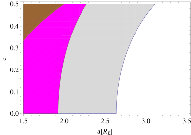
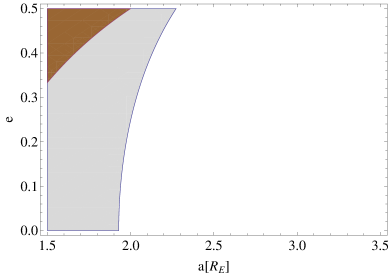
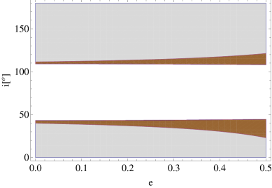
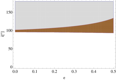
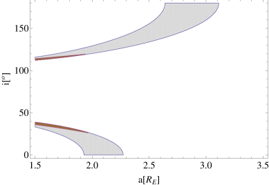
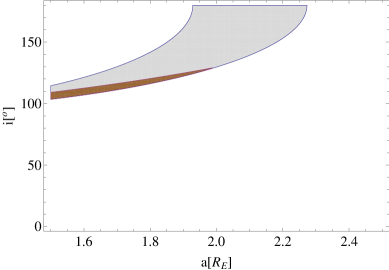
Figure 4. The regions in the $(a,e)$ plane (top panels), $(e,i)$ plane (middle panels), $(a,i)$ plane (bottom panels), where equation (5.1) admits solutions. Semi-secular resonances with $\alpha=2$, $\beta=2$, $\gamma=2$ (left column) $\alpha=0$, $\beta=2$, $\gamma=2$ (right column). Legend: white – no solutions, light grey – one solution, purple – two solutions, brown–colliding orbits.

As an example, let us consider the resonances with $\alpha=0$, $\beta=\gamma=2$ and $\alpha=\beta=\gamma=2$, respectively. Then, analyzing the conditions stated in Proposition 10, we compute the regions in the $(a,e)$ plane which admit solutions (see Figure 4).

In a similar way to Proposition 10, one can prove the following result.

Proposition 11.

Within the quadrupolar approximation (3.1), for given values of $e$ and $i$ the resonance relation (5.1) with fixed $\alpha$, $\beta$, $\gamma$ admits solutions for

$$a=R_{E}({A\over\gamma})^{2\over 7}$$

with

$$A=4.98\alpha(1-e^{2})^{-2}(5\cos^{2}i-1)-9.97\beta(1-e^{2})^{-2}\cos i\ ,$$

provided

$$4.98\alpha(1-e^{2})^{-2}(5\cos^{2}i-1)-9.97\beta(1-e^{2})^{-2}\cos i>\gamma\ .$$

For the same resonances, that is $\alpha=0$, $\beta=\gamma=2$ and respectively $\alpha=\beta=\gamma=2$ we compute in Figure 4 the regions in the $(e,i)$ plane where equation (5.1) admits solutions.

Finally, we have the following result.

Proposition 12.

Within the quadrupolar approximation (3.1), for given values of $a$ and $i$ the resonance relation (5.1) with given $\alpha$, $\beta$, $\gamma$ admits solutions for

$$e=\sqrt{1-\sqrt{A\over\gamma}}$$

with

$$A=(4.98\alpha(5\cos^{2}i-1)-9.97\beta\cos i)({R_{E}\over a})^{7\over 2}\ ,$$

provided

$$(4.98\alpha(5\cos^{2}i-1)-9.97\beta\cos i)\ ({R_{E}\over a})^{7\over 2}<\gamma\ .$$

For the same semi–secular resonances as above, Figure 4 shows the regions in the $(a,i)$ plane where the equation (5.1) admits solutions.

Summarizing the results obtained by applying Propositions 10, 11, 12, we may conclude that for the resonance with $\alpha=\beta=\gamma=2$ the equation (5.1) might have 0, 1 or 2 solutions, depending on the values of $a$, $e$ and $i$; for instance, fixing the eccentricity, let say $e=0.3$, then, we find that for $a>2.8R_{E}$ there are no solutions, for $a\in[2.044R_{E},2.798R_{E}]$ there is one solution, while for $a<2.044R_{E}$ one finds two solutions (see Figure 4). On the contrary, for the resonance with $\alpha=0$, $\beta=\gamma=2$, the case $(iii)_{b}$ of Proposition 10 cannot be fulfilled, that is one might find at most one solution.

The location of the resonances with $\alpha=\beta=\gamma=2$ and $\alpha=0$, $\beta=\gamma=2$, respectively, is analyzed numerically in Figure 5, which complements the results given in Figure 4. Grey shaded regions define the zone in which (5.1) can be solved, collisional regimes are highlighted in brown. Figure 5 numerically validates the Propositions 10, 11, 12 (compare with Figure 4 where the results are obtained by simply representing the regions described by these Propositions). In Figure 5, contours are shown for different values of orbital parameters as shown in the plot legends.

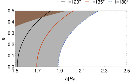
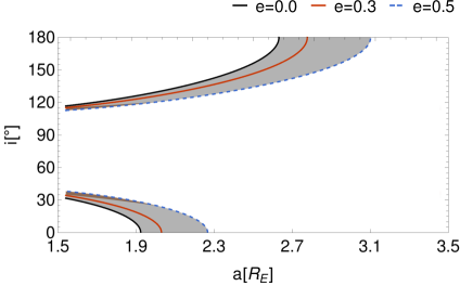
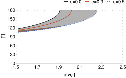
Figure 5. Location of semi-secular resonances in $(a,e)$-space (top) and $(a,i)$-space (bottom) for the $\alpha=2$, $\beta=2$, $\gamma=2$ (left) and the $\alpha=0$, $\beta=2$, $\gamma=2$ resonance (right). The full solution space is shown in grey, brown regions define parameters that lead to collision with Earth.

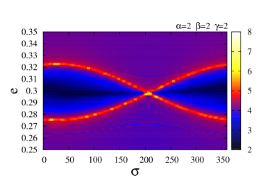
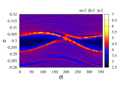
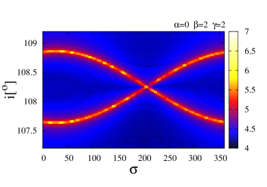
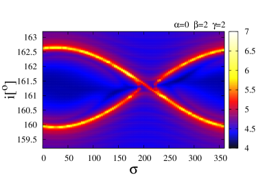
Figure 6. Top panels: FLI for the evection resonance with $\alpha=\beta=\gamma=2$ as a function of the resonant angle $\sigma=2\omega+2\Omega-2M_{S}$. The results are obtained for: $a=1.91R_{E}$, $i=19.04^{o}$, $\Omega=0^{o}$ and the value of $M_{S}$ at the epoch J2000, that is $M_{S}=357.5256^{o}$ (left panel), and respectively $a=2.3R_{E}$, $i=135.95^{o}$, $\Omega=0^{o}$ and $M_{S}=357.5256^{o}$ (right panel). Bottom panels: FLI for the resonance with $\alpha=0$, $\beta=\gamma=2$ as a function of the resonant angle $\sigma=2\Omega-2M_{S}$. The results are obtained for: $a=1.392R_{E}$, $e=0.05$, $\omega=0^{o}$ and the value of $M_{S}$ at the epoch J2000, that is $M_{S}=357.5256^{o}$ (left panel), and respectively $a=1.91R_{E}$, $e=0.05$, $\omega=0^{o}$ and $M_{S}=357.5256^{o}$ (right panel).

The predicted position of the semi-secular resonances is confirmed by a cartographic study based on the computation of the FLIs. For instance, by solving the equation (5.1) for $\alpha=\beta=\gamma=2$, we find the solutions $i=19.04^{o}$ and $i=123.04^{o}$ for $e=0.3$ and $a=1.91R_{E}$, and respectively the unique solution $i=135,95^{o}$ for $e=0.3$ and $a=2.3R_{E}$. Figure 6 shows the FLI values for $i=19.04^{o}$ and $a=1.91R_{E}$ (left panel) and respectively $i=135.95^{o}$ and $a=2.3R_{E}$ (right panel). For these parameters, pendulum–like plots are obtained; the separatrix divides the phase space into regions where the resonant angle $\sigma=2\omega+2\Omega-2M_{S}$ librates or circulates. As far as the resonance $\alpha=0$, $\beta=\gamma=2$, is considered, we compute the FLIs as in Figure 6 and we infer a similar dynamical behavior as for $\alpha=\beta=\gamma=2$ in the sense that the phase–space is still similar to a pendulum. However, the resonances with $\alpha=0$ lead to variations of the inclination, while the eccentricity remains constant as it is shown in Section 5.2. In fact, a more detailed study of the dynamics of Solar semi-secular resonances is provided in Section 5.2, where both types of commensurabilities, with $\alpha=0$ and $\alpha\neq 0$, are analyzed for small as well as moderate values of the eccentricity.

5.2. Around the Solar semi-secular resonance

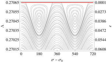
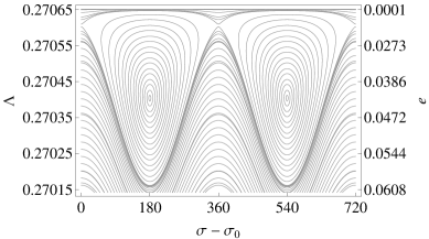
Figure 7. Phase portrait of the resonance in the ($\sigma-\sigma_{0},\Lambda$)-plane, showing a bifurcation of equilibria for the resonance with $\alpha=\beta=\gamma=2$: stable equilibrium points at $\sigma-\sigma_{0}=180^{o}+360^{o}k$, $k\in\mathbb{Z}$ (left plots), and respectively stable and unstable equilibria at $\sigma-\sigma_{0}=180^{o}k$, $k\in\mathbb{Z}$ (right plot). The plots are obtained for some fixed values of $L$ and $\Gamma$, computed via (2.1) and (5.6) by giving $a$, $e$ and $i$. For the left plot $L$ and $\Gamma$ correspond to $a=1.937R_{E}$, $e=0.1$, $i=1.51^{o}$, while the right plot is obtained for $a=1.937R_{E}$, $e=0.1$, $i=2.01^{o}$. The values of $\Lambda$ are expressed with respect to the following units of length and time: the geostationary distance is unity (it amounts to 42 164.1696 km) and the period of Earth’s rotation is equal to $2\pi$. On the left plot, all points on the horizontal line $e=0$ (red line) are equilibrium points, that is the conditions of the case $(a)_{1}$ are satisfied. On the right part we provide the value of the eccentricity computed via the relation $2\Lambda=L\sqrt{1-e^{2}}$.

In this Section we introduce a model that describes the dynamics in a neighborhood of a Solar semi-secular resonance of the form

$$\alpha\dot{\omega}+\beta\dot{\Omega}-\gamma\dot{M}_{S}=0$$ (5.5)

for $\alpha,\beta\in\mathbb{Z}$, $\gamma\in\mathbb{Z}\backslash\{0\}$. Since for small and moderate eccentricities, that is $e\leq 0.5$, the semi–secular resonances occur in LEO and in vicinity of the LEO region (see Figures 4–5), from (LABEL:MomeagaOmega_var) it follows that $\omega$ and $\Omega$, as well as $M_{S}$, $M_{M}$ and $M$ are fast angles in comparison with the resonant angle $\sigma=\alpha\omega+\beta\Omega-\gamma M_{S}$. Considering a specific semi-secular resonance, its dynamics can be described by a reduced model, which is obtained by averaging the full Hamiltonian over $M$, $M_{S}$, $M_{M}$, $\omega$ and $\Omega$, and retaining only the secular and resonant terms. Thus, we deduce that the reduced Hamiltonian has the form:

$$\mathcal{H}_{\alpha\beta\gamma}(G,H,\Phi,\omega,\Omega,M_{S};L)=h_{0}(G,H;L)+h_{1}(G,H;L)\cos(\alpha\omega+\beta\Omega-\gamma M_{S}-\sigma_{0})+\dot{M}_{S}\Phi\,,$$

where the dummy action $\Phi$, conjugated to $M_{S}$, was introduced to make $\mathcal{H}_{\alpha\beta\gamma}$ autonomous, $\sigma_{0}$ is a constant, $L$ is also a constant, while $h_{0}$ and $h_{1}$ are known functions.

As noticed in Figure 6, from a dynamical perspective the semi-secular resonances can be grouped in two classes: resonances with $\alpha\neq 0$ and resonances with $\alpha=0$, respectively. Let us consider first the resonances with $\alpha\neq 0$. We introduce the canonical change of coordinates $(G,H,\Phi,\omega,\Omega,M_{S})\longrightarrow(\Lambda,\Gamma,Z,\sigma,\Omega,M_{S})$, where

$$\Lambda=\frac{1}{\alpha}G\,,\qquad\Gamma=H-\frac{\beta}{\alpha}G\,,\qquad Z=\Phi+\frac{\gamma}{\alpha}G\,.$$ (5.6)

Clearly, $\Omega$ and $M_{S}$ are ignorable variables in the new Hamiltonian, so $\Gamma$ and $Z$ are constants of motion. After neglecting constant terms, we obtain the one degree-of-freedom Hamiltonian:

$$\mathcal{K}_{\alpha\beta\gamma}(\Lambda,\sigma;\Gamma,L)=f_{0}(\Lambda;\Gamma,L)-\gamma\dot{M}_{S}\Lambda+f_{1}(\Lambda;\Gamma,L)\cos(\sigma-\sigma_{0})\,,$$

where $f_{0}(\Lambda;\Gamma,L)=h_{0}(\alpha\Lambda,\Gamma+\beta\Lambda;L)$ and $f_{1}(\Lambda;\Gamma,L)=h_{1}(\alpha\Lambda,\Gamma+\beta\Lambda;L)$.

The equilibria are obtained by solving the equations

$$\frac{\partial f_{0}}{\partial\Lambda}-\gamma\dot{M}_{S}+\frac{\partial f_{1}}{\partial\Lambda}\cos(\sigma-\sigma_{0})=0,\qquad f_{1}\sin(\sigma-\sigma_{0})=0\,.$$ (5.7)

A closer look on the Solar disturbing function (2.24) reveals the fact that for all semi-secular resonances of this class the function $f_{1}$ is of second order in the eccentricity. Then, an analysis of the equations (5.7) shows that we can distinguish the following cases.

Case $(a)$: if there exist $L_{0}$ and $\Gamma_{0}$ so that $f_{1}(\Lambda;\Gamma_{0},L_{0})=0$ admits solutions, let $\Lambda_{0}$ be one of them (for instance, for the resonance with $\alpha=\beta=\gamma=2$ the function $f_{1}$ vanishes either for $e=0$ or $i=180^{0}$). In addition, one has either $(a)_{1}:$ $\frac{\partial f_{1}}{\partial\Lambda}(\Lambda_{0};\Gamma_{0},L_{0})=0$ and $\frac{\partial f_{0}}{\partial\Lambda}(\Lambda_{0};\Gamma_{0},L_{0})-\gamma\dot{M}_{S}=0$ or $(a)_{2}:$ $\frac{\partial f_{1}}{\partial\Lambda}(\Lambda_{0};\Gamma_{0},L_{0})\neq 0$ and $\Bigl{|}\frac{\partial f_{0}}{\partial\Lambda}(\Lambda_{0};\Gamma_{0},L_{0})-\gamma\dot{M}_{S}\Bigr{|}\leq\Bigl{|}\frac{\partial f_{1}}{\partial\Lambda}(\Lambda_{0};\Gamma_{0},L_{0})\Bigr{|}$, then the canonical equations admit some equilibrium points that are not similar to the pendulum-like equilibria. Indeed, in the case $(a)_{1}$ all points of the form $(\Lambda_{0},\sigma)$ with $\sigma\in\mathbb{R}$ are equilibrium points; we are dealing with a more complex problem than the pendulum (compare with [Henrard & Lemaître (1983)]). These points define a line in the $(\Lambda,\sigma)$ plane. On the other hand, the condition of the case $(a)_{2}$ assures that in the domain $\sigma\in[0^{o},360^{o})$ there exists at least one value $\sigma_{1}$, or at most two values $\sigma_{1}$ and $\sigma_{2}$, such that $(\Lambda_{0},\sigma_{1})$, respectively $(\Lambda_{0},\sigma_{1})$ and $(\Lambda_{0},\sigma_{2})$, are equilibrium points.

Case $(b)$: if $\sigma=\sigma_{0}+180^{o}k$, where $k\in\mathbb{Z}$, then the second equation of (5.7) is identically satisfied. Substituting $\sigma$ in the first equation of (5.7) we deduce the values of $\Lambda$ corresponding to equilibria, provided they exist. In this case, we can obtain either both stable and unstable equilibrium points as in the case of a pendulum, let us label this case by $(b)_{1}$, or just stable equilibria, denoted hereafter by $(b)_{2}$. Indeed, after substituting $\sigma=\sigma_{0}+180^{o}k$ in the first equation of (5.7), we find that for some values of $L$ and $\Gamma$ this equation has solutions for any $k\in\mathbb{Z}$; in some cases the first equation of (5.7) can be solved only when $k$ has the form $k=2k_{1}+1$ with $k_{1}\in\mathbb{Z}$.

These aspects are depicted in Figures 6 and 7 which address the semi-secular resonance with $\alpha=\beta=\gamma=2$. More precisely, for large enough eccentricities the phase space is similar to a pendulum as it is shown in Figure 6. However, for small eccentricities we may have different types of equilibria and Figure 7 exemplifies the cases described above. Figure 7 shows the phase portrait of the resonance. On the left all points on the horizontal line $e=0$ (red line) are equilibrium points, that is the conditions of the case $(a)_{1}$ are satisfied. Indeed, since $f_{1}=O(e^{2})$, one has $f_{1}|_{e=0}=0$, $\frac{\partial f_{1}}{\partial e}|_{e=0}=0$ and from $\frac{\partial f_{1}}{\partial\Lambda}=\frac{\partial f_{1}}{\partial e}\frac{\partial e}{\partial\Lambda}$ we deduce $\frac{\partial f_{1}}{\partial\Lambda}\mid_{e=0}=0$. Moreover, the left plot of Figure 7 illustrates that the conditions of the case $(b)_{2}$ are satisfied, thus providing stable equilibria at $\sigma=\sigma_{0}+180^{o}k$ and $e=0.0359$ (or equivalently $\Lambda=0.270476$), but there do not exist hyperbolic points similar to those of a pendulum.

The left panel of Figure 7 is obtained for some fixed values of $L$ and $\Gamma$, computed via (2.1) and (5.6) by taking $a=1.937R_{E}$, $e=0.1$ and $i=1.51^{o}$. A small change of the parameters $L$ and $\Gamma$ can lead to a bifurcation of equilibria. Indeed, by considering a slightly different value of $\Gamma$, which corresponds to $a=1.937R_{E}$, $e=0.1$ and $i=2.01^{o}$, we obtain a different phase portrait as it is illustrated by the right panel of Figure 7. The conditions of the case $(a)$ are not satisfied. However, the conditions of the case $(b)_{1}$ hold true; the phase space is topologically equivalent to a pendulum, but the stable and unstable equilibria are located at different values of $\Lambda$.

Let us consider now the class of resonances with $\alpha=0$. Clearly, it is necessary that $\beta\neq 0$ since otherwise the resonance condition (5.5) cannot be fulfilled. We proceed as above and we consider the canonical change of coordinates $(G,H,\Phi,\omega,\Omega,M_{S})\longrightarrow(G,S,Y,\omega,\sigma,M_{S})$, where

$$S=\frac{1}{\beta}H\,,\qquad\qquad Y=\Phi+\frac{\gamma}{\alpha}H\,.$$

Clearly, $\omega$ and $M_{S}$ are ignorable variables in the new Hamiltonian, so $G$ and $Y$ are constants of motion. Implementing the transformation and neglecting constant terms, we obtain the one degree-of-freedom Hamiltonian:

$$\mathcal{K}_{0\beta\gamma}(S,\sigma;G,L)=g_{0}(S;G,L)-\gamma\dot{M}_{S}S+g_{1}(S;G,L)\cos(\sigma-\sigma_{0})\,,$$

where $g_{0}(S;G,L)=h_{0}(G,\beta S;L)$ and $g_{1}(S;G,L)=h_{1}(G,\beta S;L)$.

The equilibria are obtained by solving the equations

$$\frac{\partial g_{0}}{\partial S}-\gamma\dot{M}_{S}+\frac{\partial g_{1}}{\partial S}\cos(\sigma-\sigma_{0})=0,\qquad g_{1}\sin(\sigma-\sigma_{0})=0\,.$$

The analysis of the equilibria can be made similarly to the study performed for the other group of Solar semi–secular resonances. A key point of the discussion is related to the equation $g_{1}(S;G,L)=0$. We underline that there is a difference with respect to the other group of semi-secular resonances, since the equation $f_{1}(\Lambda;\Gamma,L)=0$ always has solutions, while the equation $g_{1}(S;G,L)=0$ can have no solutions. Let us consider the resonance with $\alpha=0$, $\beta=2$, $\gamma=2$. From (2.24) we deduce that the function $g_{1}$, expressed in terms of the orbital elements, has the form $g_{1}=c\,a^{2}(1+\frac{3}{2}e^{2})\sin^{2}i$, where $c$ is a constant. From Propositions 11 and 12 (see also the left plots of Figure 4), this resonance occurs for $i\geq 90^{o}$; as a consequence, equation $g_{1}(S;G,L)=0$ cannot be satisfied, unless $i=180^{o}$ and we conclude that this resonance is topologically equivalent to a pendulum as long as $i<180^{o}$ (see Figure 6, bottom panels). This might not be the case for other resonances and each of them should be studied individually.

5.3. Lunar semi-secular resonances

Lunar semi-secular resonances are characterized by a relation of the form

$$\alpha\dot{\omega}+\beta\dot{\Omega}+\alpha_{M}\dot{\omega}_{M}+\beta_{M}\dot{\Omega}_{M}-\gamma\dot{M}_{M}=0\ ,$$ (5.8)

where, in the quadrupolar approximations for the Lunar and Solar expansions, we consider $\alpha,\alpha_{M}=0,\pm 2$, $\beta,\beta_{M}=0,\pm 1,\pm 2$, $\gamma\not=0$. We can set $\dot{M}_{M}=13.06$ deg/day, $\dot{\omega}_{M}=0.164$ deg/day, $\dot{\Omega}_{M}=-0.053$ deg/day. Hence, the resonance (5.8) becomes:

$$4.98\alpha({R_{E}\over a})^{7\over 2}(1-e^{2})^{-2}(5\cos^{2}i-1)-9.97\beta({R_{E}\over a})^{7\over 2}(1-e^{2})^{-2}\cos i$$ (5.9)

$$+ (0.164\alpha_{M}-0.053\beta_{M}-13.06\gamma)=0\ .$$

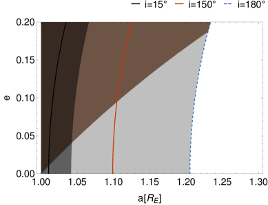
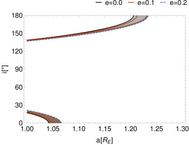
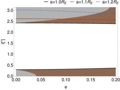
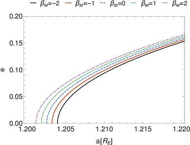
Figure 8. Location of Lunar semi-secular resonances with $\alpha=2$, $\beta=1$, $\alpha_{M}=2$, $\beta_{M}=2$, $\gamma=2$ (top-left, top-right, bottom-left) and $\alpha_{M}=0$, $\beta_{M}=-2,\dots,2$ (bottom-right). The full solution space is shown in grey, brown regions define parameters that lead to collision with Earth. Upper left, dark: 2 solutions, light: 1 solution.

The possible solutions for $\alpha=2$, $\beta=1$, $\gamma=2$, $\alpha_{M}=2$, $\beta_{M}=2$ and $\alpha_{M}=0$, $|\beta_{M}|\leq 2$ are shown in Figure 8. In the upper left panel we show the $(a,e)$ plane for the case with $\alpha_{M}=2$, where (5.8) admits one solution (dark grey), two solutions (grey), and no solution (white), where the regions have been obtained using Proposition 13 (see just below). In the brown region the orbiting object collides with the Earth at perigee. Three contours are shown for fixed values of inclination in black, red, and dashed-blue respectively. In the upper-right and lower-left panel we show the possible solutions of (5.8) for the same case ($\alpha_{M}=2$) in the $(a,i)$ and $(e,i)$ plane, respectively. Here, grey marks regions, where solutions can be found, solutions with one fixed orbital parameter (see legends at the top) are shown in color code. To demonstrate the effect of varying $\beta_{M}$ on the contours, we plot a magnification of the $(a,e)$ plane of the previous case, but with $\alpha_{M}=0$ and $\beta_{M}=-2,\dots,2$ in the bottom-right panel of Figure 8. A slight shift of the contours with increasing $\beta_{M}$ to smaller values of the semi-major axis $a$ is clearly visible. As it can be inferred from Figure 8, Lunar semi-secular resonances are very close to the Earth. Therefore, from a practical perspective these resonances are less relevant for the Earth-Moon system; resonant orbits are either colliding orbits or escape orbits, as effect of the atmospheric drag.

Proposition 13.

Within the quadrupolar approximation (3.1), consider the resonance relation (5.9) with given $\alpha$, $\beta$, $\alpha_{M}$, $\beta_{M}$, $\gamma$. For given values of $a$, $e$, let us introduce the quantities

$$A=4.98({R_{E}\over a})^{7\over 2}(1-e^{2})^{-2}\ ,$$

and let $\Gamma$ be defined as

$$\Gamma=-0.164\alpha_{M}+0.053\beta_{M}+13.06\gamma\ .$$

Then, the conclusions of Proposition 10 hold with $\gamma$ replaced by $\Gamma$ (which depends on the free parameters $\alpha_{M}$, $\beta_{M}$, $\gamma$). Hence, for $\Delta_{L}$ defined as

$$\Delta_{L}=\beta^{2}A^{2}+5\alpha(\alpha A+\Gamma)A\ ,$$

let us consider the following inequalities:

$$\beta^{2}A^{2}+5\alpha(\alpha A+\Gamma)A\geq 0$$ (5.10)

$$-(5\alpha+\beta)A\leq\sqrt{\Delta_{L}}\leq(5\alpha-\beta)A$$ (5.11)

$$-(5\alpha-\beta)A\leq\sqrt{\Delta_{L}}\leq(5\alpha+\beta)A.$$ (5.12)

Then, we have the following cases: $(i)$ if $\Delta_{L}<0$ or $|{{\beta A\pm\sqrt{\Delta_{L}}}\over{5\alpha A}}|>1$, then (5.9) admits no solutions; $(ii)$ if (5.10) and just one of the conditions (5.11) and (5.12) are satisfied, then (5.9) admits one solution; $(iii)$ if (5.10), (5.11), (5.12) are satisfied, then (5.9) admits two solutions.

In a similar way, one can prove the following result.

Proposition 14.

Within the quadrupolar approximation (3.1), the resonance relation (5.9) with given $\alpha$, $\beta$, $\gamma$ admits solutions for

$$a=R_{E}({A\over\Gamma})^{2\over 7}$$

with

$$A=4.98\alpha(1-e^{2})^{-2}(5\cos^{2}i-1)-9.97\beta(1-e^{2})^{-2}\cos i\ ,\qquad\Gamma=-0.164\alpha_{M}+0.053\beta_{M}+13.06\gamma\ ,$$

provided

$$4.98\alpha(1-e^{2})^{-2}(5\cos^{2}i-1)-9.97\beta(1-e^{2})^{-2}\cos i>\Gamma\ .$$

We conclude this section with the following Proposition.

Proposition 15.

Within the quadrupolar approximation (3.1), the resonance relation (5.9) with given $\alpha$, $\beta$, $\gamma$ admits solutions for

$$e=\sqrt{1-{\sqrt{A\over\Gamma}}}$$

with

$$A=(4.98\alpha(5\cos^{2}i-1)-9.97\beta\cos i)({R_{E}\over a})^{7\over 2}\ ,\qquad\Gamma=-0.164\alpha_{M}+0.053\beta_{M}+13.06\gamma\ ,$$

provided

$$(4.98\alpha(5\cos^{2}i-1)-9.97\beta\cos i)\ ({R_{E}\over a})^{7\over 2}<\Gamma\ .$$

6. A characterization of secular resonances

Secular resonances depend on the rates of variation of slowly varying quantities, typically the argument of perigee and the longitude of the ascending node. We distinguish again between Solar and Lunar resonances which are, respectively, described in Sections 6.1 and 6.2. In Section 6.1 we obtain that the commensurability relation describing the Solar secular resonances turns out to be a condition on the inclination in terms of the coefficients entering the resonance relation. In Section 6.2 we discuss the Lunar secular resonances, which can be treated as in Propositions 13, 14, 15 describing the Lunar semi-secular resonances.

6.1. Solar secular resonances

Given that the Solar rates of variation of the argument of perigee and the longitude of the ascending node are zero, the Solar secular resonances occur whenever

$$\alpha\dot{\omega}+\beta\dot{\Omega}=0$$ (6.1)

for some $\alpha$, $\beta\in\mathbb{Z}$. It might look strange to refer to (6.1) as Solar secular resonances, since the elements of the Sun do not occur at all in this expression, due to the fact that we have set to zero both $\dot{\omega}_{S}$ and $\dot{\Omega}_{S}$. However, we will keep this terminology for consistency with the previous and following sections.

The relation (6.1) can be written as

$$({R_{E}\over a})^{7\over 2}(1-e^{2})^{-2}\ [4.98\alpha(5\cos^{2}i-1)-9.97\beta\cos i]=0\ .$$

The above expression depends just on the inclination and it is satisfied whenever we have

$$\cos i={{9.97\beta\pm\sqrt{99.4009\beta^{2}+496.506\alpha^{2}}}\over{49.8\alpha}}\ .$$

Since $99.4009\beta^{2}+496.506\alpha^{2}\geq 0$, we have two real solutions, which have a physical meaning provided that $|\cos i|\leq 1$, which gives a condition on $\alpha$, $\beta$ to have Solar secular resonances.

For a detailed investigation of Solar secular resonances depending just on the inclination, we refer the reader to [Celletti et al. (2016a)] and [Hughes (1980)]. Here, it is worthwhile to mention that the resonances (6.1) include the cases $\dot{\omega}=0$, corresponding to the critical inclinations ($i=63.4^{o}$, $i=116.4^{o}$), and $\dot{\Omega}=0$, corresponding to polar orbits.

6.2. Lunar secular resonances

The Lunar secular resonances occur whenever

$$\alpha\dot{\omega}+\beta\dot{\Omega}+0.164\alpha_{M}-0.053\beta_{M}=0$$

for some $\alpha$, $\beta,\alpha_{M},\beta_{M}\in\mathbb{Z}$; this relation can be written as

$$({R_{E}\over a})^{7\over 2}(1-e^{2})^{-2}\ [4.98\alpha(5\cos^{2}i-1)-9.97\beta\cos i]=0.053\beta_{M}-0.164\alpha_{M}\ .$$

The same result of Proposition 13 holds with $\gamma=0$ to find the inclination, having fixed $a$, $e$, Proposition 14 with $\gamma=0$ to determine the semimajor axis, having fixed $e$, $i$, Proposition 15 with $\gamma=0$ to find the eccentricity, having fixed $a$, $i$.

An example of the location of the Lunar secular resonances is given in Figure 9 as a function of the orbital elements $a$, $e$, $i$. In the example we choose $\alpha=2$, $\beta=1$, $\alpha_{M}=0$ and $\beta_{M}=\pm 1$. In the upper plots dark grey marks regions where two distinct solutions of above equations are possible (in the sense of Proposition 13). For our parameters and the case $\beta_{M}=-1$ this region can be found in the space $(a,e)$ for values up to $a\simeq 4.5-5.0R_{E}$. For the case $\beta=1$ this region of two distinct solutions is increased up to values $a\simeq 6.0-7.0R_{E}$. Moreover, an additional region in the space $(a,e)$ is present, starting from $a\simeq 6.0$ where only one solution to the condition for Lunar secular resonances exists (shown in light grey in the upper right plot of Figure 9). The reason for the different topologies in the solution space becomes clear when looking at the regions of possible solutions in the space $(a,i)$ (shown at the bottom of Figure 9). Two symmetric solutions exist for the case $\beta=-1$ up to a certain value in $a$, while in case of $\beta=1$ the two distinct solution branches are asymmetric. At the moment, when the lower branch stops at some value in $a$ (that depends on the specific value chosen for eccentricity $e$) the upper branch still extends farther to larger values in $a$, which yields the region in solution space with one solution, according to Proposition 13.

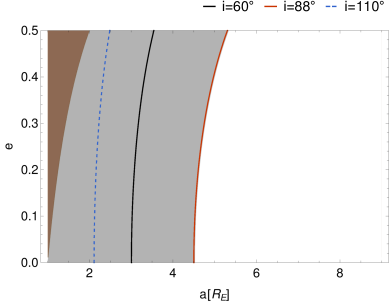
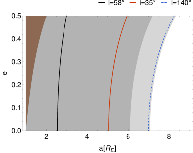
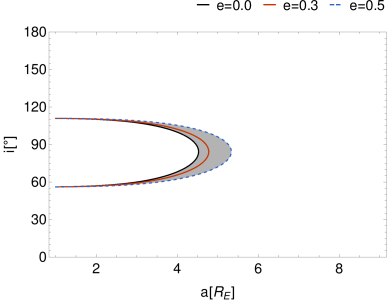
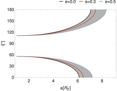
Figure 9. Location of Lunar secular resonances in $(a,e)$-space (top) and $(a,i)$-space (bottom) for $\alpha=2$, $\beta=1$, $\alpha_{M}=0$, and $\beta_{M}=-1$ (left) and respectively $\beta_{M}=+1$ (right). In the top panel, dark grey marks regions with two solutions, light grey marks regions with one solution. At the bottom panel, grey defines the space where solutions can be found. Contours are shown for specific parameters provided in the plot legends. Parameters that lead to collisions are highlighted in brown.

We remark that another class of resonances is given by the mean motion resonances between the orbital period of the object and the Moon, which correspond to solutions of the equation $\alpha\dot{M}+\beta\dot{M}_{M}=0$ for suitable $\alpha,\beta\in\mathbb{Z}$; however, here we will not be interested to such resonances, since they typically occur far from the Earth, well outside the geostationary orbit.

7. Conclusions

Despite the fact that several decades have lapsed since the first satellite was launched in space, the dynamics of an object moving around the Earth is still an intriguing subject, especially when considering the large number of space debris populating our sky. Within such context, it is remarkable that the problem presents different time scales, since the Hamiltonian function describing the dynamics depends on short-period angles (the mean anomaly of the object and the sidereal time), secular angles (the arguments of perigee and the longitudes of the ascending node of the object, Sun and Moon), semi-secular angles given by the mean anomalies of Moon and Sun (which have, respectively, a period of one month and one year). This remark motivates the study of different types of resonances, according to the quantities which are involved in the commensurability relation defining the resonance. Based on elementary computations, our aim is to characterize in the quadrupolar approximation the different resonances according to the values of the orbital elements, namely semimajor axis, eccentricity and inclination. This allows us to specify the orbital elements regions where the resonances can be found. We summarize below our main results.

In Section 4 we study tesseral resonances of order $j:\ell$:

• for fixed values of $a$, $e$, we obtain an expression for the inclination (Proposition 7);

• for fixed values of $e$, $i$, we obtain an equation for the semimajor axis (Proposition 8);

• for fixed values of $a$, $i$, we get an equation for the eccentricity (Proposition 9).

In Section 5.1 we study the Solar semi-secular resonances and we obtain the following results:

• for given values of $a$, $e$, we obtain an equation for $\cos i$, whose discussion leads to obtain bounds on the elements, ensuring the existence of zero, one, two solutions (Proposition 10);

• for given values of $e$, $i$, we obtain a value for the semimajor axis and bounds on $e$, $i$, ensuring the existence of solutions (Proposition 11);

• for given values of $a$, $i$, we obtain an expression for the eccentricity and bounds on $a$, $i$, ensuring the existence of solutions (Proposition 12).

Similar results are obtained in Section 5.3 for the Lunar semi-secular resonances as provided by Propositions 13, 14, 15.

Finally, in Section 6 we shortly analyze the Solar (Section 6.1) and Lunar (Section 6.2) secular resonances, which are extensively treated in [Celletti et al. (2016a)] and [Hughes (1980)].

Appendix: The Fast Lyapunov Indicator (FLI)

FLI is a familiar chaos tool used to numerically investigate the stability of a dynamical system. Comparing the values of the FLIs as the initial conditions or parameters are varied, one can distinguish between regular, resonant or chaotic motions (see [Froeschlé et al. (1997)], [Guzzo & Lega (2018)]). Here we briefly recall the definition of FLI and we describe how it is computed for our particular system.

The Lyapunov Characteristic Exponent (see [Benettin et al. (1980)]) provides evidence of the chaotic character of the dynamics of a given dynamical system, since it measures the divergence of nearby trajectories. For a phase space of dimension $N$, there exist $N$ Lyapunov exponents, although the largest one is the most significative and is what we refer to as the Lyapunov exponent. This choice is motivated by the exponential rate of divergence, since the greatest exponent dominates the overall separation.

Lyapunov exponents can be computed as follows ([Arnold et al. (1986)]): let ${\underline{\xi}}=(L,G,H,M,\omega,\Omega)$ be the phase state associated with the Hamiltonian, say $\mathcal{H}$ (see Section 2). We can generically denote the evolution in phase space as determined by the vector field

$$\dot{\underline{\xi}}={\underline{f}}({\underline{\xi}})\ ,\qquad{\underline{\xi}}\in\mathbb{R}^{6}\ ,$$

and the evolution on the tangent space by the corresponding variational equations

$$\dot{\underline{\eta}}=\left({{\partial\underline{f}(\underline{\xi})}\over{\partial\underline{\xi}}}\right)\ {\underline{\eta}}\ ,\qquad{\underline{\eta}}\in\mathbb{R}^{6}\ .$$

We can assign the initial conditions by choosing $\underline{\xi}(0)$ and each component of $\underline{\eta}(0)={\eta}_{j}(0)\,\underline{{\hat{e}}}_{j}$ in a basis $\underline{{\hat{e}}}_{j}$ of the tangent space. Then, we can compute the quantities

$$\chi_{j}\equiv\lim_{t\to\infty}\lim_{||\underline{\eta}(0)||\to 0}{1\over t}\log{{|{\eta}_{j}(t)|}\over{|{\eta}_{j}(0)|}}\ ,\qquad j=1,...,6\ ,$$

where $\|\cdot\|$ denotes the Euclidean norm.

When dealing with a Hamiltonian dynamical system only $N/2$ of the $\chi_{j}$ are actually meaningful, so in our case we would have three exponents. In view of the exponential rate of divergence, we can concentrate on the greatest of them and estimate it by means of the formula

$$\chi\equiv\lim_{t\to\infty}{1\over{t}}\log{{||\underline{\eta}(t)||}\over{||\underline{\eta}(0)||}}\ ,$$

where $||\underline{\eta}(t)||$ is the phase-space Euclidean distance at time $t$ between trajectories at initial distance $||\underline{\eta}(0)||$.

In order to investigate the stability of the dynamics for the models described in the previous sections, we compute the so-called Fast Lyapunov Indicator, which is defined as the value of the largest Lyapunov characteristic exponent at a fixed time (see [Froeschlé et al. (1997)]). By comparing the values of the FLIs as initial conditions or parameters are varied, one obtains an indication of the dynamical character of the phase-space trajectories as well as of their chaoticity/regularity behaviour. The explicit computation of the FLI proceeds as follows: the FLI at a given time $T\geq 0$ is obtained by the expression

$${\rm FLI}(\underline{\xi}(0),\underline{\eta}(0),T)\equiv\sup_{0<t\leq T}\log||\underline{\eta}(t)||\ .$$

In practice, a reasonable choice of $T$ makes faster the computation of the FLI when compared with previous expressions for the $\chi$’s where, in principle, very long integration times are required to obtain a reliable convergence process. Analyzing the frequencies of the model, one can set the integration time $T$ as a good compromise between the accuracy of the computations and the length of the computer programs. For instance, the plots of Figure 3 are obtained by integrating, using a Runge-Kutta fourth order method, the canonical equations and the associated variational equations for an interval of 5 000 sidereal days. Such a value was calibrated against the frequency $\dot{M}$ of the fastest angle of the system (or equivalently the number of revolutions of the satellite around the Earth), and it is comparable with the number of revolutions that were taken in other papers, e.g. [Celletti & Galeş (2014), Celletti & Galeş (2015)].

References

- [Alessi et al. (2018)] E.M. Alessi, G. Schettino, A. Rossi, G.B. Valsecchi, Natural highways for end-of-life solutions in the LEO region, Celest. Mech. Dyn. Astron., 130, n.34, 2018.
- [Arnold et al. (1986)] L. Arnold, V. Wihstutz, Lyapunov exponents, a Survey, Lecture Notes in Mathematics 1186, 1-26, Springer, 1986.
- [Benettin et al. (1980)] G. Benettin, L. Galgani, A. Giorgilli, J.-M. Strelcyn, Lyapunov characteristic exponents for smooth dynamical systems and for Hamiltonian systems: A method for computing all of them, Meccanica 15, 9–30, 1980.
- [Celletti & Galeş (2014)] A. Celletti, C. Galeş, On the dynamics of space debris: 1:1 and 2:1 resonances, J. Nonlinear Science, 24, n. 6, 1231-1262, 2014.
- [Celletti & Galeş (2015)] A. Celletti, C. Galeş, Dynamical investigation of minor resonances for space debris, Celest. Mech. Dyn. Astr., 123, n. 2, 203–222, 2015.
- [Celletti et al. (2016a)] A. Celletti, C. Galeş, G. Pucacco, Bifurcation of lunisolar secular resonances for space debris orbits, SIAM J. Appl. Dyn. Syst., 15, 1352–1383, 2016.
- [Celletti & Galeş (2016b)] A. Celletti, C. Galeş, A study of the lunisolar secular resonance , Front. Astron. Space Sci. - Fundamental Astronomy, 31 March 2016 — http://dx.doi.org/10.3389/fspas.2016.00011
- [Celletti et al. (2017)] A. Celletti, C. Gales, G. Pucacco, A. Rosengren, Analytical development of the lunisolar disturbing function and the critical inclination secular resonance, Celest. Mech. Dyn. Astron., 127, n. 3, 259–283, 2017.
- [Celletti & Galeş (2018)] A. Celletti, C. Galeş, Dynamics of resonances and equilibria of Low Earth Objects, SIAM J. Appl. Dyn. Syst., 17, 203-235, 2018.
- [Ely & Howell (1997)] T.A. Ely, K.C. Howell, Dynamics of artificial satellite orbits with tesseral resonances including the effects of luni-solar perturbations, Dynamics and Stability of Systems, 12, n. 4, 243-269, 1997.
- [Froeschlé et al. (1997)] C. Froeschlé, E. Lega, R. Gonczi, Fast Lyapunov indicators. Application to asteroidal motion, Celest. Mech. Dyn. Astr., 67, n. 1, 41-62, 1997.
- [Gachet et al. (2017)] F. Gachet, A. Celletti, G. Pucacco, C. Efthymiopoulos, Geostationary secular dynamics revisited: application to high area-to-mass ratio objects, Celest. Mech. Dyn. Astr., 128, n. 2-3, 149-181, 2017.
- [Galeş(2012)] C. Galeş, A cartographic study of the phase space of the restricted three body problem. Application to the Sun-Jupiter-Asteroid system, Comm. Nonlinear Sc. Num. Sim., 17, 4721–4730, 2012.
- [Gkolias & Colombo (2019)] I. Gkolias, C. Colombo, Towards a sustainable exploitation of the geosynchronous orbital region, Celest. Mech. Dyn. Astr., 131, n. 19, 2019.
- [Guzzo & Lega (2018)] M. Guzzo, E. Lega, Geometric chaos indicators and computations of the spherical hypertube manifolds of the spatial circular restricted three-body problem, Physica D, 373, 35-58, 2018.
- [Henrard & Lemaître (1983)] J. Henrard, A. Lemaître, A second fundamental model for resonance, Celest. Mech., 30, n. 2, 197–218, 1983.
- [Hughes (1980)] S. Hughes, Earth satellite orbits with resonant lunisolar perturbations. I. Resonances dependent only on inclination, Proc. R. Soc. Lond. A, 372, 243–264, 1980.
- [Kaula (1962)] W.M. Kaula, Development of the lunar and solar disturbing functions for a close satellite, Astron. J., 67, 300-303, 1962.
- [Kaula (1966)] W.M. Kaula, Theory of Satellite Geodesy, Blaisdell Publ. Co., 1966.
- [Klinkrad (2006)] H. Klinkrad, Space Debris: Models and Risk Analysis, Springer-Praxis (Berlin-Heidelberg), 2006.
- [Lane (1989)] M. T. Lane, On analytic modeling of lunar perturbations of artificial satellites of the Earth, Celest. Mech. Dynam. Astr., 46, n. 4, 287-305, 1989.
- [Lhotka et al. (2016)] C. Lhotka, A. Celletti, C. Gales, Poynting-Robertson drag and solar wind in the space debris problem, Mon. Not. Roy. Ast. Soc., 460, 802-815, 2016.
- [Petit et al. (2018)] A. Petit, D. Casanova, M. Dumont, A. Lemaître, Dynamical lifetime survey of geostationary transfer orbits, Celest. Mech. Dyn. Astron. 130, n. 79, 2018.
- [Schettino et al. (2019)] G. Schettino, E.M. Alessi, A. Rossi, G.B. Valsecchi, A frequency portrait of Low Earth Orbits, Celest. Mech. Dyn. Astron. 131, n. 35, 2019.
- [Skoulidou et al. (2018)] D.K. Skoulidou, A.J. Rosengren, K. Tsiganis, G. Voyatzis, Dynamical lifetime survey of geostationary transfer orbits, Celest. Mech. Dyn. Astron. 130, n. 77, 2018.