Price impact of a trade is an important element in pre-trade and post-trade analyses. We introduce a framework to analyze the market price of liquidity risk, which allows us to derive an inhomogeneous Bernoulli ordinary differential equation. We obtain two closed form solutions, one of which reproduces the linear function of the order flow in Kyle (1985) for informed traders. However, when traders are not as asymmetrically informed, an S-shape function of the order flow is obtained. We perform an empirical intra-day analysis on Nikkei futures to quantify the price impact of order flow and compare our results with industry’s heuristic price impact functions. Our model of order flow yields a rich framework for not only to estimate the liquidity risk parameters, but also to provide a plausible cause of why volatility and correlation are stochastic in nature. Finally, we find that the market depth encapsulates the market price of liquidity risk.

1 Introduction

Whatever be the information content, it is no secret that transactions induce the market to move in the direction that reflects the price pressure over a time horizon. In Perold (1988), an institutional investor seeking to acquire or liquidate a substantial amount of a security is likely to cause the market price to deviate from the reference price, which is the market price prevailing at the time an investment decision has just been made. This deviation from the reference price—a component cost in the framework of Perold (1988)—is a reaction of the market to the institutional investor’s imminent need to trade.

Another cost of trading is known as the price impact cost or the market impact cost. It is the compensation the liquidity providers receive for rendering the service (of accommodation of mismatched order flow), and the market impact cost paid by liquidity demanders (Torre and Ferrari (1999)). According to Bouchaud (2010), the price impact is the result of the correlation between an incoming market order and the subsequent price change, in such a manner that the second buy trade is on average more expensive than the first because of its impact on the market price (and vice versa for sells). In other words, price impact is a post-trade explanation for the potential price disparity when a market order or marketable limit order is executed.

Given the risk of price uncertainty and disparity from the target price, what then is the market price of liquidity risk? More importantly, what is the price impact function that captures the price disparity or slippage? This paper attempts to provide some answers to these questions by introducing a risk-neutral measure that is consistent with the reality of no risk-free arbitrary opportunity. We then propose the market price of liquidity risk in a form similar to the market price of (market) risk. This idea forms the basis to obtain an analytical function for measuring the price impact. In other words, our analysis of the market price of liquidity risk leads us to the derivations of the price impact functions.

When the electronic market is open for trading, buy and sell orders are flowing into the exchange matching engine for execution. Aggregating over a trading period, the order flow (buyer-initiated trades less seller-initiated trades) provides an ex post measure of net demand for the asset, which translates into a market price. This relationship between the order flow and price is used by Evans and Lyons (2002) to show that order flow is a superior candidate for modeling the variation in foreign exchange rate compared to arguments along the lines of macroeconomics.

Even before trades occur, market participants are mindful that their market orders may potentially impact prices; traders will take into account the market impact of their trades. In other words, they know that there is going to be a disparity between the price $P_{t}$ at which their market order $X_{t}$ is executed and the price $S_{t}$ at which they wish their orders can be executed immediately. More often than not, $P_{t}$ is disadvantageous than $S_{t}$ to the traders. For that matter, price impact is created whenever $X_{t}\neq 0$ for all traders who consume liquidity. Moreover, Love and Payne (2008) show that for major currency pairs, using data sampled at the one-minute frequency, publicly announced macroeconomic information not only causes exchange rates to move, but also causes order flow to significantly change in a direction consistent with the exchange rate movement.

The interest in price impact and order flow spans several inter-related subjects of transaction costs, optimal trading strategies (Almgren and Chriss (2000) and Almgren (2012)), liquidity risk (Acharyaa and Pedersen (2005) and Amihud (2002)), price manipulation (Gatheral et al. (2012)). portfolio performance (Dai et al. (2016)), payoff replication (Liu and Yong (2005)), as well as dynamic hedging (Kennedy et al. (2009)). Obviously, there are voluminous papers on these subjects, and the list is by no means exhaustive. This paper adds to this rich literature by deriving from the market price of liquidity risk a functional form for the price impact as an analytical solution. Empirically, it is well known that when the size of order flow is small, the price impact is approximately linear. But when the trade size is very large, nonlinear effects become pronounced: concave when $X_{t}$ is positive and convex when $X_{t}$ is negative.

The formalism of this paper is similar to Çetin et al. (2004) and Huang and Ting (2008), among others, in that traded prices are dependent on the order size and another price referred to as the marginal price or the true price. The true price, in particular, originally appears in Roll (1984). In these papers, the true price is unobservable, as it is the price corresponding to the absence of trades, i.e., zero order flow. Furthermore, the literature of market microstructure is replete with the assumption that the true price is a geometric Brownian motion.

This paper further postulates that order flows are mean reverting. A standard transformation in stochastic calculus allows us to define the market price of liquidity. In making the true price process to be under the risk-neutral measure so as to reflect no risk-free arbitrage opportunity, we introduce the market price of (market) risk and also the market price of liquidity risk. We solve the Bernoulli differential equation and obtain a closed-form solution for the price impact function and the market price of liquidity risk. Both functions are dependent on the order flow. These results lead us to a natural measure of liquidity risk, much like volatility is a measure of market (price) risk. It turns out that the parameters of the market price of liquidity risk are encapsulated in a measure that can be interpreted as the market depth of the electronic market. The larger or deeper the market depth is, the market can be said to be more liquid.

Our model of price impact function is different from but complementary to the existing papers on price impact. For example, Wilinski et al. (2015) empirically find that price impact exhibits a sub-linear power-law scaling of daily-normalized volume. In Bouchaud et al. (2009), the theory of long-term resilience is put forth to model price impacts over different time lags. Gerig (2007) also develops a theory of price impact, with a focus on hidden order. He concludes that the impact of a hidden order is a concave function of its total volume, specifically, a logarithm function.

It is well beyond the scope of this paper to conduct an exhaustive review of closely related research. Nevertheless, the two above-mentioned theoretical works and other related papers converge to the general consensus that the price impact of a trade is a concave function of absolute volume normalized with certain heuristic schemes. By contrast, our price impact function is an S-shape function of order flow. Moreover, the other main difference is that our model is based on the market price of liquidity risk through the application of Itô’s calculus.

Price impact is a major concern for portfolio managers when they are about to reconstitute or re-balance their portfolios. Many prime broker-dealers have their own proprietary methods to measure the price impact. According to Ferraris (2008), price impact models used in the industry include the following:

1. BARRA model (Torre and Ferrari (1999))

   $$\alpha\sqrt{V}$$

2. Bloomberg’s model

   $$\frac{1}{2}\frac{\hbox{bid-ask spread}}{\hbox{price}}+\sqrt{\frac{\sigma^{2}/3}{250}}\sqrt{\frac{V}{0.3\times\hbox{EDV}}}$$

3. JP Morgan’s model

   $$95\%\times\frac{1.4}{\hbox{EPV}\times\sqrt{\hbox{EDV}}}\sigma^{2}V^{3/2}+5\%\times\frac{0.187}{\sqrt{\hbox{EDV}}}\sigma^{2}\sqrt{V}$$

In these phenomenological models, $\alpha$ is the parameter to be estimated, $\sigma$ is the volatility, and $V$ the volume. Respectively, EDV and EPV denote the expected daily volume and the expected period volume.

The first terms in the models of Bloomberg and JP Morgan correspond to the temporary price impact, and the second term is meant to estimate the permanent impact (see Ferraris (2008)). Temporary price impacts include the bid-ask spread. They affect prices temporarily by disturbing the supply and demand equilibrium. These transient disturbances are typically immediate at the point of transaction. On the other hand, permanent price impacts are caused by material information that will prompt investors to urgently update their belief about the value of the asset being traded. They have a relatively long lasting effect on the subsequent prices. Our price impact models capture mainly the temporary impact, and indirectly the permanent impact through the correlation with the order flows.

The industry models, while consistent with the insights gleaned from the market microstructure literature, are heuristic in nature. Generally, the price impact is assumed to be a square root of the trade size. For example, Hasbrouck (2004) uses the square root of volume to measure the price impact of futures traded in the CME pit. By contrast, our price impact function is derived from the framework of market price of liquidity risk through the application of stochastic calculus. It is based on the market reality of no risk-free arbitrage opportunity. Our model produces a linear price impact function of Kyle (1985) as a special case. In the more general case, we find that the price impact function is S-shape for all possible values of $X_{t}$. Empirically, we find that our model provides a better fit to the same data. Our price impact function may be a better model to estimate the potential price impact in pre-trade and post-trade analyses.

Furthermore, by adding a mean-reverting model of order flow $X_{t}$ to the geometric Brownian motion of the true price $S_{t}$, our modeling study shows that the randomness in $X_{t}$ causes the volatility of simple returns computed from trade prices to become stochastic. Likewise, the correlation between the simple return and the order flow has also become stochastic.

The paper will be presented as follows. Section 2 provides the basic assumptions that parallel those of Çetin et al. (2004). A key novel idea of our paper is to model the order flow dynamics as a mean-reverting process. Section 3 introduces two market prices of risks, leading to the inhomogeneous Bernoulli differential equation. In Section 4, we consider two special cases and derive the price impact functions in closed form. We provide empirical evidence in Section 5 that demonstrates that our S-shape price impact function is better than industry’s heuristic functions. Section 6 concludes.

2 Model Setup and Motivation

As defined by Lyons (2001), order flow is transaction volume that is signed. A trade at the ask price is said to be buyer-initiated (positive) and that at the bid price, seller-initiated (negative). Market orders and marketable limit orders are means by which transactions are initiated and executed. With immediacy, these trades consume liquidity provided by dealers and market makers. On electronic exchanges, liquidity is said to be provided by traders who submit limit orders, which are displayed on an electronic limit order book.

Order flow has many nuances; we define it for our model to avoid misunderstanding as follows. Over a specified time interval, say 1 minute, the order flow is computed by observed trades initiated by buyers and sellers. Specifically, the order flow $X_{t}$ is written as

$$X_{t}=X_{t}^{+}-X_{t}^{-},$$ (2.1)

where, over a time interval, $X_{t}^{+}$ is the aggregate volume of buyer-initiated trades and $X_{t}^{-}$ is the aggregate trade size of seller-initiated trades. In essence, $X_{t}$ reflects the net imbalance between buyer- and seller-initiated trades that took place in the specified time interval. For that matter, the order flow is also known as order imbalance in the market microstructure literature (see, for example, Chan and Fong (2000)). Order flow is an important measure of net trading pressure for a tradable asset.

For the purpose of modeling, we postulate that the order flow $X_{t}$ is a mean-reverting process. Denoting the standard Brownian motion by $w_{t}$, the stochastic process of $X_{t}$ is

$${\mathrm{d}}X_{t}=c(m-X_{t}){\mathrm{d}}t+\eta\,{\mathrm{d}}w_{t}.$$ (2.2)

Here, $m$ is the long-run average, $c$ is the speed of mean reversion, and $\eta$ is the volatility of order flow $X_{t}$. For any given day or trading session, these parameters are assumed to be constants. Evidence of mean reversion and the estimates of these parameters from market data will be provided subsequently in Section 5.

The trade price $P(X_{t},t)$ at the end of the 1-minute interval, time $t$, differs from a corresponding unobservable price $S(t)$. In Roll (1984), $S(t)$ is called the true price, which captures the “value” of an asset. The model of Huang and Stoll (1997) calls $S(t)$ the unobservable fundamental value. In Madhavan et al. (1997), $S(t)$ is the post-trade expected value of the security and its relationship with the trade price $P(X_{t},t)$ is—at the transaction level with parameter $\theta$—as follows:

$$P(X_{t},t)=S(t)+\theta\,\hbox{sign}(X_{t})+\hbox{i.i.d. noise}.$$ (2.3)

More recently, Frijns and Tse (2015) extend it to examine the informativeness of trades and quotes in the FTSE 100 index futures market.

Çetin et al. (2004) provide the multiplicative form of this relationship with a generic and unspecified price impact function $f(X_{t})$. Namely,

$$P(X_{t},t)=S(t)\exp\big{(}f(X_{t})\big{)}.$$ (2.4)

They call $P(X_{t},t)$ the supply curve and $S(t)$ is assumed to be a semi-martingale. In particular, $f(X_{t})$ is taken to be a function with the following properties: non-decreasing in $X_{t}$; twice differentiable; and $f(0)=0$. Given these properties, it follows that $f(X_{t})>0$ for $X_{t}>0$, and $f(X_{t})<0$ for $X_{t}<0$.

The main objective of Çetin et al. (2004) is to extend the first and second fundamental theorems of asset pricing. They formulate a new model that takes into account the fact that trading liquidity is not infinite, which is implicitly assumed in the classical asset pricing models. As an example of their fundamental theory, they consider an extension of the Black-Scholes economy that incorporates liquidity risk. The functional form of the price impact function $f(x)$ in the extended Black-Scholes economy is assumed to be linear, i.e., $f(x)=\alpha x$, where $\alpha$ is a positive constant.

Starting from (2.4), our main objective is to derive the functional form of $f(x)$ by introducing the market price of liquidity, within the framework of Çetin et al. (2004). Our model allows us to derive not only the price impact function but also the implications for the stochastic nature of volatility. We also obtain a measure of market depth that depends on all the parameters of the market price of liquidity risk.

For notational convenience, henceforth we write $P(X_{t},t)$ as $P_{t}(X)$ or simply $P_{t}$, and $S(t)$ as $S_{t}$. It is imperative to highlight that the order flow in our model is not tick-by-tick but aggregated over the regular time interval of 1 minute chronicled by time $t$. This is different from the analysis framework of structural models such as Madhavan et al. (1997), which examines how “surprises” in the tick-by-tick signed trades affect the true price—which occur at irregular time interval—and the structural parameters are estimated with a linear specification of price change.

In addition to (2.2), we assume that the unobservable true price $S_{t}$ is a geometric Brownian motion. We denote the drift rate of $S_{t}$ by $\mu_{S}$, the volatility by $\sigma_{S}$, and with $z_{t}$ being the standard Brownian motion, the model for $S_{t}$ is

$$\frac{{\mathrm{d}}S_{t}}{S_{t}}=\mu_{S}\,{\mathrm{d}}t+\sigma_{S}\,{\mathrm{d}}z_{t}.$$ (2.5)

In general, given two standard Brownian motions $w_{t}$ and $z_{t}$, there is no a priori reason to assume that they are uncorrelated. Therefore, with correlation coefficient $\rho$, which is taken to be a constant, we write

$${\mathrm{d}}w_{t}\,{\mathrm{d}}z_{t}=\rho\,{\mathrm{d}}t.$$ (2.6)

Due to this correlation, it follows that the covariance between the true price return and change of order flow is

$$\frac{{\mathrm{d}}S_{t}}{S_{t}}{\mathrm{d}}X_{t}=\rho\eta\sigma_{S}{\mathrm{d}}t.$$ (2.7)

It is important to highlight that $\mu_{S}$, $\sigma_{S}$, and $\rho$ cannot be estimated, as the true price process (2.5) is unobservable.

Even though the true price $S_{t}:=S(t)$ does not depend on the order flow directly, it is related to the order flow volatility $\eta$ in our framework. Suppose $\rho=1$, i.e., perfect correlation. If ${\mathrm{d}}X_{t}>0$, i.e., more buying pressure, (2.7) suggests that the true price $S_{t}$ will experience an additional upward drift of an amount $\eta\sigma_{S}$ per unit of order flow on average. Conversely, if ${\mathrm{d}}X_{t}<0$, the true price tends to drift downward by $\eta\sigma_{S}$ for each unit of order flow. In general, so long as $\rho\neq 0$, the true price is indirectly affected by the order flow. Being mindful that correlation is not causation, (2.7) nevertheless can be interpreted as some sort of indirect “permanent” price impact of order flow on the true price. The degree by which order flow volatility $\eta$ and the unobservable volatility $\sigma_{S}$ impacts the true price is moderated by $\rho$. Only in the special case of $\rho=0$ does the model exclusively deal with the temporary price impact.

Therefore, our modeling framework contains elements of temporary and permanent price impact. The former has no impact on the true price. The latter impacts $S_{t}$ indirectly through the order flow volatility $\eta$ and the unobservable volatility $\sigma_{S}$. In a sense, $\rho\eta\sigma_{S}$ can be interpreted as the extent or degree by which information in the order flow affects the true price. This interpretation is consistent with the finding of CHST:2019. They propose that the volatility of order flow is a proxy for the cost of adverse selection, and empirically they find that order flow volatility is significantly higher prior to important announcements that are likely to elevate information asymmetry.

We call $f(X_{t})$ the price impact function of order flow $X_{t}$. The trade price $P_{t}$ deviates from the true price $S_{t}$ due to the price impact of order flow. When an investor submits a market order to trade, the price at which the order is executed is $P_{t}$. Being a function of the order flow $X_{t}$, the factor $\xi(X_{t}):=\exp\big{(}f(X_{t})\big{)}>0$ accounts for the price difference between $P_{t}$ and the unobservable $S_{t}$. With respect to the true price $S_{t}$, investors who demand liquidity have to brace themselves for the price impact risk for which $\xi(X_{t})\geq 1$ if $X_{t}$ has more buying order flow than selling order flow, and $\xi(X_{t})\leq 1$ if the reverse scenario occurs. The notion that $P_{t}\neq S_{t}$ is a form of market friction.

When $X_{t}=0$ during a trading session, it could be that the buy and sell orders are perfectly balanced at time $t$. We have the “boundary condition” as follows:

$$\xi(0)=1\quad\Longleftrightarrow\quad f(0)=0.$$ (2.8)

It is rare for the order flow of buys and sells to be exactly balanced, so that $X_{t}=0$ during the trading session. But after the trading hours, no trading occurs and $X_{u}=0$ for $u>T$, where $T$ is the closing time. It is important to highlight that this case is fundamentally different. Obviously, when the trading session is over, $P_{t}$ is the last traded price ($t\leq T$), and it remains constant until the next trading session. The relationship between the constant $P_{t}$ and the unobservable $S_{u}$ cannot be modeled by (2.4) anymore. In other words, the framework of Çetin et al. (2004), (2.4), implicitly assumes that the asset is being transacted during the trading hours.

3 Analysis with Itô’s Calculus

From (2.4), we have

$${\mathrm{d}}\log P_{t}={\mathrm{d}}\log S_{t}+{\mathrm{d}}f(X_{t}).$$ (3.9)

By applying Itó’s formula, and in view of the mean-reverting dynamics of the order flow (2.2), we obtain

$${\mathrm{d}}\log P_{t}\!\!\!\! = \!\!\!\!\left[\mu_{S}-\frac{1}{2}\sigma^{2}_{S}+c(m-X_{t})g(X_{t})+\frac{1}{2}\eta^{2}g^{\prime}(X_{t})\right]{\mathrm{d}}t$$ (3.10)

$$\hskip 20.00003pt+\sigma_{S}\,{\mathrm{d}}z_{t}+\eta g(X_{t})\,{\mathrm{d}}w_{t},$$

where we have defined the gradient of the price impact function as follows:

$$g(X_{t}):=f^{\prime}(X_{t}).$$ (3.11)

Note that $g(X_{t})\geq 0$ since $f(X_{t})$ is assumed to be non-decreasing in $X_{t}$. Also, (3.10) suggests that the gradient $g(x)$ of the price impact function, when modulated with the mean reversion of order flow, provides an extra impetus for the logarithmic price to change. Note also that the variance of the order flow, $\eta^{2}$, contributes positively to the drift rate as well.

In view of the stochastic terms in (3.10), i.e., $\sigma_{S}\,{\mathrm{d}}z_{t}+\eta g(X_{t})\,{\mathrm{d}}w_{t}$, it is natural to consider the total variance denoted by $\sigma_{P}^{2}(x)$. It comprises the variance $\sigma_{S}^{2}$ from the standard Brownian motion ${\mathrm{d}}z_{t}$, the variance $\eta^{2}g(X)^{2}$ arising from the order flow randomness, and the covariance $\rho\eta\sigma_{S}g(X_{t})$ between these two stochastic processes. That is, the variance of the logarithmic return (3.10) is obtained as

$$\sigma_{P}^{2}(X_{t}):=\sigma_{S}^{2}+\eta^{2}g^{2}(X_{t})+2\rho\eta\sigma_{S}g(X_{t}).$$ (3.12)

It follows that the logarithmic return (3.10), by Itô’s formula, is connected to the following stochastic differential equation for the simple return based on the trade price $P_{t}$:

$$\frac{{\mathrm{d}}P_{t}}{P_{t}}=\mu_{P}(X_{t})\,{\mathrm{d}}t+\sigma_{S}\,{\mathrm{d}}z_{t}+\eta g(X_{t})\,{\mathrm{d}}w_{t},$$ (3.13)

where

$$\mu_{P}(X_{t})=\mu_{S}+\big{\{}c(m-X_{t})+\rho\eta\sigma_{S}\big{\}}g(X_{t})+\frac{1}{2}\eta^{2}\big{\{}g^{\prime}(X_{t})+g^{2}(X_{t})\big{\}}.$$ (3.14)

The process (3.13) is under the physical measure $\mathbb{P}$. So are the order flow process (2.2) and the true price process (2.5).

A few remarks are in order. First, the simple return (3.13) is the result of stochastic calculus applied to the assumptions in Section 2. It has two sources of risk. One is due to the Brownian fluctuation of the true price process, whose volatility $\sigma_{S}$, though unobservable, is assumed to be constant. The other source is from the order flow process. The volatility $\eta g(X_{t})$ in (3.13) is dependent on $X_{t}$, which means that the volatility $\sigma_{P}(X_{t})$ of the simple return is stochastic, as in (3.12).

Next, if the correlation coefficient $\rho$ is non-negative, i.e., $\rho\geq 0$, then $\sigma_{P}(X_{t})>\sigma_{S}$, implying that trading itself creates an additional variance that is quadratically related to the volatility $\eta$ of the order flow. Everything else being equal, a larger $\eta$ will bring about a larger volatility in the simple return, which is consistency with intra-day market reality. On the other hand, when the trading session is over, there is no order flow, and $P_{t}(0)$ is the last traded price, which does not change anymore until the next trading session. Thus, $\sigma_{P}(0)=0$ after the trading session.

Finally, it is clear from (3.14) that the drift rate is also stochastic, mean reverting in $X_{t}$, and nonlinearly dependent on order flow volatility, which is consistent with the empirical findings of Evans and Lyons (2002). In all of these, the gradient of the impact function of order flow is the main driver that makes the volatility $\sigma_{P}(X_{t})$ and the drift rate $\mu_{P}(X_{t})$ of the physical price process stochastic, since $X_{t}$ is a stochastic process according to (2.2).

3.1 Market prices of risks

Now, let $\lambda_{t}^{z}:=\lambda^{z}(X_{t})$ and $\lambda_{t}^{w}:=\lambda^{w}(X_{t})$ denote the market prices of risks associated with $z_{t}$ and $w_{t}$, respectively. In general, $\lambda_{t}^{z}$ and $\lambda_{t}^{w}$ can depend on the true price $S_{t}$. But for a start, we assume their dependence on the order flow only. To carry out a change of probability measure, we define

$${\mathrm{d}}\widetilde{z}_{t}:={\mathrm{d}}z_{t}+\lambda_{t}^{z}{\mathrm{d}}t\qquad\hbox{and}\quad\qquad{\mathrm{d}}\widetilde{w}_{t}:={\mathrm{d}}w_{t}+\lambda_{t}^{w}{\mathrm{d}}t.$$ (3.15)

As we shall see later, $\lambda_{t}^{z}$ is the market price of market risk in classical asset pricing. The novel construct $\lambda_{t}^{w}$, on the other hand, has its origin in the liquidity uncertainty arising from order flow fluctuation. Henceforth, we call $\lambda_{t}^{w}$ the market price of liquidity risk.

Let $\mathbb{Q}$ be a probability measure such that the stochastic processes $\widetilde{z}_{t}$ and $\widetilde{w}_{t}$ are standard Brownian motions. Substituting (3.15) into (3.13), it is straight-forward to obtain

$$\frac{{\mathrm{d}}P_{t}}{P_{t}}=\big{(}\mu_{P}(X_{t})-\sigma_{S}\lambda^{z}(X_{t})-\eta g(X_{t})\lambda^{w}(X_{t})\big{)}{\mathrm{d}}t+\sigma_{S}\,{\mathrm{d}}\widetilde{z}_{t}+\eta g(X_{t}){\mathrm{d}}\widetilde{w}_{t}$$ (3.16)

under the risk-neutral measure $\mathbb{Q}$.

Suppose that price manipulation is not possible for $P_{t}$. In this case, we can assume that there is no arbitrage opportunity in the market, which is equivalent to saying that, under the risk-neutral measure $\mathbb{Q}$, the denominated trade price $P_{t}/B_{t}$ is a martingale, where $B_{t}={\rm e}^{rt}$, and $r$ denotes the risk-free spot interest rate. It follows from (3.16) that a condition has to be satisfied. Namely,

$$r=\mu_{P}(x)-\sigma_{S}\lambda^{z}(x)-\eta g(x)\lambda^{w}(x).$$ (3.17)

Next, following the standard method of Itô’s calculus, the market price of market risk is given by

$$\lambda^{z}(x)=\frac{\mu_{S}-r+\kappa(x)}{\sigma_{S}},\qquad\kappa(x)\geq 0,$$ (3.18)

for some non-negative function $\kappa(x)$. Observe that if $\kappa(x)=0$, then $\lambda^{z}(x)$ is independent of the order flow $x$ and the ratio $\displaystyle\frac{\mu_{S}-r}{\sigma_{S}}$ corresponds to the Sharpe ratio of classical asset pricing models.

In general, the function $\kappa(x)$ may be interpreted as an order-flow-dependent gain that informed traders are getting when they trade strategically in a way that maximizes their profits in the setting of Kyle (1985). This interpretation of $\kappa(x)$ becomes apparent in the linear solution that we shall derive in the next section.

Combining (3.14), (3.17), and (3.18), we obtain an ordinary differential equation (ODE) satisfied by $g(x)$, i.e.,

$$0=-\kappa(x)+\{c(m-x)+\rho\eta\sigma_{S}-\eta\lambda^{w}(x)\}g(x)+\frac{1}{2}\eta^{2}\{g^{\prime}(x)+g^{2}(x)\}.$$ (3.19)

Note that the ODE (3.19) involves the market price of liquidity risk $\lambda^{w}(x)$ associated to the order flow $X_{t}$.

3.2 Inhomogeneous Bernoulli Differentiation Equation

To render (3.19) into the canonical form, we define

$$s(x):=2\frac{\kappa(x)}{\eta^{2}}\geq 0,$$ (3.20)

and a function

$$p(x):=\frac{2}{\eta^{2}}\big{\{}c(m-x)+\rho\eta\sigma_{S}-\eta\lambda^{w}(x)\big{\}}.$$ (3.21)

Essentially, $p(x)$ is a function of order flow $x$ due to its mean reversion and the market price of liquidity risk $\lambda^{w}(x)$. It follows from (3.19) and (3.21) that

$$0=-s(x)+g^{\prime}(x)+p(x)g(x)+g^{2}(x),$$ (3.22)

which is an inhomogeneous Bernoulli differential equation. The solution of (3.22) with $s(x)\not\equiv 0$ is in general unknown. In principle, however, (3.22) can be solved numerically in conjunction with some appropriate boundary conditions.

As a summary, given the solution $g(x)$ of (3.22), we have the following price impact models. Namely, under the risk-neutral measure $\mathbb{Q}$, we have

$$\left\{\begin{array}[]{l}\displaystyle\frac{{\mathrm{d}}P_{t}}{P_{t}}=r\,{\mathrm{d}}t+\sigma_{S}\,{\mathrm{d}}\widetilde{z}_{t}+\eta g(X_{t}){\mathrm{d}}\widetilde{w}_{t},\vspace{0.1cm}\\ {\mathrm{d}}X_{t}=\{c(m-X_{t})-\eta\lambda^{w}(X_{t})\}{\mathrm{d}}t+\eta\,{\mathrm{d}}\widetilde{w}_{t},\\ {\mathrm{d}}\widetilde{z}_{t}{\mathrm{d}}\widetilde{w}_{t}=\rho\,{\mathrm{d}}t.\end{array}\right.$$ (3.23)

Moreover, in view of (3.19), we rewrite $\mu_{P}(X_{t})$ to obtain

$$\left\{\begin{array}[]{l}\displaystyle\frac{{\mathrm{d}}P_{t}}{P_{t}}=\big{(}\mu_{S}+\kappa(X_{t})+\eta g(X_{t})\lambda^{w}(X_{t})\big{)}{\mathrm{d}}t+\sigma_{S}\,{\mathrm{d}}z_{t}+\eta g(X_{t})\,{\mathrm{d}}w_{t},\vspace{0.1cm}\\ {\mathrm{d}}X_{t}=c(m-X_{t}){\mathrm{d}}t+\eta\,{\mathrm{d}}w_{t},\\ {\mathrm{d}}z_{t}{\mathrm{d}}w_{t}=\rho\,{\mathrm{d}}t,\end{array}\right.$$ (3.24)

under the physical measure $\mathbb{P}$. Again we note that the volatility is stochastic through $\eta g(X_{t})$, which is dependent on the stochastic behaviors of the order flow $X_{t}$.

Moreover, from (3.24), under the physical measure $\mathbb{P}$, the correlation between the stochastic differentials can be expressed as

$$\frac{{\mathrm{d}}P_{t}}{P_{t}}{\mathrm{d}}X_{t}=\big{(}\rho\eta\sigma_{S}+\eta^{2}g(X_{t})\big{)}{\mathrm{d}}t.$$ (3.25)

In comparison to (2.7), we have an additional term $\eta^{2}g(X_{t})$, which is attributed solely to the order flow. Thus, our model suggests that the correlation between the simple return ${\mathrm{d}}P_{t}/P_{t}$ and the change in order flow ${\mathrm{d}}X_{t}$ is also stochastic, since $g(X_{t})$ is a function of the order flow process, which is stochastic.

4 Analysis Leading to Price Impact Functions

To solve the ODE (3.22), suppose $\alpha(x)$ is a special solution of (3.22), i.e.,

$$\alpha^{\prime}(x)+p(x)\alpha(x)+\alpha^{2}(x)=s(x).$$ (4.26)

We define

$$\phi(x):={\rm e}^{-\displaystyle\int_{0}^{x}\beta(y){\mathrm{d}}y}\quad\hbox{and}\quad\Phi(x):=\int_{0}^{x}\phi(y){\mathrm{d}}y,$$ (4.27)

for some $\beta(x)$, where the usual integration rule $\displaystyle\int_{0}^{x}h(y){\mathrm{d}}y=-\displaystyle\int_{x}^{0}h(y){\mathrm{d}}y$ applies.

Proposition 4.1.

Given that $\alpha(x)$ is a special solution, a general solution of the ODE (3.22) is obtained as follows:

$$g(x)=\alpha(x)+\frac{A\phi(x)}{A\Phi(x)+B}\quad\hbox{and}\quad\beta(x)=p(x)+2\alpha(x),$$ (4.28)

where $A$ and $B$ are integration constants.

Proof:  Note from (4.27) that $\phi^{\prime}(x)=-\beta(x)\phi(x)$. It follows that

$$g^{\prime}(x)=\alpha^{\prime}(x)-\frac{A\beta(x)\phi(x)\Gamma(x)+A^{2}\phi^{2}(x)}{\Gamma^{2}(x)},\quad\hbox{where}\quad\Gamma(x):=A\Phi(x)+B.$$ (4.29)

Also, we have

$$p(x)g(x)=p(x)\alpha(x)+\frac{Ap(x)\phi(x)\Gamma(x)}{\Gamma^{2}(x)}$$ (4.30)

and

$$g^{2}(x)=\alpha^{2}(x)+\frac{2A\alpha(x)\phi(x)\Gamma(x)}{\Gamma^{2}(x)}+\frac{A^{2}\phi^{2}(x)}{\Gamma^{2}(x)}.$$ (4.31)

Summing these terms, we obtain

$$\alpha^{\prime}(x)+p(x)\alpha(x)+\alpha^{2}(x)+\frac{A\phi(x)\{-\beta(x)+p(x)+2\alpha(x)\}}{\Gamma(x)},$$ (4.32)

which is equal to $s(x)$, when $\alpha(x)$ is a special solution (4.26) and $\beta(x)=p(x)+2\alpha(x)$, thus proving the proposition. ∎

Now, a boundary condition is given by $f(0)=0$, i.e., no-trade-no-impact condition. The other boundary condition is that the slope of $f(x)$ at $x=0$, i.e., $g(0)=\ell$ is a positive value. Denote $\alpha:=\alpha(0)$. From (4.28) in proposition 4.1, we have

$$\ell=g(0)=\alpha+\frac{A}{B}.$$ (4.33)

Also, since $g(x)=f^{\prime}(x)$, by integration, we obtain the price impact function:

$$f(x)=\int_{0}^{x}\alpha(y){\mathrm{d}}y+\log\big{[}A\Phi(x)+B\big{]},$$ (4.34)

which implies $0=\log B$, i.e., $B=1$. Thus, the general price impact function is given by

$$f(x)=\int_{0}^{x}\alpha(y){\mathrm{d}}y+\log\big{[}(\ell-\alpha)\Phi(x)+1\big{]},$$ (4.35)

where $\Phi(x)$ is defined in (4.27).

To obtain an explicit form of the price impact function, we need to know the explicit form of the special solution $\alpha(x)$. Moreover, we also need to specify the market price of liquidity risk, $\lambda^{w}(x)$, which appears in the $p(x)$ function (3.21). As an analogy to the Sharpe ratio, we write the market price of liquidity risk as

$$\lambda^{w}(x)=\frac{\delta-\tau x}{\eta},$$ (4.36)

where $\delta$ and $\tau$ are constants. This specification suggests that the market price of liquidity risk $\lambda^{w}(x)$ is a linear function of $x$, namely,

$$\eta\lambda^{w}(x)=-\tau x+\delta.$$ (4.37)

In the following, we consider two special cases to obtain solutions in closed form.

4.1 $p(x)=p$ and $s(x)=s$

Suppose $\tau$ in (4.37) is set equal to the speed of mean reversion $c$. In this special case where $\tau=c$, we see from (3.21) that $p(x)$ becomes constant, i.e. $p(x)=p$, where

$$p:=\frac{2}{\eta^{2}}\big{(}{cm+\rho\eta\sigma_{S}+\delta}\big{)}.$$ (4.38)

To solve the ODE (4.26), we conjecture that the special solution $\alpha(x)$ in this ODE is also a constant, i.e., $\alpha(x)=\alpha>0$. Consequently, the ODE (4.26) becomes a quadratic equation

$$p\alpha+\alpha^{2}=s.$$ (4.39)

The solution is given by

$$\alpha=\frac{-p+\sqrt{p^{2}+4s}}{2},\qquad s>0.$$ (4.40)

Moreover, from (4.28) and by the setting of $p(x)=p$, $\beta(x)$ is also a constant $\beta$. In this special case, $\beta$ is given by

$$\beta=p+2\alpha=\sqrt{p^{2}+4s}>0.$$ (4.41)

Consequently, from (4.27), we have

$$\phi(x)={\rm e}^{-\beta x}\quad\hbox{and}\quad\Phi(x)=\frac{1}{\beta}\big{(}1-{\rm e}^{-\beta x}\big{)}.$$ (4.42)

It follows from (4.35) that the price impact function in this special case is obtained as

$$f(x)=\alpha x+\log\left[1+\frac{\ell-\alpha}{\beta}\big{(}1-{\rm e}^{-\beta x}\big{)}\right],$$ (4.43)

which is a sum of linear and nonlinear price impact functions.

Since $g(x)=f^{\prime}(x)$, we obtain

$$g(x)=\alpha+\frac{A\beta{\rm e}^{-\beta x}}{1+A-A{\rm e}^{-\beta x}},$$ (4.44)

where, in light of (4.43), we define $\displaystyle A:=\frac{\ell-\alpha}{\beta}$ to ease the notations. Moreover,

$$g^{\prime}(x)=f^{\prime\prime}(x)=-\beta^{2}A(1+A)\frac{{\rm e}^{-\beta x}}{[1+A-A{\rm e}^{-\beta x}]^{2}}.$$ (4.45)

Hence, the nonlinear component of $f(x)$ is strictly concave as long as $A>0$, i.e., $\ell>\alpha$.

However, for the logarithm in (4.43) to be well defined, the applicability of this price impact function is restricted to

$$x>-\frac{1}{\beta}\log\left(1+\frac{\beta}{\ell-\alpha}\right).$$ (4.46)

Therefore, for (4.43) to be applicable to all $x$, we have to set $\ell=\alpha$. Consequently, the nonlinear term in (4.43) vanishes and the price impact function reduces to

$$f(x)=\alpha x.$$ (4.47)

This result suggests that we have derived a linear price impact function that is consistent with the theoretical finding of linearity by Kyle (1985). In other words, our $\alpha=\ell$ is Kyle’s illiquidity measure $\lambda$.

Moreover, since $\displaystyle s=2\frac{\kappa}{\eta^{2}}$ and $p\alpha+\alpha^{2}=s$, we can write the expected return $\kappa$ of the informed trader as

$$\kappa=\frac{\eta^{2}}{2}\big{(}p\alpha+\alpha^{2}\big{)}.$$ (4.48)

Since $\alpha<1$ is a small number, we can approximate $\kappa$ by the leading order, i.e., $\displaystyle\kappa\approx\frac{\eta^{2}}{2}p\alpha$, and it follows that $\kappa$ is proportional to $\eta^{2}\alpha$. Now, in Kyle (1985), $\lambda$, which corresponds to our $\alpha$, is inversely proportional to the volatility of the order flow $\eta$. Therefore, $\kappa$ is directly proportional to $\eta$. Interestingly, the expected profit or return of the informed trader in Kyle (1985) is also directly proportional to $\eta$, which provides a justification for naming $\kappa$ as the expected return of the informed trader in the earlier section.

4.2 $p(x)=p+qx$ and $s(x)=0$

Now, we consider the case where all traders are either more or less equally informed, or more or less equally uninformed. This case can be modeled by setting $s(x)=0$, which is as good as setting $\kappa(x)=0$ according to (3.20).

As alluded to in Section 1, some empirical findings such as Huang and Ting (2008) suggest that the impact function $f(x)$ is convex until some $x<x^{*}$ and concave afterwards. It turns out that this S-shape feature can be modeled in our framework by setting $p(x)=p+qx$ and $s(x)=0$. To obtain an analytical solution, we conjecture that the special solution $\alpha(x)=0$, so that, according to (4.28),

$$\beta(x)=p(x).$$ (4.49)

Also, note from the definition (3.20) that in this case, $\kappa(x)$ in (3.18) is zero. Therefore, this special case corresponds to modeling the effect of illiquidity in the classical framework of asset pricing characterized by the Sharpe ratio.

From Proposition 4.1, a general solution to the ODE (3.22) with $s(x)=0$ is obtained as

$$g(x)=\frac{A\phi(x)}{A\Phi(x)+B},\qquad\phi(x)={\rm e}^{-\displaystyle\int_{0}^{x}p(y){\mathrm{d}}y},\quad\Phi(x)=\int_{0}^{x}\phi(y){\mathrm{d}}y.$$ (4.50)

Accordingly, from (4.35), we obtain a closed form solution:

$$f(x)=\log\big{[}1+\ell\Phi(x)\big{]},\qquad g(x)=\frac{\ell\phi(x)}{1+\ell\Phi(x)},\qquad x\in I,$$ (4.51)

where $I$ denotes the interval on which the impact function $f(x)$ is well defined, i.e., $1+\ell\Phi(x)>0$ for $x\in I$.

Proposition 4.2.

Suppose that $p(x)$ is increasing in $x$ and it has a unique solution $x^{*}\in I$ for $p(x)=0$. Then, the impact function $f(x)$ is convex for $x<x^{*}$ and concave for $x>x^{*}$.

Proof: From (4.27), since $\phi^{\prime}(x)=-p(x)\phi(x)$, it is readily seen that $g^{\prime}(x)=f^{\prime\prime}(x)$ is given by

$$g^{\prime}(x)=-\ell\phi(x)\frac{p(x)[1+\ell\Phi(x)]+\ell\phi(x)}{[1+\ell\Phi(x)]^{2}}.$$ (4.52)

We define

$$h(x):=p(x)[1+\ell\Phi(x)]+\ell\phi(x),$$ (4.53)

and we have

$$h^{\prime}(x)=p^{\prime}(x)\big{[}1+\ell\Phi(x)\big{]}.$$ (4.54)

Since $1+\ell\Phi(x)>0$ for $x\in I$, $h(x)$ is increasing, $h(x)<0$ for $x<x^{*}$ and $h(x)>0$ for $x>x^{*}$. Moreover, since $\ell\phi(x)>0$, we have $g^{\prime}(x)\geq 0$ for $x<x^{*}$ and $g^{\prime}(x)\leq 0$ for $x>x^{*}$. ∎

In particular, when $p(x)=p+qx$ with $q>0$, we have from (4.50) the following explicit form:

$$\phi(x)={\rm e}^{-px-\tfrac{q}{2}x^{2}},\qquad\Phi(x)=\int_{0}^{x}{\rm e}^{-py-\tfrac{q}{2}y^{2}}{\mathrm{d}}y.$$ (4.55)

It remains to define the interval $I$ for which $1+\ell\Phi(x)>0$ for this special case of linear $p(x)$. To this end, since

$$py+\frac{q}{2}y^{2}=\frac{q}{2}\left(y^{2}+\frac{2p}{q}y\right)=\frac{q}{2}\left(y+\frac{p}{q}\right)^{2}-\frac{p^{2}}{2q},$$ (4.56)

we have $\displaystyle\phi(x)={\rm e}^{-px-\tfrac{q}{2}x^{2}}$ and it follows that

$$\Phi(x)=\int_{0}^{x}{\rm e}^{-py-\tfrac{q}{2}y^{2}}{\mathrm{d}}y={\rm e}^{p^{2}/2q}\int_{p/q}^{x+p/q}{\rm e}^{-\tfrac{q}{2}y^{2}}{\mathrm{d}}y=\frac{{\rm e}^{p^{2}/2q}}{\sqrt{q}}\int^{\sqrt{q}\left(x+p/q\right)}_{p/\sqrt{q}}{\rm e}^{-y^{2}/2}{\mathrm{d}}y.$$ (4.57)

Denoting the cumulative distribution function of standard normal distributions by $N(x)$, i.e.,

$$N(x):=\int_{-\infty}^{x}\frac{1}{\sqrt{2\pi}}{\rm e}^{-y^{2}/2}{\mathrm{d}}y,$$ (4.58)

we obtain

$$\Phi(x)=\frac{\sqrt{2\pi}{\rm e}^{p^{2}/2q}}{\sqrt{q}}\Big{(}N\big{(}\sqrt{q}(x+p/q)\big{)}-N\big{(}p/\sqrt{q}\big{)}\Big{)}.$$ (4.59)

This is essentially the Gauss error function, which has the feature of S shape, with an inflection point at

$$x^{*}=-\frac{p}{q}.$$ (4.60)

In view of the result that $f(x)=\log\big{[}1+\ell\Phi(x)\big{]}$, it can be easily seen that the impact function $f(x)$ is well defined for all $x\geq 0$, since $\Phi(x)\geq 0$ when the order flow is not negative. On the other hand, a constraint will emerge when we want $f(x)$ to be well defined for $x\to-\infty$ as well. Since $N(-\infty)=0$, the constraint on the parameters ($\ell$, $p$, and $q$) is

$$1-\ell\sqrt{\frac{2\pi}{q}}{\rm e}^{p^{2}/2q}N\big{(}p/\sqrt{q}\big{)}>0.$$ (4.61)

Since $N(x)$ is monotonically increasing, we conclude that if (4.61) is satisfied, then the impact function $f(x)$ is well defined for all $x$, i.e., $I=(-\infty,\infty)$, which is the set of real numbers.

In light of Proposition 4.2, and knowing that the inflection point (4.60) depends only on $p$ and $q$, we may interpret $p(x)=p+qx$ as a function that governs how the gradient and curvature of the S-shape price impact function vary with the order flow. From (4.60), we see that if $p=0$, the price impact function will become symmetric with respect to the origin, i.e., $x^{*}=0$, implying that buyer- and seller-initiated trades produce symmetrical price impacts. By using only the volume $V$ but not the trade sign, the industry models mentioned in Section 1 treat the price impacts as symmetric based on their in-house research with aggregated data over many years. In general, $p$ is not zero in our model, and we interpret it as a parameter that controls the extent of asymmetry in the price impacts of buys versus sells.

As for the $q$ parameter in $p(x)=p+qx$, since it is the coefficient of $x$, it can be interpreted as the scaling factor. From (4.50) and (4.51), we find that

$$\phi(x)={\rm e}^{-px-\tfrac{1}{2}\left(\sqrt{q}x\right)^{2}}.$$ (4.62)

Thus, if $q$ is large, the gradient of the S-shape curve approaches zero rapidly even for a small order flow $x$. Conversely, if $q$ is small, it takes big order flows to start to reduce the gradient of the price impact function. We could then interpret $q$ as a scaling parameter that regulates how the S-shape $f(x)$ spreads out with respect to $x$ and how its gradient starts to become smaller and smaller.

As a matter of fact, the square root function in the industry models does not have a scaling parameter. This could be a reason why the square root price impact function may not be able to model the price impact well when it starts to taper off for larger order flows.

We now consider the linear market price of liquidity risk (4.37), i.e.,

$$\eta\lambda^{w}(x)=-\tau x+\delta,\quad\hbox{such that}\quad\tau>c>0.$$ (4.63)

In other words, $\lambda^{w}(x)$ is negative for buyer-initiated trades and positive for seller-initiated trades. There is an intuitive interpretation of this property. Under the risk neutral measure, the stochastic process of order flow in (3.23) contains $-\eta\lambda^{w}(x)=\tau x-\delta$ in the drift. Thus, a positive order flow will generally increase the drift rate, and vice versa. Accordingly, $\lambda^{w}(x)$ could be interpreted as a risk-neutral adjustment to the order flow to reflect the positive feedback of order flow.

On the other hand, under the physical measure, the simple return (3.24) contains $\lambda^{w}(X_{t})$ in the drift rate, i.e., $\mu_{S}-g(X_{t})\big{(}\tau X_{t}-\delta\big{)}.$ since $\kappa(X_{t})=0$. At a small time scale (such as 1-minute interval), (3.24) can be discretized as

$$P_{t+1}=P_{t}\big{[}1+\mu_{S}-g(X_{t})\big{(}\tau X_{t}-\delta\big{)}\big{]}+\hbox{noise terms}.$$ (4.64)

We see that a positive order flow larger than $\displaystyle\frac{\delta}{\tau}$ will be followed by a price reduction, and conversely for negative order flow. In other words, it must have been that $P_{t}$ is higher (lower) by about $g(X_{t})\big{(}\tau X_{t}-\delta\big{)}$ for buy (sell). Accordingly, liquidity consumers pay the market price of liquidity risk to liquidity providers. Put differently, market makers and liquidity providers expect to charge this amount for rendering their service.

Now, by the definition of (3.21) and given the specified market price of liquidity risk (4.63), we have

$$p(x)=\frac{2}{\eta^{2}}[cm+\rho\eta\sigma_{S}-\delta]+\frac{2}{\eta^{2}}\big{(}\tau-c\big{)}x,$$ (4.65)

which implies that

$$p:=p(0)=\frac{2}{\eta^{2}}\big{[}cm+\rho\eta\sigma_{S}-\delta\big{]}\quad\hbox{and}\quad q:=\frac{2}{\eta^{2}}\big{(}\tau-c\big{)}>0.$$ (4.66)

We see that the constituent parameter $p$ in (4.66) when $x=0$ consists of a few parts: $cm$ comes from the mean reversion property of the order flow; $\rho\eta\sigma_{S}$ is the covariance between true price’s log return and the order flow; and $\delta$ comes from the linear market price of liquidity risk. Thus, we see that the volatility intrinsic to the asset return, $\sigma_{S}$, the volatility of order flow arising from trading, $\eta$, their correlation $\rho$, the mean reversion parameters, $c$ and $m$, as well as the market price of liquidity risk $\delta$, are important factors of price impact. As for the $q$ coefficient in (4.66), it is related to $\tau$ in the market price of liquidity risk. It follows from (4.60) that the inflection point can be expressed as

$$x^{*}=\frac{\delta-cm-\rho\eta\sigma_{S}}{\tau-c}.$$ (4.67)

It encapsulates the ingredients of two defining parameters ($\delta$ and $\tau$) in the market price of liquidity risk. In our empirical study (Section 5), we shall discuss why the inflection point may be interpreted as the market depth.

As a summary, we have derived a price impact function (4.51) with (4.59) from the notion of market price of liquidity risk. The function has only three parameters, $\ell$, $p$, and $q$. For this price impact function, (2.4) becomes, in view of (4.51)

$$P_{t}=S_{t}\big{[}1+\ell\Phi(X_{t})\big{]}.$$ (4.68)

When the trade size $|x|$ is small, it can be easily seen that $\Phi(x)\approx x$, and we recover the linear price impact function of Kyle (1985). Therefore, even in the nonlinear case, $\ell$ plays the role that is analogous to Kyle’s $\lambda$, which is a measure of illiquidity.

5 Empirical Study

In Section 4, we have derived the Kyle (1985) linear price impact function of order flow, (4.47), by assuming that an informed trader is present. We have also obtained a closed-form solution of a nonlinear price impact function (4.51) with (4.59), (4.65), and (4.66) from the notion of market price of liquidity risk when all traders are approximately equally informed. The parameters of the nonlinear price impact function are $\ell$, $p$, and $q$. For clarity, we make it explicit that the S-shape price impact function $f(x)$ in our empirical study is

$$f(x)=\log\left[1+\ell\frac{\sqrt{2\pi}}{\sqrt{q}}\,{\rm e}^{\tfrac{p^{2}}{2q}}\left(\frac{1}{\sqrt{2\pi}}\int_{-\infty}^{\sqrt{q}\,\left(x+p/q\right)}{\rm e}^{-\tfrac{y^{2}}{2}}dy-\frac{1}{\sqrt{2\pi}}\int_{-\infty}^{p/\!\sqrt{q}}{\rm e}^{-\tfrac{y^{2}}{2}}dy\right)\right].$$ (5.69)

In this section, we present evidence that our S-shape price impact function is superior to the heuristic square-root function used in practice (see Section 1), for 4 different futures contracts written on the Nikkei 225 index. The empirical study allows us to examine the properties of our price impact functions in the light of data analysis results.

5.1 Nikkei 225 Index Futures

We first present two main reasons for choosing the Nikkei futures. First, Nikkei 225 index is a well known stock market index for the Japanese stock market (see, for example, Asai and Michael (2000)). According to the monthly reports compiled by the World Federation of Exchanges, the Japan Exchange Group (JPX) was the third largest stock exchange (after NYSE and Nasdaq) in the world during our sample period from November 2013 to June 2017, about 3 years and 7 months.

Next, at least 4 actively traded futures contracts are written on it, each of different specification. These 4 Nikkei futures contracts provide an ideal testbed to study the fragmentation of and the competition for order flow. This study is made possible because the trading hours of these futures overlap substantially. In particular, we focus on the Asian trading hours when the underlying stocks of Nikkei 225 index are being traded. Specifically, our data sets correspond to JPX’s normal trading hours from 9 AM to 3 PM Japan Standard Time, which is UTC+9:00. In addition to individual traders, many hedge funds and proprietary trading firms are trading these futures based on strategies such as calendar spread, quanto spread, and so on. Their algorithmic trading activities most likely will contribute toward providing and consuming the liquidity of these futures in the electronic markets of Nikkei futures.

Finally, and most importantly, it is common knowledge in the market microstructure that between the big NK futures and the mini NO futures, the latter is expected to be more liquid. This is because NK futures has twice the minimum tick size of all the other 3 futures specifications. Between the onshore JPX futures and the offshore CME’s futures during the Asian trading hours, the former are expected to be more liquid. The empirical results of our models ought to be consistent qualitatively with these stylized facts. In summary, these 4 Nikkei futures are selected so as to check the validity of our model and the econometrics we employ.

5.2 One-Minute Order Flows from Tick Data

We downloaded the tick data of these 4 futures contracts from Bloomberg, from 4 November 2013 through 7 June 2017. The last trading day of the front-month futures, which occurs every quarter, is common for these 4 Nikkei contracts. We take only the near-month futures for each quarterly maturity cycle, since typically trading is sparsely observed for the far-month futures. Towards the last trading day, though, both the near- and far-month contracts are active and both are taken as samples.

Given that trades and quotes (best bids and asks) are synchronized in time within the same file of records, we can identify the best bid and ask prices that are freshest before the trade occurs. That is, this pair of best bid and ask prices is the one that is closest chronologically to the time at which the trade takes place. According to the standard practice, we then compute the average of the best bid and ask prices, which serves as the midpoint price. A trade is said to be buyer (seller) initiated trade and given a trade sign of positive (negative) value of 1 if the trade price is strictly larger (smaller) than the midpoint price. If the trade price is equal to the midpoint price, then we assign the value of zero for its trade sign, so that it does not affect the 1-minute order flow. On average, for each trading day, the percentage of unsigned trades is about 23%.

We then construct time series of 1-minute order flows along with the prices starting from 9:00:00 to 9:00.59, 9:01.00 to 9:01.59 and so on, through 14:59.00 to 14:59:59 for all the signed trades. Consequently, for each trading day, we have 360 sets of 1-minute observations.

The indigenous Nikkei 225 futures (large contracts) and Nikkei 225 mini futures are electronically traded on the Japan Exchange Group (JPX). In addition, Chicago Mercantile Exchange (CME) offers Nikkei futures settled in both yens and dollars. These 4 futures contracts are identified by Bloomberg’s ticker symbols, as shown in Table 1.

Table 1 is about here.

The two indigenous futures of JPX—“big” Nikkei (NK) and mini Nikkei (NO) futures—are considered as onshore. They have different contract sizes and minimum tick sizes. By contrast, identified as NH for yen-denominated futures and as NX for dollar-denominated futures, these two CME futures contracts are offshore. Regardless whether it is onshore of offshore, professional and retail futures traders have electronic market access to these 4 futures.

From Table 1, note that the contract size and tick size of JPX’s big Nikkei futures (NK) is the largest. On the other hand, the contract size of JPX’s NO, being described as mini, has the smallest contract size of ¥100 for each futures point. Therefore, the hedge ratio is one NK contract to 10 NO contracts. From the contract size of CME’s NH futures, we see that the hedge ratio is one NH contract to 5 mini contracts. Correspondingly, the hedge ratio is one NK contract to two NH contracts. As for the dollar-denominated NX futures, the hedge ratio is determined by the spot currency exchange rate. If the FX rate was a dollar to ¥100, then the hedge ratio would be one to one between NH and NX. Otherwise, it would be 5 NX contracts to 4 NH contract if a dollar was worth ¥80, and 5 NX contracts to 6 NH contracts if a dollar could exchange for ¥120. These institutional characteristics are important to understand the empirical results in this section.

We see from Table 1 that the JPX mini Nikkei futures NO has the largest volume on daily average. Note that it is about 10 times more than the JPX big Nikkei futures NK. As expected, the offshore futures of CME’s NH and NX are not as actively traded during the Asian hours, since the daily average volumes are, respectively, 7,331 contracts and 3,703 contracts.

In terms of the average daily aggregate of positive order flows and that of negative order flows, we find again the same pattern, namely, mini NO futures has the largest numbers of contracts: 75,377 contracts of positive order flow and 75,885 contracts of negative order flow. On the other hand, CME’s dollar-denominated NX futures has the smallest quantities of 742 and 768 contracts, respectively, during Asian trading hours. Notice that across these 4 futures contracts, the daily average positive and negative order flows are more or less equal.

The last two columns in Table 1 contain the average 1-minute order flow and the volatility estimate $\widehat{\eta}$. Over the span of 3 years and 7 months, positive and negative order flows seem to be equally likely to occur, so that the daily average is statistically no different from 0 for each of the 4 futures specifications.

In Figure 1, we plot the intra-day time series of 1-minute order flows from 9 AM to 3 PM Japan Standard Time on 15 June 2016. This date is chosen for no particular reason except to serve as a representative of all other days in our sample period; the front month futures on this date is still quite some time before its expiration in September.

It is evident that when the order flow is higher than the “long-term” mean, it tends to become smaller subsequently, and vice versa. This is a tell-tale sign that order flows are most likely mean reverting. This empirical observation prompts us to assume the mean reversion process in our mathematical modeling, as in (2.2).

Next, we observe in Figure 1 that JPX’s NO futures in Panel B has the largest range of fluctuation, which is about $\pm 3,000$ contracts. JPX’s NK futures has a range of about $\pm 400$ contracts. By contrast, CME’s yen-denominated NH futures fluctuates in the range of $\pm 150$ contracts, and the dollar-denominated NX futures has a range of only $\pm 60$ contracts.

These observations are consistent with the descriptive statistics captured in Table 1.

Figure 1 is about here.

5.3 Estimation

To estimate $\ell$, $p$, and $q$, we start from (3.9). Since

$${\mathrm{d}}\log S_{t}=\left(\mu_{S}-\frac{1}{2}\sigma^{2}_{S}\right){\mathrm{d}}t+\sigma_{S}\,{\mathrm{d}}z_{t}$$ (5.70)

from (2.5), we consider the logarithmic return of $P_{t}$. When discretized, we obtain

$$r_{t}:=\log P_{t}-\log P_{t-1}=\left(\mu_{S}-\frac{1}{2}\sigma_{S}^{2}\right)\Delta t+f(X_{t})-f(X_{t-1})+\epsilon_{t},$$ (5.71)

where $\epsilon_{t}$ is the noise term. For sampling with fixed time interval, $\Delta t$ is a constant. In particular, $\Delta t=1$ corresponds to 1-minute sampling period. In this way, we obtain an econometric specification:

$$r_{t}=a+f(x_{t})-f(x_{t-1})+\epsilon_{t}.$$ (5.72)

By comparing against (5.71), we can identify the intercept $a$ as

$$a=\mu_{S}-\frac{1}{2}\sigma_{S}^{2}.$$

Comprising of $\mu_{S}$ and $\sigma_{S}$, notice that the drift rate $a$ is purely a parameter for the true price process. For our modeling to be correct, the estimates for $a$ should be compatible for the 4 futures contracts.

The 1-minute time-series econometric specification (5.71) is common to three price impact functions:

1. Heuristic square root function: $f(x)=\alpha\,\mathrm{sign}(x)\sqrt{|x|}$, where $\mathrm{sign}(x)$ is either 1 for buyer-initiated trades, $-1$ for seller-initiated trades, and 0 otherwise. By definition, this heuristic function has an inflection point at $x=0$. It is concave for $x>0$, and convex when $x<0$. It is similar to the price impact function estimated by Hasbrouck (2004).

2. Linear function (4.47) , i.e., $f(x)=\alpha x$

3. S-shape function (5.69)

For the heuristic square-root and linear functions, we can use the ordinary least squares to estimate the respectrive $\alpha$’s. As for the S-shape function, we perform nonlinear regression (5.72) under three constraints, as discussed earlier. They are $\ell>0$, $q>0$, and (4.61). We put in place a grid of initial conditions for $p$ and $q$ to ensure that the estimates are robustly obtained. For the 4 futures contracts on the same underlying Nikkei 225 index, we present their respective parameter estimates in Table 2 for the regular trading session on 15 June 2016 during the Asian hours, as an example.

Table 2 is about here.

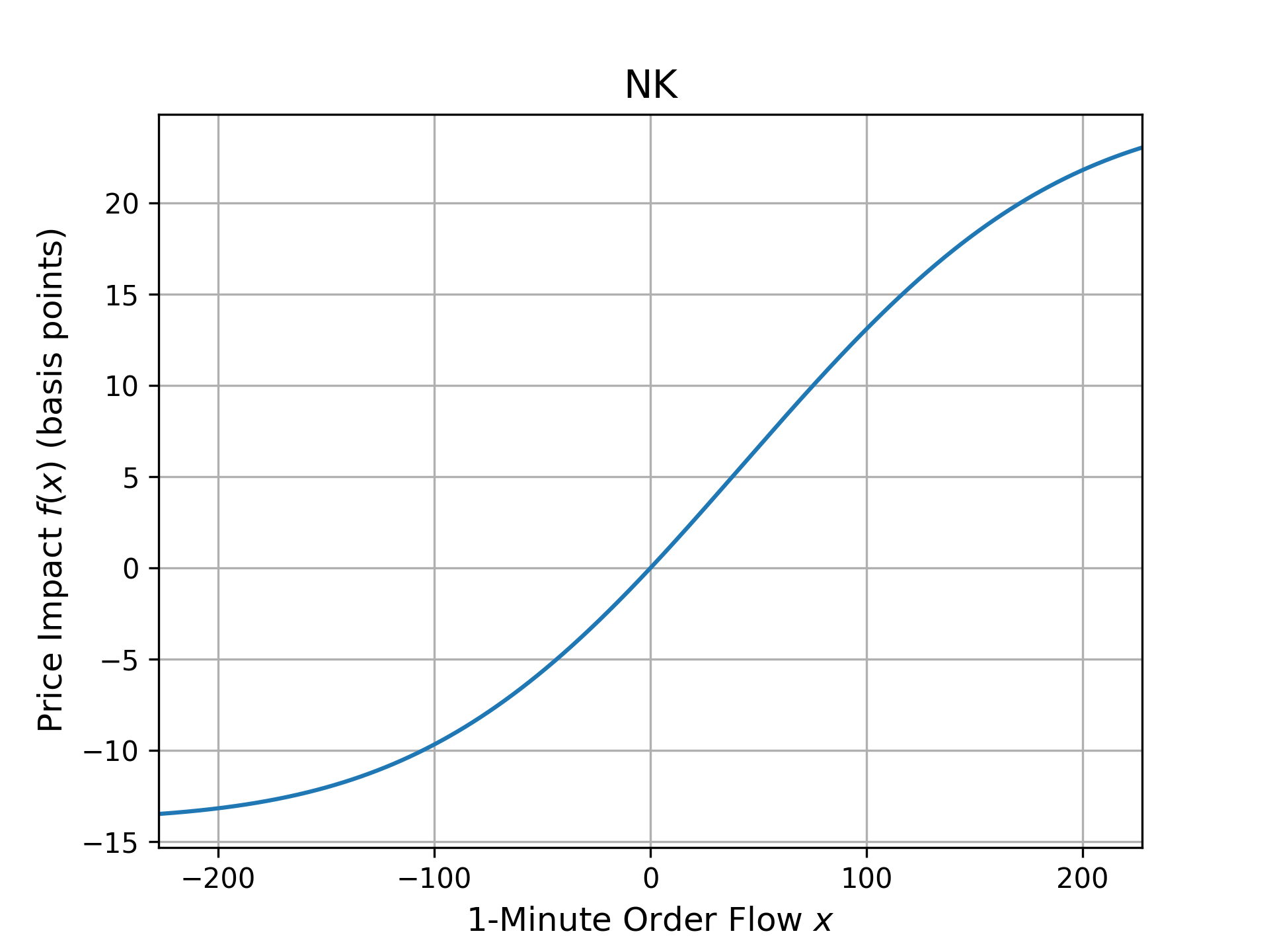
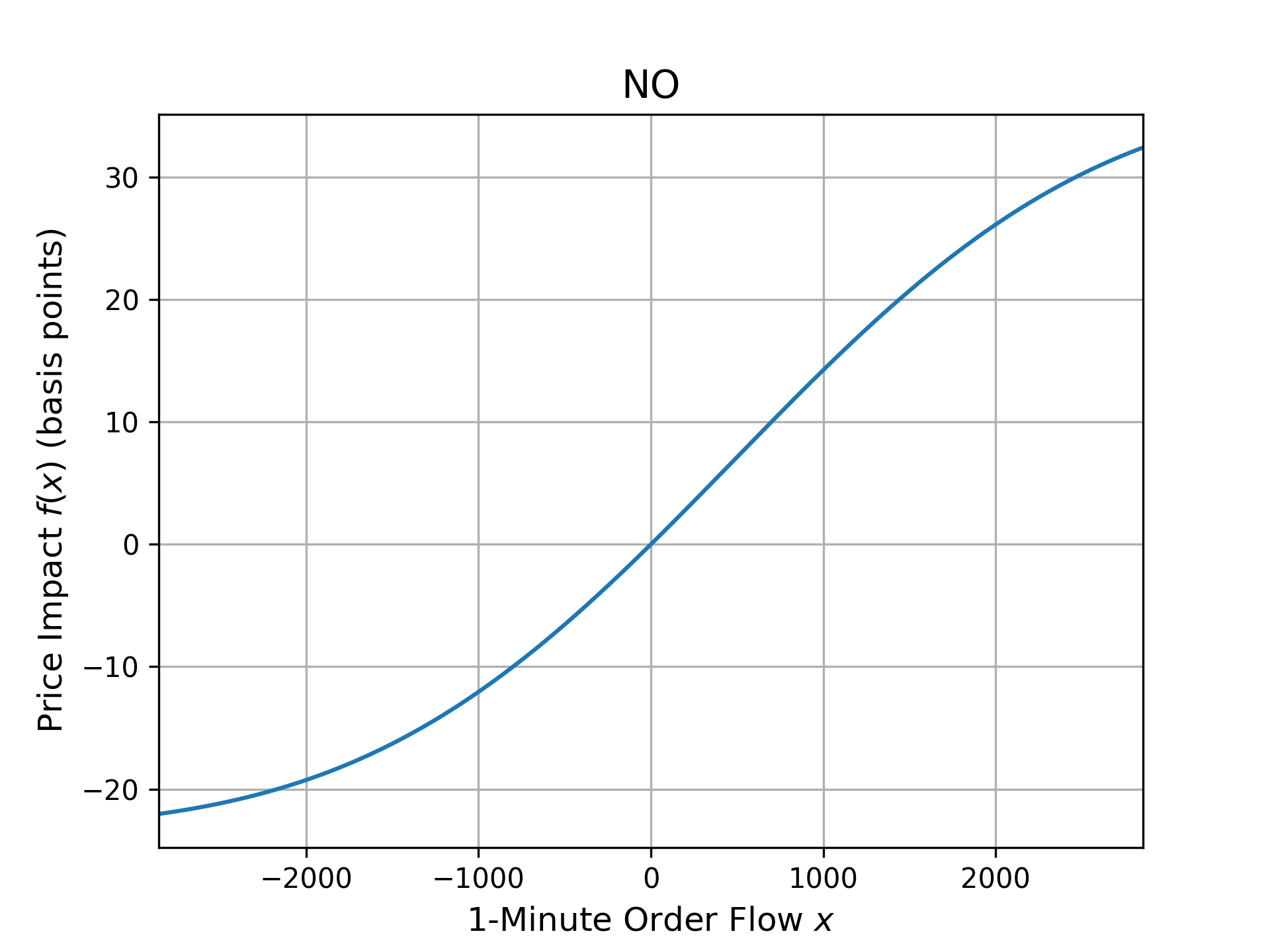
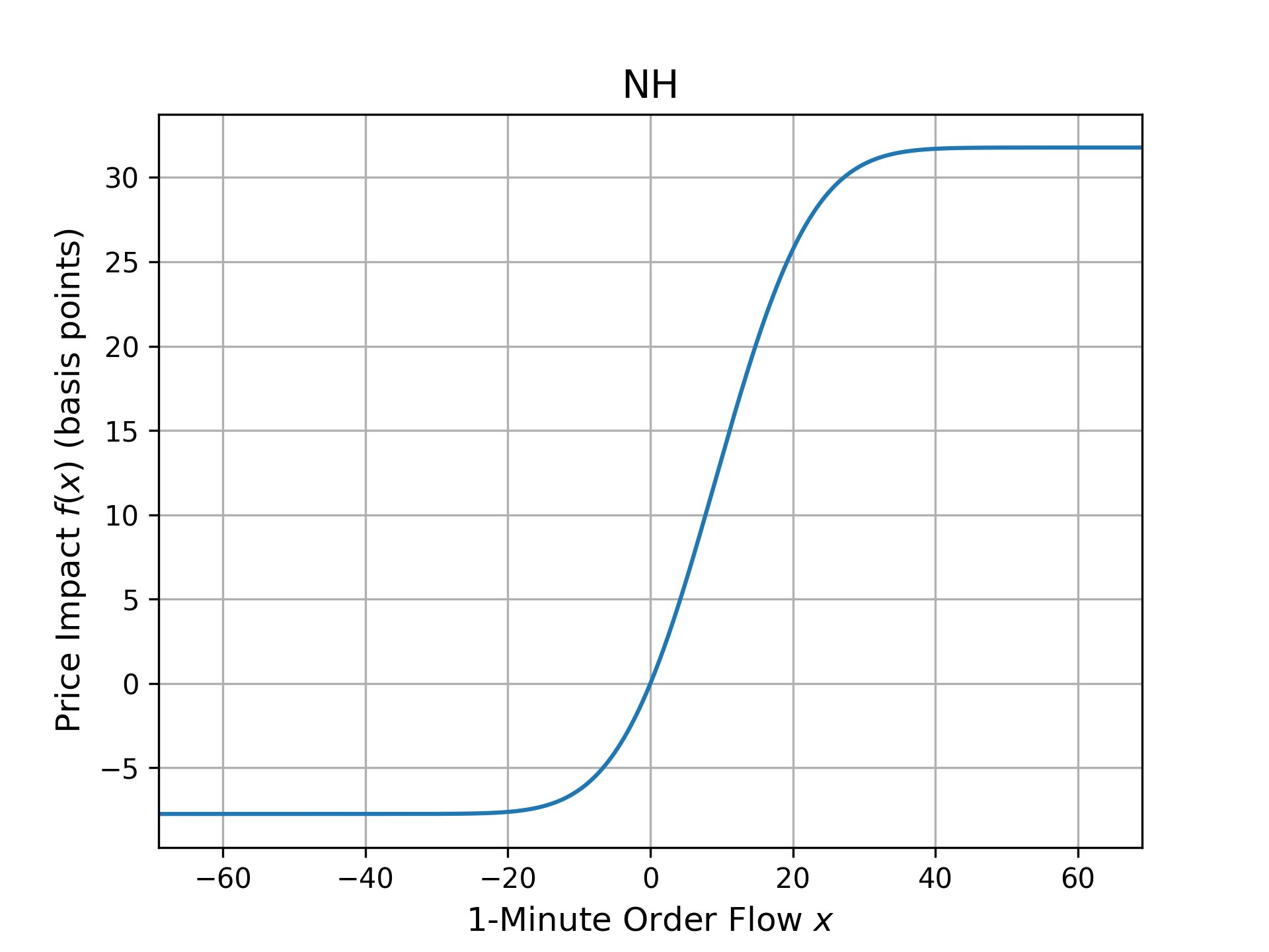
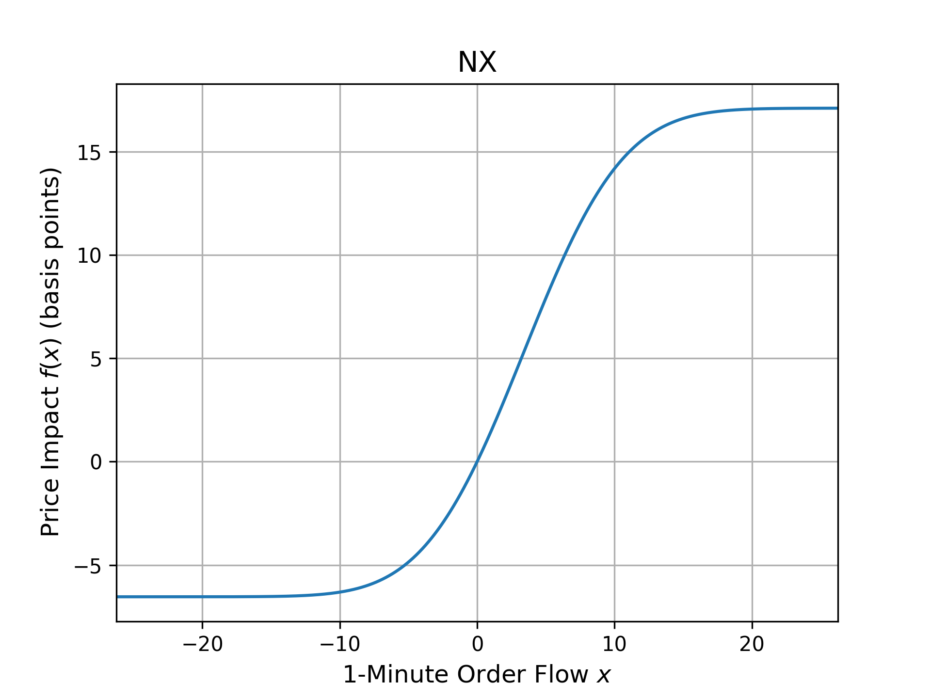
Figure 2: Price Impact Functions of Four Futures on 15 June 2016.

Figure 2 shows the 4 impact functions plotted with the respective sets of estimated parameters, i.e., $\widehat{\ell},\widehat{p}$, and $\widehat{q}$. Clearly, we see that they are all S-shape curves. It is interesting to note the asymmetry with respect to $x=0$. When $\widehat{p}$ is estimated to be positive, negative order flow has a larger impact than positive order flow of the same trade size, and vice versa. This asymmetry is captured by Proposition 4.2 as a result of the concave and convex nature of our $f(x)$ with respect to an inflection point, which is not at $x=0$. From Table 2, we see that all the $p$ estimates are negative, and in Figure 2, it is evident that the price impact of $x>0$ is asymmetrically larger on that particular day.

This asymmetry of buys versus sells could be due to the fact that the futures price was moving higher on that day. In line with this fact, Table 2 shows that all the drift estimates—intrinsic to the true price primarily—are positive. It must be that there were more aggressive buy orders willing to pay for the price impact cost, pushing the price higher as a result.

Figure 2 is about here.

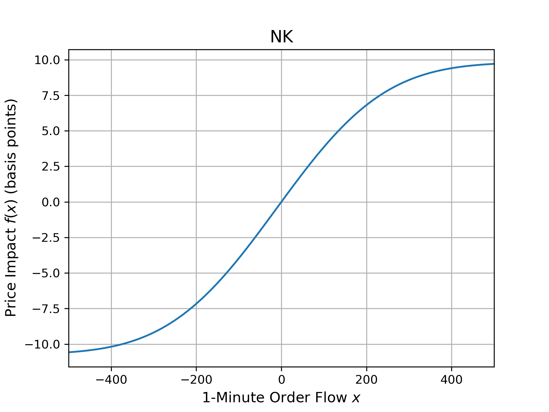
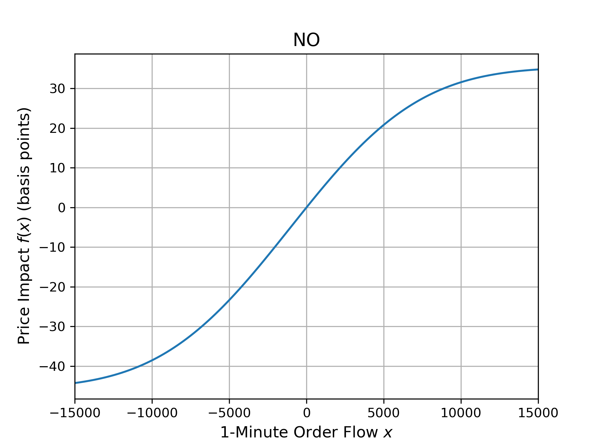
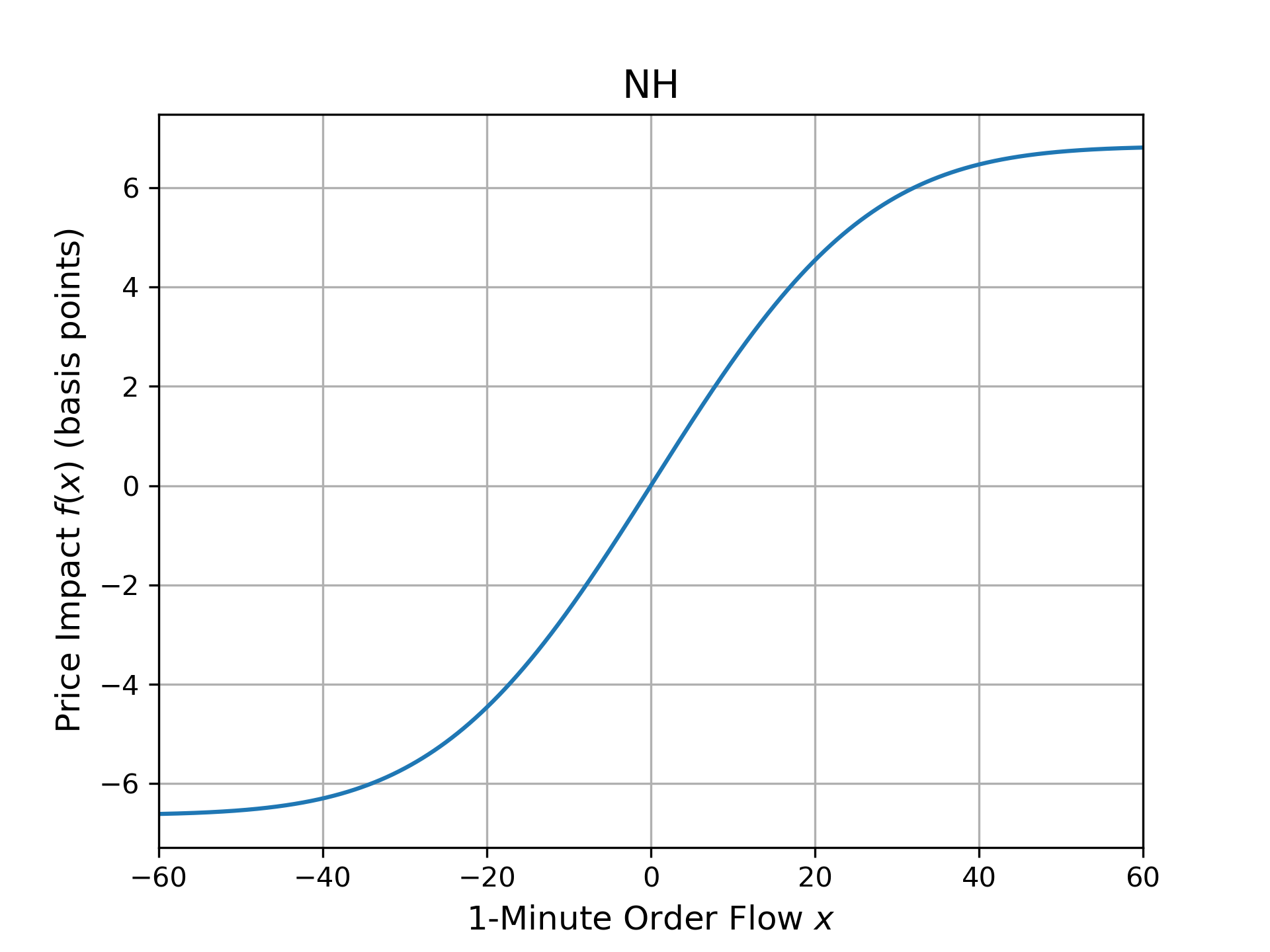
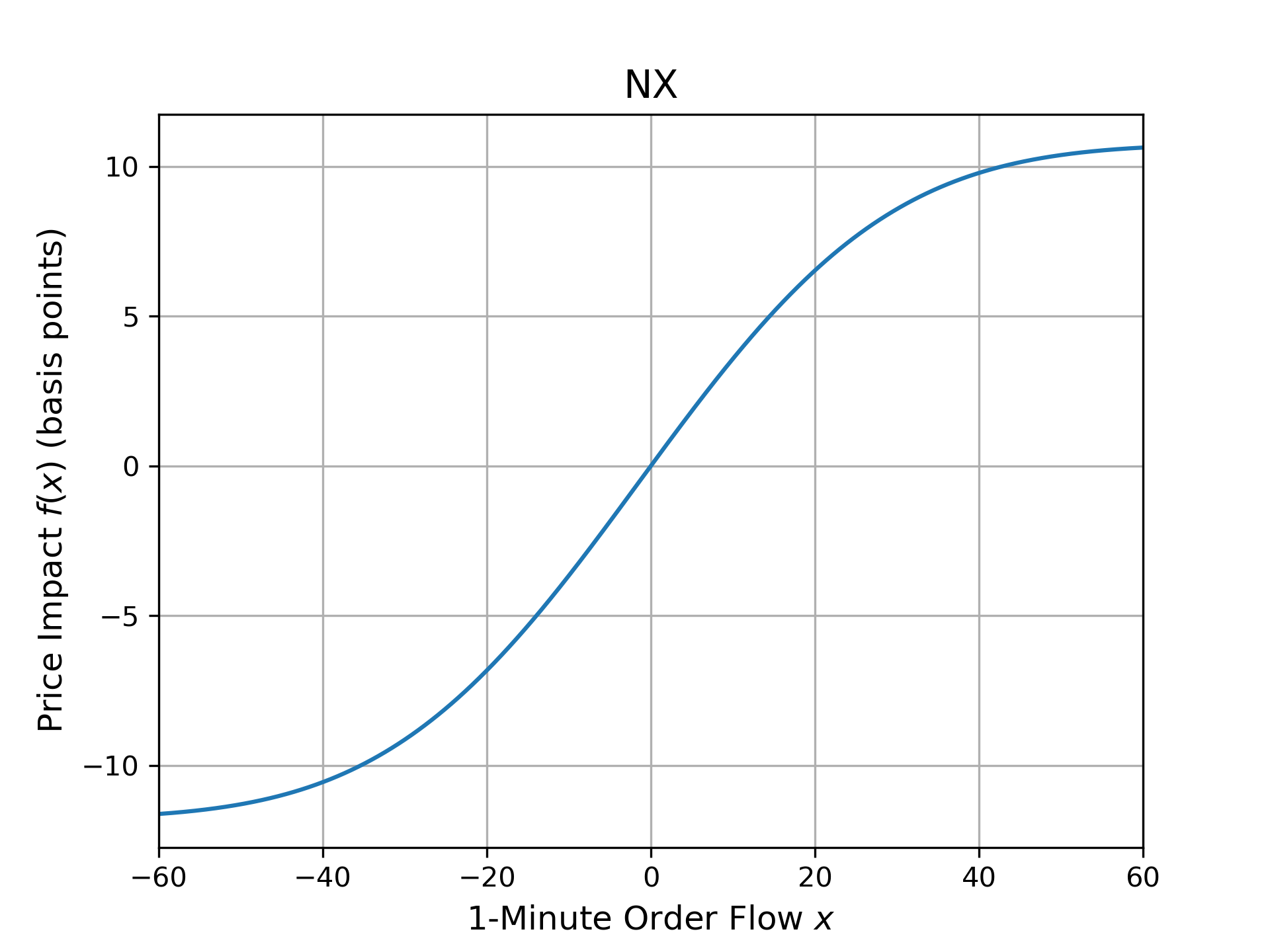
Figure 3: Price Impact Functions of Four Futures Estimated over the Entire Sample Period.

The asymmetry in the S-shape price impact function may occur on a given single day as shown in Figure 2. But would the asymmetry persist if we consider all the trading days over the entire sample period? To answer this question, we pool together all the order flows and the corresponding logarithmic returns, and run the same constrained nonlinear regression. The overall looks of the four S-shape functions estimated respectively with pooled data from the entire sample period are displayed in Figure 3.

Figure 3 is about here.

We find that the S-shape impact functions for offshore NH and NX futures in Figure 3 are much more symmetric compared to the corresponding pairs in Figure 2. The price impact functions have a range of about $\pm$6 basis points for NH futures and $\pm$10 basis points for NX futures. The onshore big Nikkei NK in Figure 3 is more symmetric too, with the range of price impacts being approximately $\pm$10 basis points for the order flows of $\pm$400 contracts. To a lesser extent has the mini Nikkei NO in Figure 3 become symmetric, with buys being about 30 basis points for a large buy order flow of 10,000 contracts and about 40 basis points for a large sell order flow of the same size. For its single-day counterpart in Figure 2, the difference of 10 basis points already starts to appear at only $\pm$3,000 contracts.

5.4 Discussion of Estimation Results

Recall that the parameter $\ell$ in the S-shape function can be regarded as Kyle’s illiquidity measure $\lambda$. It is the price impact cost in basis points per unit of $\Phi(x)$ as in (4.68), i.e., when $\Phi(x)=1$. Looking at the $\ell$ estimates in Table 2, it is clear that JPX’s mini futures (NO) has the least value with only 0.01 basis points. This outcome intuitively makes sense because mini futures is the most heavily traded among the 4 contracts. Overall, we observe that the two futures of JPX are more liquid than CME’s offshore futures during the Asian hours of trading, as anticipated.

Next, notice that in Table 2, the order of magnitude for the $p$ and $q$ across different Nikkei 225 futures is different. In particular, $p$ and $q$ are the smallest for JPX’s mini futures. By contrast, $\widehat{a}$, which is exclusively about the unobservable trice price $S_{t}$ since $\displaystyle a=\mu_{S}-\sigma_{S}^{2}/2$, is more or less equal across the 4 futures. This result is consistent with the fact that these 4 futures are written on the same underlying equity index, and therefore their unobservable prices $S_{t}$ should move in tandem generally with the underlying index. This result provides evidence that our modeling and econometrics are on the right track.

Table 3 is about here.

Now, in Table 3, we report the estimation results for each of the 4 futures contracts when the order flows and the corresponding log returns in the entire sample period of about 3 years and 7 months are pooled together. Their overall S-shape curves have already been plotted in Figure 3.

First, we find that the parameter estimates in Table 3 are smaller than the corresponding estimates in Table 2, by one to two orders of magnitude. This finding is to be expected because when one considers intra-day data over many days, one will find that the overall negative order flows and the overall positive order flows tend to counteract each other. If for a certain intra-day time period in a trading day, the order flow is a big positive and for another time period in another trading day, the order flow is a big negative, then there is a higher likelihood that they both occur and thus balance out each other in the nonlinear regression.

Second, despite the smaller parameter estimates, their $t$ statistics are however larger by comparison with Table 2 in general. The main exception is the $t$ statistics for the drift $\widehat{a}$, which are compatible with the single-day $t$ statistics. The adjusted $R^{2}$ are lower in Table 3. This is because the number of pairs of the order flow and the log return has become a lot larger (about a thousand times) in the pooled regression. Extreme large order flows and log returns are more likely to occur, which tend to make the residual sum of squares larger, resulting in a lower adjusted $R^{2}$.

Interestingly, the findings from the single-day results are also observed in multi-day Table 3. Again, we find that $\widehat{a}$’s estimates (after multiplied by $10^{6}$) of 1.04, 1.05, 1.01, and 1.00 are numerically compatible across the 4 futures contracts. As mentioned earlier, this compatibility must occur because these 4 futures contracts are written on the same underlying Nikkei 225 index, and they should move in the same direction at almost the same drift rate. As anticipated, we find that NO futures contract is the most liquid with the smallest $\widehat{\ell}$, $\widehat{p}$, and $\widehat{q}$ estimates. The offshore NX futures contract, which is denominated in US dollars, is the least liquid overall during the Asian trading hours.

In summary, the findings from Tables 2 and 3, are consistent with the stylized facts about these 4 Nikkei 225 index futures traded concurrently during the Asian hours. As anticipated, the mini futures is most liquid, and CME’s futures are comparatively less liquid. Moreover, the drift rate $a$, being primarily about the spot Nikkei 225 index that is common to and shared by these 4 futures, is more or less equal statistically, despite the fact that their liquidity levels differ significantly.

5.5 Comparisons

Now we present a comparison of the heuristic function against our linear and S-shape functions in capturing the price impact. Table 4 displays the adjusted $R^{2}$ to examine the goodness of fit, and the Bayesian information criterion (BIC) to evaluate over-fitting vis-à-vis under-fitting.

A point to note is that for the S-shape function, as discussed previously, as in (4.68), the parameter $\ell$ plays a role that is analogous to the $\alpha$ parameter in the heuristic and linear functions.

Again, we note that the drift parameter $a$ has quantitatively similar estimate $\widehat{a}$, which is not statistically significant at the 5% level. By contrast, the $\alpha$ estimates are all statistically significant, and their values are rather different. In particular, the $\alpha$ estimate is the smallest for our linear function, being of an order of magnitude smaller than the corresponding estimates for the heuristic and the S-shape function. Overall, as expected, JPX’s NO futures has the smallest $\widehat{\alpha}$, and CME’s NX futures has the largest $\widehat{\alpha}$ during the Asian trading hours.

More importantly, we find that the adjusted $R^{2}$ for the S-shape function is higher than those of linear and heuristic functions. Also the residual sum of squares is the least by comparison. Therefore, we have evidence that the S-shape function fits the data better. From the Bayesian information criterion (BIC), we see that the 3-parameter S-shape function has s much lower BIC compared to those of 1-parameter heuristic and linear functions, which means that over-fitting by 3 parameters did not occur.

Table 4 is about here.

5.6 All Estimations

Now, we examine whether the evidence from a single day (15 June 2016) presented earlier does hold for the entire set of estimates. From the beginning of November 2013 through early June 2017 for a total of 885 days for JPX’s onshore futures and 927 days for CME’s offshore futures, we obtain by (5.71) a set of $\ell,p$ and $q$ estimates and other statistics from the 1-minute intra-day data for each day.

We run the paired sample tests of their adjusted $R^{2}$ for each trading day in our sample period. The paired $t$ test results in Panel A of Table 5 shows that the heuristic square-root function in general has a better fit with the data than the linear function, with the exception of JPX’s mini futures contract (NO). On average, the adjusted $R^{2}$ of the linear function is about 3.16 percentage points lower than that of the heuristic function in the case of CME’s NH futures, and the $t$ statistic of -28.53 suggests that this difference is highly significant. In a way, it could be the reason why the industry uses the square-root function rather than the linear function in their analysis of price impact.

Panel B of Table 5 shows the $t$ test results for comparing the residual sum of squares (RSS). For NK and NH futures contracts, the $t$ statistics are significant and we can conclude that for our samples, the linear function has larger errors in fitting the data compared to the heuristic function. For NX futures, however, the difference in RSS is not significant. On the other hand, for NO futures, our linear function’s RSS is significantly smaller than that of the heuristic function.

More importantly, the $t$ test statistics for the comparison between our S-shape function and the heuristic function indicate that for all 4 futures contracts, the differences in adjusted $R^{2}$ and RSS are statistically significant. For the onshore NK and NO contracts, the S-shape function is better than the heuristic function by 2.08 and 2.92 percentage points, respectively. For the off-shore NH and NX contracts, the difference is about 1.5 percentage points. The RSS incurred by our S-shape function is much smaller. Also, given that the BIC is on average smaller than the BIC for the single-parameter heuristic function by 1,000, our 3-parameter S-shape function does not have the problem of over-fitting. The empirical evidence points to the finding that our S-shape price impact function is more capable in reflecting the price impact of a Nikkei futures trade.

Table 5 is about here.

Next, we compare the liquidity of the 4 futures contracts on the same underlying equity index. For this purpose, in Table 6, we provide the descriptive statistics for the parameter estimates of the S-shape functions over the sample period. The average and standard deviation, along with the percentiles, are tabulated. We note that the distributions of the parameter estimates are skewed to the right, so much so that the average and the 50-th percentile (median) are quite different.

For the $\ell$ parameter estimates, which mirrors the role of $\lambda$ parameter in Kyle (1985), we find that, as anticipated, the NO futures is the most liquid as its average of 0.10 basis points (bps) is the smallest. Moreover, for each percentile in Table 6, NO futures’ $\ell$ estimate is the smallest among the 4 futures contract specifications. As shown in (4.68), a small $\ell$ leads to a small disparity or spread from the true price, and vice versa.

By contrast, based on the percentiles, the dollar-denominated NX futures is the least liquid during Asian trading hours, since its $\ell$ estimates are the largest for each percentile in Table 6 up to the median value of 0.49 basis points. Beyond the 90-th percentile, JPX’s big Nikkei futures NK is the least liquid. This empirical finding is consistent with the fact that the minimum tick size of NK futures is twice that of all the other 3 futures contracts. Furthermore, the contract size of NK futures is 10 times that of NO futures and twice that of NH futures. It is a stylized fact that in market microstructure, a larger tick size and contract size will lead to a larger quoted spread, everything else being equal.

Table 6 is about here.

Finally, it is interesting to note that despite the differences in the average $\ell$, $p$, and $q$ estimates, the average inflection points in Table 6 are compatible with the estimates obtained from pooled observations in Table 3.

5.7 Market Depth

The inflection point, defined in (4.60) as primarily a ratio of $p$ and $q$, may be interpreted as the market depth in relation to the market price movement. By construction, the inflection point is in the unit of order flow (number of contracts). For our S-shape function, the unique inflection point is the order flow at which the gradient of the function is at its maximum, which means that the price impact from the order flow is at its highest. Thus, if the inflection point is far away from the origin, it means that a larger volume of order flow is needed to create the maximum impact. Put differently, the market is deep enough to ameliorate the price impact from small- to medium-sized order flows.

Interestingly, according to (4.67), the inflection point is dependent on 2 parameters of the market price of liquidity risk ($\delta$ and $\tau$), 3 quantities of the order flow ($c$, $m$, and $\eta$), and the volatility $\sigma_{S}$ of the true price return through its correlation $\rho$ with the order flow. As a matter of fact, almost all the parameters in our framework appear in the calculation of the inflection point.

As anticipated, the mini futures NO with the smallest contract size has the largest inflection point in absolute value. In Table 6, NO futures has an average inflection point of -1,654 contracts. Coming in second is NK futures with an average of 28 contracts. Obviously during the Asian trading hours, JPX’s onshore futures are more active and the market depth is relatively deeper than the offshore futures with an average of 3 contracts only.

Table 7 is about here.

Now, it is well known that market depth is intrinsically related to the amount of liquidity in the (electronic) market, i.e., the numbers of contracts waiting to buy and to sell. Our data sets contain (only) the best bid and best offer prices along with their respective sizes. In Table 7, we present the descriptive statistics of the best bid and ask sizes at the beginning of each 1-minute interval. It is evident that NO futures have the largest bid and ask sizes of 332 and 341 contracts on average, respectively, over our sample period of about 3 years and 7 months. The big Nikkei NK Futures comes in second. Understandably, during the Asian trading hours, the offshore NH and NX futures of CME have rather thin liquidity of less than 10 contracts. The statistics in 7 provide collaborative evidence based on futures’ best quotes. They support the idea that the inflection point of the S-shape function may be conceived as a measure for market depth.

6 Conclusions

Starting from the framework in Çetin et al. (2004), we introduce the key proposition that the order flow is a mean reversion process. Applying Itô’s calculus, and with a change of probability measure involving the market price of market risk and the market price of liquidity risk, we obtain an inhomogeneous Bernoulli differential equation. By solving the equation in two special cases, we obtain two closed-form solutions for the functional form of the price impact function. The first case yields a linear impact function that is consistent with Kyle (1985), and the second case produces a nonlinear S-shape function.

Within our mathematical framework, we explore the theoretical implications for a possible explanation of the phenomenon that the volatility is stochastic. In principle, order flow may drive the price temporarily above or below the unobservable fundamental value. In other words, order flow as a manifestation of trading will give rise to additional volatility that is otherwise absent. This excess volatility is stochastic because the order flow is stochastic.

Our theoretical paper also includes an empirical study. Using 4 different futures contracts of different specifications but on the same underlying Nikkei 225 index, we find that the estimates from constrained nonlinear least squares method are consistent with the stylized facts about the liquidity of these futures. We also provide evidence indicative of the superiority of our S-shape function over the heuristic square-root functions. Interestingly, our empirical analysis shows that the inflection point of the S-shape function can be interpreted as the market depth.

Market participants and researchers are interested in estimating the market depth, and the financial implications of price impact. As a possible application of the S-shape price impact function, we show that the notion of market depth can be implemented to capture the level of liquidity risk in trading, much like volatility is a measure of price uncertainty or risk. Another application is to use the price impact function for pre-trade and post-trade analyses to estimate the price impact cost of trading a certain amount of financial instrument. Although our empirical study focuses on Nikkei 225 futures for checking the correctness of our model, our framework is general and potentially applicable to futures on commodity and on interest rates, forex, as well as stocks.

Table 1: Descriptive Statistics of Nikkei 225 Index Futures Contracts

				Daily Average (Contracts)
Name	Bloomberg	Contract	Tick	Volume	Positive	Negative	Order	Volatility of
of Futures	Symbol	Size	Size		OF	OF	Flow (OF)	OF   $\big{(}\widehat{\eta}\big{)}$
JPX Big Nikkei	NK	¥1,000	10	52,368	14,013	13,572	1.23	162.03
JPX Mini Nikkei	NO	¥100	5	441,585	75,377	75,885	-1.41	700.79
CME Nikkei	NH	¥500	5	7,331	1,358	1,420	-0.17	17.22
CME Nikkei	NX	$50	5	3,702	742	768	-0.07	8.62

This table tabulates the 4 futures contracts on the same underlying Nikkei 225 index for 9 AM to 3 PM Japan Standard Time. The sample period is from November 2013 through June 2017, about 3 years and 7 months. The column labeled as “Order Flow (OF)” is the average of 1-minute order flow. Daily average order flow can be inferred from the difference between the positive and negative order flows. The column labeled as “Volatility of OF $\big{(}\widehat{\eta}\big{)}$” contains the volatility estimates for the 1-minute order flows averaged over the sample period.

Table 2: Estimation Results of S-Shape Function of Order Flow on 15 June 2016

	NK	NO	NH	NX
$\widehat{a}\times 10^{5}$	1.97	2.14	2.34	2.11
$t\big{(}\widehat{a}\big{)}$	0.59	0.78	0.77	0.69
$\widehat{\ell}$ (in bps)	0.13	0.01	0.97	1.39
$t\big{(}\widehat{\ell}\big{)}$	4.63	5.52	2.76	2.63
$\widehat{p}$ (%)	-0.34	-0.02	-7.06	-10.49
$t\big{(}\widehat{p}\big{)}$	-1.68	-1.36	-1.71	-1.39
$\widehat{q}\times 10^{5}$	8.15	0.04	653.35	3,076.31
$t\big{(}\widehat{q}\big{)}$	2.03	1.76	1.55	1.39
Inflection (Market Depth)	42	478	11	3
Adjusted $R^{2}$ (%)	27.84	38.98	18.40	16.09

One-minute order flows are obtained for each of the 4 futures contracts over the trading session (9 AM to 3 PM Japan Standard Time) on 15 June 2016. These 4 futures are written on the same underlying Nikkei 225 Index. Through a constrained nonlinear least squares procedure, this table presents the parameter estimates $\big{(}\widehat{p},\widehat{q}$, and $\widehat{\ell}\,\big{)}$ of our S-shape price impact function, together with the estimate $\widehat{a}$ for the drift rate intrinsic to the true price. The $t$ statistic is shown beneath each estimate.

Table 3: Estimation Results of S-Shape Function of Order Flow for the Entire Sample Period

	NK	NO	NH	NX
$\widehat{a}\times 10^{6}$	1.04	1.05	1.01	1.00
$t\big{(}\widehat{a}\big{)}$	0.59	0.88	0.87	0.88
$\widehat{\ell}$ (in bps)	0.041	0.005	0.261	0.372
$t\big{(}\widehat{\ell}\big{)}$	59.60	57.48	55.06	63.99
$\widehat{p}$ (in bps)	2.73	0.24	-9.21	23.67
$t\big{(}\widehat{p}\big{)}$	3.49	6.73	-1.15	3.47
$\widehat{q}\times 10^{6}$	24.80	0.02	2,358.20	1,719.63
$t\big{(}\widehat{q}\big{)}$	23.76	11.27	23.14	22.85
Inflection (Market Depth)	-11	-1,037	0	-1
Adjusted $R^{2}$ (%)	5.86	12.31	4.94	6.44

One-minute order flows are obtained for each of the 4 futures contracts over the trading session (9 AM to 3 PM Japan Standard Time) for the entire sample period from early June 2013 through early July 2017. These 4 futures are written on the same underlying Nikkei 225 Index. Through a constrained nonlinear least squares procedure, this table presents the parameter estimates $\big{(}\widehat{p},\widehat{q}$, and $\widehat{\ell}\,\big{)}$ of our S-shape price impact function, together with the estimate $\widehat{a}$ for the drift rate intrinsic to the true price. The $t$ statistic is shown beneath each estimate.

Table 4: Comparison of Heuristic, Linear, and S-Shape Functions

		$\widehat{a}\times 10^{5}$	$t(\widehat{a})$	$\widehat{\alpha}$ (in bps)	$t(\widehat{\alpha})$	Adj $R^{2}$	RSS$\times 10^{5}$	BIC
	Heuristic	1.97	0.58	0.3691	10.62	26.63%	14.37	-4,258
NK	Linear	2.02	0.59	0.0293	7.46	24.41%	14.80	-4,247
	S-Shape	1.97	0.59	0.1308	4.63	27.84%	14.06	-5,273
	Heuristic	2.13	0.71	0.1457	14.07	36.35%	10.08	-4,385
NO	Linear	2.14	0.71	0.0046	13.49	38.02%	9.82	-4,395
	S-Shape	2.14	0.78	0.0139	5.52	38.98%	9.62	-5,409
	Heuristic	2.26	0.69	0.5411	7.23	14.93%	12.17	-4,318
NH	Linear	2.27	0.69	0.0720	4.14	11.12%	12.72	-4,302
	S-Shape	2.34	0.77	0.9707	2.76	18.40%	11.62	-5,341
	Heuristic	2.12	0.67	0.7265	6.60	14.64%	12.05	-4,321
NX	Linear	2.10	0.66	0.1428	4.96	10.35%	12.66	-4,303
	S-Shape	2.11	0.69	1.3894	2.63	16.09%	11.80	-5,336

This table tabulates a comparison of the heuristic square root, linear, and S-shape functions of order flow in capturing the price impact for the trading session on 15 June 2016 (9 AM to 3 PM Japan Standard Time). The $\ell$ parameter of the S-shape function is used in this comparison with the $\alpha$ parameter in the heuristic and linear functions. $\widehat{a}$ is the estimate of the intercept and $t(\widehat{a})$ is its $t$ statistic, likewise for the Kyle (1985) illiquidity measure $\alpha$. In addition to the adjusted $R^{2}$, we also include the residual sum of squares (RSS) to measure the goodness of fit. The Bayesian information criterion (BIC) shows whether the S-shape function has an over-fitting problem.

Table 5: Two-Sample $t$ Tests of Goodness of Fit

Panel A: Adjusted $R^{2}$

	Linear $-$ Heuristic		S-shape $-$ Heuristic
	mean difference	$t$ statistic	mean difference	$t$ statistic
NK	-2.34%	-20.30	2.08%	15.91
NO	1.44%	11.91	2.92%	26.75
NH	-3.16%	-28.53	1.48%	17.27
NX	-1.60%	-13.08	1.56%	17.48

Panel B: Residual Sum of Squares

	Linear $-$ Heuristic		S-shape $-$ Heuristic
	mean difference $\times 10^{6}$	$t$ statistic	mean difference $\times 10^{6}$	$t$ statistic
NK	2.89	2.51	-7.63	-5.43
NO	-3.65	-3.09	-5.81	-3.59
NH	1.58	3.95	-2.44	-2.07
NX	0.32	0.67	-3.35	-2.28

This table tabulates the results of two-sample $t$ tests. Under the null hypotheses that the adjusted $R^{2}$ is no different in Panel A and the residual sum of squares is no different in Panel B, we test our linear and non-linear price impact functions against the heuristic square root function. This comparison is over the entire sample period from early November 2013 through early June 2017.

Table 6: Descriptive Daily Statistics for S-Shape Price Impact Functions

				Percentile
Estimate	Symbol	Average	STD	1	5	10	50	90	95	99
$\ell$	NK	5.17	16.83	3.3$\times 10^{-5}$	0.01	0.02	0.12	12.78	20.20	84.73
(bps)	NO	0.10	0.63	1.3$\times 10^{-3}$	1.9$\times 10^{-5}$	2.4$\times 10^{-5}$	0.01	0.02	0.26	2.24
	NH	0.93	3.99	0.05	0.08	0.12	0.32	0.94	1.58	13.45
	NX	1.87	12.54	0.09	0.16	0.21	0.49	1.29	2.34	28.86
$p$	NK	-0.28	4.07	-25.98	-2.48	-0.83	1.0$\times 10^{-4}$	0.66	2.11	8.21
	NO	-0.02	0.30	-1.2$\times 10^{-3}$	-4.7$\times 10^{-4}$	-3.1$\times 10^{-4}$	1.2$\times 10^{-5}$	3.4$\times 10^{-4}$	5.1$\times 10^{-4}$	1.2$\times 10^{-3}$
	NH	-0.08	1.54	-1.77	-0.18	-0.07	-3.1$\times 10^{-7}$	0.06	0.12	2.11
	NX	-0.04	0.84	-0.86	-0.13	-0.07	6.1$\times 10^{-7}$	0.07	0.11	0.53
$q$	NK	6.48	13.79	3.0$\times 10^{-9}$	1.1$\times 10^{-6}$	4.1$\times 10^{-6}$	4.9$\times 10^{-4}$	31.24	37.10	55.80
	NO	1.7$\times 10^{-3}$	0.03	7.2$\times 10^{-11}$	4.2$\times 10^{-10}$	1.5$\times 10^{-9}$	2.1$\times 10^{-7}$	1.4$\times 10^{-6}$	2.1$\times 10^{-6}$	7.8$\times 10^{-5}$
	NH	0.96	6.39	5.6$\times 10^{-9}$	7.3$\times 10^{-5}$	2.5$\times 10^{-4}$	4.2$\times 10^{-3}$	0.06	0.23	40.30
	NX	0.49	4.97	5.0$\times 10^{-9}$	3.5$\times 10^{-6}$	2.9$\times 10^{-4}$	0.01	0.07	0.17	3.91
Inflection	NK	28	3,136	-1,615	-281	-137	-0.02	123	276	7,749
Point	NO	-1,654	40,868	-137,606	-75,000	-3,988	-46	3,919	43,923	132,584
(contracts)	NH	-3	267	-199	-42	-19	0.03	21	48	323
	NX	-3	272	-961	-39	-17	-0.01	17	42	792
Adjusted	NK	15.71	8.12	1.72	3.77	5.89	15.27	26.39	29.18	35.05
$R^{2}$	NO	28.80	8.57	10.07	14.22	17.19	29.44	39.15	41.29	47.32
(%)	NH	15.19	5.67	3.77	6.68	8.36	14.85	22.61	25.03	28.69
	NX	17.71	5.70	5.68	8.68	10.52	17.44	25.22	27.20	32.06

The parameter estimates of the S-shape function are obtained by a constrained nonlinear least squares procedure on 1-minute data, which are processed from Bloomberg’s tick data. The sample period is from early November 2013 to early June 2017, for a total of 885 days for JPX’s onshore futures (NK and NO) and 927 days for CME’s offshore futures (NH and NX). A set of parameter estimates is obtained for each trading day in the sample period, along with the inflection point and the adjusted $R^{2}$. We report the daily average, standard deviation (STD), and the percentiles.

Table 7: Descriptive Statistics of Best Bid and Ask Sizes

				Percentile
		Average	STD	1	5	10	50	90	95	99
NK	Bid Size	125	44	49	64	73	119	184	208	252
	Ask Size	127	45	51	63	73	122	186	209	266
NO	Bid Size	332	119	111	160	193	327	477	559	668
	Ask Size	341	128	110	165	193	330	506	575	720
NH	Bid Size	8	3	3	4	5	7	12	14	18
	Ask Size	8	3	2	4	4	8	12	14	18
NX	Bid Size	7	3	2	3	4	6	10	12	15
	Ask Size	7	3	2	3	4	7	10	13	15

From Bloomberg’s tick data, we identify the best bid and ask sizes at the beginning of each 1-minute interval for each trading session from 9 AM to 3 PM Japan Standard Time. The sample period is from early November 2013 to early June 2017, for a total of 885 days for JPX’s onshore futures (NK and NO) and 927 days for CME’s offshore futures (NH and NX). Daily average bid and ask sizes are computed and the table presents the descriptive statistics for the sample period with “std” denoting the standard deviation.

Figure 1: One-Minute Order Flows of Four Futures on 15 June 2016.

Panel A: JPX’s Nikkei 225 Large Contract (NK)

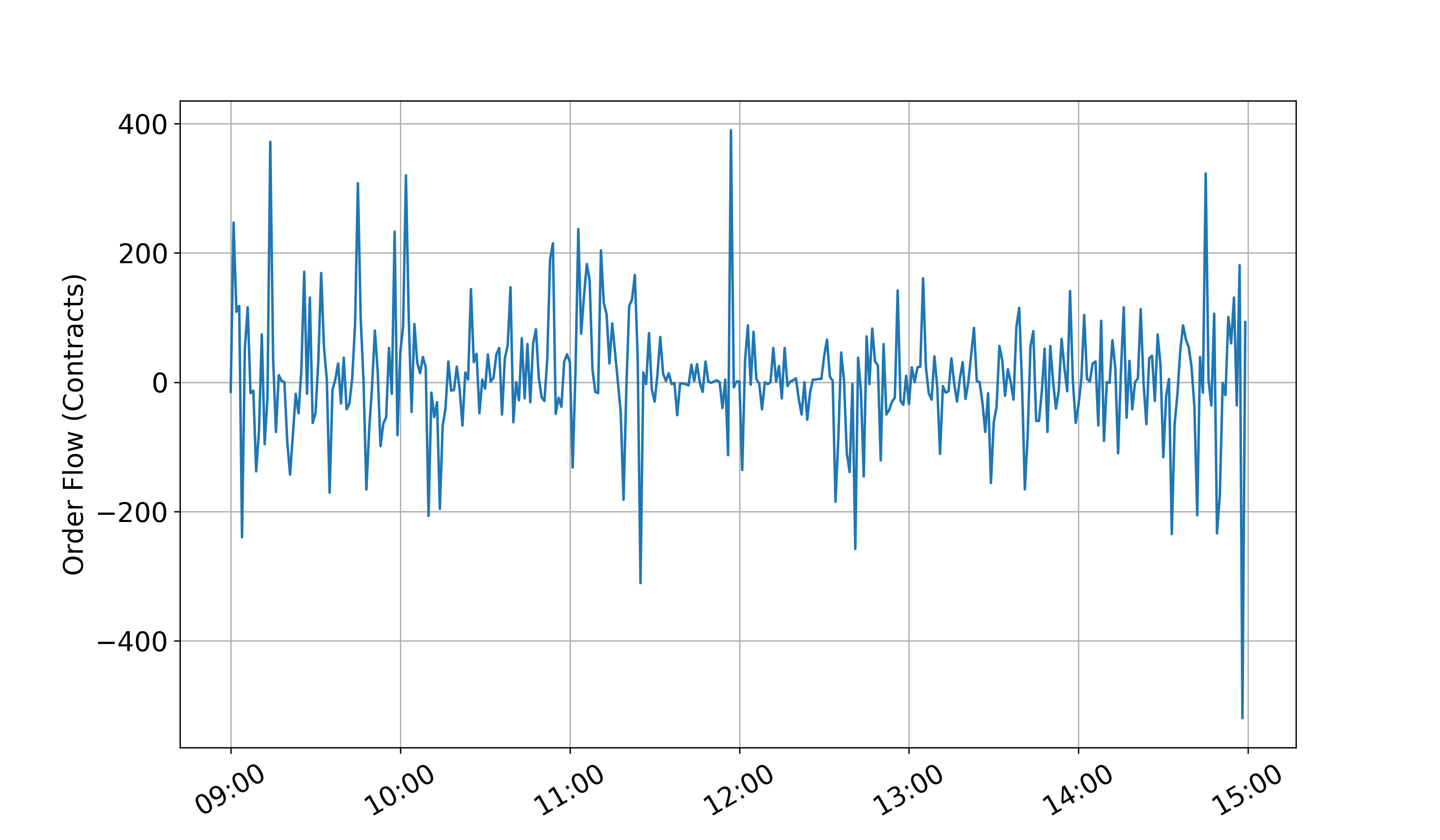
Panel B: JPX’s Nikkei 225 Mini Contract (NO)

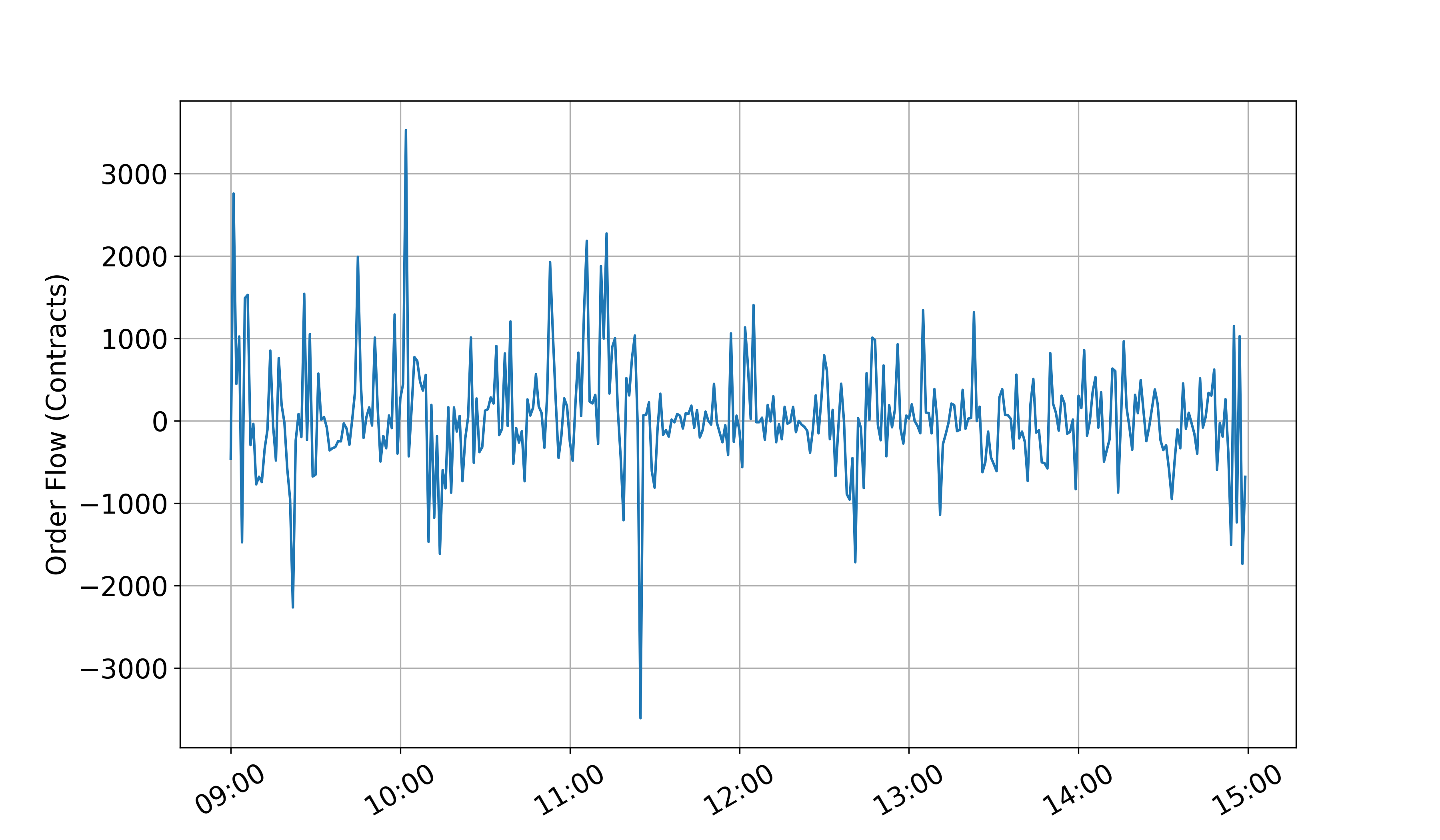
Panel C: CME’s Nikkei 225 Yen-Denominated Contract (NH)

Panel D: CME’s Nikkei 225 Dollar-Denominated Contract (NX)

References

- (1)
- Acharyaa and Pedersen (2005) Acharyaa, V. V. and Pedersen, L. H. (2005). Asset pricing with liquidity risk, Journal of Financial Economics 77: 375–410.
- Almgren (2012) Almgren, R. (2012). Optimal trading with stochastic liquidity and volatility, SIAM Journal of Financial Mathematics 3: 163–181.
- Almgren and Chriss (2000) Almgren, R. and Chriss, N. (2000). Optimal execution of portfolio transactions, Journal of Risk 3(2): 5–39.
- Amihud (2002) Amihud, Y. (2002). Illiquidity and stock returns: Cross section and time-series effects, Journal of Financial Markets 5: 31–56.
- Asai and Michael (2000) Asai, M. and Michael, M. (2000). Forecasting the volatility of Nikkei 225 futures, Journal of Futures Markets 37(11): 1141–1152.
- Bouchaud (2010) Bouchaud, J.-P. (2010). Price impact, in R. Cont (ed.), Encyclopedia of Quantitative Finance, Vol. 3, John Wiley and Sons, pp. 1402–1407.
- Bouchaud et al. (2009) Bouchaud, J.-P., Farmer, J. D. and Lillo, F. (2009). How markets slowly digest changes in supply and demand, in T. Hens and K. R. Schenk-Hoppé (eds), Handbook of Financial Markets: Dynamics and Evolution, Elsevier, chapter 2, pp. 57–160.
- Çetin et al. (2004) Çetin, U., Jarrow, R. A. and Protter, P. (2004). Liquidity risk and arbitrage pricing theory, Finance and Stochastics 8(3): 311–341.
- Chan and Fong (2000) Chan, K. and Fong, W.-M. (2000). Trade size, order imbalance and the volatility-volume relation, Journal of Financial Economics 57: 247–273.
- Chordia et al. (2017) Chordia, T., Hu, J., Subrahmanyam, A., and Tong, Q. (2017). Order Flow Volatility and Equity Costs of Capital, Management Science, Accepted paper to appear.
- Dai et al. (2016) Dai, M., Li, P., Liu, H. and Wang, Y. (2016). Portfolio choice with market closure and implications for liquidity premia, Management Science 62(2): 368–386.
- Evans and Lyons (2002) Evans, M. D. D. and Lyons, R. K. (2002). Order flow and exchange rate dynamics, Journal of Political Economy 110(1): 170–180.
-
Ferraris (2008)
Ferraris, A. (2008).
Equity Market Impact Models, Deutsche Bank AG.
http://dbquant.com/Presentations/Berlin200812.pdf - Frijns and Tse (2015) Frijns, B. and Tse, Y. (2015). The informativeness of trades and quotes in the FTSE 100 Index futures market, Journal of Futures Markets 35: 105–126.
-
Gatheral et al. (2012)
Gatheral, J., Schied, A. and Slynko, A. (2012).
Transient linear price impact and Fredholm integral equations, Mathematical Finance 22(3): 445–474.
http://dx.doi.org/10.1111/j.1467-9965.2011.00478.x - Gerig (2007) Gerig, A. N. (2007). A Theory for Market Impact: How Order Flow Affects Stock Price, PhD thesis, Graduate College of the University of Illinois at Urbana-Champaign.
- Hasbrouck (2004) Hasbrouck, J. (2004). Liquidity in the Futures Pits: Inferring Market Dynamics from Incomplete Data, Journal of Financial and Quantitative Analysis 39(2): 305–326.
- Huang and Stoll (1997) Huang, R. D. and Stoll, H. R. (1997). The components of the bid-ask spread: A general approach, Review of Financial Studies 10: 995–1034.
- Huang and Ting (2008) Huang, R. and Ting, C. (2008). A functional approach to the price impact of stock trades and the implied true price, Journal of Empirical Finance 15: 1–16.
- Kennedy et al. (2009) Kennedy, J. S., Forsyth, P. A. and Vetzal, K. R. (2009). Dynamic hedging under jump diffusion with transaction costs, Operations Research 57(3): 541–559.
- Kyle (1985) Kyle, A. S. (1985). Continuous auctions and insider trading, Econometrica 53: 1315–1335.
- Liu and Yong (2005) Liu, H. and Yong, J. (2005). Option pricing withan illiquid underlying asset market, Journal of Economic Dynamics and Control 29: 2125–2156.
- Love and Payne (2008) Love, R. and Payne, R. (2008 ). Macroeconomic News, Order Flows, and Exchange Rates, Journal of Financial and Quantitative Analysis 43: 467–488.
- Lyons (2001) Lyons, R. K. (2001). The microstructure approach to exchange rates, MIT Press, Cambridge, Massachusetts.
- Madhavan et al. (1997) Madhavan, A., Richardson, M. and Roomans, M. (1997). Why do security prices change? A transaction-level analysis of NYSE stocks, Review of Financial Studies 10: 1035–1064.
- Perold (1988) Perold, A. F. (1988). The implementation shortfall: Paper versus reality, Journal of Portfolio Management 14: 4–9.
- Roll (1984) Roll, R. (1984). A simple implicit measure of the effective bid-ask spread in an efficient market, Journal of Finance 39: 1127–1139.
- Torre and Ferrari (1999) Torre, N. G. and Ferrari, M. J. (1999). The market impact model, Technical report, BARRA, Inc.
-
Wilinski et al. (2015)
Wilinski, M., Cui, W., Brabazon, A. and Hamill, P. (2015).
An analysis of price impact functions of individual trades on the
London stock exchange, Quantitative Finance 15(10): 1727–1735.
http://dx.doi.org/10.1080/14697688.2015.1071077