SG-VAE: Scene Grammar Variational Autoencoder to generate new indoor scenes

Abstract

Deep generative models have been used in recent years to learn coherent latent representations in order to synthesize high-quality images. In this work, we propose a neural network to learn a generative model for sampling consistent indoor scene layouts. Our method learns the co-occurrences, and appearance parameters such as shape and pose, for different objects categories through a grammar-based auto-encoder, resulting in a compact and accurate representation for scene layouts. In contrast to existing grammar-based methods with a user-specified grammar, we construct the grammar automatically by extracting a set of production rules on reasoning about object co-occurrences in training data. The extracted grammar is able to represent a scene by an augmented parse tree. The proposed auto-encoder encodes these parse trees to a latent code, and decodes the latent code to a parse tree, thereby ensuring the generated scene is always valid. We experimentally demonstrate that the proposed auto-encoder learns not only to generate valid scenes (i.e. the arrangements and appearances of objects), but it also learns coherent latent representations where nearby latent samples decode to similar scene outputs. The obtained generative model is applicable to several computer vision tasks such as 3D pose and layout estimation from RGB-D data.

1 Introduction

Recently proposed approaches for deep generative models have seen great success in producing high quality RGB images [7, 16, 17, 24] and continuous latent representations from images [12]. Our work aims to learn coherent latent representations for generating natural indoor scenes comprising different object categories and their respective appearances (i.e. pose and shape). Such a learned representation has direct use for various computer vision and scene understanding tasks, including (i) 3D scene-layout estimation [27], (ii) 3D visual grounding [3, 31], (iii) Visual Question Answering [1, 18], and (iv) robot navigation [19].

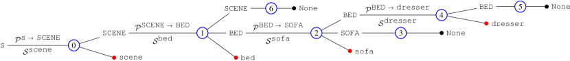
Figure 1: An example of parse tree obtained by applying the CFG to a scene comprising bed, sofa, dresser. The sequence of production rules \raisebox{-0.5pt}{\scriptsize0}⃝-\raisebox{-0.5pt}{\scriptsize6}⃝ are marked in order. The attributes of production rules are displayed above and below of the rules.

Developing generative models for such discrete domains has been explored in a limited number of works [9, 23, 34]. These works utilize prior knowledge of indoor scenes by manually defining attributed grammars. However, the number of rules in such grammars can be prohibitively large for real indoor environments, and consequently, these methods are evaluated only on synthetic data with a small number of objects. Further, the Monte Carlo based inference method can be intractably slow: up to 40 minutes [23] or one hour [9] to estimate a single layout. Deep generative models for discrete domains have been proposed in [6] (employing sequential representations) and in [14] (based on formal grammars). In our work, we extend [14] by integrating object attributes, such as pose and shape of objects in a scene. Further, the underlying grammar is often defined manually [14, 23], but we propose to extract suitable grammar rules from training data automatically. The main components of our approach are thus:

• a scene grammar variational autoencoder (SG-VAE) that captures the appearances (i.e. pose and shape) of objects in the same 3D spatial configurations in a compact latent code (Sec 2);

• a context free grammar that explains causal relationships among objects which frequently co-occur, automatically extracted from training data (Sec 3);

• the practicality of the learned latent space is also demonstrated for a computer vision task.

Our SG-VAE is fast and has the ability to represent the scene in a coherent latent space as shown in Sec 4.

2 Deep generative model for scene generation

The proposed method is influenced by the Grammar Variational Autoencoder [14], so we begin with a brief description of that prior art.

The Grammar VAE takes a valid string (in their case a chemical formula) and begins by parsing it into a set of production rules. These rules are represented as 1-hot binary vectors and encoded compactly to a latent code by the VAE. Latent codes can then be sampled and decoded to production rules and corresponding valid strings. More specifically, each production rule is represented by a 1-hot vector of size $N$, where $N$ is the total number of rules, i.e. $N=|\mathcal{R}|$ (where $\mathcal{R}$ is the set of rules). The maximum size $T$ of the sequence is fixed in advance. Thus the scene is represented by a sequence $\mathcal{X}\in\{0,1\}^{N\times T}$ of 1-hot vectors (note that when fewer than $T$ rules are needed, a dummy/null rule is used to pad the sequence up to length $T$ ensuring that the input to the autoencoder is always the same size). $\mathcal{X}$ is then encoded to a continuous (low)-dimensional latent posterior distribution $\mathcal{N}(\bm{\mu}(\mathcal{X}),\bm{\Sigma}(\mathcal{X}))$. The decoding network, which is a recurrent network, maps latent vectors to a set of unnormalized log probability vectors (logits) corresponding to the production rules. To convert from the output logits to a valid sequence of production rules, each logit vector is considered in turn. The max output in the logit vector gives a 1-hot encoding of a production rule, but only some sequences of rules are valid. To avoid generating a rule that is inconsistent with the rules that have preceded it, invalid rules are masked out of the logit and the max is taken over only unmasked elements. This ensures that the Grammar VAE only ever generates valid outputs. Further details of the Grammar VAE can be found in [14].

Adapting this idea to the case of generating scenes requires that we incorporate not only valid co-occurrences of objects, but also valid attributes such as absolute pose (3D location and orientation) and shape (3D bounding boxes) of the objects in the scene. More specifically, our proposed SG-VAE is adapted from the Grammar VAE in the following ways:

• The object attributes, i.e. absolute pose and shape of the objects are estimated while inferring the production rules.

• The SG-VAE is moreover designed to generate valid 3D scenes which adhere not only to the rules of grammar, but also generate valid poses.

2.1 Scene-Grammar Variational Autoencoder

We represent the objects in indoor scenes explicitly by a set of production rules, so that the entire arrangement—i.e. the occurrences and appearances (i.e. pose and shape) of the objects in a scene—is guaranteed to be consistent during inference. Nevertheless we also aim to capture the advantages of deep generative models in admitting a compact representation that can be rapidly decoded. While a standard VAE would implicitly encourage decoded outputs to be scene-like, our proposed solution extends the Grammar VAE [14] to explicitly enforce an underlying grammar, while still possessing the aforementioned advantages of deep generative models. For example, given an appearance of an object bed, the model finds strong evidence for co-occurrence of another indoor object, e.g. dresser. Furthermore, given the attributes (3D pose and bounding boxes) of one object (bed), the attributes of the latter (dresser) can be inferred.

The model comprises two parts: (i) a context free grammar (CFG) that represents valid configurations of objects; (ii) a Variational Autoencoder (VAE) that maps a sequence of production rules (i.e. a valid scene) to a low dimensional latent space, and decodes a latent vector to a sequence of production rules which in turn define a valid scene.

2.2 CFG of indoor scenes

A context-free grammar can be defined by a 4-tuple of sets $G=(S,\Sigma,\mathcal{V},\mathcal{R})$ where $S$ is a distinct non-terminal symbol known as start symbol; $\Sigma$ is the finite set of non-terminal symbols; $\mathcal{V}$ is the set of terminal symbols; and $\mathcal{R}$ is the set of production rules. Note that in a CFG, the left hand side is always a non-terminal symbol. A set of all valid configurations $\mathcal{C}$ derived from the production rules defined by the CFG $G$ is called a language. In contrast to [23] where the grammar is pre-specified, we propose a data-driven algorithm to generate a set of production rules that constitutes a CFG.

We select a few objects and associate a number of non-terminals. Only those objects that lead to co-occurrence of other objects also exist as non-terminals (described in detail in Sec 3.2). A valid production rule is thus “an object category, corresponding to a non-terminal, generates another object category”. For clarity, non-terminals are denoted in upper-case with the object name. For example BED and bed are the non-terminal and the terminal symbols corresponding to the object category bed. Thus occurrence of a non-terminal BED leads to occurrence of the immediate terminal symbol bed and possibly further occurrences of other terminal symbols that bed co-occurs with, e.g. dresser. Thus, a set of rules {S $\rightarrow$ scene SCENE; SCENE $\rightarrow$ bed BED SCENE; BED $\rightarrow$ bed BED; BED $\rightarrow$ dresser BED; BED $\rightarrow$ None; SCENE $\rightarrow$ None} can be defined accordingly. Note that an additional object category scene is incorporated to represent the shape and size of the room. The learned scene grammar is composed of following rules:

1. involving start symbol S: generates the terminal scene and non-terminal SCENE that represents the indoor scene layout with attributes as the room size and room orientation, e.g. S $\rightarrow$ scene SCENE;. This rule ensures generating a room first.

2. involving non-terminal SCENE: generates a terminal and a non-terminal corresponding to an object category, e.g. SCENE $\rightarrow$ bed BED SCENE;.

3. generating a terminal object category: a non-terminal generates a terminal corresponding to another object category, e.g.  BED $\rightarrow$ dresser BED;.

4. involving None: non-terminal symbols assigned to None, e.g. BED $\rightarrow$ None;.

None is an empty object and corresponding rule is a dummy rule indicating that the generation of the non-terminal is complete and the parser is now ready to handle the next non-terminal in the stack. The proposed method to deduce a CFG from data is described in detail in Sec 3.

Note that the above CFG creates a necessary but not sufficient description. For example, a million dresser and a bed in a bedroom is a valid configuration by the grammar. Likewise, the relative orientation and shape are not included in the grammar, therefore a scene consisting of couple of small beds on a huge pillow is also a valid scene under the grammar. However, these issues are handled further by the co-occurrence distributions learned by the autoencoder.

2.3 The VAE network

Let $\mathcal{D}$ be a set of scenes comprising multiple objects. Let $\mathcal{S}_{i}^{j}$ be the (bounding box) shape parameters and $\mathcal{P}_{i}^{j}=(T_{i}^{j};\;\gamma_{i}^{j})$ be the (absolute) pose parameters of $j$th object in the $i$th scene where $T_{i}^{j}$ is the center and $\gamma_{i}^{j}$ is the (yaw) angle corresponding to the direction of the object in the horizontal plane, respectively. Note that an object bounding box is aligned with gravity, thus there is only one degree of freedom in its orientation. The world co-ordinates are aligned with the camera co-ordinate frame.

The pose and shape attributes $\Theta^{j\rightarrow k}=({\mathcal{P}}_{i}^{j\rightarrow k},\mathcal{S}_{i}^{k})$ are associated with a production rule in which a non-terminal $X_{j}$ yields a terminal $X_{k}$. The pose parameters ${\mathcal{P}}_{i}^{j\rightarrow k}$ of the terminal object $X_{k}$ are computed w.r.t. the non-terminal object $X_{j}$ on the left of the production rule. i.e. ${\mathcal{P}}_{i}^{j\rightarrow k}={(\mathcal{P}_{i}^{j})}^{-1}\mathcal{P}_{i}^{k}$. The absolute poses of the objects are determined by chaining the relative poses on the path from the root node to the terminal node in the parse tree (see Figure 1). Note that pose and shape attributes of the production rules corresponding to None object are fixed to zero.

The VAE must encode and decode both production rules (1-hot vectors) and the corresponding pose and shape parameters. We achieve this by having separate initial branches of the encoder into which the attributes $\Theta^{j\rightarrow k}$, and the 1-hot vectors are passed. Features from the 1-hot encoding branch and the pose-shape branch are then concatenated after a number of 1D convolutional layers. These concatenated features undergo further 1D convolutional layers before being flattened and mapped to the latent space (thereby predicting $\bm{\mu}$ and $\bm{\Sigma}$ of $\mathcal{N}(\bm{\mu},\bm{\Sigma})$). The decoding network is a recurrent network consisting of a stack of GRUs, that takes samples $\bm{z}\sim\mathcal{N}(\bm{\mu},\bm{\Sigma})$ (employing reparameterization trick [12]) and outputs logits (corresponding to the production rules) and corresponding attributes $\Theta^{j\rightarrow k}$. Logits corresponding to invalid production rules are masked out.

The reconstruction loss of our SG-VAE consists of two parts: (i) a cross entropy loss corresponding to the 1-hot encoding of the production rules—note that soft-max is computed only on the components after mask-out—and (ii) a mean squared error loss corresponding to the production rule attributes (but omitting the terms of None objects). Thus, the loss is given as follows:

$$\mathcal{L}_{total}(\phi,\theta;\mathcal{X},\Theta)=\mathcal{L}_{vae}(\phi,\theta;\mathcal{X})+\lambda_{1}\Big{(}\mathcal{L}_{pose}(\phi,\theta;\mathcal{P})+\lambda_{2}\mathcal{L}_{shape}(\phi,\theta;\mathcal{S})\Big{)}$$ (1)

where $\mathcal{L}_{vae}$ is the autoencoder loss [14], and $\mathcal{L}_{pose}$ and $\mathcal{L}_{shape}$ are mean squared error loss corresponding to pose and shape parameters, respectively; $\phi$, and $\theta$ are the encoder and decoder parameters of the autoencoder that we optimize; $(\mathcal{X},\Theta)$ are the set of training examples comprising 1-hot encoders and rule attributes. Instead of directly regressing the orientation parameter, the respective sines and cosines are regressed. Our choice is $\lambda_{1}=10$ and $\lambda_{2}=1$ in all experiments.

3 Discovery of the scene grammar

In much previous work a grammar is manually specified. However in this work we aim to discover a suitable grammar for scene layouts in a data-driven manner. It comprises two parts. First we generate a causal graph of all pairwise relationships discovered in the training data, as described in more detail in Sec 3.1. Second we prune this causal graph by removing all but the dominant discovered relationships, as described in Sec 3.2.

3.1 Data-driven relationship discovery

We aim to discover causal relationships of different objects that reflects the influence of the appearance (i.e. pose and shape) of one object to another. We learn the relationship using hypothesis testing, with each successful hypothesis added to a causal graph (directed) $\mathcal{G}:(\mathcal{V},\;\mathcal{E})$ where the vertex set $\mathcal{V}=\{X_{1},\ldots,X_{n}\}$ is the set of different object categories, and edge set $\mathcal{E}$ is the set of causal relationships. An edge $(X_{j}\hbox{$\circ$}\kern-1.5pt\hbox{$\rightarrow$}X_{j^{\prime}})\in\mathcal{E}$ corresponds to a direct causal influence on occurrence of the object $X_{j}$ to the object $X_{j^{\prime}}$. We conduct separate (i) appearance based and (ii) co-occurrence based testing for causal relationships between a pair of object categories as set out below.

1

Input: Co-occurrences $O$ of the objects $X_{j},X_{j^{\prime}},X_{k}$

Output: True if $X_{j}\raisebox{0.35002pt}{\rotatebox[origin={c}]{90.0}{$\models$}}X_{j^{\prime}}\;|\;X_{k}$   and   False   Otherwise

2 $$\chi^{2}=\sum_{j,j^{\prime},k\in(\{0,1\})^{3}}\frac{\left(O_{j,j^{\prime},k}-\frac{O_{j,k}O_{j^{\prime},k}}{O_{k}}\right)^{2}}{\frac{O_{j,k}O_{j^{\prime},k}}{O_{k}}},$$          $O_{j,j^{\prime},k}$: frequency of occurrences of $(j,{j^{\prime}},k)$, $O_{j,k}$   : frequency of occurrences of $(j,k)$, $O_{k}$     : frequency of occurrences of $k$, $N$      : number of scenes

3

Compute $p$-value from cumul. $\chi^{2}$ distrib. with above $\chi^{2}$ value and d.o.f. ;

  /* D.o.f is $2$ */

return $p$-value $<\tau$ (we choose $\tau=0.05$)

Algorithm 1 $\chi^{2}$-test for conditional independence check

(i) Testing for dependency based on co-occurrences We seek to capture loose associations (e.g. sofa and TV) and determine if these associations have a potentially causal nature. To do so, for each pair of object categories we then consider whether these categories are dependent, given a third category. This is performed using the Chi-squared ($\chi^{2}$) test described below. If the dependence persists across all possible choices of the third category, we conclude that the dependence is not induced by another object, therefore a potentially causal link should exist between them. This exhaustive series of tests is $O(Nm^{3})$, where $N$ is the number of scenes and $m$ is the number of categories (in our case, $84$). However it is performed offline and only once. This procedure creates an undirected graph with links between pairs where a causal relationship is hypothesized to exist. To establish the direction of causation—i.e. turn the undirected graph into a directed one, we use Pearl’s Inductive Causation algorithm [20] and the procedure is summarized in Algorithm 2 of the supplementary.

In more detail the $\chi^{2}$-test checks for conditional independence of a pair of object categories $\{X_{j},X_{j^{\prime}}\}$ given an additional object category $X_{k}\in\mathcal{V}\setminus\{X_{j},X_{j^{\prime}}\}$. The probabilities required for the test are obtained from the relative frequencies of the objects and their co-occurrences in the dataset. Algorithm 1 describes this in detail. By way of example, pillow and blanket might co-occur in a substantial number of scenes, however, their co-occurrences are influenced by a third object category bed. In this case, the pairwise relationship between pillow and blanket is determined to be independent, given the presence of bed, so no link between pillow and blanket is created.

(ii) Testing for dependency based on shape and pose In addition to the conditional co-occurrence captured above, we also seek to capture covering/enclosing and supporting relationships—which are defined by the shape and pose of the objects as well as the categories—in the causal graph. More precisely we hypothesize a causal relationship between object categories $A$ and $B$ if:

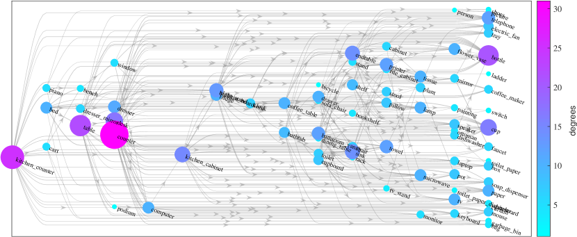
Figure 2: The above graph is generated by the modified IC algorithm on SUNRGBD-3D Dataset. An arrowhead of an edge indicates the direction of causation and the color of a node indicates its degree.

• object category $A$ is found to support object category $B$ (i.e. their relative poses and shapes are such that, within a threshold, one is above and touching the other), or,

• object category $B$ is enclosed/covered by another larger object category $A$ (again this is determined using a threshold on the objects’ relative shapes and poses).

We accept a hypothesis and establish the causal relationship (by entering a suitable edge into the causal graph) if at least $30\%$ of the co-occurrences of these object categories in the dataset agree with the hypothesis. The final directed causal relational graph $\mathcal{G}$ is the union of the causal graphs generated by the above tests. Note that we do not consider any dependencies that would lead to a cycle in the graph [4]. The result of the procedure is also displayed in Figure 2.

3.2 Creating a CFG from the causal graph

We now need to create a Context Free Grammar from the causal graph. The CFG is characterised by non-terminal symbols that generate other symbols. Suppose we choose a particular node in the causal graph (i.e. an object category) and assume it is non-terminal. By tracing the full set of directed edges in the causal graph emanating from this node we create a set of production rules. This non-terminal and associated rules are then tested against the dataset to determine how many scenes are explained (formally “covered”) by the rules. A good choice of non-terminals will lead to good coverage. Our task then is to determine an optimal set of non-terminals and associated rules to give the best coverage of the full dataset of scenes.

Note that finding such a set is a combinatorial hard problem. Therefore, we devise a greedy algorithm to select non-terminals and find approximate best coverage. Let $X_{j}$, an object category, be a potential non-terminal symbol and $\mathcal{R}_{j}$ be the set of production rules derived from $X_{j}$ in the causal graph. Let $C_{j}$ be the set of terminals that $\mathcal{R}_{j}$ covers (essentially nodes that $X_{j}$ leads to in $\mathcal{G}$). Our greedy algorithm begins with an empty set $\mathcal{R}=\emptyset$ and chooses the node $X_{j}$ and associated production rule set $\mathcal{R}_{j}$ to add that maximize the gain in coverage $\mathcal{G}_{gain}(\mathcal{R}_{j},\mathcal{R})=\frac{1}{|\mathcal{R}_{j}|}\sum_{I_{i}\in\mathcal{I}\setminus\mathcal{C}}|Y_{i}|/|I_{i}|$.

Unique parsing Given a scene there could be multiple parse trees derived by the leftmost derivation grammar and hence produces different sequences and different representations. For example, for a scene consist of bed, sofa and pillow, the terminal object pillow could be generated by any of the non-terminals BED or SOFA. This ambiguity can confuse the parser while encoding a scene. Further, different orderings of multiple occurrences of an object lead to different parse trees. We consider following parsing rules to remove the ambiguity:

• Fix the order of the object categories in the order of precedence defined by the grammar.

• Multiple occurrences of an object are sorted in the appearance w.r.t. the preceded object in the anti-clockwise direction starting from the object making minimum angle to the orientation of the preceded object. One such example is shown in Figure 3. Note that this ordering is only required during training.

(a) Ground-truth 1	(b) Ground-truth 2	(c) Ground-truth 3	(d) Ground-truth 4

Figure 3: The parsing order is displayed by a numeral concatenated with the object name. (a) the objects are sorted in the order of precedence defined by the grammar, and (b) multiple chairs are sorted in the appearance w.r.t. the table in anti-clockwise direction starting from the bottom right corner. (c)-(d) More examples of the object order in the ground-truth samples from SUN RGB-D dataset [26].

4 Experiments

Dataset We evaluate the proposed method on SUN RGB-D Dataset [26] consisting of ${10,335}$ real scenes with ${64,595}$ 3D bounding boxes and about $800$ object categories. The dataset is a collection of multiple datasets [10, 25, 32], and is highly unbalanced: e.g. a single object category chair corresponds to about $31\%$ of all the bounding boxes and $38\%$ of total object categories occur just once in the entire dataset. We consider object categories appearing at least $10$ times in the dataset for evaluation. Further, very similar object categories are merged, yielding $84$ object categories and ${62,485}$ bounding boxes.

Table 1: Results of 3D bounding box reconstruction of some of the frequent objects under a valid reconstruction with IoU $>0.25$ [21]. The pose estimation results are furnished within braces (angular errors in degrees, displacement errors in meters).

Objects	chair			bed			table			ktchn$\_$cntr			piano
SG-VAE	$\bm{92.3}$	$({\bf 5.88^{\circ}}{,}$	$\bm{0.13m})$	$\bm{100.0}$	$(\bm{2.80^{\circ}},$	$\bm{0.08m})$	${\bf 96.2}$	$({\bf 2.84^{\circ}},$	$\bm{0.08m})$	${\bf 100.0}$	$(\bm{1.69^{\circ}},$	$\bm{0.08m})$	${\bf 67.1}$	$({\bf 6.93^{\circ}},$	$\bm{0.11m})$
BL1	${75.4}$	${(8.30^{\circ}},$	$\bm{0.14m})$	$98.5$	${(5.70^{\circ}},$	$\bm{0.09m})$	$93.8$	${(3.70^{\circ}},$	$\bm{0.08m})$	$\bm{100.0}$	$({\bf 1.62^{\circ}},$	$\bm{0.06m})$	$48.7$	${(10.3^{\circ}},$	$\bm{0.12m})$
BL2 [6]	$33.7$	${(28.1^{\circ}},$	${0.32m)}$	$75.1$	${(7.12^{\circ}},$	${0.45m)}$	${90.2}$	${(7.69^{\circ}},$	${0.33m)}$	$83.2$	${(5.96^{\circ}},$	${0.09m)}$	$0.80$	${(45.1^{\circ}},$	${0.43m)}$
BL3[14]+[34]	$29.2$	${(41.8^{\circ}},$	${0.26m)}$	$88.7$	${(35.7^{\circ}},$	${0.58m)}$	$72.9$	${(56.7^{\circ}},$	${0.34m)}$	${100.0}$	${(52.5^{\circ}},$	${0.78m)}$	$26.3$	${(17.4^{\circ}},$	${0.33m)}$

We separated $10\%$ of the data at random for validation. On average there are $4.29$ objects per image and maximum number of objects in an image is considered to be $15$. This also provides the upper bound of the length of the sequence generated by the grammar. Note that the dataset is the intersection of the given dataset and the scene language, i.e. the possible set of scenes generated by the CFG.

Table 2: IoU of room layout estimation

Methods	SG-VAE	BL1	BL2 [6]	BL3 [14]+[34]
Grammar	✓	✓		✓
Pose $\&$ Shape	✓	✓	✓
IoU	$\bm{0.6240}$	$0.5673$	$0.2964$	$0.5119$

Baseline methods for evaluation (ablation studies) To evaluate the individual effects of (i) output of the decoder structure, (ii) usage of grammar, and (iii) the pose and shape attributes, the following baselines are chosen:

1. Variant of SG-VAE: In contrast to the proposed SG-VAE where attributes of each rule are directly concatenated with 1-hot encoding of the rule, in this variant separate attributes for each rule type are predicted by the decoder and rest are filled with zeros.

2. No Grammar VAE [6]: No grammar is considered in this baseline. The 1-hot encodings correspond to the object type is concatenated with the absolute pose of the objects (in contrast to rule-type and relative pose in SG-VAE) respectively.

3. Grammar VAE [14] + Make home [34]: The Grammar VAE is incorporated with our extracted grammar to sample a set of coherent objects and [34] is used to arrange them. Sampled $10$ times and solution corresponding to best IoU w.r.t. groundtruth is employed. The details of the above baselines are provided in the supplementary.

All the baselines including SG-VAE are implemented in python 2.7 (Tensorflow) and trained on a GTX 1080 Ti GPU.  
Evaluation metrics The relative poses of individual objects in a scene are accumulated to compute their absolute poses which are then combined with the shape parameters to compute the scene layout. The reconstructed scene layouts are then compared against the groundtruth layouts.

• 3D bounding box reconstruction We employed IoU to measure the shape similarity of the bounding boxes. Reconstructed bounding boxes with IoU $>0.25$ are considered as true positives. The results are reported in Table 1.

• 3D Pose estimation The average pose error is considered over two separate metrices: (i) angular error in degrees, (ii) displacement error in meters (see Table 1).

• Room Layout Estimation The evaluation is conducted as the IoU of the occupied space between the groundtruth and the predicted layouts (see Table 2). The intersection is computed only over the true positives.

	Interpolation 1	Interpolation 2	Interpolation 3	Interpolation 4	Interpolation 5	Interpolation 6

Figure 4: Synthetic scenes decoded from linear interpolations $\alpha\bm{\mu_{1}}+(1-\alpha)\bm{\mu_{2}}$ of the means $\bm{\mu_{1}}$ and $\bm{\mu_{2}}$ of the latent distributions of two separate scenes. The generated scenes are valid in terms of the co-occurrences of the object categories and their shapes and poses (more examples can be found in the supplementary). The room-size and the camera view-point are fixed for better visualization. Best viewed electronically.

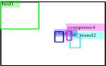
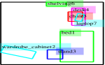
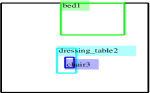
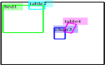
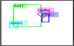
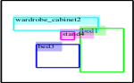
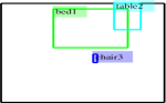
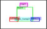
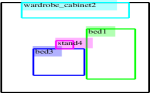
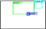
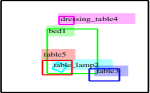
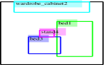
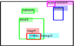
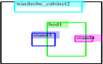
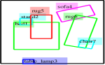
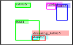
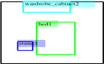
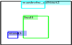
	Interpolation 1	Interpolation 2	Interpolation 3	Interpolation 4	Interpolation 5

Figure 10: Latent code interpolation on SUNCG: Synthetic scenes decoded from linear interpolations $\alpha\bm{\mu_{1}}+(1-\alpha)\bm{\mu_{2}}$ of the means $\bm{\mu_{1}}$ and $\bm{\mu_{2}}$ of the latent distributions of two separate scenes. The generated scenes are valid in terms of the co-occurrences of the object categories and their shapes and poses. The room-size and the camera view-point are fixed for better visualization. Best viewed electronically.

Interpolation in latent space Two distinct scenes are encoded into the latent space, e.g.., $\mathcal{N}(\bm{\mu_{1}},\bm{\Sigma_{1}})$ and $\mathcal{N}(\bm{\mu_{2}},\bm{\Sigma_{2}})$ and new scenes are then synthesized from interpolated vectors of the means, i.e. from $\alpha\bm{\mu_{1}}+(1-\alpha)\bm{\mu_{2}}$. We performed the experiment on a set of random pairs chosen from the test dataset. The results are shown in Figure 10. Notice that the decoder behaves gracefully w.r.t. perturbations of the latent code and always yields a valid and realistic scene.

Figure 5: Top-views of the synthesized scenes generated by the SG-VAE on SUN RGB-D. A detailed comparison with other baselines on SUNCG can be found in supplementary.

4.1 Comparison with baselines on other datasets

The conventional indoor scene synthesis methods (for example, Grains [16], Human-centric [23] (HC), fast-synth [24](FS) etc.) are tailored to and trained on SUNCG dataset [28]. The dataset consists of synthetic scenes generated by graphic designers. Moreover, the dataset is no longer publicly available (along with the meta-files). Therefore the following evaluation protocols are employed to assess the performance of different methods.

Comparison on synthetic scene quality To conduct a qualitative evaluation, we employ a classifier (based on Pointnet [22]) to predict a scene layout to be an original or generated by a scene synthesis method. If the generated scenes are very similar to the original scenes, the classifier performs poorly (lower accuracy) and indicates the efficacy of the synthesis method. The classifier takes a scene layout of multiple objects, individually represented by the concatenation of 1-hot code and the attributes, as input and predicts a binary label according to the scene-type. The classifier is trained and tested on a dataset of $2K$ original and synthetic scenes ($50\%$ training and $50\%$ testing). Note that SG-VAE is trained on the synthetic data generated by the interpolations of latent vectors (some examples are shown in Figure 10) and real data of SUN RGB-D [26]. Lower accuracy of the classifier validates the superior performance of the proposed SG-VAE. The average performance is plotted in Table 3. Examples of some synthetic scenes generated by SG-VAE are also shown in Figure 8.

Table 3: Original vs. synthetic classification accuracy (trained with Pointnet [22]): The accuracy indicates that the synthetic scenes are indistinguishable from the original scenes and hence lower (closer to $50\%$) is better.

Datasets	SUN RGB-D [26]	SUNCG [28]
Methods	SG-VAE	SG-VAE	Grains [16]	HC [23]
Accuracy	$\bm{71.3\%}$	$\bm{83.7\%}$	$96.4\%$	$98.1\%$

Runtime comparison All the methods are evaluated on a single CPU and the runtime is displayed in Table 4. Note that the decoder of the proposed SG-VAE takes only $\sim 1$ms to generate the parse tree and the rest of the time is consumed by the renderer (generating bounding boxes). The proposed method is almost two orders of magnitude faster than the other scene synthesis methods.

Table 4: Average time required to generate a single scene.

Methods	SG-VAE	Grains [16]	FS [24]	HC [23]
Avg. runtime	$\bm{8.5ms}$	$1.2\times 10^{2}ms$	$1.8\times 10^{3}ms$	$2.4\times 10^{5}ms$

4.2 Scene layout estimation from the RGB-D image

The task is to predict the 3D scene layout given an RGB-D image. Typically, the state of the art methods are based on sophisticated region proposals and subsequent processing [27, 21]. With this experiment, we aim to demonstrate the potential use of the latent representation learned by the proposed auto-encoder for a computer vision task, and therefore we employ a simple approach at this point. We (linearly) map deep features (extracted from images by a DNN [38]) to the latent space of the scene-grammar autoencoder. The decoder subsequently generates a 3D scene configuration with associated bounding boxes and object labels from the projected latent vector. Since during the deep feature extraction and the linear projection, the spatial information of the bounding boxes are lost, the predicted scene layout is then combined with a bounding box detection to produce the final output.

(a) Input	(b) SG-VAE	(c) BL1	(d) BL2 [6]	(e)BL3 [14]	(f) DSS [27]	(g) GrndTrth

Figure 6: A few results on SUNRGB Dataset inferred from the RGB-D images.

The bounding box detector of DSS [27] is employed and the scores of the detection are updated based on our reconstruction as follows: the score (confidence of the prediction) of a detected bounding box is doubled if a similar bounding box (in terms of shape and pose) of the same category is reconstructed by our method. A 3D non-maximum suppression is applied to the modified scores to get the final scene layout. The details can be found in the supplementary.

Table 5: IoU for RGBD to room layout estimation

Methods	SG-VAE	BL1	BL2 [6]	BL3 [14]+[34]	DSS [27]
IoU	$\bm{0.4387}$	${0.4315}$	$0.4056$	$0.4259$	$0.4070$

We selected the average IoU for room layout estimation as the evaluation metric, and the results are presented in Table 5. The proposed method and other grammar-based baselines improve the scene layout estimation from the same by sophisticated methods such as deep sliding shapes [27]. Furthermore, the proposed method tackles the problem in a much simpler and faster way. Thus, it can be employed to any 3D scene layout estimation method with very little overhead (e.g.  a few $ms$ in addition to $5.6s$ of [27]). Results on some test images where SG-VAE produces better IoUs are displayed in Figure 6.

5 Related Works

The most relevant method to ours is Grains [16]. It requires training separate networks for each of the room-types—bedroom, office, kitchen etc. HC [23] is very slow and takes a few minutes to synthesize a single layout. FS [24] is fast, but still takes a couple of seconds. SceneGraphNet [33] predicts a probability distribution over object types that fits well in a target location given an incomplete layout. A similar graph-based method is proposed in [29] and CNN-based method proposed in [30] . A complete survey of the relavant method can be found in [35]. Note that all these methods are tailored to and trained on the synthetic SUNCG dataset which is currently unavailable.

Koppula et al. [13] propose a graphical model that captures the local visual appearance and co-occurrences of different objects in the scene. They learn the appearance relationships among objects from the visual features that takes an RGB-D image as input and predicts 3D semantic labels of the objects as output. The pair-wise support relationships of the indoor objects are also exploited in [8, 25]. Learning to 3D scene synthesis from annotated RGB-D images is proposed in [11]. In the similar direction, an example-based synthesis of 3D object arrangements is proposed in [5].

Grammar-based models for 3D scene reconstruction have been partially exploited before [36, 37], e.g.  textured probabilistic grammar [15]. Zhao et al. [36] proposed handcoded grammar to its terminal symbols (line segments) and later extended to different functional groups in [37]. Choi et al. [2] proposed a 3D geometric phrase model that estimates a scene layout with multiple object interactions. Note that all the above methods are based on hand-coded production rules, in contrast, the proposed method exploits a self-supervision to yield the production rules of the grammar.

6 Conclusion

We proposed a grammar-based autoencoder SG-VAE for generating natural indoor scene layouts containing multiple objects. By construction the output of SG-VAE always yields a valid configuration (w.r.t. the grammar) of objects, which was also experimentally confirmed. We demonstrated that the obtained latent representation of an SG-VAE has desirable properties such as the ability to interpolate between latent states in a meaningful way. The latent space of SG-VAE can also be easily adapted to computer vision problems (e.g. 3D scene layout estimation from RGB-D images). Nevertheless, we believe that there is potential in leveraging the latent space of SG-VAEs to the other tasks, e.g. fine-tuning the latent space for a consistent layout over multiple cameras which is part of the future work.

7 Selection of the CFG—Algorithm details

We aim to find suitable non-terminals and associated production rules that cover the entire dataset. Note that finding such a set is a combinatorial hard problem. Therefore, we devise a greedy algorithm to select non-terminals and find approximate best coverage. Let $X_{j}$, an object category, be a potential non-terminal symbol and $\mathcal{R}_{j}$ be the set of production rules derived from $X_{j}$ in the causal graph. Let $C_{j}$ be the set of terminals that $\mathcal{R}_{j}$ covers (essentially nodes that $X_{j}$ leads to in the causal graph $\mathcal{G}$). Our greedy algorithm begins with an empty set $\mathcal{R}=\emptyset$ and chooses the node $X_{j}$ and associated production rule set $\mathcal{R}_{j}$ to add that maximize the gain in coverage

$$\mathcal{G}_{gain}(\mathcal{R}_{j},\mathcal{R})=\frac{1}{|\mathcal{R}_{j}|}\sum_{I_{i}\in\mathcal{I}\setminus\mathcal{C}}|Y_{i}|/|I_{i}|$$ (2)

where $\mathcal{C}$ is the set of scenes that are already covered with a predefined fraction $p$ by the set of rules $\mathcal{R}$, i.e.$\mathcal{C}=\{I_{i}\;|\;\frac{|Y_{i}|}{|I_{i}|}>p\}$ where $Y_{i}$ is the set of terminal symbols occurs while parsing a scene $I_{i}$ by $\mathcal{R}$. The algorithm continues till no further nodes and associated rule set contribute a positive gain or until the current rule set covers the entire dataset with probability $p$ (chosen as $0.8$). We name our algorithm as p-cover and is furnished in algorithm 3. Note that only object co-occurrences were utilized and object appearances were not incorporated in the proposed p-cover algorithm.

To ensure the production rules to form a CFG, we select a few vertices (anchor nodes) of the causal graph and associate a number of non-terminals. A valid production rule is “an object category corresponding to an anchor node generates another object category it is adjacent to in $\mathcal{G}$”. Let us consider the set of anchor nodes forms our set of non-terminals $\Sigma$. The set of all possible objects including dummy None is defined as the set of terminal symbols $\mathcal{V}$.

Let $\mathcal{R}_{j}$ be the set of production rules derived from a non-terminal $X_{j}\text{{inc}}$ corresponding to an anchor object $X_{j}$, and $C_{j}$ be the set of terminals that $\mathcal{R}_{j}$ covers (essentially nodes that $X_{j}$ leads to in $\mathcal{G}$). Note that $\mathcal{R}_{j}$ contains mainly four types of production rules as described in [(R1)-(R4)] in the main text. A few examples of such set of production rules are displayed in Figure 11. The above strategy could lead to a large amount of production rules (ideally sum of number of the anchor points and the number of edges $|\mathcal{E}|$ in the causal graph). Note that a large number of production rules increases the problem complexity. Contrarily, an arbitrary selection of few rules leads to a small number of derivable scenes (language of constituent grammar). We propose an algorithm to find a compressed (minimal size) set of rules to cover the entire dataset. Our underlying assumption is that the distribution of objects in the test scenes is very similar to the distribution of the same in the training scenes. Hence, we use the coverage of the training scenes as a proxy for the coverage of testing scenes and derive a probabilistic covering algorithm on the occurrences of objects in the dataset.

An example snippet for the grammar produced using this algorithm on the SUNRGBD dataset [26] is as follows:  
 
S $\rightarrow$ scene SCENE
SCENE $\rightarrow$ bed BED SCENE
BED $\rightarrow$ bed BED
BED $\rightarrow$ lamp BED
Bed $\rightarrow$ sofa SOFA BED
BED $\rightarrow$ pillow PILLOW BED
BED $\rightarrow$ night$\_$stand BED
BED $\rightarrow$ dresser BED
...
BED $\rightarrow$ None     SCENE $\rightarrow$ sofa sofainc SCENE
SOFA $\rightarrow$ sofa SOFA
SOFA $\rightarrow$ pillow PILLOW SOFA
SOFA $\rightarrow$ TOWEL SOFA
SOFA $\rightarrow$ None
...
SCENE $\rightarrow$ None
 
The entire grammar is displayed in Section 11. In the above snippet the non-terminal BED generates another non-terminal SOFA that leads to an additional set of production rules corresponding to SOFA. Note that the grammar is right-recursive and not a regular grammar as some of the rules contain two non-terminals in the right hand side.

Note that in this grammar non-terminal symbol BED generates another non-terminal SOFA which further leads to another set of production rules corresponding to SOFA. The grammar is right-recursive and not a regular grammar as some of the rules contain two non-terminals in the right hand side.

8 Visualization of the latent space

To check the continuity of the latent space, the latent vectors (i.e., the mean $\bm{\mu}$ of the distribution $\mathcal{N}(\bm{\mu},\bm{\Sigma})$) is projected to 2D plane using data visualization algorithm t-SNE [maaten2008visualizing]. In Figure 7, we display $15$ different scenes in the latent space after t-SNE projection. We observe top left and top right regions are kitchen and bathroom scenes respectively. Whereas, top and bottom regions correspond to bedroom and dining room scenes respectively. The middle region mostly corresponds to living room and office scenes. Note that proposed SG-VAE not only considers the object co-occurrences, also considers object attributes (3D pose and shape parameters). For example, two scenes consists of a chair and a table are mapped to two nearby but distinct points.

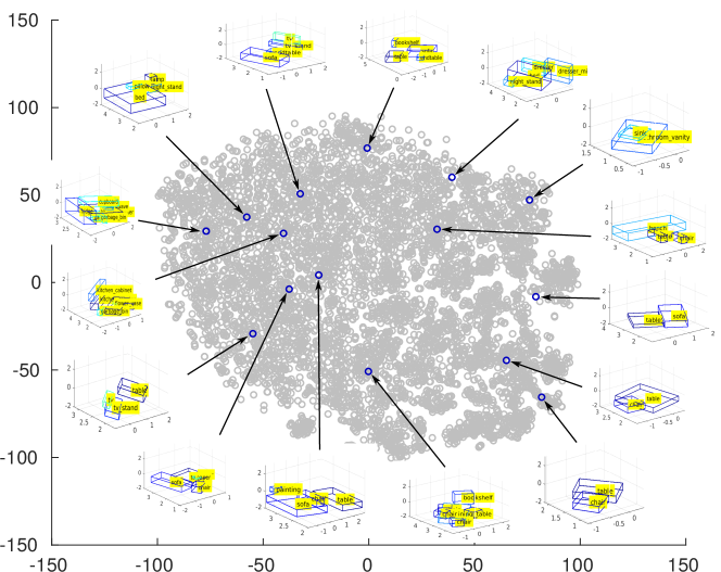
Figure 7: We plot the 2D projection of the mean $\bm{\mu}$ of the encoded distributions of the data (encoded with $50$ dimension) projected using t-SNE algorithm. $15$ chosen scenes are also displayed. Note that points with similar semantic concepts are clustered around a certain region.

9 Results on SUNCG

As mentioned in the paper, due to the ongoing dispute with the SUNCG dataset, we could not include these results in the main paper. The experiment is conducted only on our local copy of the dataset for the reviewing purposes. We extracted $32,765$ bedrooms, $14814$ kitchen, and $8,446$ office rooms from the dataset of $45,622$ synthetic houses. The dataset is divided into $80\%$ training, $10\%$ validation and remaining $10\%$ for testing. The bounding boxes and the relevant parameters are extracted using the scripts provided by Grains .

Baseline comparison For visual comparison, some examples of the scene synthesized by the proposed method along with the baselines on SUNCG are shown in Figure 8. Our results are similar to Grains and better than the other baselines in terms of co-occurrences and appearances (pose and shape) of different objects. A detailed 1-1 comparison with Grains is also shown in Figure 9. The quantitative comparisons are provided in the main manuscript.

Interpolation in the latent space Similar to the interpolation results on SUN RGB-D, shown in the main manuscript, an additional experiment is conducted on SUNCG dataset. Here, synthetic scenes are decoded from linear interpolations $\alpha\bm{\mu_{1}}+(1-\alpha)\bm{\mu_{2}}$ of the means $\bm{\mu_{1}}$ and $\bm{\mu_{2}}$ of the latent distributions of two separate scenes. The generated scenes are valid in terms of the co-occurrences of the object categories and their shapes and poses.

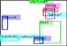
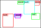
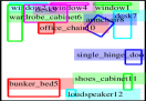
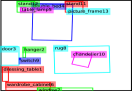
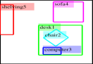
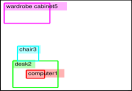
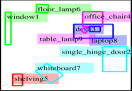
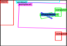
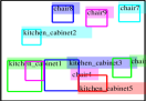
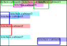
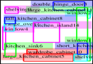
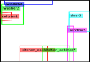
	(a) SG-VAE	(c) Grains [16]	(d) FS [24]	(e) HC [23]

Figure 8: Top-views of the synthesized scenes generated by the proposed and the baseline indoor scene synthesis methods on SUNCG datasets. Note that these are just some random samples taken from the generated scenes.

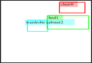
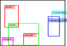
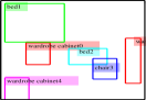
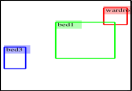
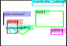
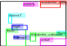
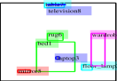
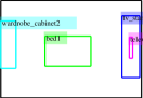
	Sample 1	Sample 2	Sample 3	Sample 4

Figure 9: 1-1 comparison with Grains [16] on SUNCG dataset. Similar samples are chosen for a precise comparison. Most similar synthetic scenes are displayed. We observe that the proposed method SG-VAE produces more variety of objects in a scene than the baseline Grains.

10 Additional experiments on SUN RGBD

10.1 Scene layout from the RGB-D image—in detail

The task is to predict the 3D scene layout given an RGB-D image. We (linearly) map deep features (extracted from images by a DNN [38]) to the latent space of the scene-grammar autoencoder. The decoder subsequently generates a 3D scene configuration with associated bounding boxes and object labels from the projected latent vector. Since during the deep feature extraction and the linear projection, the spatial information of the bounding boxes are lost, the predicted scene layout is then combined with a bounding box detection to produce the final output.

Training Let $\mathcal{F}_{i}$ be the (in our case 8192-dimensional) deep feature vector extracted from the image $I_{i}$, and let $\mathcal{N}(\bm{\mu}_{i},\bm{\Sigma_{i}})$ be the (e.g. 50-dimensional) latent representation obtained by encoding the corresponding parse tree. We align the feature vector $\mathcal{F}_{i}$ with the latent distribution using a linear mapping $\psi(\mathcal{F}_{i})=A\mathcal{F}_{i}$, where $A$ is a matrix to be learned from a training set $\mathcal{T}:=\{I_{i}:=(\mathcal{F}_{i},\bm{\mu}_{i},\bm{\Sigma_{i}})\}$. We minimize the cross-entropy between the predicted (deterministic) latent representation $\psi(\mathcal{F}_{i})$ and the target distribution $\mathcal{N}(\bm{\mu}_{i},\bm{\Sigma_{i}})$, therefore the optimal matrix $A$ is determined as $\hat{A}=\arg\min_{A}\sum_{I_{i}\in\mathcal{T}}\big{(}A\mathcal{F}_{i}-\bm{\mu}_{i}\big{)}^{T}\bm{\Sigma_{i}}^{-1}\big{(}A\mathcal{F}_{i}-\bm{\mu}_{i}\big{)}$ $+\lambda\|A\|_{2}^{2}$. The features $\mathcal{F}_{i}$ of dimension $8192$ are then projected into the mean of the encoded vector $\bm{\mu}_{i}$ (typically dimension $50$). Let $\phi:\mathcal{F}_{i}\rightarrow\bm{\mu}_{i}$ be the mapping that project the feature vectors $\mathcal{F}_{i}$ to the latent space $\bm{\mu}_{i}$. A neural network could be used to learn the mapping $\phi$, however, a simple linear projection is employed here, i.e.$\psi(\mathcal{F}_{i})=A\mathcal{F}_{i}$. The mapping $\phi$ is learned from the training examples $Tr=\{I_{i}:=(\mathcal{F}_{i},\bm{\mu}_{i},\bm{\Sigma_{i}})\}$ as follows:

$$\hat{A} =\arg\min_{A}\sum_{I_{i}\in\mathcal{T}}\Big{(}A\mathcal{F}_{i}-\bm{\mu}_{i}\Big{)}^{T}\bm{\Sigma_{i}}^{-1}\Big{(}A\mathcal{F}_{i}-\bm{\mu}_{i}\Big{)}+\lambda\|A\|_{2}^{2}$$ (3)

where we also added a regularization term with weight $\lambda$ (chosen as $\lambda=100$). Differentiating the objective to zero, we get $\sum_{I_{i}\in\mathcal{T}}\bm{\Sigma_{i}}^{-1}\hat{A}(\mathcal{F}_{i}\mathcal{F}_{i}^{T})+2\lambda\hat{A}$
= $\sum_{I_{i}\in\mathcal{T}}\bm{\Sigma_{i}}^{-1}\bm{\mu}_{i}\mathcal{F}_{i}^{T}$. Therefore,

$$\hat{A} =\Big{(}\sum_{I_{i}\in Tr}\mathcal{F}_{i}^{T}\bm{\Sigma_{i}}^{-1}\mathcal{F}_{i}+2\lambda I\Big{)}^{-1}\sum_{I_{i}\in Tr}\mathcal{F}_{i}\bm{\Sigma_{i}}^{-1}\bm{\mu}_{i}$$ (4)

Note that the covariance matrix $\bm{\Sigma_{i}}$ is chosen to be diagonal, and thus $\hat{A}$ can be solved efficiently. The above is a system of linear equations solved by vectorizing the matrix $\hat{A}$.

Testing For test data image features [38] are extracted and then mapped to the latent space using the trained mapping $\hat{\phi}(\mathcal{F}_{i}):=\mathcal{F}_{i}\hat{A}$. The scenes are then decoded from the latent vectors $\hat{\bm{\mu}}:=\mathcal{F}_{i}\hat{A}$ using the decoder part of the SG-VAE. The bounding box detector of DSS [27] is employed and the scores of the detection are updated based on our reconstruction as follows: the score (confidence of the prediction) of a detected bounding box is doubled if a similar bounding box (in terms of shape and pose) of the same category is reconstructed by our method. A 3D non-maximum suppression is applied to the modified scores to get the final scene layout.

10.2 Quality assessment of the autoencoder

The scenes and the bounding boxes of the test examples are first encoded to the latent representations $\mathcal{N}(\bm{\mu}_{i},\bm{\Sigma_{i}})$. The mean of the distributions $\bm{\mu}_{i}$ are then decoded to the scene with object bounding boxes and labels. The results are displayed below. Ideally, the decoder should produce a scene which is very similar to input test scene. IoU (computed over the occupied space) of the decoded scene and the original input scene is also shown in the main paper. Baseline methods for evaluation as follows:

1. Variant of SG-VAE: In contrast to the proposed SG-VAE where attributes of each rule are directly concatenated with 1-hot encoding of the rule, in this variant separate attributes for each rule type are predicted by the decoder and rest are filled with zeros. i.e., the 1-hot encoding of the production rules is same as SG-VAE but the attributes are represented by a $|\mathcal{R}|*\theta$ dimensional vector where $|\mathcal{R}|$ is the number of production rules and $\theta$ is the size of the attributes. For example, the pose and shape attributes $\Theta^{j\rightarrow k}=({\mathcal{P}}_{i}^{j\rightarrow k},\mathcal{S}_{i}^{k})$, associated with a production rule (say $p$th rule) in which a non-terminal $X_{j}$ yields a terminal $X_{k}$, are placed in $(p-1)*\theta+1:p*\theta$ dimensions of the attribute vector and rest of the positions are kept as zeros. Note that in case of SG-VAE the attributes are represented by a $\theta$ dimensional vector only.

2. No Grammar VAE [6]: No grammar is considered in this baseline. The 1-hot encodings correspond to the object type is concatenated with the absolute pose of the objects (in contrast to rule-type and relative pose in SG-VAE) respectively. i.e.each object is represented by $|\mathcal{V}|$ dimensional 1-hot vector and a $\theta$ dimensional attribute vector. The objects are ordered in the same way as SG-VAE to avoid ambiguity in the representation. The same network as SG-VAE is incorporated except no grammar is employed (i.e.no masking) while decoding a latent vector to a scene layout.

3. Grammar VAE [14] + Make home [34]: The Grammar VAE is incorporated with our extracted grammar to sample a set of coherent objects and [34] is used to arrange them. Sampled $10$ times and solution corresponding to best IoU w.r.t. groundtruth is employed. Here no pose and shape attributes are incorporated while training the autoencoder. The attributes are estimated by Make home [34] and the best (in terms of IoU) is chosen comparing the ground-truth.

The detailed quantitative numbers are presented in the main manuscript.

Input: a dataset $\mathcal{D}$ of natural scenes formed by a set of objects $\mathcal{V}=\{X_{1},\ldots,X_{n}\}$

Output: a graph $\mathcal{G}=\{\mathcal{V},\mathcal{E}\}$ representing the causal relationships between the variables

Initialize $\mathcal{G}:=\{\mathcal{V};\;\mathcal{E}=\mathcal{E}_{0}\}$ ;

  /* Initialize with prior edges */

1 for every pair of objects $(X_{j}\in\mathcal{V};\;X_{j^{\prime}}\in\mathcal{V})$  do

2       for every conditioning variable $X_{k}\in\mathcal{V}\setminus\{X_{i},X_{j^{\prime}}\}$ do

             hypothesis test $X_{j}\raisebox{0.45003pt}{\rotatebox[origin={c}]{90.0}{$\models$}}X_{j^{\prime}}\;|\;X_{k}$ in $\mathcal{D}$ ;

              /* Using Conditional Algo 1 */

3            

4      if no independence was found then

5             add an undirected edge $(X_{j},X_{j}^{\prime})$ in $\mathcal{E}$, i.e., $\mathcal{E}=\mathcal{E}\cup(X_{j},X_{j}^{\prime})$.

6for every pair of objects $(X_{j}\in\mathcal{V};\;X_{j^{\prime}}\in\mathcal{V})$ with a common neighbor $X_{k}$ do

7       if $(X_{j},X_{j}^{\prime})\notin\mathcal{E}$ then

8             if one of $(X_{k},X_{j})$ and $(X_{k},X_{j}^{\prime})$ is directed and the other is undirected or

9             both are undirected then

10                   turn the triplet into a common parent structure, i.e., $X_{j}\hbox{$\leftarrow$}\kern-1.5pt\hbox{$\circ$}X_{k}\hbox{$\circ$}\kern-1.5pt\hbox{$\rightarrow$}X_{j^{\prime}}$

Propagate the arrow orientation for all undirected edges (modify the set $\mathcal{E}$ accordingly) without introducing a directed cycle. ;

  /* Following Dor and Tarsi [4] */

return $\mathcal{G}=\{\mathcal{V},\mathcal{E}\}$

Algorithm 2 Structure learning: Inductive Causation (IC) [20]

11 Production rules extracted from SUN RGB-D

Here we describe the production rules of the CFG extracted from SUN RGB-D dataset in detail. The total number of rules generated by the algorithm described in section 3 of the main draft is $399$, number of non-terminals is $49$ and number of terminal objects is $84$. In the following we display the entire learned grammar. Note again that the non-terminal symbols are displayed in upper case, S is the start symbol and None is the empty object. The rules are separated by semicolons ‘ ; ’ symbol.

Input: a dataset $\mathcal{D}$ of indoor scenes $\mathcal{I}$ formed by a set of objects $\mathcal{V}=\{X_{1},\ldots,X_{n}\}$, the causal graph $\mathcal{G}=(\mathcal{V},\mathcal{E})$ obtained by Algorithm 2 and a probability $p$ (chosen as $0.8$)

Output: a set of rules $\mathcal{R}$ that explains the occurrences of objects in the scenes $\mathcal{I}$

Choose the set of potential non-terminals as $\mathcal{V}^{\prime}=\{X_{i}\in\mathcal{V}:deg_{out}(X_{i})/(deg_{in}(X_{i})+\epsilon)>1\}$ ;

  /* Proportion of the outward degree and inward degree; $\epsilon<1$ */

Generate set of concepts and associated rules $\{\mathcal{R}_{j}\}_{j\in\mathcal{V}^{\prime}}$ by choosing adjacent objects ;

  /* Some examples are displayed in Figure 11 */

Initialize $\mathcal{R}\leftarrow\emptyset$, $\mathcal{V}^{\star}=\emptyset$, and $C=\emptyset$ ;

  /* Initialize by empty set; */

1 while the cover set $\mathcal{C}$ covers the dataset with probability $p$ do

2       for every non-terminal and associated set of rules $\mathcal{R}_{j}$, $\forall j\in\mathcal{V}^{\prime}\setminus\mathcal{V}^{\star}$ do

3             Compute the gain $\mathcal{G}_{gain}(\mathcal{R}_{j},\mathcal{R})$ as referred in Eq. 2 of the main draft

4      compute next anchor node $X_{\bar{j}}=\operatorname*{arg\,max}_{X_{j}\in\mathcal{V}^{\prime}\setminus\mathcal{V}^{\star}}\mathcal{G}_{gain}(\mathcal{R}_{j},\mathcal{R})$ and $\mathcal{V}^{\star}=\mathcal{V}^{\star}\cup{\bar{X_{j}}}$

5       $\mathcal{R}=\mathcal{R}\cup\mathcal{R}_{\bar{j}}$

       $C=C\cup C_{\bar{j}}$ ;

        /* Update the rule set and the cover set; */

6      

7$\mathcal{R}=\mathcal{R}\cup[S\rightarrow\text{{'None'}}]$

return $\mathcal{R}$

Algorithm 3 p-Cover : A greedy algorithm for p-cover

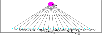
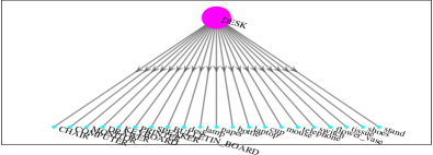
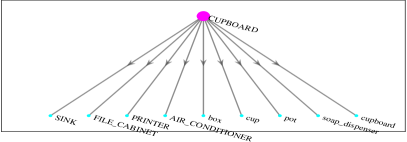
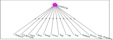
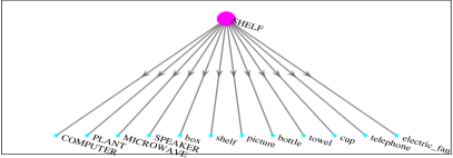
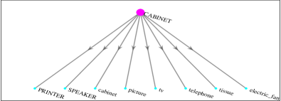
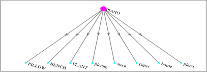
Figure 11: A few examples of the production rule-sets $R_{j}$ which are utilized to generate the CFG. The detail algorithm is furnished in algorithm 3. The non-terminal symbols are displayed in upper-case and terminal symbols are shown in lower-case.

References

- [1] Anderson, P., He, X., Buehler, C., Teney, D., Johnson, M., Gould, S., Zhang, L.: Bottom-up and top-down attention for image captioning and visual question answering. In: Proceedings of CVPR. pp. 6077–6086 (2018)
- [2] Choi, W., Chao, Y.W., Pantofaru, C., Savarese, S.: Understanding indoor scenes using 3d geometric phrases. In: Proceedings of CVPR. pp. 33–40 (2013)
- [3] Deng, C., Wu, Q., Wu, Q., Hu, F., Lyu, F., Tan, M.: Visual grounding via accumulated attention. In: Proceedings of CVPR. pp. 7746–7755 (2018)
- [4] Dor, D., Tarsi, M.: A simple algorithm to construct a consistent extension of a partially oriented graph (1992)
- [5] Fisher, M., Ritchie, D., Savva, M., Funkhouser, T., Hanrahan, P.: Example-based synthesis of 3d object arrangements. ACM Transactions on Graphics (TOG) 31(6), 1–11 (2012)
- [6] Gómez-Bombarelli, R., Wei, J.N., Duvenaud, D., Hernández-Lobato, J.M., Sánchez-Lengeling, B., Sheberla, D., Aguilera-Iparraguirre, J., Hirzel, T.D., Adams, R.P., Aspuru-Guzik, A.: Automatic chemical design using a data-driven continuous representation of molecules. ACS central science 4(2), 268–276 (2018)
- [7] Goodfellow, I., Pouget-Abadie, J., Mirza, M., Xu, B., Warde-Farley, D., Ozair, S., Courville, A., Bengio, Y.: Generative adversarial nets. In: Proceedings of NIPS. pp. 2672–2680 (2014)
- [8] Guo, R., Hoiem, D.: Support surface prediction in indoor scenes. In: Proceedings of ICCV. pp. 2144–2151 (2013)
- [9] Huang, S., Qi, S., Zhu, Y., Xiao, Y., Xu, Y., Zhu, S.C.: Holistic 3d scene parsing and reconstruction from a single rgb image. In: Proceedings of ECCV. pp. 187–203 (2018)
- [10] Janoch, A., Karayev, S., Jia, Y., Barron, J.T., Fritz, M., Saenko, K., Darrell, T.: A category-level 3d object dataset: Putting the kinect to work. In: Consumer depth cameras for computer vision, pp. 141–165. Springer (2013)
- [11] Kermani, Z.S., Liao, Z., Tan, P., Zhang, H.: Learning 3d scene synthesis from annotated rgb-d images. In: Computer Graphics Forum. vol. 35, pp. 197–206. Wiley Online Library (2016)
- [12] Kingma, D.P., Welling, M.: Auto-encoding variational bayes. In: Proceedings of ICLR. pp. 469–477 (2014)
- [13] Koppula, H.S., Anand, A., Joachims, T., Saxena, A.: Semantic labeling of 3d point clouds for indoor scenes. In: Proceedings of NIPS. pp. 244–252 (2011)
- [14] Kusner, M.J., Paige, B., Hernández-Lobato, J.M.: Grammar variational autoencoder. In: Proceedings of ICML. pp. 1945–1954. JMLR. org (2017)
- [15] Li, D., Hu, D., Sun, Y., Hu, Y.: 3d scene reconstruction using a texture probabilistic grammar. Multimedia Tools and Applications 77(21), 28417–28440 (2018)
- [16] Li, M., Patil, A.G., Xu, K., Chaudhuri, S., Khan, O., Shamir, A., Tu, C., Chen, B., Cohen-Or, D., Zhang, H.: Grains: Generative recursive autoencoders for indoor scenes. ACM Transactions on Graphics (TOG) 38(2), 12 (2019)
- [17] Liu, M.Y., Tuzel, O.: Coupled generative adversarial networks. In: Proceedings of NIPS. pp. 469–477 (2016)
- [18] Lu, J., Yang, J., Batra, D., Parikh, D.: Hierarchical question-image co-attention for visual question answering. In: Proceedings of NIPS. pp. 289–297 (2016)
- [19] Meyer, J.A., Filliat, D.: Map-based navigation in mobile robots:: Ii. a review of map-learning and path-planning strategies. Cognitive Systems Research 4(4), 283–317 (2003)
- [20] Pearl, J., Verma, T.S.: A theory of inferred causation. In: Studies in Logic and the Foundations of Mathematics, vol. 134, pp. 789–811. Elsevier (1995)
- [21] Qi, C.R., Chen, X., Litany, O., Guibas, L.J.: Imvotenet: Boosting 3d object detection in point clouds with image votes. In: Proceedings of CVPR. pp. 4404–4413 (2020)
- [22] Qi, C.R., Su, H., Mo, K., Guibas, L.J.: Pointnet: Deep learning on point sets for 3d classification and segmentation. In: Proceedings of CVPR. pp. 652–660 (2017)
- [23] Qi, S., Zhu, Y., Huang, S., Jiang, C., Zhu, S.C.: Human-centric indoor scene synthesis using stochastic grammar. In: Proceedings of CVPR. pp. 5899–5908 (2018)
- [24] Ritchie, D., Wang, K., Lin, Y.a.: Fast and flexible indoor scene synthesis via deep convolutional generative models. In: Proceedings of CVPR. pp. 6182–6190 (2019)
- [25] Silberman, N., Hoiem, D., Kohli, P., Fergus, R.: Indoor segmentation and support inference from rgbd images. In: Proceedings of ECCV. pp. 746–760. Springer (2012)
- [26] Song, S., Lichtenberg, S.P., Xiao, J.: Sun rgb-d: A rgb-d scene understanding benchmark suite. In: Proceedings of CVPR. pp. 567–576 (2015)
- [27] Song, S., Xiao, J.: Deep sliding shapes for amodal 3d object detection in rgb-d images. In: Proceedings of CVPR. pp. 808–816 (2016)
- [28] Song, S., Yu, F., Zeng, A., Chang, A.X., Savva, M., Funkhouser, T.: Semantic scene completion from a single depth image. In: Proceedings of CVPR. pp. 1746–1754 (2017)
- [29] Wang, K., Lin, Y.A., Weissmann, B., Savva, M., Chang, A.X., Ritchie, D.: Planit: Planning and instantiating indoor scenes with relation graph and spatial prior networks. ACM Transactions on Graphics (TOG) 38(4), 1–15 (2019)
- [30] Wang, K., Savva, M., Chang, A.X., Ritchie, D.: Deep convolutional priors for indoor scene synthesis. ACM Transactions on Graphics (TOG) 37(4), 1–14 (2018)
- [31] Xiao, F., Sigal, L., Jae Lee, Y.: Weakly-supervised visual grounding of phrases with linguistic structures. In: Proceedings of CVPR. pp. 5945–5954 (2017)
- [32] Xiao, J., Owens, A., Torralba, A.: Sun3d: A database of big spaces reconstructed using sfm and object labels. In: Proceedings of ICCV. pp. 1625–1632 (2013)
- [33] Yang Zhou, Zachary While, E.K.: Scenegraphnet: Neural message passing for 3d indoor scene augmentation. In: Proceedings of ICCV (2019)
- [34] Yu, L.F., Yeung, S.K., Tang, C.K., Terzopoulos, D., Chan, T.F., Osher, S.J.: Make it home: automatic optimization of furniture arrangement. In: ACM Transactions on Graphics (TOG). vol. 30, p. 86. ACM (2011)
- [35] Zhang, S.H., Zhang, S.K., Liang, Y., Hall, P.: A survey of 3d indoor scene synthesis. Journal of Computer Science and Technology 34(3), 594–608 (2019)
- [36] Zhao, Y., Zhu, S.C.: Image parsing with stochastic scene grammar. In: Proceedings of NIPS. pp. 73–81 (2011)
- [37] Zhao, Y., Zhu, S.C.: Scene parsing by integrating function, geometry and appearance models. In: Proceedings of CVPR. pp. 3119–3126 (2013)
- [38] Zhou, B., Lapedriza, A., Xiao, J., Torralba, A., Oliva, A.: Learning deep features for scene recognition using places database. In: Proceedings of NIPS. pp. 487–495 (2014)