Formation of the Hayward black hole from a collapsing shell

Abstract

We consider a collapsing shell of matter to form the Hayward black hole and investigate semi-classically quantum radiation from the shell. Using the Israel’s formulation, we obtain the mass relation between the collapsing shell and the Hayward black hole. By using the functional Schrödinger formulation for the massless quantum radiation, the evolution of a vacuum state for a scalar field is shown to be unitary. We find that the number of quanta at a low frequency decreases for a large length parameter characterizing the Hayward black hole. Moreover, in the limit of low frequency, the Hawking temperature can be read off from the occupation number of excited states when the shell approaches its own horizon.

I introduction

Since physical singularities of black holes have been interpreted as a breakdown of general relativity, there has been much attention to singularity-free black holes, the so-called regular black holes Bardeen:1968 ; Borde:1996df ; AyonBeato:1999ec ; Hayward:2005gi ; Bambi:2013ufa ; Balart:2014cga . Among these black hole solutions, in particular, the metric of the Hayward black hole reduces to the geometry of Schwarzschild black hole for a large radius, and to the metric of the de Sitter spacetime for a small radius so that the curvature becomes nonsingular at the center Hayward:2005gi . In the Hayward black hole, various aspects have been also studied in Refs. Halilsoy:2013iza ; Abbas:2014oua ; Amir:2015pja ; Pourhassan:2016qoz ; Chiba:2017nml ; Mehdipour:2016vxh .

On the other hand, the functional Schrödinger picture was formulated in order for studying quantum radiation from a collapsing shell Vachaspati:2006ki ; Vachaspati:2007hr . The process of the collapsing shell to form the Schwarzschild black hole was constructed, so massless quantum radiation as seen by an observer at asymptotic infinity turned out to be nonthermal. Subsequently, there have been several works employing this method such as studies on radiation as seen by an infalling observer Greenwood:2008zg , collapsing shells to form the Bañados-Teitelboim-Zanelli black string Greenwood:2009gp , Hawking radiation from the Reissner-Nordström domain wall Greenwood:2009pd , and a massive quantum radiation Greenwood:2010sx . In addition, thanks to an analytic solution of the functional Schödinger equation in Ref. Kolopanis:2013sty , the density matrix of the quantum radiation was also calculated explicitly, which shows that the process of the radiation is unitary during the evolution Saini:2015dea ; Saini:2016rrt . This fact was confirmed in the other singular black holes such as the anti-de Sitter Schwarzschild black hole and the Reissner-Nordström black hole Saini:2017mur ; Das:2019iru . Now, one might wonder how this collapsing process including the functional Schrodinger method works in the Hayward black hole as a regular black hole.

In this paper, we will study the process of a collapsing shell to form the Hayward black hole and investigate the quantum radiation in the context of the functional Schrödinger equation. In Sec. II, we will obtain a mass relation between the collapsing shell and the Hayward black hole by using the Israel formulation Israel:1966rt . Next, in Sec. III, a massless quantum radiation from the shell will be studied by using the functional Schrödinger equation for two cases: when the shell forms the nonextremal black hole and when the horizon is absent. In the former case, the analytic solution of the functional Schrödinger equation will be obtained in the Hayward black hole along the line of Refs. Vachaspati:2006ki ; Kolopanis:2013sty , and eventually, the process is shown to be unitary. In the latter case, we will take the limit of a small radius for the final stage of the collapsing shell, and thus, the analytic solution will also be obtained. In Sec. IV, in the two cases in Sec. III, we will calculate the occupation number of excited states and discuss the spectrum of the occupation number. In the former case, the occupation number at a low frequency will be shown to decrease for a larger value of $\ell$ being a length parameter in the Hayward black hole. In the latter case, the spectrum of the occupation number will turn out to be damped oscillating for the final stage of the collapsing. Finally, a conclusion and discussion will be given in Sec. V.

II classical theory for a collapsing shell to form the Hayward black hole

The spacetime will be divided into the interior and the exterior regions of an infinitely thin shell with a radius $R(t)$ Vachaspati:2006ki ; Vachaspati:2007hr ; Greenwood:2008zg ; Greenwood:2009gp ; Greenwood:2009pd ; Greenwood:2010sx ; Saini:2015dea ; Saini:2016rrt ; Saini:2017mur ; Das:2019iru . In the exterior region of the shell, i.e., $r>R(t)$, the spacetime is described by the Hayward metric Hayward:2005gi ,

$$\left(ds_{+}\right)^{2}=-f(r)dt^{2}+\frac{1}{f(r)}dr^{2}+r^{2}d\Omega^{2}$$ (1)

with $f(r)=1-2Mr^{2}/(r^{3}+2\ell^{2}M)$, where $M$ is the mass of the Hayward black hole and $\ell$ is the length parameter related to cosmological constant as $\Lambda=3/\ell^{2}$. The metric (1) reduces to the Schwarzschild metric for $\ell=0$, and it becomes Minkowski spacetime for $M=0$. Note that there is a critical mass $M^{*}=3\sqrt{3}\ell/4$ to form a black hole such that $\ell_{\max}=4M^{*}/(3\sqrt{3})$ Hayward:2005gi ; $f(r)$ has two simple zeros if $M>M^{*}$ ($\ell<\ell_{\max}$), one double zero if $M=M^{*}$ ($\ell=\ell_{\max}$), and no zeros if $M<M^{*}$ ($\ell>\ell_{\max}$). Next, in the interior region of the shell, the spacetime is assumed to be Minkowski spacetime described by the metric,

$$\left(ds_{-}\right)^{2}=-dT^{2}+dr^{2}+r^{2}d\Omega^{2},$$ (2)

which is valid for $r<R(t)$. On the shell $r=R(t)$, the proper distance is required to be continuous as $\left(ds_{+}\right)^{2}|_{r\to R(t)}=\left(ds_{-}\right)^{2}|_{r\to R(t)}$, so a relation between the exterior and interior times is obtained as

$$\frac{dT}{dt}\bigg{|}_{r=R(t)}=\sqrt{f(R)+\left(1-\frac{1}{f(R)}\right)\dot{R}^{2}},$$ (3)

where $\dot{R}=dR/dt$.

In the Israel formulation Israel:1966rt , a combined metric can be obtained as $g_{\mu\nu}=\Theta(r-R(t))\tilde{g}^{+}_{\mu\nu}+\Theta(-r+R(t))\tilde{g}^{-}_{\mu\nu}$, where $\Theta(x)$ is the unit step function defined as $\Theta(x)=1(x>0)$ and $\Theta(x)=0(x<0)$ with the metrics being $\tilde{g}^{+}_{\mu\nu}$ and $\tilde{g}^{-}_{\mu\nu}$ in the exterior and the interior regions, respectively. Then, a junction condition requires that $g_{\mu\nu}$ be continuous on the shell, so the Einstein tensor can be calculated as

$$G_{\mu\nu}=\Theta(r-R(t))\tilde{G}^{+}_{\mu\nu}+\Theta(-r+R(t))\tilde{G}^{-}_{\mu\nu}+\delta(r-R(t))\tilde{G}^{0}_{\mu\nu},$$ (4)

where $\tilde{G}^{\pm}_{\mu\nu}$ and $\tilde{G}^{0}_{\mu\nu}$ are Einstein tensors calculated in the exterior and interior regions, and on the shell. Explicitly, $\tilde{G}^{0}_{\mu\nu}=\left\{\kappa_{\mu\gamma}n^{\gamma}n_{\nu}\!+\!n_{\mu}n^{\gamma}\kappa_{\gamma\nu}\!+\!\kappa_{\gamma}^{\gamma}(g_{\mu\nu}\!-\!n_{\mu}n_{\nu})\!-\!\kappa_{\mu\nu}\!-\!g_{\mu\nu}n^{\gamma}\kappa_{\gamma\delta}n^{\delta}\right\}/2$, where $\kappa_{\mu\nu}=n^{\gamma}\left(\partial_{\gamma}\tilde{g}_{\mu\nu}^{+}|_{r\to R(t)}-\partial_{\gamma}\tilde{g}_{\mu\nu}^{-}|_{r\to R(t)}\right)$ and $n^{\mu}$ is a unit normal vector to the shell. From the Einstein tensor (4), the corresponding energy-momentum tensor can also be calculated as

$$T_{\mu\nu}=\Theta(r-R(t))\tilde{T}^{+}_{\mu\nu}+\Theta(-r+R(t))\tilde{T}^{-}_{\mu\nu}+\delta(r-R(t))\tilde{T}^{0}_{\mu\nu}.$$ (5)

Projecting $\tilde{G}^{0}_{\mu\nu}=8\pi\tilde{T}^{0}_{\mu\nu}$ to the shell by using the projection operator $h_{\mu\nu}=g_{\mu\nu}-n_{\mu}n_{\nu}$, we obtain the so-called Israel relation,

$$\left[Kh_{\mu\nu}\right]-\left[K_{\mu\nu}\right]=8\pi S_{\mu\nu},$$ (6)

where $K_{\mu\nu}$ is the extrinsic curvature of the shell and $[...]$ denotes $[A]=\lim_{r\to R+}A(r)-\lim_{r\to R-}A(r)$. Now, the source on the shell is assumed to be described by a perfect fluid; thus, $S^{\mu\nu}=h_{\mu}^{\gamma}\tilde{T}_{\gamma\nu}^{0}=(\sigma-\tau)u^{\mu}u^{\nu}-\tau h^{\mu\nu}$, where $\sigma$ is an energy density and $\tau$ is a surface tension Israel:1966rt . In particular, a domain wall satisfying the relation $\sigma=\tau$ can be chosen as a source, so the source on the shell reduces to $S^{\mu\nu}=-\sigma h^{\mu\nu}$. Note that the energy density turns out to be constant thanks to the conservation equation on the shell $h_{\mu\gamma}D_{\nu}S^{\gamma\nu}=0$, where $D_{\mu}=h_{\mu}^{\nu}\nabla_{\nu}$ Ipser:1983db ; Lopez:1988gt .

Plugging $S_{\mu\nu}$ into Eq. (6), we finally obtain the mass relation,

$$\frac{f(R)}{\sqrt{f(R)-\frac{\dot{R}^{2}}{f(R)}}}-\frac{1}{\sqrt{1-\frac{\dot{R}^{2}}{B^{2}}}}=-4\pi\sigma R,$$ (7)

with $B^{2}=(dT/dt)^{2}\big{|}_{r=R(t)}$. For a static limit, i.e., ${\dot{R}}=0$, the mass in Eq. (1) can be expressed in terms of the mass $M_{0}=4\pi R^{2}\sigma$ on the shell in such a way that

$$M=\frac{M_{0}-\frac{M_{0}^{2}}{2R}}{1-\frac{2\ell^{2}}{R^{3}}\left(M_{0}-\frac{M_{0}^{2}}{2R}\right)},$$ (8)

which can be reduced to the case of the Schwarzschild black hole as $\ell\to 0$ Vachaspati:2006ki . From Eq. (7) with Eq. (3), a first-order differential equation can be obtained as

$$\frac{dR}{dt}=-\frac{f(R)}{\sqrt{1+f(R)\left[1-\frac{R^{2}}{4M_{0}^{2}}\left(M_{0}^{2}+1-f(R)\right)^{2}\right]^{-1}}}.$$ (9)

In order to study the collapsing shell to form the Hayward black hole, we will investigate the case of $M>M^{*}$. When the collapsing shell starts to form the black hole as $R(t)\to R_{H}$, Eq. (9) reduces to a simple form as Vachaspati:2006ki ; Vachaspati:2007hr ; Greenwood:2008zg ; Greenwood:2009gp ; Greenwood:2009pd ; Greenwood:2010sx ; Saini:2015dea ; Saini:2016rrt ; Saini:2017mur ; Das:2019iru

$$\frac{dR}{dt}\approx-f(R).$$ (10)

Solving this equation in this incipient limit, we get the radius $R(t)=R_{H}+(R_{0}-R_{H})e^{-f^{\prime}(R_{H})t}$ for $0\leq t\leq t_{f}$, while the initial and the final radii are $R_{0}=R(t_{0})$ for $t<0$ and $R_{f}=R(t_{f})$ for $t>t_{f}$, respectively.

In the case of $M<M^{*}$ where the horizon is absent, $(dR/dt)$ is regular, the shell shrinks continuously and then finally reaches $R=0$. Since it would be a highly nontrivial task to solve Eq. (9) analytically in the whole region, we will discuss the limiting case of a small radius ($R\to 0$). As $R\to 0$ in Eq. (9), $(dR/dt)\to-1/\sqrt{2}$ and so,

$$R(t)=R_{0}-\frac{t}{\sqrt{2}},$$ (11)

where $t_{\rm max}=\sqrt{2}R_{0}$ for the positivity of the radius.

III quantum radiation from the collapsing shell

If an observer at asymptotic infinity sees the formation of the black hole, one can ask what radiation that characterizes gravitational collapse might be observed. Hence, we consider a quantum scalar field on the background of the collapsing shell and derive a quantized theory of the scalar field on the Hayward black hole.

The total action for a single scalar field is assumed to consist of both the exterior and the interior actions such as

$$S_{\Phi} = S^{+}_{\Phi}+S^{-}_{\Phi},$$ (12)

$$S^{\pm}_{\Phi} = \int{\textrm{d}}^{4}x_{\pm}\sqrt{-g^{\pm}}\left(-\frac{1}{2}g^{\pm}~{}^{\mu\nu}\partial^{\pm}_{\mu}\Phi\partial^{\pm}_{\nu}\Phi\right),$$ (13)

where $g^{+}_{\mu\nu}$ and $g^{-}_{\mu\nu}$ are the Hayward metric (1) and the Minkowski metric (2), and $x_{\pm}^{\mu}$ are the exterior and the interior coordinates, respectively. By using the spherical symmetries of the metrics, the scalar field can be decomposed into real spherical harmonics as

$$\Phi(x_{\pm}^{0},r,\theta,\phi)=\sum_{j,m_{j}}\Phi_{j}(x_{\pm}^{0},r)Y_{j,m_{j}}(\theta,\phi)$$ (14)

with $j=0,1,2,...$ and $m_{j}=-j,-j+1,...,j$. Then, the actions (13) can be written as

$$S^{+}_{\Phi} =\sum_{j}4\pi(2j+1)\int\!\!{\textrm{d}}t\int_{R}^{\infty}\!\!{\textrm{d}}r\left(\frac{r^{2}}{2f(r)}\left(\frac{\partial\Phi_{j}}{\partial t}\right)^{2}-\frac{r^{2}f(r)}{2}\left(\frac{\partial\Phi_{j}}{\partial r}\right)^{2}-\frac{j(j+1)}{2}\Phi_{j}^{2}\right),$$ (15)

$$S^{-}_{\Phi} =\sum_{j}4\pi(2j+1)\int{\textrm{d}}T\int_{0}^{R}{\textrm{d}}r\left(\frac{r^{2}}{2}\left(\frac{\partial\Phi_{j}}{\partial T}\right)^{2}-\frac{r^{2}}{2}\left(\frac{\partial\Phi_{j}}{\partial r}\right)^{2}-\frac{j(j+1)}{2}\Phi_{j}^{2}\right).$$ (16)

Especially, the interior action (16) is written as

$$S^{-}_{\Phi}=\sum_{j}4\pi(2j+1)\int{\textrm{d}}t\int_{0}^{R}{\textrm{d}}r\left(\frac{r^{2}}{2B}\left(\frac{\partial\Phi_{j}}{\partial t}\right)^{2}-\frac{r^{2}B}{2}\left(\frac{\partial\Phi_{j}}{\partial r}\right)^{2}-\frac{j(j+1)B}{2}\Phi_{j}^{2}\right),$$ (17)

where we have used the relation $B=\left(dT/dt\right)|_{r=R(t)}$ in Eq. (3). In the functional Schrödinger formalism, one can derive the Schrödinger equation by using the Hamiltonian given as the Legendre transformation of the action (12). Since $R(t)$ was calculated analytically for the cases of $M>M^{*}$ and $M<M^{*}$ in the previous section and $B$ in Eq. (17) is a function of $R(t)$, we can study the Hamiltonian analytically in each case. In the following subsections, Secs. III.1 and III.2, we will study the quantum radiation by using the functional Schrödinger formalism for $M>M^{*}$ and $M<M^{*}$.

III.1 Presence of the horizon ($M>M^{*}$)

In order to study a nonextremal black hole, the case of $M>M^{*}$ will be considered. We decompose $\Phi_{j}$ into a complete set of real basis functions denoted by $\{d_{k,j}\}$ Vachaspati:2006ki ,

$$\Phi_{j}=\sum_{k}a_{k,j}(t)d_{k,j}(r),$$ (18)

where $a_{k,j}(t)$ is a mode amplitude. By using Eq. (18), in the incipient limit $R\to R_{H}$, the action (12) is obtained as

$$S_{\Phi}\approx\sum_{k,k^{\prime},j}(2j+1)\int{\textrm{d}}t\left(\frac{1}{2f(R)}\dot{a}_{k,j}\tilde{A}_{k,k^{\prime},j}\dot{a}_{k^{\prime},j}-\frac{1}{2}a_{k,j}(\tilde{B}_{k,k^{\prime},j}+\tilde{C}_{k,k^{\prime},j})a_{k^{\prime},j}\right)$$ (19)

after spatial integrations, where the coefficients are defined by

$$\tilde{A}_{k,k^{\prime},j} =4\pi\int_{0}^{R_{H}}{\textrm{d}}rr^{2}d_{k,j}d_{k^{\prime},j}~{},$$ (20)

$$\tilde{B}_{k,k^{\prime},j} =4\pi\int_{R_{H}}^{\infty}{\textrm{d}}rr^{2}f(r)\frac{{\textrm{d}}d_{k,j}}{{\textrm{d}}r}\frac{{\textrm{d}}d_{k^{\prime},j}}{{\textrm{d}}r}~{},$$ (21)

$$\tilde{C}_{k,k^{\prime},j} =4\pi j(j+1)\int_{R_{H}}^{\infty}{\textrm{d}}rd_{k,j}d_{k^{\prime},j}.$$ (22)

Since the coefficients $\tilde{A}_{k,k^{\prime},j}$, $\tilde{B}_{k,k^{\prime},j}$, and $\tilde{C}_{k,k^{\prime},j}$ are Hermitian operators, they can be simultaneously diagonalized by a set of eigenvectors $\{b_{k,j}\}$ goldstein:mechanics ; Vachaspati:2006ki ,

$$S_{\Phi}=\sum_{k,j}(2j+1)\int{\textrm{d}}t\left(\frac{1}{2f(R)}\alpha_{k,j}\dot{b}_{k,j}^{2}-\frac{1}{2}(\beta_{k,j}+\gamma_{k,j})b_{k,j}^{2}\right),$$ (23)

where $\alpha_{k,j}$, $\beta_{k,j}$, and $\gamma_{k,j}$ are eigenvalues of $\tilde{A}_{k,k^{\prime},j}$, $\tilde{B}_{k,k^{\prime},j}$, and $\tilde{C}_{k,k^{\prime},j}$, respectively.

We are now in a position to impose the quantization rule as $\left[b_{k,j},\Pi_{k^{\prime},j^{\prime}}\right]=i\delta_{k,k^{\prime}}\delta_{j,j^{\prime}}$ represented by $\Pi_{k,j}\to-i\partial/\partial b_{k,j}$, where $\Pi_{k,j}=\partial L_{\Phi}/\partial\dot{b}_{k,j}=(2j+1)\alpha_{k,j}\dot{b}_{k,j}/f(R)$. Hence, the Hamiltonian for the quantum radiation can be obtained as

$$H_{\Phi}=\sum_{k,j}\left(-\frac{f(R)}{2(2j+1)\alpha_{k,j}}\frac{\partial^{2}}{\partial b_{k,j}^{2}}+\frac{1}{2}(\beta_{k,j}+\gamma_{k,j})b_{k,j}^{2}\right).$$ (24)

From the functional Schrödinger equation $H_{\Phi}\Psi=i\partial\Psi/\partial t$ Vachaspati:2006ki , the Schrödinger equation of the wave function $\psi$ for one eigenvector $b\in\{b_{k,j}\}$ can be written as

$$\left\{-\frac{f(R)}{2\alpha}\frac{\partial^{2}}{\partial b^{2}}+\frac{1}{2}\alpha\omega_{0}^{2}b^{2}\right\}\psi(t,b)=i\frac{\partial\psi}{\partial t}(t,b),$$ (25)

where $\omega_{0}=\sqrt{(2j+1)(\beta+\gamma)/\alpha}$ with $\alpha\in\{(2j+1)\alpha_{k,j}\}$, $\beta\in\{\beta_{k,j}\}$, and $\gamma\in\{\gamma_{k,j}\}$. For convenience, a new time parameter is defined as

$$\eta=\int_{0}^{t}\textrm{d}t^{\prime}~{}f(R(t^{\prime}))$$ (26)

so that Eq. (25) becomes the Schrödinger equation for a harmonic oscillator with the mass $\alpha$ and the time-dependent frequency $\omega(\eta)$ as

$$\left[-\frac{1}{2\alpha}\frac{\partial^{2}}{\partial b^{2}}+\frac{1}{2}\alpha\omega^{2}(\eta)b^{2}\right]\psi(\eta,b)=i\frac{\partial\psi}{\partial\eta}(\eta,b),$$ (27)

where $\omega(\eta)=\omega_{0}/\sqrt{f(R)}$. For $\eta<0$ and $\eta>\eta_{f}$, the frequency $\omega(\eta)$ must be constant, so the eigenstates are given by those of simple harmonic oscillators,

$$\phi_{n}(b)=\left(\frac{\alpha\bar{\omega}}{\pi}\right)^{\frac{1}{4}}\frac{1}{\sqrt{2^{n}n!}}H_{n}(\sqrt{\alpha\bar{\omega}}b)e^{-\frac{1}{2}\alpha\bar{\omega}b^{2}},$$ (28)

where $H_{n}(x)$ are Hermite polynomials and $\bar{\omega}$ is $\omega_{0}$ for $\eta<0$ or $\omega_{f}=\omega_{0}/\sqrt{f(R_{f})}$ for $\eta>\eta_{f}$.

In addition, in the case of $0\leq\eta\leq\eta_{f}$, the solutions for the time-dependent harmonic oscillator have been shown to be coherent states, which are the unitary transform of eigenstates Dantas:1990rk , and thus, the solution to Eq. (27) is given by a coherent state with the lowest energy as

$$\psi(\eta,b)=e^{i\theta(\eta)}\left(\frac{\alpha}{\pi\zeta^{2}}\right)^{\frac{1}{4}}e^{i\left(\frac{1}{\zeta}\frac{\textrm{d}\zeta}{\textrm{d}\eta}+\frac{i}{\zeta^{2}}\right)\frac{\alpha b^{2}}{2}},$$ (29)

where $\theta(\eta)=(-1/2)\int_{0}^{\eta}\textrm{d}\eta^{\prime}\zeta^{-2}(\eta^{\prime})$. Note that $\zeta(\eta)$ is a real solution satisfying

$$\frac{\textrm{d}^{2}\zeta}{\textrm{d}\eta^{2}}+\frac{\omega_{0}^{2}}{f(R)}\zeta=\frac{1}{\zeta^{3}}$$ (30)

with initial conditions: $\zeta(0)=1/\sqrt{\omega_{0}}$ and $[\textrm{d}\zeta/\textrm{d}\eta](0)=0$. In the incipient limit, the metric function is approximately written as

$$f(R)\approx 1-H\eta,$$ (31)

where $H=[\textrm{d}f(R)/\textrm{d}R]|_{R=R_{H}}=(R_{H}^{2}-3\ell^{2})/R_{H}^{3}$, so that the real solution $\zeta(\eta)$ in Eq. (30) can be obtained as Kolopanis:2013sty

$$\zeta(\eta)=\frac{1}{\sqrt{\omega_{0}}}\sqrt{\xi^{2}(\tilde{\eta})+\chi^{2}(\tilde{\eta})},$$ (32)

where

$$\xi(\tilde{\eta}) =\frac{\pi y}{2}\left(Y_{0}(x)J_{1}(y)-J_{0}(x)Y_{1}(y)\right),$$ (33)

$$\chi(\tilde{\eta}) =\frac{\pi y}{2}\left(Y_{1}(x)J_{1}(y)-J_{1}(x)Y_{1}(y)\right),$$ (34)

and $J_{n}$ and $Y_{n}$ are Bessel functions of the first kind and the second kind, respectively with $\tilde{\eta}=H\eta$, $x=2\omega_{0}/H$, and $y=(2\omega_{0}/H)\sqrt{1-\tilde{\eta}}$. In the incipient limit, a basis is taken as $\{\phi_{n}(b)|_{\bar{\omega}=\omega_{f}}\}$; and, thus, the probability amplitude in the $n$th eigenstate in the vacuum state can be calculated as

$$c_{n}(\eta) =\int_{-\infty}^{\infty}\textrm{d}b~{}\phi_{n}(b)\psi(\eta,b)$$ (35)

$$=\left\{\begin{array}[]{ll}e^{i\theta(\eta)}\frac{(n-1)!!}{\sqrt{n!}}\frac{1}{\sqrt[4]{\omega_{f}\zeta^{2}}}\sqrt{(-1)^{n}\frac{2}{P}\left(1-\frac{2}{P}\right)^{n}}&\qquad(n=0,2,4,...)\\ 0&\qquad(n=1,3,5,...),\end{array}\right.$$ (38)

where $P=1-(i/\omega_{f}\zeta)(\textrm{d}\zeta/\textrm{d}\eta)+1/(\omega_{f}\zeta^{2})$.

In connection with the probability amplitude (38), the density matrix for $0\leq\eta\leq\eta_{f}$ takes the form of $\rho(\eta,b,b^{\prime})=\sum_{n,m}c_{n}(\eta)c_{m}(\eta)\phi_{n}(b)\phi_{m}(b^{\prime})$ in the incipient limit. Then the trace of the density matrix is calculated as

$$\operatorname{Tr}\rho=\sum_{n=0}^{\infty}\int\!\!{\textrm{d}}b\!\int\!\!{\textrm{d}}b^{\prime}\phi_{n}(b)\rho(\eta,b,b^{\prime})\phi_{n}(b^{\prime})=\sum_{n=0}^{\infty}|c_{n}(\eta)|^{2}=\sqrt{\frac{H}{\zeta^{2}\omega_{f}}}\frac{2}{|P|}\frac{1}{\sqrt{1-|1-\frac{2}{P}|^{2}}}$$ (39)

which can be simplified as

$$\operatorname{Tr}\rho=\frac{|\omega_{f}\zeta^{2}|}{\sqrt{\omega_{f}\zeta^{2}\left(\operatorname{Re}[\omega_{f}\zeta^{2}]-\operatorname{Im}[\omega_{f}\zeta^{2}]\operatorname{Re}[\zeta\frac{\textrm{d}\zeta}{\textrm{d}\eta}]+\operatorname{Re}[\omega_{f}\zeta]\operatorname{Im}[\zeta\frac{\textrm{d}\zeta}{\textrm{d}\eta}]\right)}}=1$$ (40)

because $\zeta(\eta)$ is real regardless of $H$. Therefore, the process of radiation turns out to be unitary during the evolution in the Hayward black hole, which is similar to the evolution process of singular black holes Saini:2015dea ; Saini:2016rrt ; Saini:2017mur ; Das:2019iru . This fact can also be understood from the conservation law of a probability current. Using Eq. (25) in the incipient limit, we define the probability and the probability current as $P_{pro}=|\psi(t,b)|^{2}$ and $J(t,b)=(f(R)/(2\alpha i))\left(\psi^{*}\partial_{b}\psi-\psi\partial_{b}\psi^{*}\right)$, respectively, where they naturally satisfy the continuity equation $\partial P_{pro}/\partial t+\partial J(t,b)/\partial b=0$. It leads to $\operatorname{Tr}\rho=1$.

III.2 Absence of the horizon ($M<M^{*}$)

In order to extend our analytical method to $M<M^{*}$, we investigate a special case of a small radius of shell. Because the shell could shrink until $R=0$ at the final stage of the collapsing, we focus on the limiting case of the small radius in order to what happens finally.

Let us start with the total action (12) which consists of the exterior action (15) and the interior action (17). After decomposing $\Phi_{j}$ like in Eq. (18), the total action can be written as

$$S_{\Phi}=\sum_{k,k^{\prime},j}(2j+1)\int{\textrm{d}}t\left(\frac{1}{2}\dot{a}_{k,j}\tilde{A}_{k,k^{\prime},j}(t)\dot{a}_{k^{\prime},j}-\frac{1}{2}a_{k,j}\left(\tilde{B}_{k,k^{\prime},j}(t)+\tilde{C}_{k,k^{\prime},j}(t)\right)a_{k^{\prime},j}\right),$$ (41)

where the coefficients are

$$\tilde{A}_{k,k^{\prime},j}(t) =\tilde{A}_{k,k^{\prime},j}^{+}+\frac{1}{B(t)}\tilde{A}_{k,k^{\prime},j}^{-},$$ (42)

$$\tilde{B}_{k,k^{\prime},j}(t) =\tilde{B}_{k,k^{\prime},j}^{+}+B(t)\tilde{B}_{k,k^{\prime},j}^{-},$$ (43)

$$\tilde{C}_{k,k^{\prime},j}(t) =\tilde{C}_{k,k^{\prime},j}^{+}+B(t)\tilde{C}_{k,k^{\prime},j}^{-},$$ (44)

with $B(t)=(dT/dt)|_{r=R(t)}$. Note that $\tilde{A}_{k,k^{\prime},j}^{\pm}$, $\tilde{B}_{k,k^{\prime},j}^{\pm}$, and $\tilde{C}_{k,k^{\prime},j}^{\pm}$ are time-independent quantities defined by

$$\begin{array}[]{ll}\tilde{A}_{k,k^{\prime},j}^{+}=4\pi\int_{R_{0}}^{\infty}{\textrm{d}}r\frac{r^{2}}{f(r)}d_{k,j}d_{k^{\prime},j},&\tilde{A}_{k,k^{\prime},j}^{-}=4\pi\int_{0}^{R_{0}}{\textrm{d}}rr^{2}d_{k,j}d_{k^{\prime},j},\\ \tilde{B}_{k,k^{\prime},j}^{+}=4\pi\int_{R_{0}}^{\infty}{\textrm{d}}rr^{2}f(r)\frac{{\textrm{d}}d_{k,j}}{{\textrm{d}}r}\frac{{\textrm{d}}d_{k^{\prime},j}}{{\textrm{d}}r},&\tilde{B}_{k,k^{\prime},j}^{-}=4\pi\int_{0}^{R_{0}}{\textrm{d}}rr^{2}\frac{{\textrm{d}}d_{k,j}}{{\textrm{d}}r}\frac{{\textrm{d}}d_{k^{\prime},j}}{{\textrm{d}}r},\\ \tilde{C}_{k,k^{\prime},j}^{+}=4\pi j(j+1)\int_{R_{0}}^{\infty}{\textrm{d}}rd_{k,j}d_{k^{\prime},j},&\tilde{C}_{k,k^{\prime},j}^{-}=4\pi j(j+1)\int_{0}^{R_{0}}{\textrm{d}}rd_{k,j}d_{k^{\prime},j}.\end{array}$$ (48)

After diagonalizing the action (41) goldstein:mechanics ; Vachaspati:2006ki and then imposing the quantization rule, we can obtain the quantized Hamiltonian as

$$H_{\Phi}=\sum_{k,j}\left(-\frac{1}{2(2j+1)\left(\alpha_{k,j}^{+}+B(t)^{-1}\alpha_{k,j}^{-}\right)}\frac{\partial^{2}}{\partial b_{k,j}^{2}}+\frac{1}{2}(2j+1)\left(\delta_{k,j}^{+}+B(t)\delta_{k,j}^{-}\right)b_{k,j}^{2}\right),$$ (49)

where $\{b_{k,j}\}$ is a set of eigenvectors, and $\alpha_{k,j}^{\pm}$, $\beta_{k,j}^{\pm}$, and $\gamma_{k,j}^{\pm}$ are eigenvalues of the coefficients $\tilde{A}_{k,j}^{\pm}$, $\tilde{B}_{k,j}^{\pm}$, and $\tilde{C}_{k,j}^{\pm}$ with $\delta_{k,j}^{\pm}=\beta_{k,j}^{\pm}+\gamma_{k,j}^{\pm}$.

We are going to introduce the functional Schrödinger equation $H_{\Phi}\Psi=i\partial\Psi/\partial t$ Vachaspati:2006ki . Then, for one eigenvector $b\in\{b_{k,j}\}$, the equation is explicitly given as

$$\left\{-\frac{1}{2(\alpha^{+}+B(t)^{-1}\alpha^{-})}\frac{\partial^{2}}{\partial b^{2}}+\frac{1}{2}\left(\delta^{+}+B(t)\delta^{-}\right)b^{2}\right\}\psi(t,b)=i\frac{\partial\psi}{\partial t}(t,b),$$ (50)

where $\alpha^{\pm}\in\{(2j+1)\alpha_{k,j}^{\pm}\}$ and $\delta^{\pm}\in\{(2j+1)\delta_{k,j}^{\pm}\}$. Note that this is the Schrödinger equation for a harmonic oscillator with time-dependent mass and frequency. Thanks to the transformation rule in Ref. Dantas:1990rk , we can rewrite Eq. (50) in terms of a time-independent mass as

$$\left\{-\frac{1}{2\bar{\alpha}}\frac{\partial^{2}}{\partial b^{2}}+\frac{1}{2}\bar{\alpha}\bar{\Omega}^{2}(t)b^{2}\right\}\psi(t,b)=i\frac{\partial\psi}{\partial t}(t,b),$$ (51)

where $\bar{\alpha}$ is a constant and a time-dependent frequency is defined by

$$\bar{\Omega}^{2}(t)=\frac{\delta^{+}+B(t)\delta^{-}}{\alpha^{+}+B(t)^{-1}\alpha^{-}}-\frac{1}{4}\left\{\frac{{\textrm{d}}}{{\textrm{d}}t}\log\left(\alpha^{+}+B(t)^{-1}\alpha^{-}\right)\right\}^{2}-\frac{1}{2}\frac{{\textrm{d}}^{2}}{{\textrm{d}}t^{2}}\log\left(\alpha^{+}+B(t)^{-1}\alpha^{-}\right).$$ (52)

Since Eq. (51) takes the same form with Eq. (27) with a different mass and frequency, the solution to Eq. (51) can be easily written as

$$\psi(t,b)=e^{i\bar{\theta}(t)}\left(\frac{\bar{\alpha}}{\pi\bar{\zeta}^{2}}\right)^{\frac{1}{4}}e^{i\left(\frac{1}{\bar{\zeta}}\frac{\textrm{d}\bar{\zeta}}{\textrm{d}t}+\frac{i}{\bar{\zeta}^{2}}\right)\frac{\bar{\alpha}b^{2}}{2}},$$ (53)

where $\bar{\theta}(t)=(-1/2)\int_{0}^{t}\textrm{d}t^{\prime}\bar{\zeta}^{-2}(t^{\prime})$, and $\bar{\zeta}(t)$ is a real solution of

$$\frac{\textrm{d}^{2}\bar{\zeta}}{\textrm{d}t^{2}}+\bar{\Omega}^{2}(t)\bar{\zeta}=\frac{1}{\bar{\zeta}^{3}}$$ (54)

with initial conditions: $\bar{\zeta}(0)=1/\sqrt{\bar{\Omega}(0)}$ and $[\textrm{d}\bar{\zeta}/\textrm{d}t](0)=0$.

In order to obtain the analytic solution $\zeta(\eta)$ to Eq. (30), we used the form (31) in the incipient limit; likewise, a simpler form of $\bar{\Omega}^{2}(t)$ will be used for the small radius. After some calculations, we can get the asymptotic form $\bar{\Omega}^{2}(t)\approx\tilde{a}_{0}+\tilde{a}_{1}R^{2}$, where the constants $\tilde{a}_{0}$ and $\tilde{a}_{1}$ depend on $\alpha^{\pm}$, $\delta^{\pm}$, and $\ell$. Substituting the asymptotic solution (11) into $\bar{\Omega}^{2}(t)$, we can obtain

$$\bar{\Omega}(t)^{2}=\tilde{b}_{0}+\tilde{b}_{1}t+\mathcal{O}(t^{2}),$$ (55)

where the constants $\tilde{b}_{0}$ and $\tilde{b}_{1}$ depend on $\alpha^{\pm}$, $\delta^{\pm}$, $\ell$, and $R_{0}$. For a small $t$, Eq. (55) can be approximately rewritten as

$$\bar{\Omega}^{2}(t)\approx\frac{\tilde{b}_{0}}{1-\frac{\tilde{b}_{1}}{\tilde{b}_{0}}t},$$ (56)

where the numerator and the denominator in Eq. (56) correspond to $\omega_{0}^{2}$ in Eq. (30) and $f(R)$ in Eq. (31), respectively. By using Eqs. (32),(33), and (34), we can finally obtain the coherent state (53).

It is worth noting that $\bar{\Omega}^{2}(t)>0$ in Eq. (56) so that $\tilde{b}_{0}>0$ since $\bar{\Omega}^{2}(t)$ is positive even for $t=0$. Hence, $t<\tilde{b}_{0}/\tilde{b}_{1}$. On the other hand, from the asymptotic solution (11), $t_{\rm max}=\sqrt{2}R_{0}$. If we require $t<\min(\tilde{b}_{0}/\tilde{b}_{1},\sqrt{2}R_{0})$, the analytic solution (53) can be well-defined for $0\leq t<\min(\tilde{b}_{0}/\tilde{b}_{1},\sqrt{2}R_{0})$. Now, we will study the special case of $\tilde{b}_{0}/\tilde{b}_{1}>\sqrt{2}R_{0}$ for simplicity, so that the analytic solution (53) can be well-defined during the collapsing from the initial radius $R_{0}$ to the final zero radius where $0\leq t<t_{\rm max}$.

IV Occupation number and Hawking temperature

If we consider detectors at asymptotic infinity designed to register particles for the quantum radiation, the number of quanta is obtained by evaluating the occupation number of the excited states Vachaspati:2006ki ,

$$N\left(\eta,\omega\right)=\sum_{n=0}^{\infty}n|c_{n}(\eta)|^{2},$$ (57)

where $c_{n}(\eta)$ is the probability amplitude in the $n$th excited state (38). From the spectrum of the occupation number (57), the radiation of the collapsing shell to form a singular black hole at early times turned out to be nonthermal Vachaspati:2006ki ; Vachaspati:2007hr ; Greenwood:2008zg ; Greenwood:2009pd ; Kolopanis:2013sty ; Saini:2015dea ; Saini:2016rrt ; Saini:2017mur ; however, the spectrum interestingly resembles the thermal Hawking distribution when the shell approaches its own horizon.

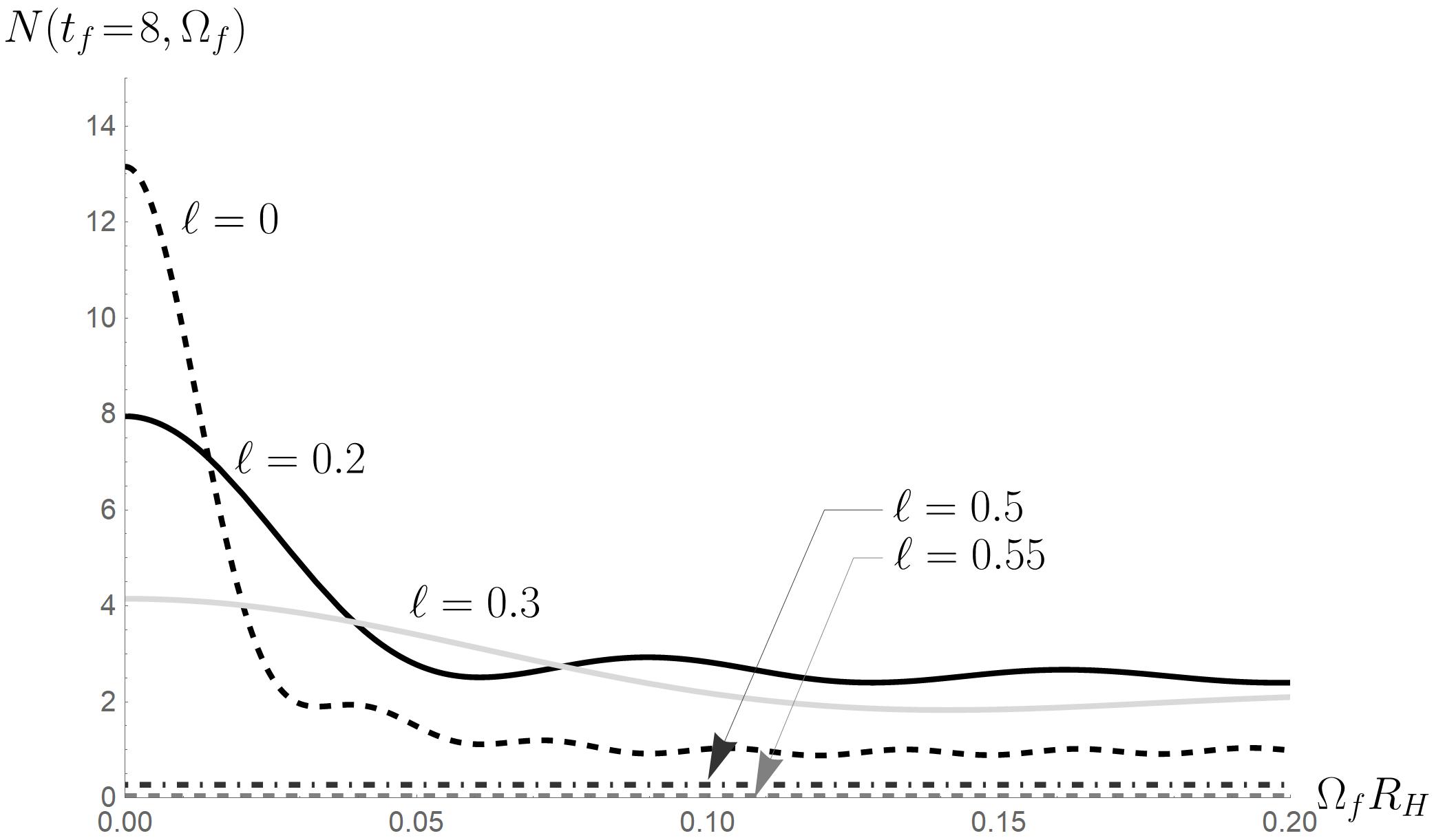
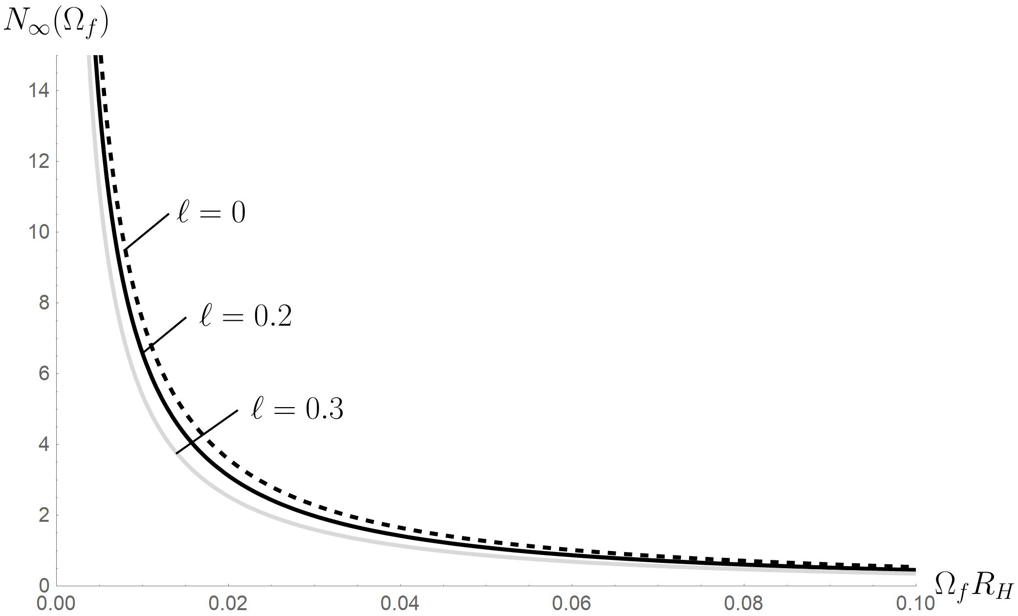
Figure 1: The occupation number (59) for a finite time is plotted in Fig. 1(a). Figure 1(b) also shows the spectrum of Eq. (65) which is the occupation number with the infinite time. Note that $\Omega_{f}R_{H}$ is a dimensionless quantity, and we can set $R_{H}=1$ for simplicity. In Figs. 1(a) and 1(b), the black and the grey curves are for the Hayward black hole with $\ell=0.2$ and $\ell=0.3$, respectively, and the dashed curves are for the Schwarzschild black hole where $\ell=0$. Thus, in Fig. 1(a), the low-lying black dot-dashed curve ($\ell=0.5$) and the grey dashed curve ($\ell=0.55$) are for the occupation number of the Hayward black hole close to the extremal limit $(\ell=\ell_{\max}\approx 0.577)$.

Likewise, the spectrum of the occupation number in the Hayward black hole can also be calculated from Eqs. (38) and (57) as

$$N\left(\eta_{f},\omega_{f}\right)=\left.\frac{1}{4}\omega_{f}\zeta^{2}\left[\left(1-\frac{1}{\omega_{f}\zeta^{2}}\right)^{2}+\frac{1}{\omega_{f}^{2}\zeta^{2}}\left(\frac{\textrm{d}\zeta}{\textrm{d}\eta}\right)^{2}\right]\right|_{\omega_{0}=\sqrt{1-H\eta_{f}}\omega_{f}}.$$ (58)

By using Eq. (26), a frequency for the original time $t$ can be defined as $\Omega(t)=(\textrm{d}\eta/\textrm{d}t)\omega(\eta)=f(R)\omega(\eta)$, so the occupation number (58) can be written in terms of $t_{f}$ and $\Omega_{f}$ as Kolopanis:2013sty

$$N(t_{f},\Omega_{f})=\frac{1}{4}e^{\frac{1}{2}Ht_{f}}\left(\xi^{2}+\chi^{2}\right)\left[\left(1-\frac{1}{e^{\frac{1}{2}Ht_{f}}(\xi^{2}+\chi^{2})}\right)^{2}+\left(\frac{He^{-Ht_{f}}}{\Omega_{f}}\frac{\xi\dot{\xi}+\chi\dot{\chi}}{\xi^{2}+\chi^{2}}\right)^{2}\right],$$ (59)

where $\Omega_{f}\approx e^{-Ht_{f}}\omega_{f}$ with $\dot{\xi}=\textrm{d}\xi/\textrm{d}\tilde{\eta}$ and $\dot{\chi}=\textrm{d}\chi/\textrm{d}\tilde{\eta}$.

On the other hand, in order to study the limiting case we rewrite the occupation number (59) in terms of $x$ and $y$ for convenience as

$$N(x,y)=\frac{x}{4y}\left(\xi^{2}+\chi^{2}\right)\left(1-\frac{1}{(x/y)(\xi^{2}+\chi^{2})}\right)^{2}+\frac{1}{y^{4}}\frac{\{x(\xi h_{1}+\chi h_{2})\}^{2}}{(x/y)(\xi^{2}+\chi^{2})},$$ (60)

where

$$h_{1}(x,y) =e^{-Ht_{f}}\dot{\xi}=-\frac{\pi y^{2}}{4}\{Y_{0}(x)J_{0}(y)-J_{0}(x)Y_{0}(y)\},$$ (61)

$$h_{2}(x,y) =e^{-Ht_{f}}\dot{\chi}=-\frac{\pi y^{2}}{4}\{Y_{1}(x)J_{0}(y)-J_{1}(x)Y_{0}(y)\}.$$ (62)

In the incipient limit, $x$ and $y$ are approximately $x\approx 2\Omega_{f}e^{Ht_{f}/2}/H$ and $y\approx 2\Omega_{f}/H$, respectively. Using the asymptotic forms of Bessel functions in the limit $t_{f}\to\infty$, we get

$$\frac{x}{y}(\xi^{2}+\chi^{2}) \to\frac{\pi y}{2}\{J_{1}^{2}(y)+Y_{1}^{2}(y)\},$$ (63)

$$x\left(\xi h_{1}+\chi h_{2}\right) \to-\frac{\pi y^{3}}{4}\{J_{0}(y)J_{1}(y)+Y_{0}(y)Y_{1}(y)\}.$$ (64)

From Eqs. (63) and (64), the occupation number (60) for $t_{f}\to\infty$ is obtained as

$$N_{\infty}(\Omega_{f})=\frac{\pi}{8}\frac{y}{J_{1}^{2}(y)+Y_{1}^{2}(y)}\left[\left(\!\!J_{1}^{2}(y)+Y_{1}^{2}(y)\!-\!\frac{2}{\pi y}\right)^{2}+\{J_{0}(y)J_{1}(y)+Y_{0}(y)Y_{1}(y)\}^{2}\right].$$ (65)

The spectrum of the occupation number in terms of $\Omega_{f}$ for a finite time and the infinite time are shown in Fig. 1 and Fig. 1. The radiation at early times in Fig. 1 turns out to be nonthermal; however, the spectrum in Fig. 1 is very close to the thermal Hawking distribution if the shell approaches its own horizon. In particular, in Fig. 1, we can find that the number of quanta at a low frequency decreases when $\ell$ is getting larger. Extremely, if $\ell\to\ell_{\max}=4M/(3\sqrt{3})$, the occupation number (59) eventually vanishes because $H=(R_{H}^{2}-3\ell^{2})/R_{H}^{3}$ approaches zero with $R_{H}=1$. We can show easily $N(x,y)\to 0$ by using the following limits:

$$(x/y)(\xi^{2}+\chi^{2})\to 1,\qquad(x/y^{2})(\xi h_{1}+\chi h_{2})\to 0,$$ (66)

which are obtained from the asymptotic forms of Bessel functions as $H\to 0$, i.e., $x\to\infty$ and $y\to\infty$. The plotting for this result can also be found in Fig. 1; the occupation number is getting smaller as $\ell$ is getting closer to $\ell_{\max}=1/\sqrt{3}\approx 0.577$ ($R_{H}=1$). This extremal limit looks similar to the fact that the Hawking radiation vanishes for extremal black holes.

Our results are quite similar to those of the Reissner-Nordström (RN) domain wall in Ref. Greenwood:2009pd . The author in Ref. Greenwood:2009pd showed that the spectrum of the occupation number is nonthermal, but it becomes more and more thermal as $t_{f}\to\infty$. In addition, in the extremal case the temperature seen by the asymptotic observer goes to zero when the shell crosses the horizon. These similarities are due to the fact that the spacetime structure of Eq. (1) is analogous to that of the RN domain wall in that they share two horizons and asymptotic flatnesses. However, there are two differences between our analysis and that of the RN domain wall: the methodology and the type of a scalar field. Firstly, the author in Ref. Greenwood:2009pd found “best fit temperatures” $\beta^{-1}$ for a finite time by fitting $\beta\omega_{f}$ to $\log{(1+1/N)}$, whereas we investigated the occupation number analytically for infinite time as well as a finite time. Thus, we could read off the Hawking temperature of the Hayward black hole at infinite time analytically. Secondly, a complex scalar field which represents charged particles and antiparticles was considered in order to investigate the effect of charge $Q(Q>0)$ of the RN black hole. The occupation number for the particles (or antiparticles) with a negative charge was shown to be subdominant to that with a positive charge because of the Coulomb repulsion. However, we considered the real scalar field $\Phi$ for neutral particles, so there exists one kind of the occupation number. Moreover, instead of $Q$, the effect of $\ell$ appears as shown in Fig. 1 and Fig. 1. Essentially, the above differences came from the fact that the Hayward black hole is neutral unlike the RN black hole in spite of similar spacetime structures.

Now, we can read off a temperature in a low frequency region. In the low frequency $\Omega\ll 1$, Eq. (65) is approximated as

$$N_{\infty}(\Omega_{f})\approx\frac{H}{4\pi\Omega_{f}},$$ (67)

and the Planckian distribution can also be written as

$$N_{\textrm{Planck}}(\Omega)=\frac{1}{e^{\frac{\Omega}{T}}-1}\approx\frac{T}{\Omega}.$$ (68)

Comparing Eq. (67) and Eq. (68), we can obtain the temperature

$$T=\frac{H}{4\pi}$$ (69)

which is the same as the Hawking temperature of the Hayward black hole.

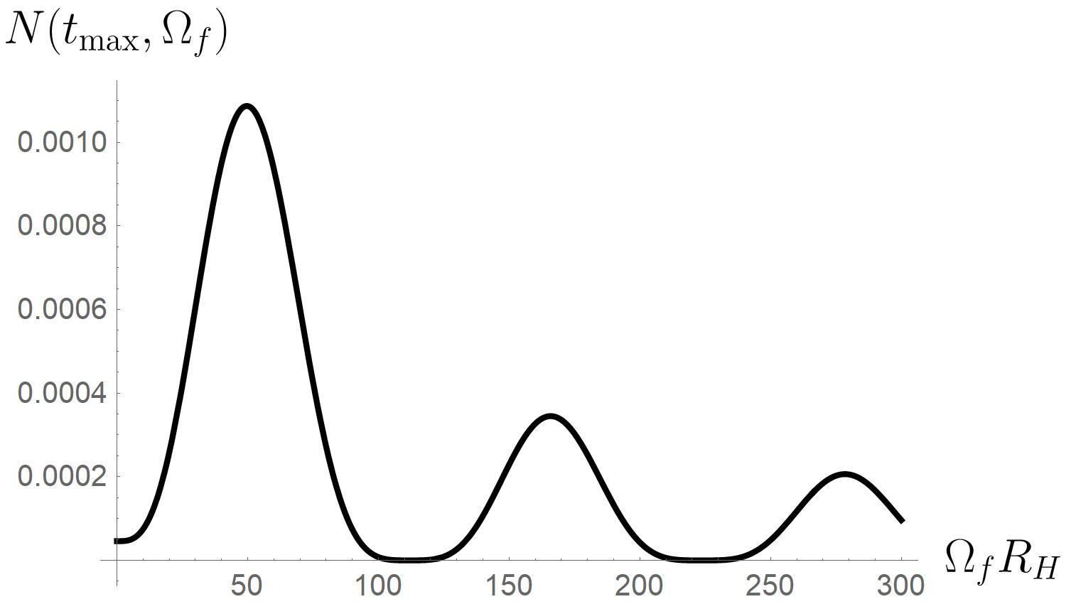
Figure 2: The occupation number (70) for the final time $t_{\max}\approx 0.028$ ($R_{0}=0.02$) is plotted with $\tilde{H}\approx 0.95$, $\ell=0.6$, and $R_{H}=1$. The occupation number is damped oscillating, which is different from the thermal Hawking distribution.

On the other hand, in the case of $M<M^{*}$, the occupation number can also be calculated from the analytic solution (53), which is given as

$$N\left(t_{f},\Omega_{f}\right)=\left.\frac{1}{4}\Omega_{f}\bar{\zeta}^{2}\left[\left(1-\frac{1}{\Omega_{f}\bar{\zeta}^{2}}\right)^{2}+\frac{1}{\Omega_{f}^{2}\bar{\zeta}^{2}}\left(\frac{\textrm{d}\bar{\zeta}}{\textrm{d}t}\right)^{2}\right]\right|_{\Omega_{0}=\sqrt{1-\tilde{H}t_{f}}\Omega_{f}},$$ (70)

where $\Omega_{0}=\sqrt{\tilde{b}_{0}}$ and $\Omega_{f}=\Omega_{0}/\sqrt{1-\tilde{H}t}$ with $\tilde{H}=\tilde{b}_{1}/\tilde{b}_{0}$. Thus, the spectrum of the occupation number in terms of $\Omega_{f}$ for the final time $t_{\max}=\sqrt{2}R_{0}$ is plotted in Fig. 2. Note that it takes a finite time during the collapsing and the spectrum even for the final time $t_{\max}$ is not close to the thermal Hawking distribution in contrast to the spectrum in Fig. 1.

V conclusion

We studied the collapsing shell to form the Hayward black hole and investigated the quantum radiation. Using the Israel formulation, we obtained the mass relation between the energy density of the shell and the mass of the Hayward black hole. The main difference from the Schwarzschild black hole is that the energy density in the exterior region of the shell as well as the energy density on the shell contributes to the source of the Hayward black hole. Next, we investigated the quantum radiation from the shell by employing the functional Schrödinger equation in cases of $M>M^{*}$ and $M<M^{*}$. In $M>M^{*}$ when the shell forms the Hayward black hole, the equation takes the form of the harmonic oscillator with time-dependent frequency. From the vacuum state defined by the coherent states, the density matrix, the probability current, and the occupation number were exactly calculated. By using these quantities, we showed that the process of the radiation is unitary during the collapsing. For $M<M^{*}$, we derived the functional Schrödinger equation for a small radius which corresponds to the incipient limit in the former case ($M>M^{*}$). In this case, all terms in the exterior and interior actions appear in the quantized Hamiltonian and then, the functional Schrödinger equation is given by the form of the harmonic oscillator with the time-dependent mass and frequency. For a certain small time satisfying some constraints, we could find the analytic solution of the equation. Next, we investigated the spectrum of the radiation in the case of $M>M^{*}$ when the shell finally forms the Hayward black hole. The spectrum does not coincide with the thermal Hawking radiation at early times; however, it is very close to the thermal Hawking distribution when the shell approaches the horizon. For the infinite time, the temperature of the radiation could be estimated in the limit of the low frequency, and it turned out to be the Hawking temperature of the Hayward black hole. In addition, the number of quanta at a low frequency decreases for a larger value of $\ell$. In the extremal limit of $\ell\to\ell_{\max}$, the occupation number (59) eventually vanishes, which is reminiscent of the extremal limit of black holes where the Hawking radiation vanishes. Moreover, the occupation number for $M<M^{*}$ was studied, and thus, it turned out to be nonthermal even for the final time when the shell approaches the origin.

Finally, we comment on the incipient limit $R\to R_{H}$ employed in our paper. In the incipient limit, we would get the simplified analytic results such as Eqs. (19) and (32), so we could easily show that the whole process of the collapsing must be unitary because $\operatorname{Tr}\rho=1$ regardless of $\eta$ in Eq. (40). However, the incipient limit corresponds to the moment when the shell approaches the horizon, that is, almost the final stage of the collapsing. If the incipient limit is released, then the vacuum state (29) will be modified. Although we expect that this modification of the vacuum state will not affect the final results in our paper, it deserves further study.