Revisiting $X(3872)\to D^{0}\bar{D}^{0}\pi^{0}$ in XEFT

Abstract

The calculation of the decay $X(3872)\to D^{0}\bar{D}^{0}\pi^{0}$ in effective field theory is revisited to include final state $\pi^{0}D^{0}$, $\pi^{0}\bar{D}^{0}$and $D^{0}\bar{D}^{0}$ rescattering diagrams. These introduce significant uncertainty into the prediction for the partial width as a function of the binding energy. The differential distribution in the pion energy is also studied for the first time. The normalization of the distribution is again quite uncertain due to higher order effects but the shape of the distribution is unaffected by higher order corrections. Furthermore the shape of the distribution and the location of the peak are sensitive to the binding energy of $X(3872)$. The shape is strongly impacted by the presence of virtual $D^{*0}$ graphs which highlights the molecular nature of the $X(3872)$. Measurement of the pion energy distribution in the decay $X(3872)\to D^{0}\bar{D}^{0}\pi^{0}$ can reveal interesting information about the binding nature of the $X(3872)$.

I Introduction

The $X(3872)$ Abe et al. (2003) is the first of many exotic charmonium and bottomonium states found in various high energy experiments since 2003. For reviews of these so-called $XYZ$ mesons and related exotic states, see Refs. Chen et al. (2016); Richard (2016); Esposito et al. (2016); Hosaka et al. (2016); Lebed et al. (2017); Guo et al. (2018); Ali et al. (2017); Olsen et al. (2018); Kou et al. (2018); Cerri et al. (2018); Liu et al. (2019); Brambilla et al. (2019), and for a review dedicated to the $X(3872)$, see Ref. Kalashnikova and Nefediev (2019). The quantum numbers of the $X(3872)$ have been determined to be $J^{PC}=1^{++}$Aaij et al. (2013), which is consistent with it being a $\chi_{c1}$ state (and it is thus called $\chi_{c1}(3872)$ in the Review of Particle Physics (RPP) Tanabashi et al. (2018), which reflects its quantum numbers without reference to the internal structure). A striking fact about the $X(3872)$ is that it is essentially degenerate with the $D^{*0}\bar{D}^{0}$ threshold. Currently, the particle data group has the $X(3872)$ mass being degenerate with $m_{D^{*0}}+m_{D^{0}}$ with an uncertainty of about 0.2 MeV. Therefore, the $X(3872)$ couples strongly to this channel and its wavefunction should contain a significant component of weakly bound $D^{*0}\bar{D}^{0}$ (plus the charge conjugate channel, which will be implied in what follows). Because of this it is widely believed that the $X(3872)$ is a hadronic molecule composed of $D^{*0}\bar{D}^{0}$.

If the $X(3872)$ is a weakly coupled bound state of $D^{*0}\bar{D}^{0}$ then ideas of effective range theory (ERT) can be applied to its decays. Voloshin used ERT to compute the decays $X(3872)\to D^{0}\bar{D}^{0}\pi^{0}$ and $X(3872)\to D^{0}\bar{D}^{0}\gamma$ Voloshin (2004). For the former decay, the partial width for $X(3872)$ was predicted as a function of the binding energy, which was much more uncertain at the time of that publication. In the limit of zero binding energy the $D^{*0}$ in the $X(3872)$ is at rest and the partial width for $X(3872)\to D^{0}\bar{D}^{0}\pi^{0}$ is equal to that for $\Gamma[D^{*0}\to D^{0}\pi^{0}]=36.4\pm 0.98$ keV. For the current constraints on the binding energy the $X(3872)$ should be very close to this limit. However, it is difficult to test this prediction as the total width is only weakly constrained, $\Gamma[X(3872)]<1.2$ MeV, and the branching fraction to $D^{0}\bar{D}^{0}\pi^{0}$ only is constrained to be greater than 40% in the RPP Tanabashi et al. (2018).

ERT can be systematically improved upon using effective field theory (EFT). For the $X(3872)$ the relevant effective theory is XEFT Fleming et al. (2007). In this theory the relevant degrees of freedom are the $D^{0}$, $\bar{D}^{0}$, $D^{*0}$, $\bar{D}^{*0}$, and $\pi^{0}$, all treated non-relativistically. In Ref. Fleming et al. (2007), XEFT was used to calculate the partial width for the decay $X(3872)\to D^{0}\bar{D}^{0}\pi^{0}$. The ERT prediction for $X(3872)\to D^{0}\bar{D}^{0}\pi^{0}$ emerges as the leading order in XEFT, and corrections from pion loops, range corrections, and higher dimension operators in the effective Lagrangian can be treated systematically. In XEFT pions can be treated perturbatively, and Ref. Fleming et al. (2007) found that pion loops gave very small corrections to the decay. By varying the effective range and coefficients of other operators, Ref. Fleming et al. (2007) was able to estimate the uncertainty in the ERT prediction for the partial width as a function of binding energy. For other applications of XEFT see Refs.Fleming and Mehen (2008, 2012); Mehen and Springer (2011); Margaryan and Springer (2013); Braaten et al. (2010); Canham et al. (2009); Jansen et al. (2014, 2015); Mehen (2015); Alhakami and Birse (2015); Braaten (2015). For other EFT approaches to the $X(3872)$ see Refs. AlFiky et al. (2006); Baru et al. (2011); Valderrama (2012); Nieves and Valderrama (2012); Baru et al. (2013); Guo et al. (2013a, b); Baru et al. (2015); Schmidt et al. (2018).

In Ref. Guo et al. (2018), it was pointed out that operators contributing to $\pi$-$D$ scattering lengths give rise to diagrams that are the same order in the power counting as those considered in Ref. Fleming et al. (2007). The relevant operators were first written down in Refs. Guo et al. (2008, 2009), which came after Ref. Fleming et al. (2007). The $\pi$-$D$ scattering lengths have been determined from recent lattice studies Liu et al. (2013); Mohler et al. (2013, 2013); Guo et al. (2019), and part of the goal of this paper is to calculate the impact they have on the prediction for the partial width of the $X(3872)$ in XEFT. In addition we also include $D^{0}\bar{D}^{0}$ rescattering effects, these were first studied in Ref. Guo et al. (2014). We find that including these effects doubles the uncertainty in the prediction for the partial width found in Ref. Fleming et al. (2007). The theoretical uncertainty in the prediction for the partial width is rather large, for example, it is ${}^{+50}_{-30}\%$ for a binding energy of $0.2$ MeV.

In this paper, we also calculate the differential spectrum, $d\Gamma[X(3872)\to D^{0}\bar{D}^{0}\pi^{0}]/dE_{\pi}$, where $E_{\pi}$ is the pion energy, for the first time. While the normalization of this rate suffers similar uncertainties, the shape of this distribution does not. Interestingly, this shape is sensitive to the binding energy and the molecular nature of the $X(3872)$. The distribution becomes more narrowly peaked near the maximal pion energy as the binding energy goes to zero. The location of the peak is insensitive to higher order corrections. The shape of the distribution is sensitive to the molecular nature of the $X(3872)$ because the $X(3872)$ couples to the final state through a virtual $D^{*0}$ propagator which is largest when the momentum of either $D$ meson in the final state goes to zero. The propagator has a pole at $p_{D}^{2}=-\gamma^{2}$ and $p_{\bar{D}}^{2}=-\gamma^{2}$, where $p_{D}$, $p_{\bar{D}}$ and $\gamma$ are the $D$ meson momentum, $\bar{D}$ meson momentum, and $X(3872)$ binding momentum, respectively. Thus, effect becomes more dramatic as the binding energy goes to zero. Amplitudes without the $D^{*}$ pole lead to broad $E_{\pi}$ distributions peaked at lower energy.

In the next section we briefly review XEFT as is relevant for our analysis and give the NLO amplitudes explicitly. In Section III we show the results of the calculations of the partial width and and the differential distribution in $E_{\pi}$. In Section IV we give our conclusions.

II NLO Partial Decay Amplitudes of $X(3872)$

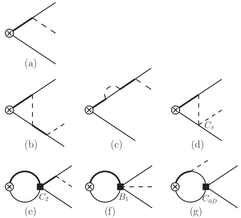
Figure 1: Feynman diagrams (reprinted from Refs. Guo et al. (2018); Fleming et al. (2007)) up to NLO for calculating the partial decay width of $X(3872)\to D^{0}\bar{D}^{0}\pi^{0}$. The circled cross is the $X(3872)$ field insertion. The thin solid, thick solid, and dashed lines represent $D^{0}(\bar{D}^{0})$, $D^{*0}(\bar{D}^{*0})$, and $\pi^{0}$, respectively.

XEFT Fleming et al. (2007) combines heavy hadron chiral perturbation theory Wise (1992); Burdman and Donoghue (1992); Yan et al. (1992) with the Kaplan–Savage–Wise approach to describing low energy nucleon-nucleon interactions Kaplan et al. (1998a, b). Similar effective theories have been developed for other possible hadronic molecules which are located very close to thresholds, for example, $Z_{b}(10610)$ and $Z_{b}(10650)$ Mehen and Powell (2011, 2013) and the $Z_{c}(3900)$ Wilbring et al. (2013). For a more detailed discussion of XEFT we refer the readers to the original work in Ref. Fleming et al. (2007). Here we simply quote the XEFT Lagrangian and comment on the power counting of Feynman diagrams relevant for our present analysis.

The XEFT Lagrangian we use to calculate the partial decay rate of $X(3872)$ $\to$ $D^{0}\bar{D}^{0}\pi^{0}$ is Fleming et al. (2007); Guo et al. (2018)

$${\cal L} = \sum_{\bm{\phi}=\bm{D},\bm{{\bar{D}}}}\bm{\phi}^{\dagger}\bigg{(}i\partial_{0}+\frac{\bm{\nabla}^{2}}{2M_{D^{*0}}}\bigg{)}\bm{\phi}+\sum_{{\phi}=D,\bar{D}}\phi^{\dagger}\bigg{(}i\partial_{0}+\frac{\bm{\nabla}^{2}}{2M_{D^{0}}}\bigg{)}\phi+\pi^{\dagger}\bigg{(}i\partial_{0}+\frac{\bm{\nabla}^{2}}{2M_{\pi^{0}}}+\delta\bigg{)}\pi$$ (1)

$$+\left[\frac{\bar{g}}{F_{\pi}}\frac{1}{\sqrt{2M_{\pi^{0}}}}\left(D\bm{D}^{\dagger}\cdot\bm{\nabla}\pi+\bar{D}^{\dagger}\bm{{\bar{D}}}\cdot\bm{\nabla}\pi^{\dagger}\right)+{\rm h.c.}\right]$$

$$-\,\frac{C_{0}}{2}\,\left(\bm{{\bar{D}}}D+\bm{D}\bar{D}\right)^{\dagger}\cdot\left(\bm{{\bar{D}}}D+\bm{D}\bar{D}\right)$$

$$+\left[\frac{C_{2}}{16}\,\left(\bm{{\bar{D}}}D+\bm{D}\bar{D}\right)^{\dagger}\cdot\left(\bm{{\bar{D}}}(\overleftrightarrow{\nabla})^{2}D+\bm{D}(\overleftrightarrow{\nabla})^{2}\bar{D}\right)+{\rm h.c.}\right]$$

$$+\left[\frac{B_{1}}{\sqrt{2}}\frac{1}{\sqrt{2M_{\pi^{0}}}}\left(\bm{{\bar{D}}}D+\bm{D}\bar{D}\right)^{\dagger}\cdot D\bar{D}\bm{\nabla}\pi+{\rm h.c.}\right]$$

$$+\frac{C_{\pi}}{2M_{\pi^{0}}}\left(D^{\dagger}\pi^{\dagger}D\pi+\bar{D}^{\dagger}\pi^{\dagger}\bar{D}\pi\right)+C_{0D}D\,^{\dagger}\bar{D}^{\dagger}D\bar{D}\,,$$

where $\delta=\Delta-M_{\pi^{0}}\simeq 7.0$ MeV with $\Delta=M_{D^{*0}}-M_{D^{0}}$, the pion decay constant is $F_{\pi}=91.9$ MeV, the coupling between pions and charmed mesons $\bar{g}\simeq 0.27$ fixed from the updated $D^{*+}$ decay width Tanabashi et al. (2018), and $\overleftrightarrow{\nabla}=\overleftarrow{\nabla}-\overrightarrow{\nabla}$. The last line of Eq. (1) gives rise to $\pi^{0}D^{0}(\bar{D}^{0})$ and $D^{0}\bar{D}^{0}$ rescattering which were not considered in the original Ref. Fleming et al. (2007). The Feynman diagrams up to NLO that are relevant to the partial decay rate of $X(3872)$ $\to$ $D^{0}\bar{D}^{0}\pi^{0}$ are shown in Fig. 1.

To justify the necessity of including the $\pi^{0}D^{0}(\bar{D}^{0})$ and $D^{0}\bar{D}^{0}$ rescattering diagrams in studying the partial decay width of $X(3872)$ $\to$ $D^{0}\bar{D}^{0}\pi^{0}$, we review the power counting of Feynman diagrams in Fig. 1 that was already discussed in detail in Ref. Fleming et al. (2007) and Ref. Guo et al. (2018). The relevant momenta involved in the decay dynamics are $\{p_{D},p_{D^{*}},p_{\pi},\gamma,\mu\}$ where $\gamma$ is the binding momentum, $\sqrt{2\mu_{0}B_{X}}$, with $B_{X}$ is the binding energy and $\mu=\sqrt{\Delta^{2}-M^{2}_{\pi^{0}}}$. These momenta are the same order, which we generically denote as $Q$ which is also the power counting parameter. For the diagrams in Fig. 1, each pion vertex contributes a factor of $Q$, each propagator $Q^{-2}$, and each loop integral $Q^{5}$. It was argued in Ref. Fleming et al. (2007) that $C_{0}$ scales as $Q^{-1}$ which is responsible for the formation of $X(3872)$ bound state, and that $C_{2}$ and $B_{1}$ both scale as $Q^{-2}$ and together can be parameterized in terms of the effective range in $D^{*0}\bar{D}^{0}$ (or $\bar{D}^{*0}{D}^{0}$) scattering. The power counting of $C_{\pi}$ and $C_{0D}$ was discussed in Ref. Guo et al. (2018). The $C_{\pi}$ contact term can be obtained by matching to the Heavy Hadron Chiral Lagrangian Burdman and Donoghue (1992); Wise (1992); Yan et al. (1992); Guo et al. (2008). The NLO investigation of the $\pi^{0}D^{0}\to\pi^{0}D^{0}$ scattering indicates (using $D_{s}$ and $D$ mass splitting and lattice data) that the NLO amplitude ${\cal A}(\pi^{0}D^{0}\to\pi^{0}D^{0})$ is of order one, i.e., $C_{\pi}\sim Q^{0}$ Guo et al. (2008, 2009). If $C_{0D}$ is assumed to be of order $Q^{0}$ as a natural choice, then the NLO diagram from $D^{0}\bar{D}^{0}$ rescattering (diagram (g) in in Fig. 1) scales as $Q^{0}$. On the other hand, if $D^{0}\bar{D}^{0}$ rescattering becomes non-perturbative, then $C_{0D}$ scales as $Q^{-1}$ which is similar to the scaling of $C_{0}$ discussed above and which gives even more significant contribution to the decay of $X(3872)$. With these basic scaling rules in hand, it is straightforward to check, in Fig. 1, that LO diagram (a) scales as $Q^{-1}$ and NLO diagrams (b)–(f) scale as $Q^{0}$. In addition, depending on whether $C_{0D}$ scales as $Q^{0}$ or $Q^{-1}$, diagram (g) scales as $Q^{0}$ or $Q^{-1}$.

Next, we list all the decay amplitudes of $X(3872)$ up to NLO, all of which are derived in the rest frame of the $X(3872)$. The LO amplitude from the tree-level diagram (a) in Fig. 1 is

$$i\mathcal{A}_{\text{LO}} = \frac{\bar{g}\,\mu_{0}}{F_{\pi}\sqrt{M_{\pi^{0}}}}\vec{p}_{\pi}\cdot\vec{\epsilon}_{X}\left(\frac{1}{\vec{p}_{D}^{\,2}+\gamma^{2}}+\frac{1}{\vec{p}_{\bar{D}}^{\,2}+\gamma^{2}}\right),$$ (2)

where $\mu_{0}$ is the reduced mass of the neutral $D$ and $D^{*}$ pair, $\vec{p}_{D(\bar{D})}$ is the 3-momentum of the external $D^{0}(\bar{D}^{0})$, $\vec{p}_{\pi}$ is the momentum of the final state $\pi^{0}$, $\vec{\epsilon}_{X}$ is the polarization vector of the $X(3872)$, and $\gamma$ is the binding momentum.

The amplitude for diagram (b) in Fig. 1 is given by

$$i\mathcal{A}_{\text{(b)}} = -\frac{\bar{g}^{3}}{4F_{\pi}^{3}M_{\pi^{0}}^{3/2}}\bigg{\{}\frac{2\mu_{0}}{\vec{p}_{D}^{\,2}+\gamma^{2}}\Big{[}\vec{p}_{D}^{\,2}\vec{p}_{\pi}\cdot\vec{\epsilon}_{X}I_{1}^{(2)}(p_{D})+\vec{p}_{D}\cdot\vec{p}_{\pi}\vec{p}_{D}\cdot\vec{\epsilon}_{X}\Big{(}I(p_{D})-2I^{(1)}(p_{D})+I_{0}^{(2)}(p_{D})\Big{)}\Big{]}$$ (3)

$$+\frac{2\mu_{0}}{\vec{p}_{\bar{D}}^{\,2}+\gamma^{2}}\Big{[}\vec{p}_{\bar{D}}^{\,2}\vec{p}_{\pi}\cdot\vec{\epsilon}_{X}I_{1}^{(2)}(p_{\bar{D}})+\vec{p}_{\bar{D}}\cdot\vec{p}_{\pi}\vec{p}_{\bar{D}}\cdot\vec{\epsilon}_{X}\Big{(}I(p_{\bar{D}})-2I^{(1)}(p_{\bar{D}})+I_{0}^{(2)}(p_{\bar{D}})\Big{)}\Big{]}\bigg{\}}\,,$$

The loop integrals $I(p)$, $I^{(1)}(p)$, and $I^{(2)}_{0,1}(p)$ are defined in Appendix A, and $m_{1}$, $m_{2}$ and $m_{3}$ should be replaced by the mass of $D^{*0}$, $D^{0}$ and $\pi^{0}$, respectively.

Diagram (c) in Fig. 1 does not contribute to the NLO calculation of the decay of $X(3872)\to D^{0}\bar{D}^{0}\pi^{0}$ Fleming et al. (2007). This is because the $D^{*0}$ and $\bar{D}^{*0}$ residual mass counterterms cancel the real part of diagram (c) while the imaginary part does not contribute at NLO since the LO diagram (a) is purely real.

The amplitude for diagram (d) in Fig. 1 is given by

$$i\mathcal{A}_{\text{(d)}}=\frac{\bar{g}C_{\pi}}{4F_{\pi}M_{\pi^{0}}^{3/2}}\Big{\{}\vec{p}_{D}\cdot\vec{\epsilon}_{X}\left[I(p_{D})-I^{(1)}(p_{D})\right]+\vec{p}_{\bar{D}}\cdot\vec{\epsilon}_{X}\left[I(p_{\bar{D}})-I^{(1)}(p_{\bar{D}})\right]\Big{\}}.$$ (4)

Again the loop integrals $I(p)$ and $I^{(1)}(p)$ are defined in Appendix A, where $m_{1}$, $m_{2}$ and $m_{3}$ should be replaced by the mass of $D^{*0}$, $D^{0}$ and $\pi^{0}$, respectively.

The amplitude for diagram (e) reads

$$i\mathcal{A}_{\text{(e)}}=-C_{2}\frac{\bar{g}\mu_{0}^{2}}{4\pi F_{\pi}\sqrt{M_{\pi^{0}}}}\left(\Lambda_{\text{PDS}}-\gamma\right)\vec{p}_{\pi}\cdot\vec{\epsilon}_{X}\left(\frac{\vec{p}_{\bar{D}}^{\,2}-\gamma^{2}}{\vec{p}_{\bar{D}}^{\,2}+\gamma^{2}}+\frac{\vec{p}_{D}^{\,2}-\gamma^{2}}{\vec{p}_{D}^{\,2}+\gamma^{2}}\right),$$ (5)

where $\Lambda_{\text{PDS}}$ is the scale introduced in the power divergence subtraction (PDS) scheme Kaplan et al. (1998a) to regularize the ultraviolet (UV) divergence in the two-point bubble diagram, see Appendix A.

The amplitude for diagram (f) reads

$$i\mathcal{A}_{\text{(f)}}=B_{1}\frac{\mu_{0}}{2\pi\sqrt{2M_{\pi^{0}}}}\left(\Lambda_{\text{PDS}}-\gamma\right)\vec{p}_{\pi}\cdot\vec{\epsilon}_{X}.$$ (6)

The amplitude for diagram (g) in Fig. 1 is given by

$$i\mathcal{A}_{\text{(g)}}=\frac{\bar{g}C_{0D}}{F_{\pi}\sqrt{M_{\pi^{0}}}}\vec{p}_{\pi}\cdot\vec{\epsilon}_{X}I(p_{\pi})\,.$$ (7)

Here the loop integral $I(p)$ is as that defined in Appendix A, where $m_{1}$, $m_{2}$ and $m_{3}$ should be replaced by the mass of $D^{*0}$, $D^{0}$ and $D^{0}$, respectively.

III Implications of $\pi^{0}D^{0}$ and $D^{0}\bar{D}^{0}$ rescattering

In this section, we numerically investigate the $\pi^{0}D^{0}$ and $D^{0}\bar{D}^{0}$ rescattering effects for the partial decay of $X(3872)\to D^{0}\bar{D}^{0}\pi^{0}$. The differential decay rate is

$$\frac{d\Gamma_{\mathrm{NLO}}}{dp_{D}^{2}dp_{\bar{D}}^{2}}=\frac{d\Gamma_{\mathrm{LO}}}{dp_{D}^{2}dp_{\bar{D}}^{2}}\left(1+\frac{\bar{g}^{2}\mu_{0}\gamma}{3\pi F_{\pi}^{2}}\left(\frac{4\gamma^{2}-\mu^{2}}{4\gamma^{2}+\mu^{2}}\right)+C_{2}\left(\Lambda_{\mathrm{PDS}}\right)\frac{\mu_{0}\gamma\left(\gamma-\Lambda_{\mathrm{PDS}}\right)^{2}}{\pi}\right)$$

$$-\frac{\bar{g}\gamma}{8\sqrt{2}\pi^{3}F_{\pi}}\left(\sqrt{2}\frac{\bar{g}\mu_{0}}{F_{\pi}}C_{2}\left(\Lambda_{\mathrm{PDS}}\right)-B_{1}\left(\Lambda_{\mathrm{PDS}}\right)\right)\left(\Lambda_{\mathrm{PDS}}-\gamma\right)\left(\vec{p}_{\pi}\cdot\vec{\epsilon}_{X}\right)^{2}\left(\frac{1}{p_{D}^{2}+\gamma^{2}}+\frac{1}{p_{\bar{D}}^{2}+\gamma^{2}}\right)$$

$$+\frac{1}{8\pi^{2}}\frac{\bar{g}^{4}}{F_{\pi}^{4}}\frac{\gamma}{M_{\pi^{0}}}\left[\left(\vec{p}_{\pi}\cdot\vec{\epsilon}_{X}\right)^{2}\left(\frac{1}{p_{D}^{2}+\gamma^{2}}+\frac{1}{p_{\bar{D}}^{2}+\gamma^{2}}\right)\left(\frac{p_{D}^{2}{I}_{1}^{(2)}\left(p_{D}\right)}{P_{D}^{2}+\gamma^{2}}+\frac{p_{\bar{D}}^{2}{I}_{1}^{(2)}\left(p_{\bar{D}}\right)}{P_{\bar{D}}^{2}+\gamma^{2}}\right)\right]$$

$$+\frac{1}{8\pi^{2}}\frac{\bar{g}^{4}}{F_{\pi}^{4}}\frac{\gamma}{M_{\pi^{0}}}\left[\vec{p}_{\pi}\cdot\vec{\epsilon}_{X}\left(\frac{1}{p_{D}^{2}+\gamma^{2}}+\frac{1}{p_{\bar{D}}^{2}+\gamma^{2}}\right)\left(\frac{\vec{p}_{D}\cdot\vec{\epsilon}_{X}\vec{p}_{D}\cdot\vec{p}_{\pi}}{p_{D}^{2}+\gamma^{2}}\left(I(p_{D})-2I^{(1)}(p_{D})+I^{(2)}_{0}(p_{D})\right)\right.\right.$$

$$+\left.\left.\frac{\vec{p}_{\bar{D}}\cdot\vec{\epsilon}_{X}\vec{p}_{\bar{D}}\cdot\vec{p}_{\pi}}{p_{\bar{D}}^{2}+\gamma^{2}}\left(I(p_{\bar{D}})-2I^{(1)}(p_{\bar{D}})+I^{(2)}_{0}(p_{\bar{D}})\right)\right)\right]$$

$$+\frac{C_{\pi}\bar{g}^{2}\gamma\,\vec{p}_{\pi}\cdot\vec{\epsilon}_{X}}{16\pi^{2}F_{\pi}^{2}M_{\pi^{0}}\mu_{0}}\left(\frac{1}{p_{D}^{2}+\gamma^{2}}+\frac{1}{p_{\bar{D}}^{2}+\gamma^{2}}\right)\left[\vec{p}_{D}\cdot\vec{\epsilon}_{X}\left(I^{(1)}(p_{D})-I(p_{D})\right)+\vec{p}_{\bar{D}}\cdot\vec{\epsilon}_{X}\left(I^{(1)}(p_{\bar{D}})-I(p_{\bar{D}})\right)\right]$$

$$+\frac{C_{0D}\bar{g}^{2}\gamma}{4\pi^{2}F_{\pi}^{2}\mu_{0}}\left(\vec{p}_{\pi}\cdot\vec{\epsilon}_{X}\right)^{2}I(p_{\pi})\left(\frac{1}{p_{D}^{2}+\gamma^{2}}+\frac{1}{p_{\bar{D}}^{2}+\gamma^{2}}\right).$$ (8)

where the last two lines come from the contributions of the two new interactions (i.e., $\pi^{0}D^{0}$ and $D^{0}\bar{D}^{0}$ contact terms) in the Lagrangian. We have numerically checked that if the two new interaction terms ($\pi^{0}D^{0}$ and $D^{0}\bar{D}^{0}$ scattering) are ignored, Eq. (III) agrees with the corresponding expression in Ref. Fleming et al. (2007).

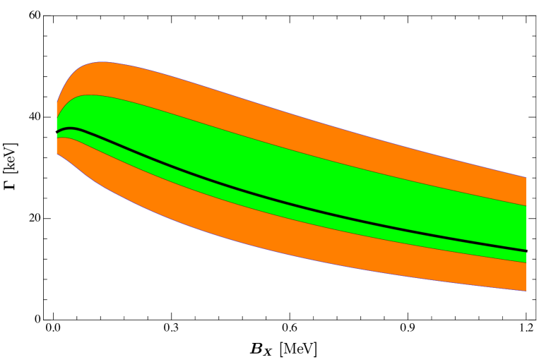
Figure 2: Partial decay rate of $X(3872)\to D^{0}\bar{D}^{0}\pi^{0}$ versus the binding energy $B_{X}$ of $X(3872)$. The central black solid line is the LO decay rate. The green band is the NLO correction that has already been obtained in Ref. Fleming et al. (2007). The orange band is the NLO correction coming from the two new interactions, i.e., $\pi^{0}D^{0}$ and $D^{0}\bar{D}^{0}$ rescattering.

In Fig. 2, we show NLO corrections to the partial decay rate of $X(3872)\to D^{0}\bar{D}^{0}\pi^{0}$. The green band reproduces the results already obtained in Ref. Fleming et al. (2007), where $\pi^{0}D^{0}$ and $D^{0}\bar{D}^{0}$ rescattering were not included. The orange band is the additional correction due to the $\pi^{0}D^{0}$ and $D^{0}\bar{D}^{0}$ rescattering terms in the Lagrangian. In Fig. 2, $C_{\pi}$ is set to be $4.1\pm 0.7$ GeV^-1 which is derived in Appendix B. Currently, little is known about $C_{0D}$. We choose to vary it between a natural range of $[-1,1]~{}{\rm fm}^{2}$ to estimate its impact on the results. In particular $C_{0D}=1~{}{\rm fm}^{2}$ corresponds to having a $D^{0}\bar{D}^{0}$ bound state near threshold with scattering length approximately equal to $a$ $\sim$ $-\frac{m_{D}C_{0D}}{4\pi}=-\frac{1}{262}~{}{\rm MeV}^{-1}$ Guo et al. (2014). All other parameters are set to be the same as those in Ref. Fleming et al. (2007). Note that $\bar{g}$ differs slightly from the value used in Ref. Fleming et al. (2007) to be consistent with the most recent measurement of the decay width for $\Gamma[D^{*+}]$ Tanabashi et al. (2018), which is the reason why the central line of Fig. 2 is slightly lower than that in Ref. Fleming et al. (2007)). The two new interactions give rise to a correction up to about $25\%$. Interestingly, $D^{0}\bar{D}^{0}$ rescattering contribution dominates that of the $\pi^{0}D^{0}$ rescattering whose correction to the LO decay rate is less than $1\%$. This is reminiscent of the results obtained in Ref. Fleming et al. (2007), where it is found that the contact interaction contribution dominates that from the pion exchange diagrams.

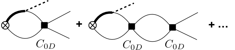
Figure 3: Resumming the $D^{0}\bar{D}^{0}$ rescattering diagram.

Figure 4: The NLO corrections from the $D^{0}\bar{D}^{0}$ rescattering diagram. Solid and dashed lines correspond to contributions from the $D^{0}\bar{D}^{0}$ rescattering diagrams without and with resummation shown in Fig. 3, respectively.

Since the $D^{0}\bar{D}^{0}$ rescattering gives a large NLO correction to the partial decay rate of $X(3872)\to D^{0}\bar{D}^{0}\pi^{0}$, it is interesting to see the resummation effect of final state rescattering as shown in Fig. 3. The resummation is equivalent to replacing $C_{0D}$ with the effective range expansion Kaplan et al. (1998b)

$$C_{0D}\to-\frac{4\pi}{m_{D}}\frac{1}{1/a+ip}$$ (9)

where $a$ is the $D^{0}\bar{D}^{0}$ scattering length (set to be $-\frac{1}{262}$ ${\rm MeV}^{-1}$ as mentioned above) and $p=|(\vec{p}_{D}-\vec{p}_{\bar{D}})/2|$. The correction from such a resummation is not significant, though, as is shown in Fig. 4, where the dashed line (from the resummed $D^{0}\bar{D}^{0}$ rescattering diagram) only gives a small modification to the solid line (from the $D^{0}\bar{D}^{0}$ rescattering diagram without resummation). Overall, the effect of resumming $D^{0}\bar{D}^{0}$ rescattering diagram shown in Fig. 3 contributes to less than $1\%$ correction to the LO partial decay rate of $X(3872)\to D^{0}\bar{D}^{0}\pi^{0}$.

Next we investigate the $\pi^{0}$ kinetic energy, $E_{\pi}$, distribution from $X(3872)$ decaying to $D^{0}\bar{D}^{0}\pi^{0}$. The analytic expression can be obtained readily from Eq. (III) by changing variable from $p_{\bar{D}}$ to $E_{\pi}$ using energy conservation in the $X(3872)$ rest frame

$$p_{\bar{D}}^{2}=2m_{D}\left(M_{X}-m_{\pi}-2m_{D}-E_{\pi}-\frac{p_{D}^{2}}{2m_{D}}\right),$$ (10)

which leads to

$$\frac{d\Gamma}{dE_{\pi}dp_{D}^{2}}=2m_{D}\frac{d\Gamma}{dp_{D}^{2}dp_{\bar{D}}^{2}}.$$ (11)

where the prefactor $2m_{D}$ on the right hand side comes from the Jacobian for changing variables, and $p_{\bar{D}}$ is expressed in terms of $E_{\pi}$ and $p_{D}$ using Eq. (10). Then the $\pi^{0}$ kinetic energy $E_{\pi}$ distribution is obtained by integrating over $p_{D}$.

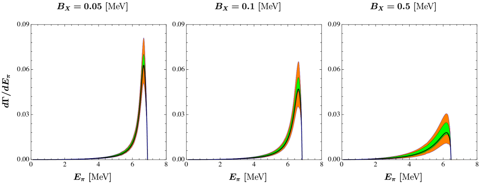
Figure 5: The $\pi^{0}$ kinetic energy distribution for the decay process $X(3872)\to D^{0}\bar{D}^{0}\pi^{0}$. Color and line conventions for the plots are the same as those used in Fig. 2.

Figure 6: Effects of the dynamics of $D^{0*}$ (and $\bar{D}^{0*}$) as indicated in the LO amplitude Eq. (2). The dashed curves are normalized to have the same areas as the solid curves in each panel respectively. The solid curves are the LO $E_{\pi}$ distribution from Eq. (2) and dashed curves are the LO $E_{\pi}$ distribution from Eq. (2) with the $D^{0*}$ (and $\bar{D}^{0*}$) propagators set to a constant.

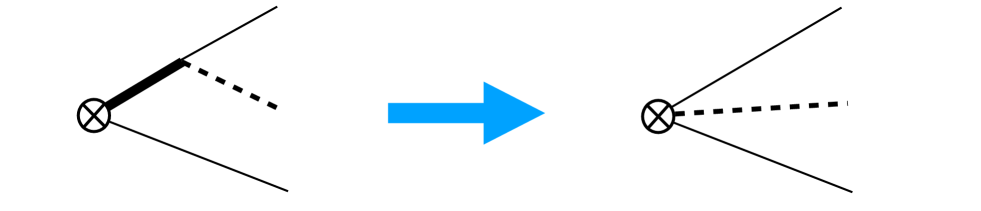
Figure 7: Shrinking of the $D^{0*}$ ($\bar{D}^{0*}$) propagators to contact interactions with $X(3872)$.

Figure 5 shows the $\pi^{0}$ kinetic energy, $E_{\pi}$, distributions for different binding energies, $B_{X}$, of $X(3872)$. As $B_{X}$ decreases, the location of the peaks shifts to higher energies and the peak is higher and more narrow. As shown in Fig. 2, the $D^{0}\bar{D}^{0}$ rescattering gives rise to large NLO corrections, which makes the extraction of $X(3872)$ binding energy from the partial decay rate difficult without further knowledge of the $D\bar{D}$ interaction (see also Ref. Guo et al. (2014)). Figure 5 shows, however, the location of the peak of the $E_{\pi}$ distribution is insensitive to NLO corrections, so it could be a better observable for extracting properties of $X(3872)$. While the three-body phase-space is important in determining the overall features of $E_{\pi}$ distributions, the sharpness of the peaks is due to the pole from the virtual $D^{0*}$ (and $\bar{D}^{0*}$) propagator, which is a consequence of the molecular nature of the $X(3872)$. To further illustrate this point, we do a simple LO analysis of $E_{\pi}$ distribution based on LO amplitude Eq. (2). In Fig. 6, the solid curves are the same as the LO curves shown in Fig. 5 and dashed curves are LO $E_{\pi}$ distribution obtained by setting the $D^{0*}$ (and $\bar{D}^{0*}$) propagators in Eq. (2) to a constant which effectively shrinks the propagators to contact interactions with $X(3872)$ as shown in Fig. 7. Thus the dashed curves come from pure three-body phase-space ($\times p_{\pi}^{2}$), while for the solid curves the location and width of peaks have genuine information about the $D^{0*}$ (and $\bar{D}^{0*}$) binding in the $X(3872)$.

IV Conclusions

In this paper we revisited the XEFT calculation of $X(3872)\to D^{0}\bar{D}^{0}\pi^{0}$ first performed in Ref. Fleming et al. (2007). We included corrections from the $\pi^{0}D^{0}$, $\pi^{0}\bar{D}^{0}$ and $D^{0}\bar{D}^{0}$ rescattering. The $D^{0}\bar{D}^{0}$ rescattering is by far the most important. The total uncertainty in the partial width is of order $50\%$ and the $D^{0}\bar{D}^{0}$ rescattering accounts for about half. We also calculate the differential distribution in the pion energy. This turns out to be quite interesting. Because of poles in diagrams with virtual $D^{*0}(\bar{D}^{*0})$ mesons, the distribution is highly peaked near maximal pion energy. The shape of this distribution is sensitive to the binding energy of the $X(3872)$. As the binding energy approaches zero, the location of the peak shifts upwards and the peak becomes narrower and higher. Unlike the partial width, the shape of the distribution and the location of the peak are insensitive to higher order corrections. It would be very interesting to make an experimental measurement of this distribution, in particular before the proposal of measuring the $X(3872)$ binding energy using triangle singularity Guo (2019) is realized experimentally.

Appendix A Loop integrals

Here we define the loop integrals involved in the calculations. We choose to work in the rest frame of the decay particle, $P^{\mu}=(M,\vec{0})$. The basic scalar 3-point loop integral is UV convergent, and can be worked out as Guo et al. (2011)

$$I(q) = i\int\!\frac{d^{d}l}{(2\pi)^{d}}\frac{1}{\left(l^{0}-\frac{\vec{l}\ ^{2}}{2m_{1}}+i\epsilon\right)\left(-b_{12}-l^{0}-\frac{\vec{l}\ ^{2}}{2m_{2}}+i\epsilon\right)\left[l^{0}+b_{12}-b_{23}-\frac{(\vec{l}-\vec{q})^{2}}{2m_{3}}+i\epsilon\right]}$$ (A.1)

$$= 4\mu_{12}\mu_{23}\int\!\frac{d^{d-1}l}{(2\pi)^{d-1}}\frac{1}{\left(\vec{l}\ ^{2}+c_{1}-i\epsilon\right)\left(\vec{l}\ ^{2}-\frac{2\mu_{23}}{m_{3}}\vec{l}\cdot\vec{q}+c_{2}-i\epsilon\right)}$$

$$= 4\mu_{12}\mu_{23}\int_{0}^{1}dx\int\!\frac{d^{d-1}l}{(2\pi)^{d-1}}\frac{1}{\left[\vec{l}\ ^{2}-ax^{2}+(c_{2}-c_{1})x+c_{1}-i\epsilon\right]^{2}}$$

$$= \frac{4\mu_{12}\mu_{23}}{(4\pi)^{(d-1)/2}}\Gamma\left(\frac{5-d}{2}\right)\int_{0}^{1}dx\left[-ax^{2}+(c_{2}-c_{1})x+c_{1}-i\epsilon\right]^{(d-5)/2}$$

$$= \frac{\mu_{12}\mu_{23}}{2\pi}\frac{1}{\sqrt{a}}\left[\tan^{-1}\left(\frac{c_{2}-c_{1}}{2\sqrt{ac_{1}}}\right)+\tan^{-1}\left(\frac{2a+c_{1}-c_{2}}{2\sqrt{a(c_{2}-a)}}\right)\right],$$

where $\mu_{ij}=m_{i}m_{j}/(m_{i}+m_{j})$ are the reduced masses, $b_{12}=m_{1}+m_{2}-M$, $b_{23}=m_{2}+m_{3}+q^{0}-M$, and

$$a=\left(\frac{\mu_{23}}{m_{3}}\right)^{2}\vec{q}\ ^{2},\quad c_{1}=2\mu_{12}b_{12},\quad c_{2}=2\mu_{23}b_{23}+\frac{\mu_{23}}{m_{3}}\vec{q}\ ^{2}.$$ (A.2)

There is no pole for $d\leq 4$, and we have taken $d=4$ in the last step.

We also need the vector and tensor loop integrals which are defined as

$$q^{i}I^{(1)}(q)\equiv i\int\!\frac{d^{d}l}{(2\pi)^{d}}l^{i}\times[\text{integrand of }I(q)],$$ (A.3)

and

$$q^{i}q^{j}I^{(2)}_{0}(q)+\delta^{ij}\vec{q}\ ^{2}I^{(2)}_{1}(q)\equiv i\int\!\frac{d^{d}l}{(2\pi)^{d}}{l^{i}l^{j}}\times[\text{integrand of }I(q)].$$ (A.4)

They can be expressed in terms of the scalar 2-point and 3-point loop integrals as

$$I^{(1)}(q) = \frac{\mu_{23}}{am_{3}}\left[B(c_{2}-a)-B(c_{1})+\frac{1}{2}(c_{2}-c_{1})I(q)\right],$$ (A.5)

$$\vec{q}\ ^{2}I^{(2)}_{0}(q) = \frac{d-3}{d-2}B(c_{2}-a)+\frac{c_{1}}{d-2}I(q)+\frac{d-1}{d-2}(c_{2}-c_{1})\frac{m_{3}}{2\mu_{23}}I^{(1)}(q),$$ (A.6)

$$\vec{q}\ ^{2}I^{(2)}_{1}(q) = \frac{1}{d-2}B(c_{2}-a)-\frac{c_{1}}{d-2}I(q)-\frac{1}{d-2}(c_{2}-c_{1})\frac{m_{3}}{2\mu_{23}}I^{(1)}(q),$$ (A.7)

where the function $B(c)=2\mu_{12}\mu_{23}\Sigma(c)$ with $\Sigma(c)$ defined as (in the PDS scheme)

$$\Sigma(c) \equiv \left(\frac{\Lambda_{\rm PDS}}{2}\right)^{4-d}\!\int\!\frac{d^{d-1}l}{(2\pi)^{d-1}}\frac{1}{\vec{l}\ ^{2}+c-i\epsilon}$$ (A.8)

$$= \left(\frac{\Lambda_{\rm PDS}}{2}\right)^{4-d}(4\pi)^{(1-d)/2}\Gamma\left(\frac{3-d}{2}\right)(c-i\epsilon)^{(d-3)/2}$$

$$= \frac{1}{4\pi}\left(\Lambda_{\rm PDS}-\sqrt{c-i\epsilon}\right).$$

Notice that although the expression for $I^{(2)}_{0}(q)$ contains the $B$ function, it is in fact UV convergent since $l^{i}l^{j}$ in Eq. (A.4) is converted to $q^{i}q^{j}$, a factor of the external momentum, for this term. The $(d-3)$ factor in front of the $B$ function in Eq. (A.6) cancels the $1/(d-3)$ pole term in the $B$ function.

Appendix B ${D\pi}$ scattering length

In this appendix, the numerical value of $C_{\pi}$ used in our plots is derived. We use the isospin phase convention:

$${\left|\pi^{+}\right\rangle}=-{\left|1,+1\right\rangle},\qquad{\left|D^{+}\right\rangle}=-{\left|\frac{1}{2},+\frac{1}{2}\right\rangle},$$ (B.9)

while all the other $D$ and pion fields take the positive sign. With this convention, the $D^{0}\pi^{0}$ is expressed in terms of isospin eigenstates as

$${\left|D^{0}\pi^{0}\right\rangle}=\sqrt{\frac{2}{3}}\,{\left|\frac{3}{2},-\frac{1}{2}\right\rangle}+\frac{1}{\sqrt{3}}\,{\left|\frac{1}{2},-\frac{1}{2}\right\rangle}.$$ (B.10)

Then the $D^{0}\pi^{0}\to D^{0}\pi^{0}$ scattering length receives contributions from both isospin $I=1/2$ and $I=3/2$ channels as

$$a_{D^{0}\pi^{0}}=\frac{2}{3}a_{D\pi}^{3/2}+\frac{1}{3}a_{D\pi}^{1/2}=(0.06\pm 0.01)~{}\text{fm},$$ (B.11)

where we have used $a_{D\pi}^{1/2}=0.37^{+0.03}_{-0.02}$ fm and $a_{D\pi}^{3/2}=-(0.100\pm 0.002)$ fm from Ref. Liu et al. (2013).

Then the dimensionless scattering amplitude at threshold with the relativistic normalization is

$$\mathcal{A}_{D^{0}\pi^{0}}(\sqrt{s}=M_{D^{0}}+M_{\pi^{0}})=8\pi(M_{D^{0}}+M_{\pi^{0}})a_{D^{0}\pi^{0}}.$$ (B.12)

Matching the above expression to $2M_{D^{0}}2M_{\pi^{0}}C_{\pi}/(2M_{\pi^{0}})$ gives

$$C_{\pi}=4\pi\left(1+\frac{M_{\pi^{0}}}{M_{D^{0}}}\right)a_{D^{0}\pi^{0}}=(4.1\pm 0.7)\,{\rm GeV}^{-1}.$$ (B.13)

References

- Abe et al. (2003) Kazuo Abe et al. (Belle), “Observation of a new narrow charmonium state in decays,” in Proceedings, 21st International Symposium on Lepton and Photon Interactions at High Energies (LP 03): Batavia, ILL, August 11-16, 2003 (2003) arXiv:hep-ex/0308029 [hep-ex] .
- Chen et al. (2016) Hua-Xing Chen, Wei Chen, Xiang Liu, and Shi-Lin Zhu, “The hidden-charm pentaquark and tetraquark states,” Phys. Rept. 639, 1–121 (2016), arXiv:1601.02092 [hep-ph] .
- Richard (2016) Jean-Marc Richard, “Exotic hadrons: review and perspectives,” Few Body Syst. 57, 1185–1212 (2016), arXiv:1606.08593 [hep-ph] .
- Esposito et al. (2016) A. Esposito, A. Pilloni, and A. D. Polosa, “Multiquark Resonances,” Phys. Rept. 668, 1–97 (2016), arXiv:1611.07920 [hep-ph] .
- Hosaka et al. (2016) Atsushi Hosaka, Toru Iijima, Kenkichi Miyabayashi, Yoshihide Sakai, and Shigehiro Yasui, “Exotic hadrons with heavy flavors: X, Y, Z, and related states,” PTEP 2016, 062C01 (2016), arXiv:1603.09229 [hep-ph] .
- Lebed et al. (2017) Richard F. Lebed, Ryan E. Mitchell, and Eric S. Swanson, “Heavy-Quark QCD Exotica,” Prog. Part. Nucl. Phys. 93, 143–194 (2017), arXiv:1610.04528 [hep-ph] .
- Guo et al. (2018) Feng-Kun Guo, Christoph Hanhart, Ulf-G. Meißner, Qian Wang, Qiang Zhao, and Bing-Song Zou, “Hadronic molecules,” Rev. Mod. Phys. 90, 015004 (2018), arXiv:1705.00141 [hep-ph] .
- Ali et al. (2017) Ahmed Ali, Jens Sören Lange, and Sheldon Stone, “Exotics: Heavy Pentaquarks and Tetraquarks,” Prog. Part. Nucl. Phys. 97, 123–198 (2017), arXiv:1706.00610 [hep-ph] .
- Olsen et al. (2018) Stephen Lars Olsen, Tomasz Skwarnicki, and Daria Zieminska, “Nonstandard heavy mesons and baryons: Experimental evidence,” Rev. Mod. Phys. 90, 015003 (2018), arXiv:1708.04012 [hep-ph] .
- Kou et al. (2018) E. Kou, P. Urquijo, W. Altmannshofer, et al. (Belle-II), “The Belle II Physics Book,” (2018), arXiv:1808.10567 [hep-ex] .
- Cerri et al. (2018) A. Cerri et al., “Opportunities in Flavour Physics at the HL-LHC and HE-LHC,” (2018), arXiv:1812.07638 [hep-ph] .
- Liu et al. (2019) Yan-Rui Liu, Hua-Xing Chen, Wei Chen, Xiang Liu, and Shi-Lin Zhu, “Pentaquark and Tetraquark states,” Prog. Part. Nucl. Phys. 107, 237–320 (2019), arXiv:1903.11976 [hep-ph] .
- Brambilla et al. (2019) Nora Brambilla, Simon Eidelman, Christoph Hanhart, Alexey Nefediev, Cheng-Ping Shen, Christopher E. Thomas, Antonio Vairo, and Chang-Zheng Yuan, “The states: experimental and theoretical status and perspectives,” (2019), arXiv:1907.07583 [hep-ex] .
- Kalashnikova and Nefediev (2019) Yu S. Kalashnikova and A. V. Nefediev, “X(3872) in the molecular model,” Phys. Usp. 62, 568–595 (2019), [Usp. Fiz. Nauk189,no.6,603(2019)], arXiv:1811.01324 [hep-ph] .
- Aaij et al. (2013) R Aaij et al. (LHCb), “Determination of the X(3872) meson quantum numbers,” Phys. Rev. Lett. 110, 222001 (2013), arXiv:1302.6269 [hep-ex] .
- Tanabashi et al. (2018) M. Tanabashi et al. (Particle Data Group), “Review of Particle Physics,” Phys. Rev. D98, 030001 (2018).
- Voloshin (2004) M. B. Voloshin, “Interference and binding effects in decays of possible molecular component of ,” Phys. Lett. B579, 316–320 (2004), arXiv:hep-ph/0309307 [hep-ph] .
- Mehen (2015) Thomas Mehen, “Hadronic loops versus factorization in effective field theory calculations of ,” Phys. Rev. D92, 034019 (2015), arXiv:1503.02719 [hep-ph] .
- Li and Yuan (2019) Chunhua Li and Chang-Zheng Yuan, “Determination of the absolute branching fractions of decays,” Phys. Rev. D100, 094003 (2019), arXiv:1907.09149 [hep-ex] .
- Braaten et al. (2019) Eric Braaten, Li-Ping He, and Kevin Ingles, “Branching Fractions of the ,” (2019), arXiv:1908.02807 [hep-ph] .
- Fleming et al. (2007) S. Fleming, M. Kusunoki, T. Mehen, and U. van Kolck, “Pion interactions in the ,” Phys. Rev. D76, 034006 (2007), arXiv:hep-ph/0703168 [hep-ph] .
- Fleming and Mehen (2008) Sean Fleming and Thomas Mehen, “Hadronic Decays of the to in Effective Field Theory,” Phys. Rev. D78, 094019 (2008), arXiv:0807.2674 [hep-ph] .
- Fleming and Mehen (2012) Sean Fleming and Thomas Mehen, “The decay of the into and the Operator Product Expansion in XEFT,” Phys. Rev. D85, 014016 (2012), arXiv:1110.0265 [hep-ph] .
- Mehen and Springer (2011) Thomas Mehen and Roxanne Springer, “Radiative Decays and in Effective Field Theory,” Phys. Rev. D83, 094009 (2011), arXiv:1101.5175 [hep-ph] .
- Margaryan and Springer (2013) Arman Margaryan and Roxanne P. Springer, “Using the decay to probe the molecular content of the ,” Phys. Rev. D88, 014017 (2013), arXiv:1304.8101 [hep-ph] .
- Braaten et al. (2010) Eric Braaten, H.-W. Hammer, and Thomas Mehen, “Scattering of an Ultrasoft Pion and the ,” Phys. Rev. D82, 034018 (2010), arXiv:1005.1688 [hep-ph] .
- Canham et al. (2009) David L. Canham, H.-W. Hammer, and Roxanne P. Springer, “On the scattering of and mesons off the ,” Phys. Rev. D80, 014009 (2009), arXiv:0906.1263 [hep-ph] .
- Jansen et al. (2014) M. Jansen, H.-W. Hammer, and Yu Jia, “Light quark mass dependence of the in an effective field theory,” Phys. Rev. D89, 014033 (2014), arXiv:1310.6937 [hep-ph] .
- Jansen et al. (2015) M. Jansen, H.-W. Hammer, and Yu Jia, “Finite volume corrections to the binding energy of the ,” Phys. Rev. D92, 114031 (2015), arXiv:1505.04099 [hep-ph] .
- Alhakami and Birse (2015) Mohammad H. Alhakami and Michael C. Birse, “Power counting for three-body decays of a near-threshold state,” Phys. Rev. D91, 054019 (2015), arXiv:1501.06750 [hep-ph] .
- Braaten (2015) Eric Braaten, “Galilean-invariant effective field theory for the ,” Phys. Rev. D91, 114007 (2015), arXiv:1503.04791 [hep-ph] .
- AlFiky et al. (2006) Mohammad T. AlFiky, Fabrizio Gabbiani, and Alexey A. Petrov, “: Hadronic molecules in effective field theory,” Phys. Lett. B640, 238–245 (2006), arXiv:hep-ph/0506141 [hep-ph] .
- Baru et al. (2011) V. Baru, A. A. Filin, C. Hanhart, Yu. S. Kalashnikova, A. E. Kudryavtsev, and A. V. Nefediev, “Three-body dynamics for the ,” Phys. Rev. D84, 074029 (2011), arXiv:1108.5644 [hep-ph] .
- Valderrama (2012) M. Pavon Valderrama, “Power Counting and Perturbative One Pion Exchange in Heavy Meson Molecules,” Phys. Rev. D85, 114037 (2012), arXiv:1204.2400 [hep-ph] .
- Nieves and Valderrama (2012) J. Nieves and M. Pavon Valderrama, “The Heavy Quark Spin Symmetry Partners of the X(3872),” Phys. Rev. D86, 056004 (2012), arXiv:1204.2790 [hep-ph] .
- Baru et al. (2013) V. Baru, E. Epelbaum, A. A. Filin, C. Hanhart, U. G. Meissner, and A. V. Nefediev, “Quark mass dependence of the binding energy,” Phys. Lett. B726, 537–543 (2013), arXiv:1306.4108 [hep-ph] .
- Guo et al. (2013a) Feng-Kun Guo, Christoph Hanhart, Ulf-G. Meißner, Qian Wang, and Qiang Zhao, “Production of the in charmonia radiative decays,” Phys. Lett. B725, 127–133 (2013a), arXiv:1306.3096 [hep-ph] .
- Guo et al. (2013b) Feng-Kun Guo, Carlos Hidalgo-Duque, Juan Nieves, and Manuel Pavon Valderrama, “Consequences of Heavy Quark Symmetries for Hadronic Molecules,” Phys. Rev. D88, 054007 (2013b), arXiv:1303.6608 [hep-ph] .
- Baru et al. (2015) V. Baru, E. Epelbaum, A. A. Filin, F.-K. Guo, H.-W. Hammer, C. Hanhart, U.-G. Meißner, and A. V. Nefediev, “Remarks on study of from effective field theory with pion-exchange interaction,” Phys. Rev. D91, 034002 (2015), arXiv:1501.02924 [hep-ph] .
- Schmidt et al. (2018) M. Schmidt, M. Jansen, and H. W Hammer, “Threshold Effects and the Line Shape of the X(3872) in Effective Field Theory,” Phys. Rev. D98, 014032 (2018), arXiv:1804.00375 [hep-ph] .
- Guo et al. (2008) Feng-Kun Guo, Christoph Hanhart, Siegfried Krewald, and Ulf-G. Meißner, “Subleading contributions to the width of the ,” Phys. Lett. B666, 251–255 (2008), arXiv:0806.3374 [hep-ph] .
- Guo et al. (2009) Feng-Kun Guo, Christoph Hanhart, and Ulf-G. Meißner, “Interactions between heavy mesons and Goldstone bosons from chiral dynamics,” Eur. Phys. J. A40, 171–179 (2009), arXiv:0901.1597 [hep-ph] .
- Liu et al. (2013) Liuming Liu, Kostas Orginos, Feng-Kun Guo, Christoph Hanhart, and Ulf-G. Meißner, “Interactions of charmed mesons with light pseudoscalar mesons from lattice QCD and implications on the nature of the ,” Phys. Rev. D87, 014508 (2013), arXiv:1208.4535 [hep-lat] .
- Mohler et al. (2013) Daniel Mohler, Sasa Prelovsek, and R. M. Woloshyn, “ scattering and meson resonances from lattice QCD,” Phys. Rev. D87, 034501 (2013), arXiv:1208.4059 [hep-lat] .
- Guo et al. (2019) Zhi-Hui Guo, Liuming Liu, Ulf-G Meißner, J. A. Oller, and A. Rusetsky, “Towards a precise determination of the scattering amplitudes of the charmed and light-flavor pseudoscalar mesons,” Eur. Phys. J. C79, 13 (2019), arXiv:1811.05585 [hep-ph] .
- Guo et al. (2014) F.-K. Guo, C. Hidalgo-Duque, J. Nieves, Altug Ozpineci, and M. P. Valderrama, “Detecting the long-distance structure of the (3872),” Eur. Phys. J. C74, 2885 (2014), arXiv:1404.1776 [hep-ph] .
- Wise (1992) Mark B. Wise, “Chiral perturbation theory for hadrons containing a heavy quark,” Phys. Rev. D45, R2188 (1992).
- Burdman and Donoghue (1992) Gustavo Burdman and John F. Donoghue, “Union of chiral and heavy quark symmetries,” Phys. Lett. B280, 287–291 (1992).
- Yan et al. (1992) Tung-Mow Yan, Hai-Yang Cheng, Chi-Yee Cheung, Guey-Lin Lin, Y. C. Lin, and Hoi-Lai Yu, “Heavy quark symmetry and chiral dynamics,” Phys. Rev. D46, 1148–1164 (1992), [Erratum: Phys. Rev.D55,5851(1997)].
- Kaplan et al. (1998a) David B. Kaplan, Martin J. Savage, and Mark B. Wise, “A New expansion for nucleon-nucleon interactions,” Phys. Lett. B424, 390–396 (1998a), arXiv:nucl-th/9801034 [nucl-th] .
- Kaplan et al. (1998b) David B. Kaplan, Martin J. Savage, and Mark B. Wise, “Two nucleon systems from effective field theory,” Nucl. Phys. B534, 329–355 (1998b), arXiv:nucl-th/9802075 [nucl-th] .
- Mehen and Powell (2011) Thomas Mehen and Joshua W. Powell, “Heavy Quark Symmetry Predictions for Weakly Bound B-Meson Molecules,” Phys. Rev. D84, 114013 (2011), arXiv:1109.3479 [hep-ph] .
- Mehen and Powell (2013) Thomas Mehen and Josh Powell, “Line shapes in with and using effective field theory,” Phys. Rev. D88, 034017 (2013), arXiv:1306.5459 [hep-ph] .
- Wilbring et al. (2013) E. Wilbring, H.-W. Hammer, and U.-G. Meißner, “Electromagnetic Structure of the ,” Phys. Lett. B726, 326–329 (2013), arXiv:1304.2882 [hep-ph] .
- Guo (2019) Feng-Kun Guo, “Novel Method for Precisely Measuring the Mass,” Phys. Rev. Lett. 122, 202002 (2019), arXiv:1902.11221 [hep-ph] .
- Guo et al. (2011) Feng-Kun Guo, Christoph Hanhart, Gang Li, Ulf-G. Meißner, and Qiang Zhao, “Effect of charmed meson loops on charmonium transitions,” Phys. Rev. D83, 034013 (2011), arXiv:1008.3632 [hep-ph] .