Galactic Archaeology with asteroseismic ages. II.
Confirmation of a delayed gas infall using Bayesian
analysis based on MCMC methods

Abstract

Context. With the wealth of information from large surveys and observational campaigns in the contemporary era, it is critical to properly exploit the data to constrain the parameters of Galactic chemical evolution models and quantify the associated uncertainties.

Aims. We aim at constraining the two-infall chemical evolution models for the solar annulus using the measured chemical abundance ratios and seismically inferred age of stars in the APOKASC sample. In the revised two-infall chemical evolution models by Spitoni et al. (2019b), a significant delay of $\sim 4.3$ Gyr has been invoked between the two episodes of gas accretion. In this work, we wish to test its robustness and statistically confirm/quantify the delay.

Methods. For the first time, a Bayesian framework based on Markov Chain Monte Carlo methods has been used for fitting the two-infall chemical evolution models to the data.

Results. In addition to fitting the data for stars in the APOKASC sample, our best fit models also reproduce other important observational constraints of the chemical evolution of the disk: i) present day stellar surface density; ii) present-day supernova and star formation rates; iii) the metallicity distribution function; and iv) solar abundance values. We found a significant delay between the two gas accretion episodes for various models explored with different values for the star formation efficiencies. The values for the delay lie in the range $4.5-5.5$ Gyr.

Conclusions. The results suggest that the APOKASC sample carries the signature of delayed gas-rich merger, with the dilution as main process determining the shape of low-$\alpha$ stars in the abundance ratios space.

1 Introduction

The purpose of Galactic Archaeology is to unveil the formation and evolution of our Galaxy by interpreting signatures imprinted in the observed chemical abundances and kinematics of resolved stellar populations. This is typically done through the proper exploitation of the observational stellar data to constrain models of Galactic chemical evolution. The contemporary wealth of data from big surveys and observational campaigns, e.g. spectroscopic properties from the Apache Point Observatory Galactic Evolution Experiment project (APOGEE; Majewski et al., 2017), kinematic properties from the ‘fossil’ record of old stellar populations as provided by the Gaia mission (DR2; Gaia Collaboration et al., 2018), and precise seismic ages from the Kepler satellite (Borucki et al., 2009), offer an unprecedented opportunity to test models of galaxy formation and evolution.

The analysis of the APOGEE data (Nidever et al., 2014; Hayden et al., 2015) suggested the existence of a clear distinction between two sequences of disc stars in the [$\alpha$/Fe] versus [Fe/H] abundance ratio space: the so-called high-$\alpha$ and low-$\alpha$ sequences. This dichotomy has been also confirmed by the Gaia-ESO survey (e.g., Recio-Blanco et al., 2014; Rojas-Arriagada et al., 2016, 2017) and the AMBRE project (Mikolaitis et al., 2017).

In several theoretical models of the Galactic discs evolution it has been proposed that this bimodality is strictly connected to a delayed gas accretion episode of primordial composition. For instance, a late second accretion phase after a prolonged period with a quenched star formation rate (SFR) has been suggested by the dynamical models presented by Noguchi (2018). Moreover, the AURIGA simulations presented by Grand et al. (2018) clearly point out that a bimodal distribution in the [Fe/H]-[$\alpha$/Fe] plane is a consequence of a significantly lowered gas accretion rate at ages between 6 and 9 Gyr. In the framework of cosmological hydrodynamic simulations of Milky Way like galaxies, Buck (2020) stated that a bimodal $\alpha$-sequence is a generic consequence of a gas-rich merger at some time in galaxy’s evolution. As also suggested by Spitoni et al. (2019b), the merger gives rise to the low-$\alpha$ sequence by bringing pristine metal-poor gas in the system which dilutes the metallicity of interstellar medium while keeping [$\alpha$/Fe] abundance almost unchanged (as first proposed in a cosmological model by Calura & Menci 2009).

The model presented by Spitoni et al. (2019b) (hereafter ES19) also includes precise stellar ages provided by asteroseismology to constrain the chemical evolution of the solar neighbourhood. The ES19 model is an updated version of the classical ”two-infall” of Chiappini et al. (1997), in which an early fast gas accretion episode gives rise to the high-$\alpha$ sequence, and at a later Galactic time, the low-$\alpha$ sequence is created by a different infall event characterized by a longer time-scale of accretion. The predictions of the revised “two-infall” models were compared with the measured chemical abundance ratios (Pinsonneault et al., 2014) and seismically inferred age of stars in the APOKASC catalogue (APOGEE + Kepler Asteroseismology Science Consortium; Silva Aguirre et al., 2018). ES19 model was capable of reproducing the APOKASC data assuming a disc component dissection based on chemistry (see Silva Aguirre et al., 2018), i.e. the sample was divided in two distinct groups called ‘high-$\alpha$’ and ‘low-$\alpha$’ sequences. The most important result of ES19 was that a significant delay of $\sim$ 4.3 Gyr between the two infall episodes was required to reproduce the measured stellar abundances and seismically inferred ages.

In ES19 the choice of free parameters, i.e. the two infall time scales, the corresponding star formation efficiencies and the delay between the two infall episodes of the model was made to qualitatively reproduce the observed [$\alpha$/Fe] versus [Fe/H] abundance ratios. In this article we present a quantitative study of the free parameters using a Bayesian analysis. Probabilistic data analysis has transformed scientific research in the past decade. In particular, Bayesian analysis based on Markov Chain Monte Carlo (MCMC) methods have been used in several different areas of astrophysics including cosmology (Dunkley et al. 2005), cosmic rays (Putze et al. 2010), active galactic nuclei (Reynolds et al. 2012), Milky Way dwarf satellites (Ural et al. 2015), semi-analytical models of galaxy formation (Kampakoglou et al. 2008; Henriques et al. 2009, 2013), and stellar nucleosynthesis (Cescutti et al. 2018), among other. Recently, MCMC methods have been used in testing Galactic chemical evolution models (see e.g. Côté et al., 2017; Rybizki et al., 2017; Philcox et al., 2018; Frankel et al., 2018; Belfiore et al., 2019).

In this paper, we present the first attempt to perform a detailed study of the key parameters which regulate the evolution of the solar neighbourhood by means of a match between a Bayesian MCMC method and the two-infall chemical evolution model. The goal is to test the findings of ES19 by quantitatively inferring the delay between the two accretion episodes without imposing any stellar data separation based on chemical abundances.

The paper is organised as follows: in Section 2 the observational data used in the Bayesian analysis is presented, in Section 3 we briefly recall the main characteristics of two infall model, in Section 4 we describe the fitting method and also perform a preliminary test, in Section 5 we present our results, and finally in Section 6 we summarize our conclusions.

2 The APOKASC sample

In this work we use a Bayesian framework based on MCMC methods to fit state-of-the-art models of Galactic chemical evolution to the observed chemical abundance ratios and asteroseismic ages of stars in the updated APOKASC (APOGEE+ Kepler Asteroseismology Science Consortium) sample presented by Silva Aguirre et al. (2018).

The sample is composed by 1197 red giants spanning out to 2 kpc in the solar annulus with stellar properties determined combining the photometric, spectroscopic, and asteroseismic observables in the BAyesian STellar Algorithm (BASTA, Silva Aguirre et al., 2015, 2017) framework. The sample is also characterized by precise kinematic information available from the first DR of Gaia (Lindegren et al., 2016; Gaia Collaboration et al., 2016) and The Fourth US Naval Observatory CCD Astrograph (UCAC-4) catalogue (Zacharias et al., 2013). Here, it is assumed that $\alpha$ abundances are given by the sum of the individual Mg and Si abundances (Salaris et al., 2018).

As in ES19, in the present work we do not consider the so-called “young $\alpha$ rich” (Y$\alpha$R) stars. The origin of these stars is still uncertain and two different scenarios have been proposed: either they are objects migrated from the Galactic bar Chiappini et al. (2015) or evolved blue stragglers (Martig et al., 2015; Chiappini et al., 2015; Yong et al., 2016; Jofré et al., 2016).

3 The revised two-infall model by ES19

In this Section we recall the main assumptions and characteristics of the revised two-infall chemical evolution model proposed by ES19. A few details on the model are provided, including the parametrization of the most basic physical processes (e. g. infall and star formation), as well as the stellar nucleosynthesis prescriptions used in the work.

3.1 The chemical evolution model prescriptions

In ES19 the authors revised the classical “two-infall” chemical evolution model in order to reproduce the data from updated APOKASC catalogue by Silva Aguirre et al. (2018) which were chemically dissected in high-$\alpha$ and low-$\alpha$ stellar sequences. From the precise stellar ages determined via asteroseismology, a clear age difference emerged in the solar annulus between high-$\alpha$ and low-$\alpha$ stars. The low-$\alpha$ sequence age distribution peaks at $\sim$ 2 Gyr, whereas the high-$\alpha$ one does so at $\sim$ 11 Gyr.

In ES19 the Milky Way disc is assumed to be formed by two distinct accretion episodes of gas. The gas infall rate is expressed by the following expression,

$$\mathcal{I}_{i}(t,i)=(\mathcal{X}_{i})_{inf}\left[\mathcal{N}_{1}\,e^{-t/\tau_{1}}+\theta(t-t_{{\rm max}})\mathcal{N}_{2}\,e^{-(t-t_{{\rm max}})/\tau_{2}}\right],$$ (1)

where $\tau_{1}$ is the time-scale for the formation of the high-$\alpha$ sequence which was fixed at a value of 0.1 Gyr and $\tau_{2}$ is the time-scale for the formation of the low-$\alpha$ disc phase which was fixed at a value of 8 Gyr. We remind the reader that the $\theta$ in the equation above is the Heaviside step function. $(\mathcal{X}_{i})_{inf}$ is the abundance by mass of the element $i$ in the infalling gas which is assumed to have primordial composition, whereas $t_{{\rm max}}$=4.3 Gyr is the time of the maximum infall rate on the second accretion episode, i.e. it indicates the delay of the beginning of the second infall. ES19 emphasised the importance of the $t_{{\rm max}}$ value in order to properly reproduce the APOKASC data. Finally, the coefficients $\mathcal{N}_{1}$ and $\mathcal{N}_{2}$ are obtained by imposing a fit to the observed current total surface mass density in the solar neighbourhood adopting the relations

$$\mathcal{N}_{1}=\frac{\sigma_{1}}{\tau_{1}\left(1-e^{-t_{G}/\tau_{1}}\right)},$$ (2)

$$\mathcal{N}_{2}=\frac{\sigma_{2}}{\tau_{2}\left(1-e^{-(t_{G}-t_{{\rm max}})/\tau_{2}}\right)},$$ (3)

where $\sigma_{1}$ and $\sigma_{2}$ are the present day total surface mass density of the high-$\alpha$ and low-$\alpha$ sequence stars, respectively; $t_{G}$ is the Age of the Milky Way.

The star formation rate is expressed as the Kennicutt (1998) law,

$$\psi(t)=\nu\sigma_{g}^{k}(t),$$ (4)

where $\nu$ is the star formation efficiency (SFE), $\sigma_{g}$ is the surface gas density, and $k=1.5$ is the exponent. In ES19 the adopted SFE is constant during the whole Galactic life and fixed at the value of $\nu=1.3$ Gyr^-1. However, different infall episodes could in principle be characterized by different SFEs. In fact, in the two-infall model by Grisoni et al. (2017, 2018) the SFEs associated to the high and low $\alpha$ sequences are different: $\nu_{1}=2$ Gyr^-1 and $\nu_{2}=1$ Gyr^-1.

We adopt the Scalo (1986) initial stellar mass function (IMF), constant in time and space.

3.2 Nucleosynthesis prescriptions and solar values

As for the nucleosynthesis prescriptions for Fe, Mg and Si, ES19 adopted the ones suggested by François et al. (2004). For a detailed description we refer to ES19. This set of yields has been widely used in the literature (Cescutti et al., 2007; Spitoni & Matteucci, 2011; Mott et al., 2013; Spitoni et al., 2015, 2017, 2019a; Vincenzo et al., 2019) and turned out to be able to reproduce the main features of the solar neighbourhood.

We have adopted the photospheric values of Asplund et al. (2005) as our solar reference abundances to be consistent with the APOGEE data release (García Pérez et al., 2016).

4 The fitting method

Bayesian analysis based on MCMC methods has transformed scientific research in the past decade. Since there are already several text books and reviews on Bayesian statistics (see e.g. Jaynes, 2003; Gelman et al., 2013) and MCMC methods (see e.g. Brooks et al., 2011; Sharma, 2017; Hogg & Foreman-Mackey, 2018; Speagle, 2019), we only describe them briefly and highlight the aspects specific to the problem at hand.

In the context of parameter estimation, Bayes’ theorem provides a way to update the parameters based on any new available data. In other words, it enables the calculation of the posterior probability distribution of the parameters given the new data,

$$P({\bf\Theta}|{\bf x})=\frac{P({\bf\Theta})}{P({\bf x})}P({\bf x}|{\bf\Theta}),$$ (5)

where ${\bf x}$ represents the set of observables, ${\bf\Theta}$ the set of model parameters, $P({\bf x}|{\bf\Theta})\equiv\mathscr{L}$ the likelihood (i.e. probability of observing the data given the model parameters), $P({\bf\Theta})$ the prior (i.e. probability of the model parameters before seeing the data, ${\bf x}$), and $P({\bf x})$ represents the evidence (i.e. total probability of observing the data). The evidence is a normalizing constant and can be calculated by integrating the likelihood over all model parameters. In the current study, ${\bf x}=\{[\alpha/{\rm Fe}],\ [{\rm Fe}/{\rm H}],\ {\rm age}\}$ and ${\bf\Theta}=\{\tau_{1},\ \tau_{2},\ t_{\rm max},\ \sigma_{2}/\sigma_{1}\}$ are examples of the set of observables and model parameters, respectively.

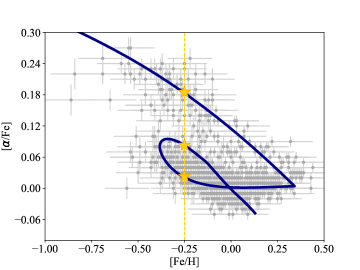
Figure 1: Observed [$\alpha$/Fe] versus [Fe/H] abundance ratios of the APOKASC sample (grey points) presented by Silva Aguirre et al. (2018), compared with the two-infall chemical evolution model characterized by $\tau_{1}=0.1$ Gyr, $\tau_{2}=8$ Gyr, $\sigma_{2}=64$ M_⊙ pc^-2, $\sigma_{2}/\sigma_{1}$=4, $\nu=1.3$ Gyr^-1. The three yellow points clearly show that the predicted chemical evolution curve is multi-valued in this plane (they exhibit three different [$\alpha$/Fe] values for the same [Fe/H] abundance ratio).

To define the likelihood in eq. (5) we assume that the uncertainties on the observables are normally distributed. In that case, the logarithm of the likelihood can be written as,

$$\ln\mathscr{L}=-\sum_{n=1}^{N}\ln\left(\left(2\pi\right)^{d/2}\prod_{j=1}^{d}\sigma_{n,j}\right)-\frac{1}{2}\sum_{n=1}^{N}\sum_{j=1}^{d}\left(\frac{x_{n,j}-\mu_{n,j}}{\sigma_{n,j}}\right)^{2},$$ (6)

where $N$ is the number of stars in the sample and $d$ is the number of observables available. The quantities $x_{n,j}$ and $\sigma_{n,j}$ are respectively the measured value of $j^{\rm th}$ observable and its uncertainty for $n^{\rm th}$ star. In principle, the quantity $\mu_{n,j}$ is the model value of $j^{\rm th}$ observable for $n^{\rm th}$ star, in practice however it is tricky to define (as explained below).

To define $\mu_{n,j}$, we first consider the case of fitting the data only in the [Fe/H]-$[\alpha/{\rm Fe}]$ plane. As can be seen in Fig. 1, the curve predicted by the two-infall model in this plane is multivalued, i.e. there are more than one values of $[\alpha/{\rm Fe}]$ for certain values of [Fe/H]. As a result, it becomes ambiguous to associate an observed data point in the [Fe/H]-$[\alpha/{\rm Fe}]$ plane to a point on the curve, making it difficult to define $\mu_{n,j}$. In this study, we associate a data point to the closest point on the curve. Given a data point $x_{n,j}$, this is done by defining the following function,

$$S_{n}\equiv\min_{i}\left\{\sqrt{\sum_{j=1}^{2}\left(\frac{x_{n,j}-\mu_{n,j,i}}{\sigma_{n,j}}\right)^{2}}\right\}=\sqrt{\sum_{j=1}^{2}\left(\frac{x_{n,j}-\mu_{n,j,i^{\prime}}}{\sigma_{n,j}}\right)^{2}},$$ (7)

where $i$ runs over the different points on the curve. Hence, the closest point on the curve is $\mu_{n,j}=\mu_{n,j,i^{\prime}}$. This definition can be easily generalized to define $\mu_{n,j}$ for an arbitrary number of observables by modifying Eq. 7,

$$S_{n}\equiv\min_{i}\left\{\sqrt{\sum_{j=1}^{d}\left(\frac{x_{n,j}-\mu_{n,j,i}}{\sigma_{n,j}}\right)^{2}}\right\}=\sqrt{\sum_{j=1}^{d}\left(\frac{x_{n,j}-\mu_{n,j,i^{\prime}}}{\sigma_{n,j}}\right)^{2}}.$$ (8)

The computation of the posterior also requires the specification of priors on the model parameters (see eq. 5). Here, we discuss the priors on ${\bf\Theta}=\{\tau_{1},\ \tau_{2},\ t_{\rm max},\ \sigma_{2}/\sigma_{1}\}$ and justify their choices in the current study.

• First infall time-scale $\tau_{1}$: in the classical two-infall model (Chiappini et al., 1997) the first gas infall is characterized by a short time-scale of accretion and it has been fixed at the value of $\tau_{1}$= 1 Gyr. More recently, in order to reproduce the AMBRE thick disc, Grisoni et al. (2017) suggested a smaller value: $\tau_{1}=0.1$ Gyr. In the current study, we set a uniform prior on $\tau_{1}$, exploring the range $0<\tau_{1}<7\mbox{ Gyr}$.

• The second infall time-scale, $\tau_{2}$, is connected to a slower accretion episode. We set a uniform prior on $\tau_{2}$ exploring the range $0<\tau_{2}<28\mbox{ Gyr}$, since there is no reason for $\tau_{2}$ being limited to the age of the Universe.

• The delay $t_{\rm max}$: we set a uniform prior exploring the range $0<t_{\rm max}<14\mbox{ Gyr}$, which extends all the way to the age of the Universe.

• Present-day two surface mass density ratio, $\sigma_{2}/\sigma_{1}$: there are still large discrepancies in the estimates of the thick disc surface density quoted in the literature, which contribute to large uncertainties in the estimates of $\sigma_{2}/\sigma_{1}$. For instance, Nesti & Salucci (2013, and references therein) claimed that the ratio between low- and high-$\alpha$ sequence stars should be around 10. On the other hand, Fuhrmann et al. (2017) derived a local mass density ratio between thin and thick disc stars of 5.26, which becomes as low as 1.73 after correction for the difference in the scale height. While studying APOGEE stars Mackereth et al. (2017) found that the relative contribution of low- to high-$\alpha$ is 5.5. Bearing in mind these uncertainties, we set a uniform prior on the mass density ratio, exploring the range $1<\sigma_{2}/\sigma_{1}<50$ (assuming that the low-$\alpha$ component is more massive than the high-$\alpha$ one).

Finally, we sampled the posterior probability distribution defined by eq. (5) using an affine invariant MCMC ensemble sampler (Goodman & Weare, 2010; Foreman-Mackey et al., 2013). This was accomplished using the publicly available code ”emcee: the mcmc hammer” . We initialized the chains with 100 walkers and ran the sampler for 1000 steps (see below for the details).

4.1 Testing the method

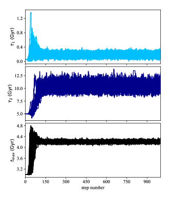
Figure 2: Convergence of the three free model parameters composed by the set ${\bf\Theta}=\{\tau_{1},\ \tau_{2},\ t_{\rm max}\}$ (see model details in Section 4.1) as a function of number of steps.

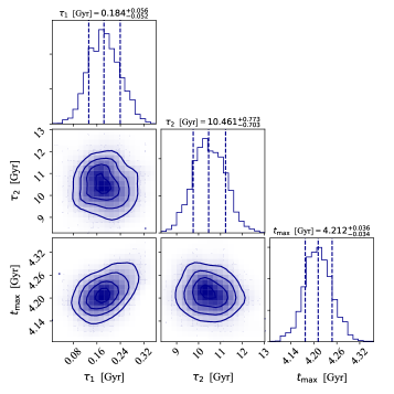
Figure 3: Corner plot showing the posterior PDFs for the same model set as in Fig. 2 obtained by fitting [$\alpha$/Fe] and [Fe/H] abundances from the Silva Aguirre et al. (2018) sample. For each parameter, the median, 16^th and 84^th percentiles of the posterior PDF are plotted above the marginalised PDF.

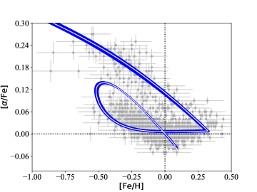
Figure 4: Observed [$\alpha$/Fe] versus [Fe/H] abundance ratios presented by Silva Aguirre et al. (2018) (grey points), compared with model results constrained only by abundance ratio data with three free parameters, composed by the set ${\bf\Theta}=\{\tau_{1},\ \tau_{2},\ t_{\rm max}\}$ (see in Section 4.1). The blue lines correspond to one hundred walkers at the last step, and the thin white line indicates the best fit model.

In this Section we test the method showing results when model free parameters are constrained just by chemical abundance ratios, i.e. the likelihood calculation is based only on [$\alpha$/Fe] and [Fe/H] abundance ratio data. We recall that in ES19, the presence of a significant delay between the two infall episodes ($\sim$ 4.3 Gyr) was a crucial assumption to properly reproduce the APOKASC data.

We consider three free model parameters: the infall time-scales of accretion $\tau_{1}$ (first gas infall), $\tau_{2}$ (second infall), and the delay $t_{{\rm max}}$ between the start of the two infall episodes. The SFE has been fixed to the value of $\nu=1.3$ Gyr^-1, whereas the present-day surface gas density of the high- and low-$\alpha$ sequences are 8 M$\odot$ pc^-2 and 64 M$\odot$ pc^-2, respectively as suggested by the ES19 best model adopting Nesti & Salucci (2013) prescriptions.

It should be noted that the number of steps considered in a MCMC calculation can have a significant impact on the results (Goodman & Weare, 2010; Foreman-Mackey et al., 2013). In Fig. 2 we show the evolution of 100 walkers as a function of the number of steps. As it can be seen, the chains have converged already after 200 steps, thus ensuring the robustness of the results. The posterior probability density function (PDF) of the model parameters is presented in Fig. 3. The best fit model parameters are: $\tau_{1}=0.184^{+0.056}_{-0.052}$ Gyr, $\tau_{2}=10.461^{+0.773}_{-0.703}$ Gyr and $t_{{\rm max}}=4.212^{+0.036}_{-0.034}$ Gyr. In Fig. 4 we show the abundance ratios [$\alpha$/Fe] versus [Fe/H] predicted by 100 walkers computed at the last time-step of the MCMC steps (at the 1000^th step). In this plot the thickness of the model curve represents the uncertainty.

In Fig. 4 we notice that the best model is similar to the one of ES19 (see their Fig. 2), and the associated ”loop” feature in the [$\alpha$/Fe] and [Fe/H] space related to the low-$\alpha$ sequence is retained. The newly constrained free parameter values by the MCMC algorithm are similar to the ones of ES19, and we obtain an almost identical value for the delay $t_{{\rm max}}$ with a difference of $\Delta t_{{\rm max}}=0.088$ Gyr.

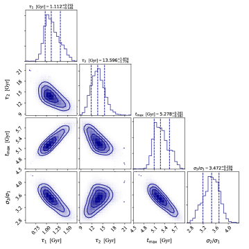
Figure 5: Corner plot showing the posterior PDFs of model M1 in which the SFE has been fixed at the value of $\nu=1.3$ Gyr^-1. In this case the best fit of the four dimensional parameter space ${\bf\Theta}=\{\tau_{1},\ \tau_{2},\ t_{\rm max},\ \sigma_{2}/\sigma_{1}\}$ is obtained by fitting [$\alpha$/Fe], [Fe/H] and ages of the APOKASC sample (see model details in Section 5). The median, 16^th and 84^th percentiles of the posterior PDF are plotted for each parameter above the marginalised PDF.

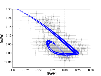
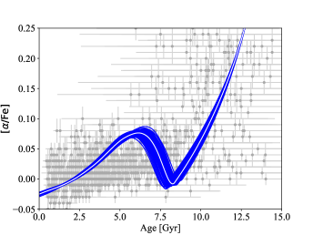
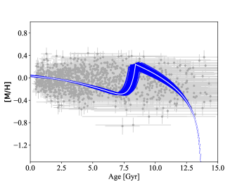
Figure 6: Upper panel: Same as Fig. 4 except that the model M1 is also constrained by means of the APOKASC stellar ages. The best fit model parameters of the set ${\bf\Theta}=\{\tau_{1},\ \tau_{2},\ t_{\rm max},\ \sigma_{2}/\sigma_{1}\}$ was computed by means of the PDFs of Fig. 5. In the Middle and Lower panel the temporal evolution of [$\alpha$/Fe] and the age-metallicity relation are reported, respectively, for the same models and data of the upper panel.

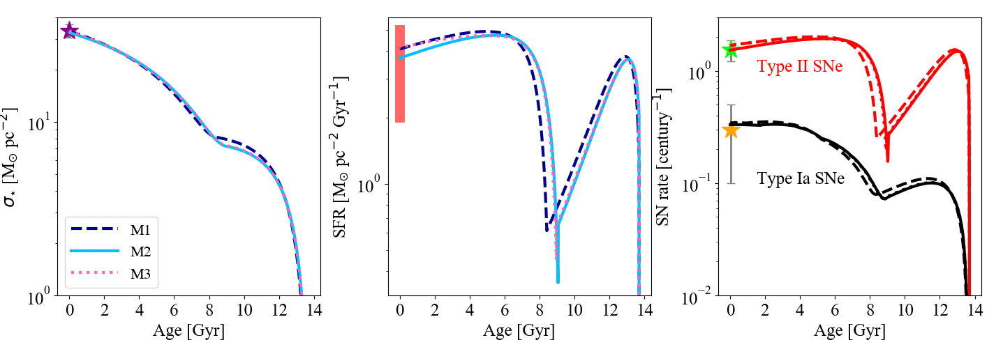
Figure 7: Left panel: Stellar surface mass density $\sigma_{\star}$ evolution predicted by the best fit models M1 (long dashed line), M2 (solid line) and M3 (dotted line). The purple star indicates the observed present-day value given by McKee et al. (2015). Middle panel: same as the left panel for SFR time evolution. The red shaded area indicates the measured range in the solar annulus suggested by Prantzos et al. (2018). Right panel: evolution of the Type Ia SN (black lines) and Type II SN (red lines) rates predicted by models M1, M2 and M3 for the whole Galactic disc. The yellow star stands for the observed Type Ia SN rate observed by Cappellaro & Turatto (1997), whereas the green one stands for Type II SN rates observed by Li et al. (2011).

Table 1: Observed solar chemical abundances compared with the theoretical ones predicted by the best models M1, M2 and M3 (see text for model details) constrained by chemical abundance ratios and stellar ages of the APOKASC sample.

Abundance	Observations	Models
$\log$($X$/H)+12	Asplund et al. (2005)	M1	M2	M3
	[dex]	[dex]	[dex]	[dex]
Fe	7.45$\pm$0.05	7.31	7.31	7.33
Si	7.51$\pm$0.04	7.41	7.40	7.42
Mg	7.53$\pm$0.09	7.44	7.43	7.45

5 Results

In this Section we show model predictions in presence of the new dimension provided by asteroseismology, i.e. precise stellar ages. The free parameters are determined by fitting [$\alpha$/Fe], [Fe/H] and stellar ages provided by the APOKASC sample. We note that, in this analysis, we do not assume the disc component dissection between high-$\alpha$ and low-$\alpha$ stellar sequences by Silva Aguirre et al. (2018) based on the chemistry.

It should be noted that the total surface mass density is another important local key observable. McKee et al. (2015) suggested that the total surface density including the thin and thick components in the solar neighborhood should be 47.1 $\pm$ 3.4 M${}_{\odot}\mbox{ pc}^{-2}$ and that the total local surface density of stars is 33.4 $\pm$ 3 M${}_{\odot}\mbox{ pc}^{-2}$. In this study, we use the value of total surface density (sum of high-$\alpha$ and low-$\alpha$) of 47.1 $\pm$ 3.4 M${}_{\odot}\mbox{ pc}^{-2}$ as provided by McKee et al. (2015) because they also quote constraint on the stellar mass content.

In contrast to Spitoni et al. (2019b), we do not impose the present-day total low-$\alpha$ sequence surface density (see eq. 3) but instead use the total surface mass densities ($\sigma_{tot}=\sigma_{1}+\sigma_{2}$) to be constant as given by the McKee et al. (2015) study. Recalling that $\sigma_{2}/\sigma_{1}$ is the ratio between the low-$\alpha$ and high-$\alpha$ present-day total surface mass density, we have,

$$\sigma_{tot}=\sigma_{2}\left(1+\frac{1}{\sigma_{2}/\sigma_{1}}\right).$$ (9)

Therefore, the values of the present-day surface densities $\sigma_{2}$ and $\sigma_{1}$ to insert in eqs. (3) and (2), respectively are the following ones,

$$\sigma_{2}=\frac{\sigma_{tot}}{\left(1+\frac{1}{\sigma_{2}/\sigma_{1}}\right)}\mbox{ and }\,\sigma_{1}=\sigma_{tot}-\sigma_{2}.$$ (10)

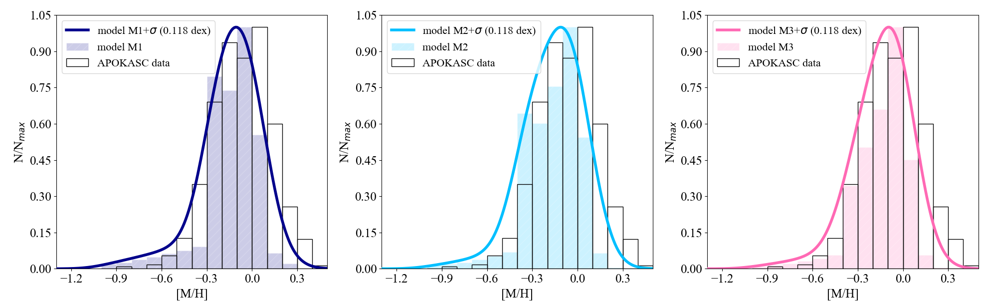
Figure 8: Metallicity distributions predicted by models M1 (left panel), M2 (middle panel) and M3 (right panel) with the best fit model parameters (colored histograms). The observed APOKASC distribution calculated including both high-$\alpha$ and low-$\alpha$ stars is shown by the black, empty histograms. The solid lines indicate the metallicity distribution of our chemical evolution models convolved with a Gaussian with standard deviation $\sigma$ = 0.118 dex (average APOKASC data error). In each plot the distributions are normalised to the corresponding maximum number of stars $N_{max}$.

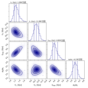
Figure 9: Corner plot showing the posterior PDFs of model M2 in which we adopt different SFEs for the high-$\alpha$ and low-$\alpha$ sequences: $\nu_{1}=2$ Gyr^-1 and $\nu_{2}=1$ Gyr^-1. The best fit of the four dimensional parameter space ${\bf\Theta}=\{\tau_{1},\ \tau_{2},\ t_{\rm max},\ \sigma_{2}/\sigma_{1}\}$ is obtained by fitting [$\alpha$/Fe], [Fe/H] and ages of the APOKASC sample (see model details in Section 5.1). The median, 16^th and 84^th percentiles of the posterior PDF are plotted for each parameter above the marginalised PDF.

We consider, as the reference case, the model with the SFE fixed at the value of $\nu=1.3$ Gyr (model M1) as assumed in ES19 where the predicted solar values for Mg, Fe, and Si were in agreement within one sigma with Asplund et al. (2005) values (see their Table 1). In Fig. 5 we show the corner plot with the posterior PDFs of the model M1 characterized by the four model parameters ${\bf\Theta}=\{\tau_{1},\ \tau_{2},\ t_{\rm max},\ \sigma_{2}/\sigma_{1}\}$ with priors as introduced in Section 4. We still find a significant delay in the start of the second gas infall, even larger than the the value found in ES19, $t_{{\rm max}}=5.278^{+0.261}_{-0.182}$ Gyr. The best model predicts for the $\sigma_{2}/\sigma_{1}$ ratio a value of 3.472${}^{+0.234}_{-0.278}$. Therefore, our analysis favours the value derived by Fuhrmann et al. (2017), whereas the much larger value suggested by Nesti & Salucci (2013) seems unsuitable to reproduce the APOKASC data. Moreover, in the [$\alpha$/Fe] versus [Fe/H] space, this model presents results definitely in agreement with the finding of ES19. Based on a statistical method, we have full confirmation of a significant delay between the two infall episodes, as shown in Fig. 6.

We can see from Table 1 that model M1 predicts Fe solar abundance within $3\sigma$, Si within $2\sigma$ and Mg within $1\sigma$ of the observational estimates by Asplund et al. (2005). The model presented in ES19 was able to reproduce solar values for the above mentioned elements within $1\sigma$. Now we predict smaller solar values compared to ES19 ones because of the longer best fit time-scales of accretion: i.e. $\tau_{1}=1.112^{+0.215}_{-0.145}$ Gyr (first infall) and $\tau_{2}=13.596^{+1.874}_{-1.776}$ Gyr (second infall). Hence, the chemical enrichment for the model M1 is less efficient and evolves slower in time, leading to smaller solar values compared to ES19.

We also notice that the ”loop” in the low-$\alpha$ sequence does not cover all data. We remind the reader that we are considering a model designed for the solar neighborhood and we do not include stellar migration effects. In principle, stellar migration (Schönrich & Binney, 2009) can help in reproducing the low-$\alpha$ sequence composed by stars with the smallest [Fe/H] values (with stars migrating into the solar neighbourhood from the outer disk), as well as with the largest [Fe/H] values (with stellar migration from inner disc regions).

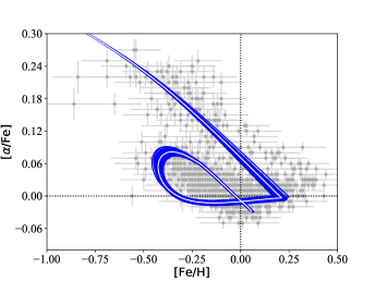
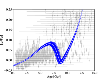
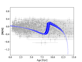
Figure 10: Same as Fig. 6 for model M2 (see in Section 5.1).

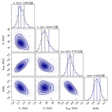
Figure 11: Corner plot showing the posterior PDFs of model M3 in which we adopt different SFEs for the high-$\alpha$ and low-$\alpha$ sequences: $\nu_{1}=2$ Gyr^-1 and $\nu_{2}=1.3$ Gyr^-1 (see model details in Section 5.1). The median, 16^th and 84^th percentiles of the posterior PDF are plotted for each parameter above the marginalised PDF.

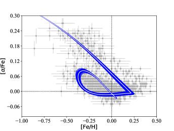
Figure 12: Same as Fig. 6 for model M3 with SFEs fixed at the values of $\nu_{1}=2$ Gyr^.1 $\nu_{2}=1.3$ Gyr^.1 (see model details in Section 5.1).

In Fig. 6, the temporal evolution of the [$\alpha$/Fe] shows an evident ”bump” and the age-metallicity [M/H] relation shows a sudden ”drop”, both signatures of the delayed infall of gas in agreement with ES19 predictions. The presence of such features is not obvious in the observations but could be hidden behind the observational uncertainties. Here we have tested that Bayesian methods lead to best models characterized by significant delay and important gas dilution.

We note that [$\alpha$/Fe] values for the youngest stars tends to fall above the predicted [$\alpha$/Fe] vs. age trend. The predicted slope of the [$\alpha$/Fe] vs age relation for the low-$\alpha$ disc is similar to the one presented by Chiappini et al. (2015) and agrees in fact better with the trend found by Nissen (2016) for solar twin stars in the solar neighborhood than with the APOKASC data.

An important constraint for the chemical evolution model is the present-time stellar surface mass density. The left panel of Fig. 7 shows that our best model predicts a value of 33.28 M${}_{\odot}\mbox{ pc}^{-2}$, in excellent agreement with the value of 33.4 $\pm$ 3 M${}_{\odot}\mbox{ pc}^{-2}$ proposed by McKee et al. (2015). From middle panel of Fig. 7 we notice that the predicted present-day SFR value of 4.08 M_⊙ pc^-2 Gyr^-1 is in agreement with the measured range in the solar vicinity of 2-5 M_⊙ pc^-2 Gyr^-1 (Matteucci, 2012; Prantzos et al., 2018).

Table 2: Predicted delay $t_{{\rm max}}$, present-day surface density ratio $\sigma_{2}$/ $\sigma_{1}$, and infall time-scale $\tau_{1}$ values by the models M1, M2 and M3 presented in this work (see text for model details). In the last column, we also provide the range values admitted by our study. The assumed values for high-$\alpha$ ($\nu_{1}$) and low-$\alpha$ ($\nu_{2}$) SFEs for the different models are also indicated.

		Models
	M1	M2	M3
$\nu_{1}$ [Gyr-1]	1.3	2.0	2.0
$\nu_{2}$ [Gyr-1]	1.3	1.0	1.3
		MCMC Results		Range
$t_{{\rm max}}$ [Gyr]	5.278${}^{+0.261}_{-0.182}$	4.624${}^{+0.135}_{-0.099}$	4.721${}^{+0.126}_{-0.109}$	$4.525-5.539$
$\sigma_{2}$/ $\sigma_{1}$	3.472${}^{+0.234}_{-0.278}$	4.176${}^{+0.167}_{-0.178}$	4.106${}^{+0.166}_{-0.165}$	$3.194-4.334$
$\tau_{1}$ [Gyr]	1.112${}^{+0.215}_{-0.145}$	1.264${}^{+0.119}_{-0.090}$	1.295${}^{+0.119}_{-0.095}$	$0.967-1.414$
$\tau_{2}$ [Gyr]	13.596${}^{+1.874}_{-1.776}$	11.282${}^{+0.954}_{-0.943}$	18.811${}^{+2.598}_{-2.062}$	$10.339-21.409$

The time evolution of the Type Ia SN and Type II SN rates are also plotted in Fig. 7. The present-day Type II SN rate in the whole Galactic disc predicted by our model is 1.67 /[100 yr], in good agreement with the observations of Li et al. (2011) which yield a value of 1.54 $\pm$0.32 /[100 yr]. The predicted present-day Type Ia SN rate in the whole Galactic disc is 0.34 /[100 yr], again in good agreement with the value provided by Cappellaro & Turatto (1997) of 0.30$\pm$0.20 /[100 yr].

In the left panel of Fig. 8 we compare the metallicity distribution function (MDF) of the model M1 with the whole APOKASC data sample. Although the predicted MDF is consistent with the data, it underestimates the number of stars at super-solar metallicities. This is due to the longer best fit time-scales of accretion compared to the classical ”two-infall” model. In Fig. 8 we also draw the curve related to the model distribution convolved with a Gaussian with a constant dispersion fixed at the value of $\sigma=0.118$ dex, which is the average [M/H] observational error in APOKASC data (see ES19). In this case we improve the fit and the high metallicity tail of the MDF is better accounted for.

In the next Section we will test how the delay between the two infall episodes is sensitive to the choice of the SFE parameter.

5.1 SFE parameter study (models M2 and M3)

In this Section we consider different SFE values as already used in previous works. Different infall episodes could in principle be characterized by different SFEs as suggested by Grisoni et al. (2017, 2018). In their chemical evolution models, the SFEs of the high-$\alpha$ and low-$\alpha$ sequences have been fixed at the values of $\nu_{1}=2$ Gyr^-1 and $\nu_{2}=1$ Gyr^-1, respectively.

In model M2 we adopt the same prescriptions as Grisoni et al. (2017, 2018) as shown in Table 2, whereas in model M3 we consider $\nu_{1}=2$ Gyr^-1 and $\nu_{2}=1.3$ Gyr^-1 (high-$\alpha$ SFE as Grisoni et al. 2017 and low-$\alpha$ one as ES19).

In Fig. 9 the corner plot of the posterior PDFs of model M2 confirms the trend mentioned above with model M1. The best value for the time delay is $t_{{\rm max}}=4.624^{+0.135}_{-0.099}$ Gyr, and $\sigma_{2}/\sigma_{1}=4.176^{+0.167}_{-0.178}$. This shows that the time-scales of accretion $\tau_{1}$ and $\tau_{2}$ are sensitive to the assumed SFE. During the high-$\alpha$ phase, the best model M2 is characterized by a longer time-scale $\tau_{1}$ than the M1 one. In order to obtain a chemical enrichment history similar to the one of the M1 model, an increase of the SFE must be compensated by a longer time-scale $\tau_{1}$; the same applies to the second infall timescale.

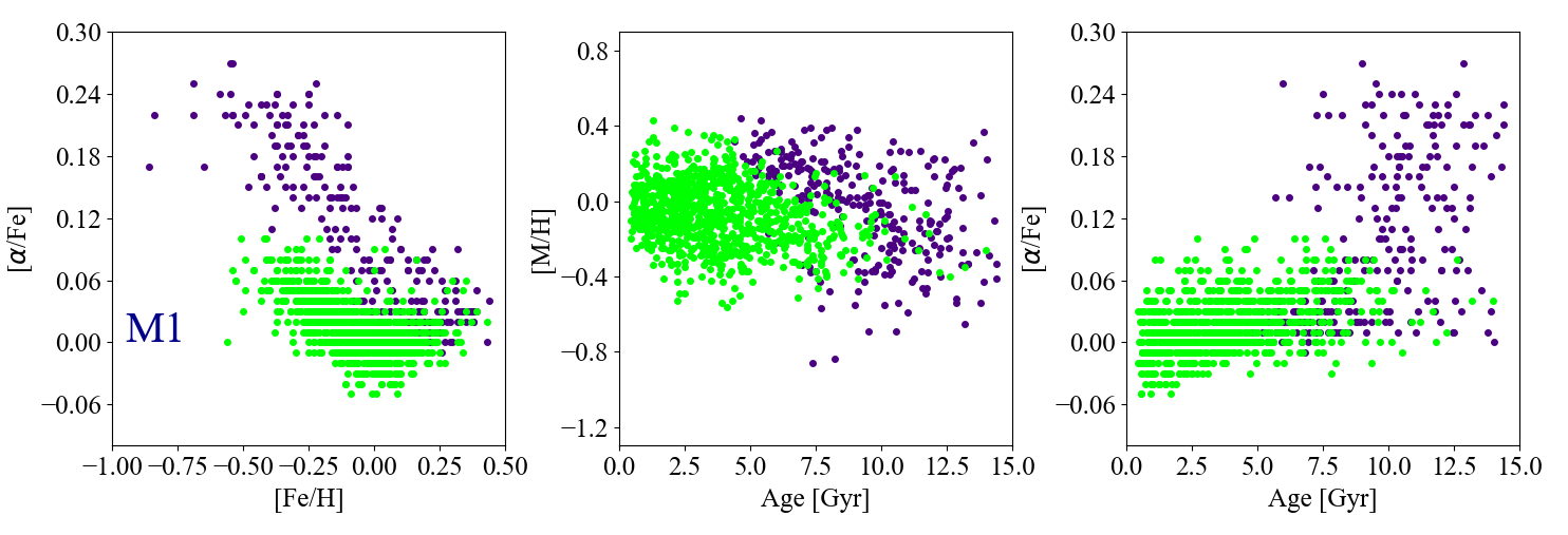
Figure 13: Disc dissection of the APOKASC sample of Silva Aguirre et al. (2018) in high-$\alpha$ (violet points) and low-$\alpha$ (green points) sequence stars based on the chemical evolution model M1. In the left panel the abundance ratios [$\alpha$/Fe] versus [Fe/H] for the APOKASC sample is reported. The age metallicity relation and the temporal evolution of the [$\alpha$/Fe] are shown in the middle and right panels, respectively.

In Fig. 10, it is possible also in this case to appreciate the dilution effect of the gas rich accretion events in the [$\alpha$/Fe] versus [Fe/H] abundance ratios, in the age metallicity relation and in [$\alpha$/Fe] versus age plot. By comparing Fig. 10 with Fig. 6 we note that the two models show similar results.

An important constraint for the chemical evolution model is represented by the present-time stellar surface mass density. The left panel of Fig. 7 shows that our best model M2 predicts a present-time stellar surface mass density value of 32.60 M${}_{\odot}\mbox{ pc}^{-2}$, which is slightly smaller than the value proposed by McKee et al. (2015). The predicted present-day SFR value of 3.72 M_⊙ pc^-2 Gyr^-1 is smaller than the one predicted by M1 model, in better agreement with the observed range of 2-5 M_⊙ pc^-2 Gyr^-1 (Matteucci, 2012; Prantzos et al., 2018).

The present-day Type Ia and II SN rates are also shown in Fig. 7. The present-day Type II SN rate in the whole Galactic disc predicted by our model is 1.53 /[100 yr], in good agreement with the observations by Li et al. (2011). The predicted present-day Type Ia SN rate in the whole Galactic disc is 0.33 /[100 yr], in good agreement with the value provided by Cappellaro & Turatto (1997).

In the middle panel of Fig. 8 we show the MDF for the model M2. We note that the convolution of the MDF with a gaussian of standard deviation equal to the typical [M/H] error in the APOKASC sample helps in reproducing the high- and low-metallicity tails of the observed distribution. Because of the larger SFE value for the high-$\alpha$ sequence $\nu_{1}$, model M2 presents an MDF with more metal poor stars compared to the model M1.

Finally, we present the results related to the model M3 characterized by the following SFEs for the two gas infall episodes: $\nu_{1}=2$ Gyr^-1 and $\nu_{2}=1.3$ Gyr^-1. The corner plot related to the model M3 can be found in Fig. 11. The main difference between model M2 and model M3 is the time-scale of accretion of the second infall $\tau_{2}$; in fact the best fit model M3 requires $\tau_{2}=18.811^{+0.126}_{-0.109}$ Gyr. However, as can be inferred from Figs. 7, 8 and 12 no substantial differences characterize the chemical enrichment of the model M3 compared to models M1 and M2. The model M3 shows a slightly larger solar abundance values (see Tabel 1), because of the higher SFEs in both high-$\alpha$ and low-$\alpha$ sequences.

In Table 2 we summarize the predicted delay $t_{{\rm max}}$, present-day surface density ratio $\sigma_{2}$/$\sigma_{1}$, infall time-scales $\tau_{1}$ and $\tau_{2}$ values obtained for the different best fit models presented in this work. It is clear that in all our tests, independently of the SFE prescription, the presence of a delay is a solid result. In fact, its value spans the range $4.5-5.5$ Gyr. Another important result is that we are capable to constrain the ratio $\sigma_{2}$/$\sigma_{1}$. The predicted values are in the range $3.2-4.3$, in agreement with Fuhrmann et al. (2017) and Mackereth et al. (2017).

The predicted values for $\tau_{1}$, $t_{{\rm max}}$ and $\sigma_{2}$/$\sigma_{1}$ are not much sensitive to different SFE prescriptions, confirming the robustness of the results. However, the best-fit accretion time-scale $\tau_{2}$ spans a large range of values (10.3-21.4 Gyr) considering models M1, M2 and M3. Hence, we cannot draw any firm conclusion about this parameter assuming only the observational constraints given by abundance ratios and ages of the APOKASC sample stars.

The predicted time-scales for the low-$\alpha$ sequence are substantially longer than the one proposed by the classical ”two-infall” model by Chiappini et al. (2001) and Grisoni et al. (2018) for the solar neighborhood. In these works the ”inside-out” formation scenario was obtained with an infall time-scale for the thin disc that increases with the Galactocentric distance, and in particular in the solar neighborhood $\tau_{2}=7$ Gyr (3.3 Gyr smaller than our lower limit predictions). However, the best fit ”low-$\alpha$ ”time-scales of accretions for models M1 and M2 are in agreement with the chemical evolution model proposed by Nidever et al. (2014). In fact, originally designed to reproduce the APOGEE data, this model is characterized by an $e$-folding time-scale of gas accretion fixed at the value of 14 Gyr.

In a future work, it is our intention to extend our results to other Galactocentric distances, analyzing the inside-out Galactic disc growth, with the inclusion of other observational constraints in the MCMC procedure.

5.2 The dissection of the Galactic disc components

In previous works, the Galactic disc dissection in the solar neighbourhood was based either on the chemical tagging or using the kinematics proprieties of the stars (see Silva Aguirre et al. 2018 and references therein). In this Section we propose a new method to separate the APOKASC data in high-$\alpha$ and low-$\alpha$ disc components using the results of our best fit models M1, M2 and M3. We present a new criterium in which, beside the chemical abundance of the stars, we also use their asteroseimic age information.

Given a best fit model, we associate to each star in the space of observables ${\bf x}=\{[\alpha/{\rm Fe}],\ [{\rm Fe}/{\rm H}],\ {\rm age}\}$, the closest point on the model hyper-surface using eq. (8) introduced in Section 4. If this point on the hyper-surface is characterised by an age larger than delay $t_{\rm max}$, then the star is considered as part of the high-$\alpha$ sequence. On the other hand, if this age is smaller than the delay, then it is considered as part of the low-$\alpha$ sequence.

We found that all the models produce roughly the same disc separation, therefore in Fig. 13 we show only the results obtained with the M1 model. It is interesting to note that this dissection criterium produces a disc separation not much different from the one presented by Silva Aguirre et al. (2018) based on chemistry (see their Fig. 8). However, some relevant differences can be noted in the temporal evolution of the abundance ratio [$\alpha$/Fe] for old stars with [$\alpha$/Fe$]<0.05$ dex. The dissection based only on chemistry by Silva Aguirre et al. (2018) tags all the stars in this region as low-$\alpha$ sequence. On the other hand, our separation–which uses the age information as well–predicts a mixed population of high-$\alpha$ and low-$\alpha$ stars close to the delay, $t_{\rm max}$.

By means of a chemo-dynamical model for the Milky Way, it will be possible to include also the kinematic information along with the stellar ages and chemical abundances in the Bayesian analysis based on MCMC methods to better constrain the disc dissection and shed more light to the different disc components.

6 Conclusions

For the first time, we used a detailed Bayesian analysis to constrain chemical evolution models with stellar abundances and precise stellar ages provided by asteroseismology of the APOKASC sample by Silva Aguirre et al. (2018). We tested the robustness of the findings of Spitoni et al. (2019b) concerning the importance of a significant delay between the first infall and the start of the second one in the framework of the two-infall chemical evolution model, in order to reproduce the APOKASC sample in the solar annulus.

In our analysis we considered four free parameters (accretion time-scales $\tau_{1}$ and $\tau_{2}$, delay $t_{\rm max}$ and present-day surface mass density ratio $\sigma_{2}/\sigma_{1}$). We tested three different SFE recipies: in model M1, SFE is fixed at the value of 1.3 Gyr^-1 during the Galactic life, following Grisoni et al. (2017) in model M2 and M3 the high-$\alpha$ and low-$\alpha$ sequences are characterized by different SFEs.

Our main conclusions can be summarized as follows:

• The best fit models M1, M2 and M3 present a delay between the two infall episodes in agreement with Spitoni et al. (2019b). These models also reproduce reasonably well other important observational constraints for the chemical evolution of the disk, including the present-day stellar surface density by McKee et al. (2015), Type II and Type Ia SN rates, the SFR, the metallicity distribution function of the APOKASC data and the solar abundance values of Asplund et al. (2005).

• We have shown with a Bayesian analysis that the presence of a consistent delay is robust against the uncertainties in the SFEs, and the value lies in the range $4.5-5.5$ Gyr for different models.

• The best fit model parameter for present-day surface mass density ratio $\sigma_{2}/\sigma_{1}$ between low-$\alpha$ and high-$\alpha$ sequences spans the range $3.2-4.3$, which is in agreement with the findings of Fuhrmann et al. (2017).

• We used our best models to dissect the Galactic disc components of the APOKASC sample. The results of the dissection are similar to those presented by Silva Aguirre et al. (2018) based only on chemistry. Differences in the disc separations are for the stars close to the model transaction between high-$\alpha$ and low-$\alpha$ sequences in the [$\alpha$/FE] versus [Fe/H] space.

Different physical reasons can be associated to a significant delay in the range $4.5-5.5$ Gyr between the two accretion episodes.

In the two-infall model scenario coupled with the shock-heating theory, a significant delay between the accretion phases has been suggested also by Noguchi (2018) . In their picture, a first infall episode originates the high-$\alpha$ sequence, which is followed by a hiatus until the shock-heated gas in the Galactic dark matter halo has radiatively cooled and can be accreted by the Galaxy. In this framework, Noguchi (2018) found that the SFR of the Galactic disc is characterised by two peaks separated by $\sim 5$ Gyr (in agreement with ES19 and our findings).

The significant delay in the two-infall model of ES19 has been also discussed by Vincenzo et al. (2019) in the context of the stellar system accreted by the Galactic halo, AKA Gaia-Enceladus (Helmi et al., 2018; Koppelman et al., 2019). Vincenzo et al. (2019) presented the first chemical evolution model for Enceladus, investigating the star formation history of one of the most massive satellites accreted by the Milky Way during a major merger event. It was proposed that the mechanism which quenched the Milky Way star formation at high redshift by heating up the gas in the dark matter halo was a major merger event with a satellite like Enceladus. This proposed scenario is in agreement with the recent Chaplin et al. (2020) study. They constrained the merging time with the very bright, naked-eye star $\nu$ Indi finding that, at 68% confidence, the earliest the merger could have started was 11.6 Gyr ago.

Finally, the delay could be interpreted as the main effect of a late gas-rich accretion episode which shaped the low-$\alpha$ sequence, as confirmed in early works of chemical evolution in a cosmological context (Calura & Menci, 2009) and more recently by cosmological simulations (Buck, 2020).

We are aware that our study is limited to the solar annulus region, and that other dynamical processes such as stellar migration (Schönrich & Binney, 2009) might have played an important role during the Galactic evolution.

References

- Asplund et al. (2005) Asplund, M., Grevesse, N., & Sauval, A. J. 2005, in Astronomical Society of the Pacific Conference Series, Vol. 336, Cosmic Abundances as Records of Stellar Evolution and Nucleosynthesis, ed. T. G. Barnes, III & F. N. Bash, 25
- Belfiore et al. (2019) Belfiore, F., Vincenzo, F., Maiolino, R., & Matteucci, F. 2019, MNRAS, 487, 456
- Borucki et al. (2009) Borucki, W., Koch, D., Batalha, N., et al. 2009, in IAU Symposium, Vol. 253, Transiting Planets, ed. F. Pont, D. Sasselov, & M. J. Holman, 289–299
- Brooks et al. (2011) Brooks, S., Gelman, A., Jones, G., & Meng, X.-L. 2011, Handbook of Markov Chain Monte Carlo (CRC press)
- Buck (2020) Buck, T. 2020, MNRAS, 491, 5435
- Calura & Menci (2009) Calura, F. & Menci, N. 2009, MNRAS, 400, 1347
- Cappellaro & Turatto (1997) Cappellaro, E. & Turatto, M. 1997, in NATO Advanced Science Institutes (ASI) Series C, Vol. 486, NATO Advanced Science Institutes (ASI) Series C, ed. P. Ruiz-Lapuente, R. Canal, & J. Isern, 77
- Cescutti et al. (2018) Cescutti, G., Hirschi, R., Nishimura, N., et al. 2018, MNRAS, 478, 4101
- Cescutti et al. (2007) Cescutti, G., Matteucci, F., François, P., & Chiappini, C. 2007, A&A, 462, 943
- Chaplin et al. (2020) Chaplin, W. J., Serenelli, A. M., Miglio, A., et al. 2020, arXiv e-prints, arXiv:2001.04653
- Chiappini et al. (2015) Chiappini, C., Anders, F., Rodrigues, T. S., et al. 2015, A&A, 576, L12
- Chiappini et al. (1997) Chiappini, C., Matteucci, F., & Gratton, R. 1997, ApJ, 477, 765
- Chiappini et al. (2001) Chiappini, C., Matteucci, F., & Romano, D. 2001, ApJ, 554, 1044
- Côté et al. (2017) Côté, B., O’Shea, B. W., Ritter, C., Herwig, F., & Venn, K. A. 2017, ApJ, 835, 128
- Dunkley et al. (2005) Dunkley, J., Bucher, M., Ferreira, P. G., Moodley, K., & Skordis, C. 2005, MNRAS, 356, 925
- Foreman-Mackey et al. (2013) Foreman-Mackey, D., Hogg, D. W., Lang, D., & Goodman, J. 2013, PASP, 125, 306
- François et al. (2004) François, P., Matteucci, F., Cayrel, R., et al. 2004, A&A, 421, 613
- Frankel et al. (2018) Frankel, N., Rix, H.-W., Ting, Y.-S., Ness, M., & Hogg, D. W. 2018, ApJ, 865, 96
- Fuhrmann et al. (2017) Fuhrmann, K., Chini, R., Kaderhandt, L., & Chen, Z. 2017, MNRAS, 464, 2610
- Gaia Collaboration et al. (2016) Gaia Collaboration, Brown, A. G. A., Vallenari, A., et al. 2016, A&A, 595, A2
- Gaia Collaboration et al. (2018) Gaia Collaboration, Katz, D., Antoja, T., et al. 2018, A&A, 616, A11
- García Pérez et al. (2016) García Pérez, A. E., Allende Prieto, C., Holtzman, J. A., et al. 2016, AJ, 151, 144
- Gelman et al. (2013) Gelman, A., Carlin, J., Stern, H., et al. 2013, Bayesian Data Analysis, Third Edition, Chapman & Hall/CRC Texts in Statistical Science (Taylor & Francis)
- Goodman & Weare (2010) Goodman, J. & Weare, J. 2010, Communications in Applied Mathematics and Computational Science, 5, 65
- Grand et al. (2018) Grand, R. J. J., Bustamante, S., Gómez, F. A., et al. 2018, MNRAS, 474, 3629
- Grisoni et al. (2018) Grisoni, V., Spitoni, E., & Matteucci, F. 2018, MNRAS, 481, 2570
- Grisoni et al. (2017) Grisoni, V., Spitoni, E., Matteucci, F., et al. 2017, MNRAS, 472, 3637
- Hayden et al. (2015) Hayden, M. R., Bovy, J., Holtzman, J. A., et al. 2015, ApJ, 808, 132
- Helmi et al. (2018) Helmi, A., Babusiaux, C., Koppelman, H. H., et al. 2018, Nature, 563, 85
- Henriques et al. (2009) Henriques, B. M. B., Thomas, P. A., Oliver, S., & Roseboom, I. 2009, MNRAS, 396, 535
- Henriques et al. (2013) Henriques, B. M. B., White, S. D. M., Thomas, P. A., et al. 2013, MNRAS, 431, 3373
- Hogg & Foreman-Mackey (2018) Hogg, D. W. & Foreman-Mackey, D. 2018, ApJS, 236, 11
- Jaynes (2003) Jaynes, E. T. 2003, Probability Theory: The Logic of Science (Cambridge University Press: Cambridge)
- Jofré et al. (2016) Jofré, P., Jorissen, A., Van Eck, S., et al. 2016, A&A, 595, A60
- Kampakoglou et al. (2008) Kampakoglou, M., Trotta, R., & Silk, J. 2008, MNRAS, 384, 1414
- Kennicutt (1998) Kennicutt, Jr., R. C. 1998, ApJ, 498, 541
- Koppelman et al. (2019) Koppelman, H. H., Helmi, A., Massari, D., Price-Whelan, A. M., & Starkenburg, T. K. 2019, arXiv e-prints, arXiv:1909.08924
- Li et al. (2011) Li, W., Chornock, R., Leaman, J., et al. 2011, MNRAS, 412, 1473
- Lindegren et al. (2016) Lindegren, L., Lammers, U., Bastian, U., et al. 2016, A&A, 595, A4
- Mackereth et al. (2017) Mackereth, J. T., Bovy, J., Schiavon, R. P., et al. 2017, MNRAS, 471, 3057
- Majewski et al. (2017) Majewski, S. R., Schiavon, R. P., Frinchaboy, P. M., et al. 2017, The Astronomical Journal, 154, 0
- Martig et al. (2015) Martig, M., Rix, H.-W., Silva Aguirre, V., et al. 2015, MNRAS, 451, 2230
- Matteucci (2012) Matteucci, F. 2012, Chemical Evolution of Galaxies
- McKee et al. (2015) McKee, C. F., Parravano, A., & Hollenbach, D. J. 2015, ApJ, 814, 13
- Mikolaitis et al. (2017) Mikolaitis, S., de Laverny, P., Recio-Blanco, A., et al. 2017, Astronomy and Astrophysics, 600, A22
- Mott et al. (2013) Mott, A., Spitoni, E., & Matteucci, F. 2013, MNRAS, 435, 2918
- Nesti & Salucci (2013) Nesti, F. & Salucci, P. 2013, J. Cosmology Astropart. Phys., 7, 016
- Nidever et al. (2014) Nidever, D. L., Bovy, J., Bird, J. C., et al. 2014, The Astrophysical Journal, 796, 38
- Nissen (2016) Nissen, P. E. 2016, A&A, 593, A65
- Noguchi (2018) Noguchi, M. 2018, Nature, 559, 585
- Philcox et al. (2018) Philcox, O., Rybizki, J., & Gutcke, T. A. 2018, ApJ, 861, 40
- Pinsonneault et al. (2014) Pinsonneault, M. H., Elsworth, Y., Epstein, C., et al. 2014, ApJS, 215, 19
- Prantzos et al. (2018) Prantzos, N., Abia, C., Limongi, M., Chieffi, A., & Cristallo, S. 2018, MNRAS, 476, 3432
- Putze et al. (2010) Putze, A., Derome, L., & Maurin, D. 2010, A&A, 516, A66
- Recio-Blanco et al. (2014) Recio-Blanco, A., de Laverny, P., Kordopatis, G., et al. 2014, Astronomy and Astrophysics, 567, A5
- Reynolds et al. (2012) Reynolds, C. S., Brenneman, L. W., Lohfink, A. M., et al. 2012, ApJ, 755, 88
- Rojas-Arriagada et al. (2017) Rojas-Arriagada, A., Recio-Blanco, A., de Laverny, P., et al. 2017, Astronomy and Astrophysics, 601, A140
- Rojas-Arriagada et al. (2016) Rojas-Arriagada, A., Recio-Blanco, A., de Laverny, P., et al. 2016, Astronomy and Astrophysics, 586, A39
- Rybizki et al. (2017) Rybizki, J., Just, A., & Rix, H.-W. 2017, A&A, 605, A59
- Salaris et al. (2018) Salaris, M., Cassisi, S., Schiavon, R. P., & Pietrinferni, A. 2018, A&A, 612, A68
- Salaris et al. (1993) Salaris, M., Chieffi, A., & Straniero, O. 1993, ApJ, 414, 580
- Scalo (1986) Scalo, J. M. 1986, Fund. Cosmic Phys., 11, 1
- Schönrich & Binney (2009) Schönrich, R. & Binney, J. 2009, MNRAS, 396, 203
- Sharma (2017) Sharma, S. 2017, ARA&A, 55, 213
- Silva Aguirre et al. (2018) Silva Aguirre, V., Bojsen-Hansen, M., Slumstrup, D., et al. 2018, Monthly Notices of the Royal Astronomical Society, 475, 5487
- Silva Aguirre et al. (2015) Silva Aguirre, V., Davies, G. R., Basu, S., et al. 2015, MNRAS, 452, 2127
- Silva Aguirre et al. (2017) Silva Aguirre, V., Lund, M. N., Antia, H. M., et al. 2017, ApJ, 835, 173
- Speagle (2019) Speagle, J. S. 2019, arXiv e-prints, arXiv:1909.12313
- Spitoni et al. (2019a) Spitoni, E., Cescutti, G., Minchev, I., et al. 2019a, A&A, 628, A38
- Spitoni et al. (2017) Spitoni, E., Gioannini, L., & Matteucci, F. 2017, A&A, 605, A38
- Spitoni & Matteucci (2011) Spitoni, E. & Matteucci, F. 2011, A&A, 531, A72
- Spitoni et al. (2015) Spitoni, E., Romano, D., Matteucci, F., & Ciotti, L. 2015, ApJ, 802, 129
- Spitoni et al. (2019b) Spitoni, E., Silva Aguirre, V., Matteucci, F., Calura, F., & Grisoni, V. 2019b, A&A, 623, A60
- Ural et al. (2015) Ural, U., Wilkinson, M. I., Read, J. I., & Walker, M. G. 2015, Nature Communications, 6, 7599
- Vincenzo et al. (2019) Vincenzo, F., Spitoni, E., Calura, F., et al. 2019, MNRAS, L74
- Yong et al. (2016) Yong, D., Casagrande, L., Venn, K. A., et al. 2016, MNRAS, 459, 487
- Zacharias et al. (2013) Zacharias, N., Finch, C. T., Girard, T. M., et al. 2013, AJ, 145, 44