Efficient Approximation of High-dimensional
Functions With Neural Networks

Abstract

In this paper, we develop a framework for showing that neural networks can overcome the curse of dimensionality in different high-dimensional approximation problems. Our approach is based on the notion of a catalog network, which is a generalization of a standard neural network in which the nonlinear activation functions can vary from layer to layer as long as they are chosen from a predefined catalog of functions. As such, catalog networks constitute a rich family of continuous functions. We show that under appropriate conditions on the catalog, catalog networks can efficiently be approximated with rectified linear unit-type networks and provide precise estimates on the number of parameters needed for a given approximation accuracy. As special cases of the general results, we obtain different classes of functions that can be approximated with ReLU networks without the curse of dimensionality.

I Introduction

Many classical numerical approximation schemes that work well in low dimensions suffer from the so called curse of dimensionality, meaning that to achieve a desired approximation accuracy, their complexity has to grow exponentially in the dimension. On the other hand, neural networks have shown remarkable performance in different high-dimensional approximation problems. In this paper we prove that different classes of high-dimensional functions admit a neural network approximation without the curse of dimensionality. To do that, we introduce the notion of a catalog network, which is a generalization of a standard feedforward neural network in which the nonlinear activation functions can vary from one layer to another as long as they are chosen from a given catalog of continuous functions. We first study the approximability of different catalogs with neural networks. Then we show how the approximability of a catalog translates into the approximability of the corresponding catalog networks. An important building block of our proofs is a new way of parallelizing networks that saves parameters compared to the standard parallelization. As special cases of our general results we obtain that different combinations of one-dimensional Lipschitz functions, sums, maxima and products as well as certain ridge functions and generalized Gaussian radial basis function networks admit a neural network approximation without the curse of dimensionality.

It has been shown that neural networks with a single hidden layer can approximate any finite-dimensional continuous function uniformly on compact sets arbitrarily well if they are allowed to have sufficiently many hidden neurons; see, e.g., [Funahashi1989, Cybenko1989, HorStinWhite1989, Hornik1991, LeshnoLinPinkusScho1993, GuliIsm2018b]. Moreover, [Jones1992] and [Barron1993] have proved an $\mathcal{O}(n^{-1/2})$-rate for approximating functions in the $L^{2}$-norm with single-hidden-layer sigmoidal networks with $n$ neurons. In particular, this breaks the curse of dimensionality, but it only applies to a special class of functions. Since then, their results have been applied and generalized in different directions, always yielding rates of the same nature, but always applicable only to similarly restricted classes of functions. For example, in [DonGurvDarSont1997, GirAnz1993] these results have been extended to the $L^{p}$-norm for $1\leq p<\infty$ and $p=\infty$, respectively, and in [KurSang2008] the approximation rate has been improved to a geometric rate for single functions. However, the basis $\delta$ of the geometric rate $\mathcal{O}((1-\delta)^{n})$ is usually not known. So, it could be so small that the geometric rate does not give useful bounds for typical sizes of $n$. For further generalizations, see, e.g., [Barron1992, Barron1994, GurvKoir1997, KlusBar2018, KurKaiKre1997, KurSang2002, Kurkova2008, KaiKurSang2009, KaiKurSang2012]. All of them use single-hidden-layer networks. However, neural networks with more than one hidden layer have shown better performance in a number of applications; see, e.g., [LeCun2015, GoodfBengioCourv2016] and the references therein. This has also been supported by theoretical evidence; for instance, in [EldanShamir2016], an example of a simple continuous function on $\mathbb{R}^{d}$ has been given that is expressible as a small feedforward network with two hidden layers but cannot be approximated with a single-hidden-layer network to a given constant accuracy unless its width is exponential in the dimension. Similarly, it has been shown in [SafranShamir2017] that indicator functions of $d$-dimensional balls can be approximated much more efficiently with two hidden layers than with one. Related results for functions on the product of two $d$-dimensional spheres have been provided by [Daniely2017].

[Pinkus1999, MaioPinkus1999, GuliIsm2018a] have constructed special activation functions which, in principle, allow to approximate every continuous function $f\colon[0,1]^{d}\to\mathbb{R}$ to any desired precision when used in a two-hidden-layers network with as few as $d$ neurons in the first and $2d+2$ neurons in the second hidden layer. Theoretically, this breaks the curse of dimensionality quite spectacularly. However, it can be shown that the approximation result only holds if the size of the network weights is allowed to grow faster than polynomially in the inverse of the approximation error; see, e.g., [BolcGrohsKutynPete2019, PeteVoigt2018].

Further studies of the approximation capacity of neural networks with standard activation functions include, e.g, [Mhaskar1993, VoigtPete2019, PeteVoigt2018, LuShenYangZhang2020, Yarotsky2017]. Their approach is based on approximating functions with polynomials and then approximating these polynomials with neural networks. Polynomials can approximate smooth functions reasonably well, and neural networks are known to be able to approximate monomials efficiently. However, since the number of monomials needed to generate all polynomials in $d$ variables of order $k$ is $\binom{k+d}{d}$, the intermediate step from monomials to polynomials introduces a curse of dimensionality. It has been shown in [Yarotsky2017] that this cannot be side-stepped. For instance, it is provably impossible to approximate the unit ball in the Sobolev space of any regularity with ReLU networks without the curse of dimensionality. So, to overcome the curse of dimensionality with ReLU networks, one has to concentrate on special classes of functions. [Jones1992, Barron1993] and their extensions offer one such class. Coming from a different angle, [MhasMicc1994] has obtained the same rate for periodic functions with an absolutely convergent Fourier series. In [SchwabZech2019] the approximability of “separately holomorphic” maps via Taylor expansions and applications to parametric PDEs have been studied. The approach of [SchwabZech2019] is again based on the intermediate approximation of polynomials, but the holomorphy ensures that the approximating polynomials contain only few monomials. [GrohsHorJenWurs2018, JenSaliWelti2018, HutzJenKruseNguyen2020] have proved that solutions of various PDEs admit neural network approximations without the curse of dimensionality. Their arguments use the hierarchic structure of neural networks, which has more extensively been exploited in [LeeGeMaRistArora2017, BolcGrohsKutynPete2019, GrohsPerekElbBolc2019]. These papers are similar in spirit to ours since they also start from a “basis” of functions, which they approximate with neural networks and then use to build more complex functions. However, [BolcGrohsKutynPete2019, GrohsPerekElbBolc2019] do not study approximation rates in terms of the dimension. On the other hand, in [LeeGeMaRistArora2017] the curse of dimensionality is overcome, but the “basis” in [LeeGeMaRistArora2017] consists of the functions considered in [Barron1993]. In this paper we consider more explicit classes of functions and provide bounds on the number of parameters needed to approximate $d$-dimensional functions up to accuracy $\varepsilon$.

The rest of the paper is organized as follows. In Section II, we first establish the notation. Then we recall basic facts from [PeteVoigt2018, GrohsHorJenZimm2019, JenSaliWelti2018] on concatenating and parallelizing neural networks before we introduce a new way of network parallelization. In Section III, we introduce the concepts of an approximable catalog and a catalog network. Section IV is devoted to different concrete examples of catalogs and a careful study of their approximability. In Sections V and VI, we derive bounds on the number of parameters needed to approximate a given catalog network to a desired accuracy with neural networks. Theorems 19 and 26 are the main results of this article. In Section VII, we derive different classes of high-dimensional functions that are approximable with ReLU networks without the curse of dimensionality. Section VIII concludes. All proofs are relegated to the Appendix.

II Notation and Preliminary Results

A neural network encodes a succession of affine and non-linear transformations. Let us denote $\mathbb{N}=\{1,2,\dots\}$ and consider the set of neural network skeletons

$$\mathcal{N}=\bigcup_{D\in\mathbb{N}}\bigcup_{(l_{0},\dots,l_{D})\in\mathbb{N}^{D+1}}\prod_{k=1}^{D}(\mathbb{R}^{l_{k}\times l_{k-1}}\times\mathbb{R}^{l_{k}}).$$

We denote the depth of a neural network skeleton $\phi\in\mathcal{N}$ by $\mathcal{D}(\phi)=D$, the number of neurons in the $k$th layer by $l_{k}^{\phi}=l_{k}$, $k\in\{0,\dots,D\}$, and the number of network parameters by $\mathcal{P}(\phi)=\sum_{k=1}^{D}l_{k}(l_{k-1}+1)$. Moreover, if $\phi\in\mathcal{N}$ is given by $\phi=[(V_{1},b_{1}),\dots,(V_{D},b_{D})]$, we denote by $\mathcal{A}_{k}^{\phi}\in C(\mathbb{R}^{l_{k-1}},\mathbb{R}^{l_{k}})$, $k\in\{1,\dots,D\}$, the affine function $x\mapsto V_{k}x+b_{k}$. Let $a\colon\mathbb{R}\to\mathbb{R}$ be a continuous activation function. As usual, we extend it, for every positive integer $d$, to a function from $\mathbb{R}^{d}$ to $\mathbb{R}^{d}$ mapping $(x_{1},\dots,x_{d})$ to $(a(x_{1}),\dots,a(x_{d}))$. Then the $a$-realization of $\phi\in\mathcal{N}$ is the function $\mathcal{R}_{a}^{\phi}\in C(\mathbb{R}^{l_{0}},\mathbb{R}^{l_{D}})$ given by

$$\mathcal{R}_{a}^{\phi}=\mathcal{A}_{D}^{\phi}\circ a\circ\mathcal{A}_{D-1}^{\phi}\circ\cdots a\circ\mathcal{A}_{1}^{\phi}.$$

We recall that suitable $\phi_{1},\phi_{2}\in\mathcal{N}$ can be composed such that the $a$-realization of the resulting network equals the concatenation $\mathcal{R}_{a}^{\phi_{2}}\circ\mathcal{R}_{a}^{\phi_{1}}$. This is done by combining the output layer of $\phi_{1}$ with the input layer of $\phi_{2}$. More precisely, if $\phi_{1}=[(V_{1},b_{1}),\dots,(V_{D},b_{D})]$ and $\phi_{2}=[(W_{1},c_{1}),\dots,(W_{E},c_{E})]$ satisfy $l_{\mathcal{D}(\phi_{1})}^{\phi_{1}}=l_{0}^{\phi_{2}}$, then the concatenation $\phi_{2}\circ\phi_{1}\in\mathcal{N}$ is given by

$$\begin{split}\phi_{2}\circ\phi_{1}=[&(V_{1},b_{1}),\dots,(V_{D-1},b_{D-1}),\\ &(W_{1}V_{D},W_{1}b_{D}+c_{1}),(W_{2},c_{2}),\dots,(W_{E},c_{E})].\end{split}$$

The following result is straight-forward from the definition. A formal proof can be found in [GrohsHorJenZimm2019].

Proposition 1.

The concatenation

$$(\cdot)\circ(\cdot)\colon\{(\phi_{1},\phi_{2})\in\mathcal{N}\times\mathcal{N}\colon l_{\mathcal{D}(\phi_{1})}^{\phi_{1}}=l_{0}^{\phi_{2}}\}\rightarrow\mathcal{N}$$

is associative and for all $\phi_{1},\phi_{2}\in\mathcal{N}$ with $l_{\mathcal{D}(\phi_{1})}^{\phi_{1}}=l_{0}^{\phi_{2}}$ one has

1. $\mathcal{R}_{a}^{\phi_{2}\circ\phi_{1}}=\mathcal{R}_{a}^{\phi_{2}}\circ\mathcal{R}_{a}^{\phi_{1}}$ for all $a\in C(\mathbb{R},\mathbb{R})$,

2. $\mathcal{D}(\phi_{2}\circ\phi_{1})=\mathcal{D}(\phi_{1})+\mathcal{D}(\phi_{2})-1$,

3. $l_{k}^{\phi_{2}\circ\phi_{1}}=l_{k}^{\phi_{1}}$ if $k\in\{0,\dots,\mathcal{D}(\phi_{1})-1\}$,

4. $l_{k}^{\phi_{2}\circ\phi_{1}}=l_{k+1-\mathcal{D}(\phi_{1})}^{\phi_{2}}$ if $k\in\{\mathcal{D}(\phi_{1}),\dots,\mathcal{D}(\phi_{2}\circ\phi_{1})\}$,

5. $\mathcal{P}(\phi_{2}\circ\phi_{1})=\mathcal{P}(\phi_{1})+\mathcal{P}(\phi_{2})+l_{1}^{\phi_{2}}l_{\mathcal{D}(\phi_{1})-1}^{\phi_{1}}-l_{0}^{\phi_{2}}l_{1}^{\phi_{2}}-l_{\mathcal{D}(\phi_{1})}^{\phi_{1}}(l_{\mathcal{D}(\phi_{1})-1}^{\phi_{1}}+1)$,

6. $\mathcal{P}(\phi_{2}\circ\phi_{1})\leq\mathcal{P}(\phi_{1})$ if $\mathcal{D}(\phi_{2})=1$ and $l_{1}^{\phi_{2}}\leq l_{\mathcal{D}(\phi_{1})}^{\phi_{1}}$

7. and $\mathcal{P}(\phi_{2}\circ\phi_{1})\leq\mathcal{P}(\phi_{2})$ if $\mathcal{D}(\phi_{1})=1$ and $l_{0}^{\phi_{1}}\leq l_{0}^{\phi_{2}}$.

The next lemma is a direct consequence of the above and will be used later to estimate the number of parameters in our approximating networks.

Lemma 2.

Let $a\in C(\mathbb{R},\mathbb{R})$ and $\phi\in\mathcal{N}$. Suppose that $\psi_{1},\psi_{2}\in\mathcal{N}$ satisfy $\mathcal{D}(\psi_{1})=\mathcal{D}(\psi_{2})=2$, $l_{0}^{\psi_{1}}=l_{2}^{\psi_{1}}=l_{0}^{\phi}$ and $l_{0}^{\psi_{2}}=l_{2}^{\psi_{2}}=l_{\mathcal{D}(\phi)}^{\phi}$. Denote $m=l_{1}^{\psi_{1}}$ if $\mathcal{D}(\phi)=1$ and $m=l_{\mathcal{D}(\phi)-1}^{\phi}$ if $\mathcal{D}(\phi)\geq 2$. Then

$$\begin{split}\mathcal{P}(\psi_{2}\circ\phi\circ\psi_{1})&=\mathcal{P}(\phi)+l_{1}^{\psi_{1}}(l_{0}^{\phi}+1)+l_{1}^{\psi_{2}}(l_{\mathcal{D}(\phi)}^{\phi}+1)\\ &\quad+l_{1}^{\phi}(l_{1}^{\psi_{1}}-l_{0}^{\phi})+m(l_{1}^{\psi_{2}}-l_{\mathcal{D}(\phi)}^{\phi}).\end{split}$$

The standard parallelization of two network skeletons $\phi_{1}=[(V_{1},b_{1}),\dots,(V_{D},b_{D})]$ and $\phi_{2}=[(W_{1},c_{1}),\dots,(W_{D},c_{D})]$ of the same depth is given by $p(\phi_{1},\phi_{2})=$

$$\bigg{[}\bigg{(}\begin{bmatrix}V_{1}&0\\ 0&W_{1}\end{bmatrix},\begin{bmatrix}b_{1}\\ c_{1}\end{bmatrix}\bigg{)},\dots,\bigg{(}\begin{bmatrix}V_{D}&0\\ 0&W_{D}\end{bmatrix},\begin{bmatrix}b_{D}\\ c_{D}\end{bmatrix}\bigg{)}\bigg{]}.$$

From there, arbitrarily many network skeletons $\phi_{1},\dots,\phi_{n}\in\mathcal{N}$, $n\in\mathbb{N}_{\geq 3}$, of the same depth can be parallelized iteratively:

$$p(\phi_{1},\dots,\phi_{n})=p(p(\phi_{1},\dots,\phi_{n-1}),\phi_{n}).$$

The first three statements of the next proposition follow immediately from the definition. The last one is shown in [GrohsHorJenZimm2019].

Proposition 3.

The parallelization

$$p\colon\bigcup_{n\in\mathbb{N}}\{(\phi_{1},\dots,\phi_{n})\in\mathcal{N}^{n}\colon\mathcal{D}(\phi_{1})=\dots=\mathcal{D}(\phi_{n})\}\rightarrow\mathcal{N}$$

satisfies for all $\phi_{1},\dots,\phi_{n}\in\mathcal{N}$, $n\in\mathbb{N}$, with the same depth

1. $\mathcal{R}_{a}^{p(\phi_{1},\dots,\phi_{n})}(x_{1},\dots,x_{n})=(\mathcal{R}_{a}^{\phi_{1}}(x_{1}),\dots,\mathcal{R}_{a}^{\phi_{n}}(x_{n}))$ for all $x_{1}\in\mathbb{R}^{l_{0}^{\phi_{1}}},\dots,x_{n}\in\mathbb{R}^{l_{0}^{\phi_{n}}}$ and each $a\in C(\mathbb{R},\mathbb{R})$,

2. $l_{k}^{p(\phi_{1},\dots,\phi_{n})}=\sum_{j=1}^{n}l_{k}^{\phi_{j}}$ for all $k\in\{0,\dots,\mathcal{D}(\phi_{1})\}$,

3. $\mathcal{P}(p(\phi_{1},\dots,\phi_{n}))\leq n^{2}\mathcal{P}(\phi_{1})$ whenever $l_{k}^{\phi_{i}}=l_{k}^{\phi_{j}}$ for all $k\in\{0,\dots,\mathcal{D}(\phi_{1})\}$ and all $i,j\in\{1,\dots,n\}$

4. and $\mathcal{P}(p(\phi_{1},\dots,\phi_{n}))\leq\frac{1}{2}\big{[}\sum_{j=1}^{n}\mathcal{P}(\phi_{j})\big{]}^{2}$.

Neural networks with different depths can still be parallelized, but only for a special class of activation functions.

Definition 4.

We say a function $a\in C(\mathbb{R},\mathbb{R})$ fulfills the $c$-identity requirement for a number $c\geq 2$ if there exists $I\in\mathcal{N}$ such that $\mathcal{D}(I)=2$, $l_{1}^{I}\leq c$ and $\mathcal{R}_{a}^{I}=\mathrm{id}_{\mathbb{R}}$.

Note that if $I$ satisfies $\mathcal{R}_{a}^{I}=\mathrm{id}_{\mathbb{R}}$, one can also realize the identity function $\mathrm{id}_{\mathbb{R}^{d}}$ for any $d\in\mathbb{N}$, using $d$-fold parallelization $I_{d}=p(I,\dots,I)$. Obviously, $l_{1}^{I_{d}}\leq cd$.

The most prominent example satisfying Definition 4 is the rectified linear unit activation $\mathrm{ReLU}\colon\mathbb{R}\rightarrow\mathbb{R},~{}x\mapsto\max\{x,0\}$. It fulfills the $2$-identity requirement with $I=[([1\ -1]^{T},[0\ 0]^{T}),$ $([1\ -1],0)]$. However, it is easy to see that generalized ReLU functions of the form

$$a(x)=\begin{cases}rx&\mbox{ if }x\geq 0\\ sx&\mbox{ if }x<0\end{cases}$$

for $(r,s)\in\mathbb{R}^{2}$ with $r+s\neq 0$, such as leaky ReLU, also satisfy the $2$-identity requirement.

Figure 1: Parallelization of a network $\phi_{1}$ (depth 4) and a shorter network $\phi_{2}$ (depth 2) obtained by concatenating $\phi_{2}$ twice with a network $I$ arising from the 2-identity requirement, resulting in $\tilde{\phi}_{2}=I\circ I\circ\phi_{2}$.

Using the identity requirement, one can parallelize networks of arbitrary depths. If $\phi_{1},\dots,\phi_{n}\in\mathcal{N}$ have different depths, one simply concatenates the shorter ones with identity networks until all have the same depth. Then one applies the standard parallelization; see Figure 1 for an illustration.

Figure 2: The parallelization of $\phi_{1}$ with architecture $(1,l,1,1)$ and $\phi_{2}$ with architecture $(1,1,l,1)$ has more than $l^{2}$ parameters.

Although this successfully parallelizes networks with arbitrary architecture, one can do better in terms of parameter counts. The estimate in Proposition 3.(4) contains a square of $\sum_{j=1}^{n}\mathcal{P}(\phi_{j})$. This is not due to lax estimates, but a square can actually appear if, for some $j$, there are two large consecutive layers in $p(\phi_{j},\phi_{j+1})$ which in $\phi_{j}$ and $\phi_{j+1}$ were next to small layers; see Figure 2. To avoid this, we introduce a new parallelization which uses identity networks to shift $\phi_{1},\dots,\phi_{n}$ away from each other and, as a result, achieves a parameter count that is linear in $\sum_{j=1}^{n}\mathcal{P}(\phi_{j})$. For instance, to parallelize $\phi_{1}$ and $\phi_{2}$, we add $\mathcal{D}(\phi_{2})$ identity networks after $\phi_{1}$ and $\mathcal{D}(\phi_{1})$ identity networks in front of $\phi_{2}$ before applying $p$. The realization of the resulting network still is $(x_{1},x_{2})\mapsto(\mathcal{R}_{a}^{\phi_{1}}(x_{1}),\mathcal{R}_{a}^{\phi_{2}}(x_{2}))$. Extending this construction to more than two networks is straight-forward; see Figure 3. We denote it by $p_{I}$, where $I\in\mathcal{N}$ is the network satisfying the identity requirement. The following proposition shows that $p_{I}$ achieves our goal of a linear parameter count in $\mathop{\textstyle{\sum}}_{j=1}^{n}\mathcal{P}(\phi_{j})$.

Figure 3: New “diagonalized” parallelization resulting from shifting $\phi_{1},\phi_{2},\phi_{3}$ away from each other.

Proposition 5.

Assume $a\in C(\mathbb{R},\mathbb{R})$ fulfills the $c$-identity requirement for a number $c\geq 2$ with $I\in\mathcal{N}$. Then the parallelization $p_{I}\colon\bigcup_{n\in\mathbb{N}}\mathcal{N}^{n}\rightarrow\mathcal{N}$ satisfies

$$\mathcal{P}(p_{I}(\phi_{1},\dots,\phi_{n}))\leq\big{(}\tfrac{11}{16}c^{2}l^{2}n^{2}-1\big{)}\mathop{\textstyle{\sum}}_{j=1}^{n}\mathcal{P}(\phi_{j})$$

for all $n\in\mathbb{N}$ and $\phi_{1},\dots,\phi_{n}\in\mathcal{N}$, where we denote $l=\max_{j\in\{1,\dots,n\}}\max\{l_{0}^{\phi_{j}},l_{\mathcal{D}(\phi_{j})}^{\phi_{j}}\}$.

It can be seen from the proof that the inequality of Proposition 5 is never an equality. However, it can be shown that it is asymptotically sharp up to a constant for large $n$. Indeed, if $c=2$ (as is the case for $\mathrm{ReLU}$) and if $\phi_{1}=\dots=\phi_{n}$ has depth at least two ($\mathcal{D}(\phi_{1})\geq 2$) and a single neuron in each layer ($l_{k}^{\phi_{1}}=1$ for all $k$), then

$$(2n^{3}-n^{2})\mathcal{P}(\phi_{1})=\mathcal{P}(p_{I}(\phi_{1},\dots,\phi_{n}))\leq\big{(}\tfrac{11}{4}n^{3}-n\big{)}\mathcal{P}(\phi_{1}).$$

The first inequality is verified in the Appendix while the second one is a consequence of Proposition 5. Hence, the bound in the proposition is asymptotically sharp up to a factor of at most $\frac{11}{8}$.

Proposition 5 illustrates that there is a fundamental difference between counting the number of neurons and counting the number of parameters. As already observed in [PeteVoigt2018, GrohsHorJenZimm2019, JenSaliWelti2018], this also plays a role for the concatenation. The standard concatenation of two networks $\phi_{1}$ and $\phi_{2}$ has roughly ${\cal P}(\phi_{1})+{\cal P}(\phi_{2})$ neurons. But the parameter count may increase much more dramatically. If, e.g., most of the neurons of $\phi_{1}$ are in the last hidden layer and most of the neurons of $\phi_{2}$ in the first hidden layer, then $\phi_{2}\circ\phi_{1}$ has roughly $\mathcal{P}(\phi_{1})\cdot\mathcal{P}(\phi_{2})$ parameters; see Figure 4. To counter this, one can use the concatenation

$$I_{l^{\phi_{2}}_{{\cal D}(\phi_{2})}}\circ\phi_{2}\circ I_{l^{\phi_{2}}_{0}}\circ I_{l^{\phi_{1}}_{{\cal D}(\phi_{1})}}\circ\phi_{1}\circ I_{l^{\phi_{1}}_{0}}$$

instead of $\phi_{2}\circ\phi_{1}$, where $I_{d}$ is an identity network in $d$ dimensions. Even though this results in more neurons, it reduces the parameter count. The following estimate is a consequence of Lemma 2.

Corollary 6.

Assume $a\in C(\mathbb{R},\mathbb{R})$ satisfies the $c$-identity requirement for a number $c\geq 2$ with $I\in\mathcal{N}$ and denote $I_{d}=p(I,\dots,I)$ for all $d\in\mathbb{N}$. Let $\phi\in\mathcal{N}$ and abbreviate $m=\max\{l_{0}^{\phi},l_{\mathcal{D}(\phi)}^{\phi}\}$. Then

$$\mathcal{P}(I_{l_{\mathcal{D}(\phi)}^{\phi}}\circ\phi\circ I_{l_{0}^{\phi}})\leq\tfrac{5}{6}cm\mathcal{P}(\phi)+\tfrac{29}{12}c^{2}m^{2}.$$

This will be used in our proofs to estimate the number of parameters of

$$I_{l^{\phi_{2}}_{{\cal D}(\phi_{2})}}\circ\phi_{2}\circ I_{l^{\phi_{2}}_{0}}\circ I_{l^{\phi_{1}}_{{\cal D}(\phi_{1})}}\circ\phi_{1}\circ I_{l^{\phi_{1}}_{0}}.$$

Figure 4: Concatenation with and without additional identity networks. Here, $\phi$ is a network of depth 2 with $l$ neurons in its hidden layer, and $I$ is assumed to satisfy the 2-identity requirement.

III Catalog Networks

In this section, we generalize the concept of a neural network by allowing the activation functions to change from one layer to the next as long as they belong to a predefined catalog $\mathcal{F}\subseteq\bigcup_{m,n\in\mathbb{N}}C(\mathbb{R}^{m},\mathbb{R}^{n})$. We denote the dimension of the domain of a function $f\in\bigcup_{m,n\in\mathbb{N}}C(\mathbb{R}^{m},\mathbb{R}^{n})$ by $\mathcal{I}(f)$ and the dimension of its target space by $\mathcal{O}(f)$, so that $f\in C(\mathbb{R}^{\mathcal{I}(f)},\mathbb{R}^{\mathcal{O}(f)})$. For a catalog $\mathcal{F}$ and numbers $D\in\mathbb{N}$, $l_{0},\dots,l_{2D}\in\mathbb{N}$, we define $\mathcal{C}_{\mathcal{F}}^{l_{0},\dots,l_{2D}}$ as

$$\begin{split}\prod_{k=1}^{D}\bigg{[}\mathbb{R}^{l_{2k-1}\times l_{2k-2}}\times\mathbb{R}^{l_{2k-1}}\times\bigcup_{n\in\mathbb{N}}\Big{\{}(f_{1},\dots,f_{n})\in\mathcal{F}^{n}\colon\\ \sum_{j=1}^{n}\mathcal{I}(f_{j})=l_{2k-1}\text{ and }\sum_{j=1}^{n}\mathcal{O}(f_{j})=l_{2k}\Big{\}}\bigg{]}.\end{split}$$

The set of all catalog networks corresponding to $\mathcal{F}$ is given by

$$\mathcal{C}_{\mathcal{F}}=\bigcup_{D\in\mathbb{N}}\bigcup_{l_{0},\dots,l_{2D}\in\mathbb{N}}\mathcal{C}_{\mathcal{F}}^{l_{0},\dots,l_{2D}}.$$

An element $\xi\in\mathcal{C}_{\mathcal{F}}^{l_{0},\dots,l_{2D}}$ is of the form $\xi=[(V_{1},b_{1},\allowbreak(f_{1,1},\dots,f_{1,n_{1}})),\allowbreak\dots,\allowbreak(V_{D},b_{D},\allowbreak(f_{D,1},\dots,f_{D,n_{D}}))]$. For each $k\in\{1,\dots,D\}$, we let $\mathcal{A}^{\xi,k}\in C(\mathbb{R}^{l_{2k-2}},\mathbb{R}^{l_{2k-1}})$ be the affine function $x\mapsto V_{k}x+b_{k}$. By $\mathcal{G}^{\xi,k}\in C(\mathbb{R}^{l_{2k-1}},\mathbb{R}^{l_{2k}})$, we denote the function mapping $x\in\mathbb{R}^{l_{2k-1}}$ to

$$\begin{split}\mathcal{G}^{\xi,k}(x)=\big{[}&f_{k,1}\big{(}x_{1},\ldots,x_{\mathcal{I}(f_{k,1})}\big{)},\\ &f_{k,2}\big{(}x_{\mathcal{I}(f_{k,1})+1},\ldots,x_{\mathcal{I}(f_{k,1})+\mathcal{I}(f_{k,2})}\big{)},\dots,\\ &f_{k,n_{k}}\big{(}x_{\mathcal{I}(f_{k,1})+\cdots+\mathcal{I}(f_{k,n_{k}-1})+1},\dots,\\ &\qquad\qquad\qquad\qquad x_{\mathcal{I}(f_{k,1})+\cdots+\mathcal{I}(f_{k,n_{k}})}\big{)}\big{]},\end{split}$$

that is, we apply $f_{k,1}$ to the first $\mathcal{I}(f_{k,1})$ entries of $x$, $f_{k,2}$ to the next $\mathcal{I}(f_{k,2})$ entries and so on; see Figure 5. This is well-defined due to the sum conditions in the definition of $\mathcal{C}_{\mathcal{F}}^{l_{0},\dots,l_{2D}}$. The overall realization function $\mathcal{R}^{\xi}\in C(\mathbb{R}^{l_{0}},\mathbb{R}^{l_{2D}})$ of the catalog network $\xi$ is

$$\mathcal{R}^{\xi}=\mathcal{G}^{\xi,D}\circ\mathcal{A}^{\xi,D}\circ\cdots\circ\mathcal{G}^{\xi,1}\circ\mathcal{A}^{\xi,1}.$$

We define the depth of $\xi$ as $\mathcal{D}_{\xi}=D$. Its input dimension is $\mathcal{I}_{\xi}=l_{0}$, its output dimension $\mathcal{O}_{\xi}=l_{2D}$, and its maximal width $\mathcal{W}_{\xi}=\max\{l_{0},\dots,l_{2D}\}$.

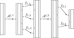
Figure 5: Realization of an example catalog network.

Our goal is to show that catalog networks can efficiently be approximated with neural networks with respect to some weight function, by which we mean any function $w\colon[0,\infty)\rightarrow(0,\infty)$.

Definition 7.

We say the decay of a weight function $w$ is controlled by $({s_{1}},{s_{2}})\in[1,\infty)\times[0,\infty)$ if

$${s_{1}}r^{{s_{2}}}w(r\max\{x,1\})\geq w(x)$$

for all $x\in[0,\infty)$ and $r\in[1,\infty)$.

Controlled decay is a general concept applicable to different types of weight functions. The inequality in Definition 7 is exactly what is needed in the proofs of our results. Useful weight functions are constants and functions of the form $(1+x^{q})^{-1}$ or $(\max\{1,x^{q}\})^{-1}$ for some $q\in(0,\infty)$. Constant weight functions have decay controlled by $(1,0)$. The functions $(1+x^{q})^{-1}$ and $(\max\{1,x^{q}\})^{-1}$ are covered by the following result.

Lemma 8.

Let $\delta\in(0,\infty)$ and consider a non-decreasing function $f\colon[0,\infty)\rightarrow(0,\infty)$. Moreover, let $g\colon[0,\infty)\rightarrow[0,\infty)$ be of the form $x\mapsto\mathop{\textstyle{\sum}}_{j=0}^{q}a_{j}x^{b_{j}}$ for $q\in\mathbb{N}_{0}=\mathbb{N}\cup\{0\}$ and $a_{0},b_{0},\dots,a_{q},b_{q}\in[0,\infty)$. Then the decay of the weight function $w(x)=f(x)(\max\{g(x),\delta\})^{-1}$ is controlled by $(\max\{g(1)/\delta,1\},\max\{b_{0},\dots,b_{q}\})$.

Our main interest is in catalogs of functions that are well approximable with neural networks. For the proofs of our main results to work we need the approximations to be Lipschitz continuous with a Lipschitz constant independent of the accuracy. To make this precise, we denote the Euclidean norm by $\|\cdot\|$.

Definition 9.

Consider an activation function $a\in C(\mathbb{R},\mathbb{R})$ and a weight function $w$. Fix constants $L\in[0,\infty)$ and $\varepsilon\in(0,1]$. Given a function $f\in\bigcup_{m,n\in\mathbb{N}}C(\mathbb{R}^{m},\mathbb{R}^{n})$ and a set $Q\subseteq\mathbb{R}^{\mathcal{I}(f)}$, we define the approximation cost $\mathrm{Cost}_{a,w}(f,Q,L,\varepsilon)$ as the infimum of the set

$$\left\{\mathcal{P}(\phi)\in\mathbb{N}\colon\begin{array}[]{cc}\phi\in\mathcal{N}\text{ with }\mathcal{R}_{a}^{\phi}\in C(\mathbb{R}^{\mathcal{I}(f)},\mathbb{R}^{\mathcal{O}(f)})\\ \text{s.t. }\mathcal{R}_{a}^{\phi}\text{ is }L\text{-Lipschitz on }\mathbb{R}^{\mathcal{I}(f)}\text{ and}\\ \sup_{x\in Q}w(\|x\|)\|f(x)-\mathcal{R}_{a}^{\phi}(x)\|\leq\varepsilon\end{array}\right\},$$

where, as usual, $\inf(\emptyset)$ is understood as $\infty$.

The next definition specifies the class of catalogs for which we will be able to prove Theorem 19 on the approximability of catalog networks.

Definition 10.

Let $a\in C(\mathbb{R},\mathbb{R})$, $\kappa=(\kappa_{0},\kappa_{1},\kappa_{2},\kappa_{3})\in[1,\infty)^{2}\times[0,\infty)^{2}$, $\varepsilon\in(0,1]$, and suppose $w$ is a weight function. Consider a subset $\mathcal{F}\subseteq\bigcup_{m,n\in\mathbb{N}}C(\mathbb{R}^{m},\mathbb{R}^{n})$ together with a family of sets $Q=(Q_{f})_{f\in\mathcal{F}}$ such that $Q_{f}\subseteq\mathbb{R}^{\mathcal{I}(f)}$ contains $0$ for all $f\in{\cal F}$ and a collection of Lipschitz constants $L=(L_{f})_{f\in\mathcal{F}}\subseteq[0,\infty)$. Then we call $\mathcal{F}$ an $[a,w,Q,L,\varepsilon,\kappa]$-approximable catalog if $\sup_{f\in\mathcal{F}}\|f(0)\|\leq\kappa_{0}$ and

$$\mathrm{Cost}_{a,w}(f,Q_{f},L_{f},\delta)\leq\kappa_{1}\max\{\mathcal{I}(f),\mathcal{O}(f)\}^{\kappa_{2}}\delta^{-\kappa_{3}}$$

for all $f\in\mathcal{F}$ and $\delta\in(0,\varepsilon]$.

Note that if $\mathcal{F}$ is $[a,w,Q,L,\varepsilon,\kappa]$-approximable, then every $f\in\mathcal{F}$ must be $L_{f}$-Lipschitz continuous on the set $Q_{f}$. Indeed, the definition implies that for all $\delta\in(0,\varepsilon]$ there exists $\phi_{\delta}\in\mathcal{N}$ such that $w(\|x\|)\|f(x)-\mathcal{R}_{a}^{\phi_{\delta}}(x)\|\leq\delta$ and $\|\mathcal{R}_{a}^{\phi_{\delta}}(x)-\mathcal{R}_{a}^{\phi_{\delta}}(y)\|\leq L_{f}\|x-y\|$ for all $x,y\in Q_{f}$. Hence, one obtains from the triangle inequality that

$$\|f(x)-f(y)\|\leq\frac{\delta}{w(\|x\|)}+L_{f}\|x-y\|+\frac{\delta}{w(\|y\|)}$$

for all $x,y\in Q_{f}$ and $\delta>0$, which shows that $f$ is $L_{f}$-Lipschitz on $Q_{f}$.

If ${\cal F}$ is a catalog approximable on sets $Q=(Q_{f})_{f\in\mathcal{F}}$ with Lipschitz constants $L=(L_{f})_{f\in\mathcal{F}}\subseteq[0,\infty)$, we define for a catalog network $\xi\in\mathcal{C}_{\mathcal{F}}^{l_{0},\dots,l_{2D}}$ of the form $\xi=[(V_{1},b_{1},\allowbreak(f_{1,1},\dots,f_{1,n_{1}})),\allowbreak\dots,\allowbreak(V_{D},b_{D},\allowbreak(f_{D,1},\dots,f_{D,n_{D}}))]$,

$$Q^{\xi,k}=\mathop{\textstyle{\prod}}_{j=1}^{n_{k}}Q_{f_{k,j}}\subseteq\mathop{\textstyle{\prod}}_{j=1}^{n_{k}}\mathbb{R}^{\mathcal{I}(f_{k,j})}=\mathbb{R}^{l_{2k-1}}$$

and

$$L^{\xi,k}=\max_{j\in\{1,\dots,n_{k}\}}L_{f_{k,j}}$$

for all $k\in\{1,\dots,\mathcal{D}_{\xi}\}$. Then the following holds.

Lemma 11.

Let $\xi\in\mathcal{C}_{\mathcal{F}}$ be a catalog network based on an $[a,w,Q,L,\varepsilon,\kappa]$-approximable catalog $\mathcal{F}$. Then

$$\|\mathcal{G}^{\xi,k}(x)-\mathcal{G}^{\xi,k}(y)\|\leq L^{\xi,k}\|x-y\|$$

for all $k\in\{1,\dots,\mathcal{D}_{\xi}\}$ and $x,y\in Q^{\xi,k}$.

IV Examples of Approximable Catalogs

In this section, we provide different examples of approximable catalogs that will be used in Section VII to show that various high-dimensional functions admit neural network approximations without the curse of dimensionality. Our catalogs are based on one-dimensional Lipschitz functions, the maximum function, the square, the product and the decreasing exponential function. They will be collected in Examples 12, 13, 15 and 17.

First, consider a $K$-Lipschitz function $f\colon\mathbb{R}\rightarrow\mathbb{R}$ for a constant $K\in[0,\infty)$. For any given $r\in(0,\infty)$, $f$ can be approximated on $[-r,r]$ with a piece-wise linear function supported on $N+1$ equidistributed points with accuracy $Kr/N$. Such a piece-wise linear function can be realized with a ReLU network $\phi_{N}$ with one hidden layer and $N$ hidden neurons. This results in $\mathcal{P}(\phi_{N})=3N+1$, from which it follows that

$$\mathrm{Cost}_{\mathrm{ReLU},1}(f,[-r,r],K,\varepsilon)\leq\mathcal{P}(\phi_{\lceil Kr\varepsilon^{-1}\rceil})\leq 3Kr\varepsilon^{-1}+4.$$

Alternatively, one can approximate $f$ on the entire real line with respect to a weight function of the form $w_{q}(x)=(1+x^{q})^{-1}$ for some $q\in(1,\infty)$. Then

$$\mathrm{Cost}_{\mathrm{ReLU},w_{q}}(f,\mathbb{R},K,\varepsilon)\leq 2^{\nicefrac{{1}}{{q-1}}}3(K\varepsilon^{-1})^{\nicefrac{{q}}{{q-1}}}+4,$$

the proof of which is a variant of [HutzJenKruseNguyen2020, Corollary 3.13]. Indeed, set $r=(2K\varepsilon^{-1})^{\nicefrac{{1}}{{(q-1)}}}$ and $N=\lceil Kr\varepsilon^{-1}\rceil$. Using $\phi_{N}$ as above, we have $|f(x)-\phi_{N}(x)|\leq\varepsilon$ for all $x\in[-r,r]$ and $|f(x)-\phi_{N}(x)|\leq 2K|x|$ for all $x\in\mathbb{R}\backslash[-r,r]$. The choice of $r$ then ensures that $w_{q}(|x|)|f(x)-\phi_{N}(x)|\leq\varepsilon$ for all $x\in\mathbb{R}$. In the notation of approximable catalogs, we can summarize as follows.

Example 12.

Let $r\in(0,\infty)$ and consider the weight function $w_{q}(x)=(1+x^{q})^{-1}$ for a $q\in(1,\infty)$. For $K\in[1,\infty)$, introduce the $K$-Lipschitz catalog

$$\begin{split}\mathcal{F}_{K}^{\mathrm{Lip}}=\big{\{}f\in C(\mathbb{R},\mathbb{R})\colon&f\text{ is }K\text{-Lipschitz}\text{ and }|f(0)|\leq K\big{\}}.\end{split}$$

Set $L_{\mathrm{id}_{\mathbb{R}}}=1$ and $L_{f}=K$ for $f\in\mathcal{F}_{K}^{\mathrm{Lip}}\backslash\{\mathrm{id}_{\mathbb{R}}\}$. If we define approximation sets by $Q_{\mathrm{id}_{\mathbb{R}}}=\mathbb{R}$ and

1. $Q_{f}=[-r,r]$ for all $f\in\mathcal{F}_{K}^{\mathrm{Lip}}\backslash\{\mathrm{id}_{\mathbb{R}}\}$, then $\mathcal{F}_{K}^{\mathrm{Lip}}$ is a $[\mathrm{ReLU},1,Q,L,1,\kappa]$-approximable catalog for $\kappa=(K,3Kr+4,0,1)$

2. $Q_{f}=\mathbb{R}$ for all $f\in\mathcal{F}_{K}^{\mathrm{Lip}}\backslash\{\mathrm{id}_{\mathbb{R}}\}$, then $\mathcal{F}_{K}^{\mathrm{Lip}}$ is a $[\mathrm{ReLU},w_{q},Q,L,1,\kappa]$-approximable catalog for $\kappa=(K,5(2K)^{\nicefrac{{q}}{{(q-1)}}},0,\nicefrac{{q}}{{q-1}})$.

Let us now turn to the maximum functions $\mathrm{max}_{d}\colon\mathbb{R}^{d}\rightarrow\mathbb{R},~{}x\mapsto\max\{x_{1},\dots,x_{d}\}$, $d\in\mathbb{N}$. They admit an exact representation with ReLU networks. Indeed, $\mathrm{max}_{1}$ is simply the identity and $\mathrm{max}_{2}$ is the ReLU-realization of

$$\phi_{2}=\left[\left(\begin{bmatrix}1&-1\\ 0&1\\ 0&-1\end{bmatrix},\begin{bmatrix}0\\ 0\\ 0\end{bmatrix}\right),\big{(}\begin{bmatrix}1&1&-1\end{bmatrix},0\big{)}\right]\!.$$

If $I\in\mathcal{N}$ is a skeleton for which ReLU satisfies the 2-identity requirement and we define $I_{d}=p(I,\dots,I)$, $d\in\mathbb{N}$, then it easily follows by induction that $\mathrm{max}_{d}$, $d\in\mathbb{N}_{\geq 3}$, is the ReLU-realization of $\phi_{d}=\phi_{d-1}\circ p(\phi_{2},I_{d-2})$, whose architecture is $(d,2d-1,2d-3,\dots,3,1)$. From this, we obtain $\mathcal{P}(\phi_{d})=\frac{1}{3}(4d^{3}+3d^{2}-4d+3)\leq 2d^{3}$. In other words, for all $d\in\mathbb{N}$ and any weight function $w$,

$$\mathrm{Cost}_{\mathrm{ReLU},w}(\mathrm{max}_{d},\mathbb{R}^{d},1,\varepsilon)\leq 2d^{3}.$$

Adding the maximum functions to the Lipschitz catalog, we obtain the following.

Example 13.

Adopt the setting of Example 12 and define the $K$-Lipschitz-maximum catalog $\mathcal{F}_{K}^{\mathrm{Lip,max}}=\mathcal{F}_{K}^{\mathrm{Lip}}\cup\{\mathrm{max}_{d}\colon d\in\mathbb{N}\}$. Add the approximation set $Q_{\mathrm{max}_{d}}=\mathbb{R}^{d}$ and the Lipschitz constant $L_{\mathrm{max}_{d}}=1$ for all $d\in\mathbb{N}$. Then $\mathcal{F}_{K}^{\mathrm{Lip,max}}$ is

1. a $[\mathrm{ReLU},1,Q,L,1,\kappa]$-approximable catalog for $\kappa=(K,3Kr+4,3,1)$ and $Q$ as in Example 12.(1).

2. a $[\mathrm{ReLU},w_{q},Q,L,1,\kappa]$-approximable catalog for $\kappa=(K,5(2K)^{\nicefrac{{q}}{{(q-1)}}},3,\nicefrac{{q}}{{q-1}})$ and $Q$ as in Example 12.(2).

Next, we study the approximability of the square function $\mathrm{sq}\colon\mathbb{R}\rightarrow\mathbb{R},~{}x\mapsto x^{2}$ . It has been shown by different authors that it can be approximated with accuracy $\varepsilon>0$ on the unit interval by the ReLU-realization of a skeleton $\phi_{\varepsilon}\in{\cal N}$ satisfying $\mathcal{P}(\phi_{\varepsilon})=\mathcal{O}(\log_{2}(\varepsilon^{-1}))$; see [Yarotsky2017, SchwabZech2019, GrohsHorJenZimm2019, GrohsPerekElbBolc2019]. A precise estimate of the required number of parameters is given in Proposition 3.3 of [GrohsHorJenZimm2019]. In our language it can be stated as

$$\mathrm{Cost}_{\mathrm{ReLU},1}(\mathrm{sq},[0,1],2,\varepsilon)\leq\max\{13,10\log_{2}(\varepsilon^{-1})-7\}.$$

Moreover, the neural network $\mathcal{R}_{\mathrm{ReLU}}^{\phi_{\varepsilon}}$ achieving this cost is 2-Lipschitz and satisfies $\mathcal{R}_{\mathrm{ReLU}}^{\phi_{\varepsilon}}=\mathrm{ReLU}$ on $\mathbb{R}\backslash[0,1]$. Using a mirroring and scaling argument, we can deduce the following estimate for approximating the square function on the interval $[-r,r]$ for any $r\in(0,\infty)$.

Lemma 14.

For all $r\in(0,\infty)$ and $\varepsilon\in(0,1]$, there exists a skeleton $\psi_{r,\varepsilon}\in\mathcal{N}$ such that $\mathcal{R}_{\mathrm{ReLU}}^{\psi_{r,\varepsilon}}\in C(\mathbb{R},\mathbb{R})$ is $2r$-Lipschitz, $\sup_{x\in[-r,r]}|\mathcal{R}_{\mathrm{ReLU}}^{\psi_{r,\varepsilon}}(x)-x^{2}|\leq\varepsilon$, $\mathcal{R}_{\mathrm{ReLU}}^{\psi_{r,\varepsilon}}(x)=r|x|$ for all $x\in\mathbb{R}\backslash[-r,r]$ and

$$\mathcal{P}(\psi_{r,\varepsilon})\leq\max\{52,80\log_{2}(r)+40\log_{2}(\varepsilon^{-1})-28\}.$$

More concisely, for all $r\in[2,\infty)$ and $\varepsilon\in(0,1]$, the statement of Lemma 14 can be written as

$$\begin{split}\mathrm{Cost}_{\mathrm{ReLU},1}(\mathrm{sq},[-r,r],2r,\varepsilon)&\leq\\ 80\log_{2}(r)&+40\log_{2}(\varepsilon^{-1})-28.\end{split}$$

Now, let us take a closer look at the decreasing exponential function $\mathrm{e}\colon\mathbb{R}\rightarrow\mathbb{R},~{}x\mapsto e^{-x}$. Its restriction to $[0,\infty)$ is covered by the general approximation result for Lipschitz functions. But exploiting its exponential decrease, we can obtain better estimates. More precisely, $\mathrm{e}$ can be approximated to a given accuracy $\varepsilon\in(0,1]$ uniformly on $[0,\infty)$ with a piece-wise linear interpolation supported on the $\lfloor\varepsilon^{-1}\rfloor$ points $-\log(n\varepsilon)$, $n\in\{1,\dots,\lfloor\varepsilon^{-1}\rfloor\}$ which is constant on $\mathbb{R}\backslash[-\log(\lfloor\varepsilon^{-1}\rfloor\varepsilon),-\log(\varepsilon)]$. Realizing this piece-wise linear function with a ReLU network with one hidden layer yields

$$\mathrm{Cost}_{\mathrm{ReLU},1}(\mathrm{e},[0,\infty),1,\varepsilon)\leq 3\lfloor\varepsilon^{-1}\rfloor+1\leq 4\varepsilon^{-1}.$$

Together with $\mathrm{id}_{\mathbb{R}}$ and $\mathrm{sq}$, $\mathrm{e}$ gives rise to the following catalog, which we will use to approximate generalized Gaussian radial basis function networks in Section VII.

Example 15.

Let $r\in[5,\infty)$. Define the catalog $\mathcal{F}^{\mathrm{RBF}}=\{\mathrm{id}_{\mathbb{R}},\mathrm{e},\mathrm{sq}\}$ with approximation sets $Q_{\mathrm{id}_{\mathbb{R}}}=\mathbb{R}$, $Q_{\mathrm{e}}=[0,\infty)$, $Q_{\mathrm{sq}}=[-r,r]$ and Lipschitz constants $L_{\mathrm{id}_{\mathbb{R}}}=L_{\mathrm{e}}=1$, $L_{\mathrm{sq}}=2r$. Then $\mathcal{F}^{\mathrm{RBF}}$ is a $[\mathrm{ReLU},1,Q,L,r^{-3},(1,4,0,1)]$-approximable catalog.

Using the identity $xy=\frac{1}{4}((x+y)^{2}-(x-y)^{2})$, we can also estimate the approximation rate of the product function $\mathrm{pr}\colon\mathbb{R}^{2}\rightarrow\mathbb{R},~{}(x,y)\mapsto xy$. This trick has already been used before by, e.g., [Yarotsky2017, LinTegRol2017]. We still provide a proof of the following proposition since the results in the existing literature do not specify the Lipschitz constant. Our proofs of both, Lemma 14 and Proposition 16, follow the reasoning of Section 3 in [GrohsHorJenZimm2019].

Proposition 16.

For all $r\in(0,\infty)$ and $\varepsilon\in(0,\frac{1}{2}]$, one has

$$\begin{split}\mathrm{Cost}_{\mathrm{ReLU},1}(\mathrm{pr},[-r,r]^{2},\sqrt{8}r,\varepsilon)&\leq\\ \max\{208,320\log_{2}(r)&+160\log_{2}(\varepsilon^{-1})+48\}.\end{split}$$

The following is our last example of an approximable catalog.

Example 17.

Take $\mathcal{F}_{K}^{\mathrm{Lip}}$ from Example 12, let $R\in(0,\infty)$, and define the $K$-Lipschitz-product catalog $\mathcal{F}_{K}^{\mathrm{Lip,prod}}=\mathcal{F}_{K}^{\mathrm{Lip}}\cup\{\mathrm{pr}\}$. The approximation sets and Lipschitz constants are defined as in (1) of Example 12 for $\mathcal{F}_{K}^{\mathrm{Lip}}$ and $Q_{\mathrm{pr}}=[-R,R]^{2}$, $L_{\mathrm{pr}}=\sqrt{8}R$. Then $\mathcal{F}_{K}^{\mathrm{Lip,prod}}$ is a $[\mathrm{ReLU},1,Q,L,\delta,(K,M,0,1)]$-approximable catalog for $\delta=\min\{\nicefrac{{1}}{{2}},\nicefrac{{R^{2}}}{{2}}\}$ and $M=\max\{3Kr+4,105R^{2}\}$.

V Approximation Results

In this section, we state the first of our main results, Theorem 19, on the approximability of catalog networks with neural networks and explore the special case of ReLU activation in Corollaries 22 and 23. The next lemma is crucial for the proof of Theorem 19. It establishes the approximability of the functions $\mathcal{G}^{\xi,k}$, $k\in\{1,\dots,\mathcal{D}_{\xi}\}$, in a catalog network $\xi\in\mathcal{C}_{\mathcal{F}}$. Since $\mathcal{G}^{\xi,k}$ is composed of functions $f_{k,1},\dots,f_{k,n_{k}}$ from the catalog $\mathcal{F}$, it can be approximated by approximating $f_{k,1},\dots,f_{k,n_{k}}$ with neural networks and then parallelizing them as in Figure 3. Proposition 5 allows us to keep track of the resulting number of parameters.

Lemma 18.

Assume $a\in C(\mathbb{R},\mathbb{R})$ satisfies the $c$-identity requirement for some $c\geq 2$. Let $\mathcal{F}$ be an $[a,w,Q,L,\varepsilon,\kappa]$-approximable catalog for a non-increasing weight function $w$, and consider a catalog network $\xi\in\mathcal{C}_{\mathcal{F}}^{l_{0},\dots,l_{2D}}$ for some $D\in\mathbb{N}$ and $l_{0},\dots,l_{2D}\in\mathbb{N}$. Then for all $k\in\{1,\dots,D\}$ and $\delta\in(0,\varepsilon]$, there exists a skeleton $\phi\in\mathcal{N}$ with $a$-realization $\mathcal{R}_{a}^{\phi}\in C(\mathbb{R}^{l_{2k-1}},\mathbb{R}^{l_{2k}})$ such that

1. $\sup_{x\in Q^{\xi,k}}w(\|x\|)\|\mathcal{G}^{\xi,k}(x)-\mathcal{R}_{a}^{\phi}(x)\|\leq\delta$,

2. $\mathcal{R}_{a}^{\phi}$ is $L^{\xi,k}$-Lipschitz continuous on $\mathbb{R}^{l_{2k-1}}$ and

3. $\mathcal{P}(\phi)\leq\frac{11}{16}\kappa_{1}c^{2}\max\{l_{2k-1},l_{2k}\}^{\kappa_{2}+\kappa_{3}/2+5}\delta^{-\kappa_{3}}$.

If, in addition, $\mathcal{I}(f)\leq d$ and $\mathcal{O}(f)\leq d$ for some $d\in\mathbb{N}$ and all $f\in\mathcal{F}$, then one also has

1. $\mathcal{P}(\phi)\leq\frac{11}{16}\kappa_{1}c^{2}d^{2}\max\{l_{2k-1},l_{2k}\}^{\kappa_{2}+\kappa_{3}/2+3}\delta^{-\kappa_{3}}$.

Before we can formulate Theorem 19, we have to introduce a few more concepts. Let $\mathcal{F}$ be a catalog that is approximable on sets $Q=(Q_{f})_{f\in\mathcal{F}}$ with Lipschitz constants $L=(L_{f})_{f\in\mathcal{F}}\subseteq[0,\infty)$. Then, for any catalog network $\xi=[(V_{1},b_{1},\allowbreak(f_{1,1},\dots,f_{1,n_{1}})),\allowbreak\dots,\allowbreak(V_{D},b_{D},\allowbreak(f_{D,1},\dots,f_{D,n_{D}}))]\in\mathcal{C}_{\mathcal{F}}$, we define

$$\begin{split}&\mathrm{Dom}_{Q,\xi}=\bigg{\{}x\in\mathbb{R}^{\mathcal{I}_{\xi}}\colon\text{for all }k\in\{1,\dots,\mathcal{D}_{\xi}\}\colon\\ &\big{(}\mathcal{A}^{\xi,k}\circ\mathcal{G}^{\xi,k-1}\circ\cdots\circ\mathcal{A}^{\xi,2}\circ\mathcal{G}^{\xi,1}\circ\mathcal{A}^{\xi,1}\big{)}(x)\in Q^{\xi,k}\bigg{\}}\end{split}$$

and

$$\mathrm{Lip}_{L,\xi}=\prod_{k=1}^{\mathcal{D}_{\xi}}L^{\xi,k}\|V_{k}\|,$$

where $\|\cdot\|$ denotes the operator norm when applied to matrices. The set $\mathrm{Dom}_{Q,\xi}$ describes where we will be able to approximate the catalog network $\xi$. It takes into account that each each layer function $\mathcal{G}^{\xi,k}$ can only be approximated on the set $Q^{\xi,k}$. The number $\mathrm{Lip}_{L,\xi}$ represents the worst-case Lipschitz constant of the catalog network.

To estimate the approximation error, we need two more quantities. The first one is

$$\mathcal{B}_{\xi}=\max\big{\{}1,\|\mathcal{A}^{\xi,1}(0)\|,\dots,\|\mathcal{A}^{\xi,\mathcal{D}_{\xi}}(0)\|\big{\}},$$

which simply measures the maximal norm of the inhomogeneous parts of the affine transformations (capped from below by 1). When using weight functions of the type $w_{q}(x)=(1+x^{q})^{-1}$, functions in the catalog are approximated better close to the origin. The quantity $\mathcal{B}_{\xi}$ together with the $\kappa_{0}$-boundedness of the catalog in the origin will be used to control how far away one is from the region where one has the best approximation. However, this becomes irrelevant for constant weight functions, as can be seen in Corollary 23 below.

The last quantity we need is $\mathcal{T}_{L,\xi}$, defined as the maximum of 1 and

$$\max_{k\in\{0,\dots,D-1\}}\max\{1,L^{\xi,k},L^{\xi,D}\}\|V_{D}\|\prod_{j=k+1}^{D-1}L^{\xi,j}\|V_{j}\|$$

where we abbreviate $D=\mathcal{D}_{\xi}$ and use the convention $L^{\xi,0}=0$. This combines the Lipschitz constants of the affine and nonlinear functions appearing in the different layers of the catalog network $\xi$.

Theorem 19.

Suppose $a\in C(\mathbb{R},\mathbb{R})$ fulfills the $c$-identity requirement for some number $c\geq 2$ and let $w$ be a non-increasing weight function whose decay is controlled by $({s_{1}},{s_{2}})$ for some ${s_{1}}\in[1,\infty)$ and ${s_{2}}\in[0,\infty)$. Consider a catalog network $\xi\in\mathcal{C}_{\mathcal{F}}$ for an $[a,w,Q,L,\varepsilon,\kappa]$-approximable catalog $\mathcal{F}$. Then there exists a skeleton $\phi\in\mathcal{N}$ with $a$-realization $\mathcal{R}_{a}^{\phi}\in C(\mathbb{R}^{\mathcal{I}_{\xi}},\mathbb{R}^{\mathcal{O}_{\xi}})$ such that

1. $\sup_{x\in\mathrm{Dom}_{Q,\xi}}w(\|x\|)\|\mathcal{R}^{\xi}(x)-\mathcal{R}_{a}^{\phi}(x)\|\leq\varepsilon$,

2. $\mathcal{R}_{a}^{\phi}$ is $\mathrm{Lip}_{L,\xi}$-Lipschitz continuous on $\mathbb{R}^{\mathcal{I}_{\xi}}$ and

3. $\mathcal{P}(\phi)\leq C\mathcal{B}_{\xi}^{t-\kappa_{3}}\mathcal{T}_{L,\xi}^{t}\mathcal{D}_{\xi}^{t+1}\mathcal{W}_{\xi}^{\kappa_{2}+t/2+6}\varepsilon^{-\kappa_{3}}$
   for $t=\kappa_{3}({s_{2}}+1)$ and $C=\tfrac{81}{32}c^{3}(4\kappa_{0})^{t-\kappa_{3}}\kappa_{1}{s_{1}}^{\kappa_{3}}$.

The conclusion of Theorem 19 could be written more concisely as

$$\begin{split}\mathrm{Cost}_{a,w}(\mathcal{R}^{\xi},&\,\mathrm{Dom}_{Q,\xi},\mathrm{Lip}_{L,\xi},\varepsilon)\\ &\leq C\mathcal{B}_{\xi}^{t-\kappa_{3}}\mathcal{T}_{L,\xi}^{t}\mathcal{D}_{\xi}^{t+1}\mathcal{W}_{\xi}^{\kappa_{2}+t/2+6}\varepsilon^{-\kappa_{3}}.\end{split}$$

We point out that the rate in the accuracy is $\mathcal{O}(\varepsilon^{-\kappa_{3}})$, the same as for the underlying catalog $\mathcal{F}$.

In the proof of Theorem 19, we combine the approximations of the functions $\mathcal{G}^{\xi,k}$ obtained in Lemma 18 with the affine maps $\mathcal{A}^{\xi,k}$. When concatenating different approximating networks, we interpose identity networks. This reduces the parameter count in worst-case scenarios but can lead to slightly looser estimates in certain other situations.

Remark 20.

If $\mathcal{I}(f)\leq d$ and $\mathcal{O}(f)\leq d$ for some $d\in\mathbb{N}$ and all $f\in\mathcal{F}$, we can use (4) instead of (3) of Lemma 18 in the proof of Theorem 19 to obtain the following modified version of the parameter bound in Theorem 19:

$$\mathcal{P}(\phi)\leq Cd^{2}\mathcal{B}_{\xi}^{t-\kappa_{3}}\mathcal{T}_{L,\xi}^{t}\mathcal{D}_{\xi}^{t+1}\mathcal{W}_{\xi}^{\kappa_{2}+t/2+4}\varepsilon^{-\kappa_{3}}.$$

Since in many of the example catalogs of Section IV, the maximal input/output dimension is 1 or 2, this will allow us to obtain better estimates in some of the applications in Section VII below.

Remark 21.

A careful inspection of the proof of Theorem 19 shows that it does not only work for the Euclidean norm but also, for instance, the sup-norm.

We know that the ReLU activation function satisfies the 2-identity requirement. Theorem 19 recast for ReLU activation and the weight function $w_{q}(x)=(1+x^{q})^{-1}$ reads as follows:

Corollary 22.

Consider the weight function $w_{q}(x)=(1+x^{q})^{-1}$ for some $q\in(0,\infty)$. Let $\xi\in\mathcal{C}_{\mathcal{F}}$ be a catalog network for a $[\mathrm{ReLU},w_{q},Q,L,\varepsilon,\kappa]$-approximable catalog $\mathcal{F}$. Then there exists a skeleton $\phi\in\mathcal{N}$ with ReLU-realization $\mathcal{R}_{\mathrm{ReLU}}^{\phi}\in C(\mathbb{R}^{\mathcal{I}_{\xi}},\mathbb{R}^{\mathcal{O}_{\xi}})$ such that

1. $\sup_{x\in\mathrm{Dom}_{Q,\xi}}(1+\|x\|^{q})^{-1}\|\mathcal{R}^{\xi}(x)-\mathcal{R}_{\mathrm{ReLU}}^{\phi}(x)\|\leq\varepsilon$,

2. $\mathcal{R}_{\mathrm{ReLU}}^{\phi}$ is $\mathrm{Lip}_{L,\xi}$-Lipschitz continuous on $\mathbb{R}^{\mathcal{I}_{\xi}}$ and

3. $\mathcal{P}(\phi)\leq C\mathcal{B}_{\xi}^{t-\kappa_{3}}\mathcal{T}_{L,\xi}^{t}\mathcal{D}_{\xi}^{t+1}\mathcal{W}_{\xi}^{\kappa_{2}+t/2+6}\varepsilon^{-\kappa_{3}}$
   for $t=\kappa_{3}(q+1)$ and $C=\tfrac{81}{4}2^{2t-\kappa_{3}}\kappa_{0}^{t-\kappa_{3}}\kappa_{1}$.

For the weight function $w\equiv 1$, the parameter estimate in Theorem 19 simplifies considerably. This is because the decay of $w\equiv 1$ is controlled by $(1,0)$, which makes the translation size and the bound of the catalog in the origin irrelevant.

Corollary 23.

Let $\xi\in\mathcal{C}_{\mathcal{F}}$ be a catalog network for a $[\mathrm{ReLU},1,Q,L,\varepsilon,\kappa]$-approximable catalog $\mathcal{F}$. Then there exists a skeleton $\phi\in\mathcal{N}$ with ReLU-realization $\mathcal{R}_{\mathrm{ReLU}}^{\phi}\in C(\mathbb{R}^{\mathcal{I}_{\xi}},\mathbb{R}^{\mathcal{O}_{\xi}})$ such that

1. $\sup_{x\in\mathrm{Dom}_{Q,\xi}}\|\mathcal{R}^{\xi}(x)-\mathcal{R}_{\mathrm{ReLU}}^{\phi}(x)\|\leq\varepsilon$,

2. $\mathcal{R}_{\mathrm{ReLU}}^{\phi}$ is $\mathrm{Lip}_{L,\xi}$-Lipschitz continuous on $\mathbb{R}^{\mathcal{I}_{\xi}}$ and

3. $\mathcal{P}(\phi)\leq\tfrac{81}{4}\kappa_{1}\mathcal{T}_{L,\xi}^{\kappa_{3}}\mathcal{D}_{\xi}^{\kappa_{3}+1}\mathcal{W}_{\xi}^{\kappa_{2}+\kappa_{3}/2+6}\varepsilon^{-\kappa_{3}}$.

VI Log-approximable Catalogs

In this section, we modify the way we measure the approximation cost and derive corresponding approximation results.

Definition 24.

With the setup of Definition 10 and $\varepsilon\leq 1/2$, a subset $\mathcal{F}\subseteq\bigcup_{m,n\in\mathbb{N}}C(\mathbb{R}^{m},\mathbb{R}^{n})$ is called $[a,w,Q,L,\varepsilon,\kappa]$-log-approximable if $\sup_{f\in\mathcal{F}}\|f(0)\|\leq\kappa_{0}$ and

$$\mathrm{Cost}_{a,w}(f,Q_{f},L_{f},\delta)\leq\kappa_{1}\!\max\{\mathcal{I}(f),\mathcal{O}(f)\}^{\!\kappa_{2}}[\log_{2}(\delta^{-1})]^{\kappa_{3}}$$

for all $f\in\mathcal{F}$ and $\delta\in(0,\varepsilon]$.

This log-modification is designed for catalogs made of functions like the square or the product, which can be approximated with rate $\mathcal{O}(\log_{2}(\varepsilon^{-1}))$, as we have seen in Lemmas 14 and 16. Its usefulness will become apparent in Proposition 33, which is based on the following catalog.

Example 25.

Let $\mathcal{F}^{\mathrm{prod}}=\{\mathrm{id}_{\mathbb{R}},\mathrm{pr}\}$ be the product catalog and fix $r\in[1,\infty)$ and $d\in\mathbb{N}$. Consider the approximation sets $Q_{\mathrm{id}_{\mathbb{R}}}=\mathbb{R}$, $Q_{\mathrm{pr}}=[-r^{d},r^{d}]^{2}$ and the Lipschitz constants $L_{\mathrm{id}_{\mathbb{R}}}=1$, $L_{\mathrm{pr}}=\sqrt{8}r^{d}$. Then $\mathcal{F}^{\mathrm{prod}}$ is a $[\mathrm{ReLU},1,Q,L,\min\{1/2,1/r\},(1,320d+208,0,1)]$-log-approximable catalog, where $\kappa_{1}$ can also be chosen as $208$ instead of $320d+208$ if $r=1$.

Using the notion of log-approximable catalogs, we can derive the following analogue of Theorem 19.

Theorem 26.

Assume $a\in C(\mathbb{R},\mathbb{R})$ satisfies the $c$-identity requirement for some number $c\geq 2$, and let $w$ be a non-increasing weight function whose decay is controlled by $({s_{1}},{s_{2}})$ for some ${s_{1}}\in[1,\infty)$ and ${s_{2}}\in[0,\infty)$. Consider a catalog network $\xi\in\mathcal{C}_{\mathcal{F}}$ for an $[a,w,Q,L,\varepsilon,\kappa]$-log-approximable catalog ${\cal F}$. Then there exists a skeleton $\phi\in\mathcal{N}$ with $a$-realization $\mathcal{R}_{a}^{\phi}\in C(\mathbb{R}^{\mathcal{I}_{\xi}},\mathbb{R}^{\mathcal{O}_{\xi}})$ such that

1. $\sup_{x\in\mathrm{Dom}_{Q,\xi}}w(\|x\|)\|\mathcal{R}^{\xi}(x)-\mathcal{R}_{a}^{\phi}(x)\|\leq\varepsilon$,

2. $\mathcal{R}_{a}^{\phi}$ is $\mathrm{Lip}_{L,\xi}$-Lipschitz continuous on $\mathbb{R}^{\mathcal{I}_{\xi}}$ and

3. $\mathcal{P}(\phi)\leq\tfrac{81}{32}c^{3}\kappa_{1}\mathcal{D}_{\xi}\mathcal{W}_{\xi}^{\kappa_{2}+6}$
   $\times\big{[}\!\log_{2}\!\big{(}{s_{1}}[4\kappa_{0}\mathcal{B}_{\xi}]^{{s_{2}}}[\mathcal{T}_{L,\xi}\mathcal{D}_{\xi}\sqrt{\mathcal{W}_{\xi}}]^{{s_{2}}+1}\varepsilon^{-1}\big{)}\big{]}^{\kappa_{3}}$.

The following is the analogue of Corollary 23 for log-approximable catalogs.

Corollary 27.

Let $\xi\in\mathcal{C}_{\mathcal{F}}$ be a catalog network for a $[\mathrm{ReLU},1,Q,L,\varepsilon,\kappa]$-log-approximable catalog $\mathcal{F}$. Then there exists a skeleton $\phi\in\mathcal{N}$ with ReLU-realization $\mathcal{R}_{\mathrm{ReLU}}^{\phi}\in C(\mathbb{R}^{\mathcal{I}_{\xi}},\mathbb{R}^{\mathcal{O}_{\xi}})$ such that

1. $\sup_{x\in\mathrm{Dom}_{Q,\xi}}\|\mathcal{R}^{\xi}(x)-\mathcal{R}_{\mathrm{ReLU}}^{\phi}(x)\|\leq\varepsilon$,

2. $\mathcal{R}_{\mathrm{ReLU}}^{\phi}$ is $\mathrm{Lip}_{L,\xi}$-Lipschitz continuous on $\mathbb{R}^{\mathcal{I}_{\xi}}$ and

3. $\mathcal{P}(\phi)\leq\tfrac{81}{4}\kappa_{1}\mathcal{D}_{\xi}\mathcal{W}_{\xi}^{\kappa_{2}+6}\big{[}\!\log_{2}\!\big{(}\mathcal{T}_{L,\xi}\mathcal{D}_{\xi}\sqrt{\mathcal{W}_{\xi}}\varepsilon^{-1}\big{)}\big{]}^{\kappa_{3}}$.

VII Overcoming the Curse of Dimensionality

In this section, we apply the theory of catalog networks to show that different high-dimensional functions admit a ReLU neural network approximation without the curse of dimensionality. We use the catalogs introduced in Sections IV and VI to construct families of functions indexed by the dimension of their domain that are of the same form for each dimension. The results in this section are proved by finding catalog network representations of the high-dimensional target functions, so that one of the general approximation results of Sections V or VI can be applied. The mere approximability of these functions with ReLU networks follows from classical universal approximation results such as [LeshnoLinPinkusScho1993]. But the quantitative estimates on the number of parameters in terms of the dimension $d$ and the accuracy $\varepsilon$ are new.

Our general results cover a wide range of interesting examples, but it is possible that, for some of them, the estimates could be improved by using their special structure.

Proposition 28.

Fix $K,r\in[1,\infty)$, and let $f_{i}\colon\mathbb{R}\rightarrow\mathbb{R}$, $i\in\mathbb{N}$, be $K$-Lipschitz continuous with $|f_{i}(0)|\leq K$. Define $g_{d}\colon\mathbb{R}^{d}\rightarrow\mathbb{R}$ by $g_{d}(x)=\mathop{\textstyle{\sum}}_{i=1}^{d}f_{i}(x_{i})$. Then for all $d\in\mathbb{N}$ and $\varepsilon\in(0,1]$, there exists $\phi\in\mathcal{N}$ with $\mathcal{R}_{\mathrm{ReLU}}^{\phi}\in C(\mathbb{R}^{d},\mathbb{R})$ such that

1. $\sup_{x\in[-r,r]^{d}}|g_{d}(x)-\mathcal{R}_{\mathrm{ReLU}}^{\phi}(x)|\leq\varepsilon$,

2. $\mathcal{R}_{\mathrm{ReLU}}^{\phi}$ is $\sqrt{d}K$-Lipschitz continuous on $\mathbb{R}^{d}$ and

3. $\mathcal{P}(\phi)\leq\tfrac{4}{7}10^{3}K^{2}rd^{5}\varepsilon^{-1}$.

The following is a generalization, whose proof only requires a slight adjustment.

Proposition 29.

Fix $K,r\in[1,\infty)$, and let $f_{i}\colon\mathbb{R}\rightarrow\mathbb{R}$, $i\in\mathbb{N}_{0}$, be $K$-Lipschitz continuous with $|f_{i}(0)|\leq K$. Define $g_{d}\colon\mathbb{R}^{d}\rightarrow\mathbb{R}$ by $g_{d}(x)=f_{0}(\mathop{\textstyle{\sum}}_{i=1}^{d}f_{i}(x_{i}))$. Then for all $d\in\mathbb{N}$ and $\varepsilon\in(0,1]$, there exists $\phi\in\mathcal{N}$ with $\mathcal{R}_{\mathrm{ReLU}}^{\phi}\in C(\mathbb{R}^{d},\mathbb{R})$ such that

1. $\sup_{x\in[-r,r]^{d}}|g_{d}(x)-\mathcal{R}_{\mathrm{ReLU}}^{\phi}(x)|\leq\varepsilon$,

2. $\mathcal{R}_{\mathrm{ReLU}}^{\phi}$ is $\sqrt{d}K^{2}$-Lipschitz continuous on $\mathbb{R}^{d}$ and

3. $\mathcal{P}(\phi)\leq\tfrac{5}{6}10^{3}K^{4}rd^{6}\varepsilon^{-1}$.

Note that the parameter estimates in Propositions 28 and 29 depend on $r$ since we approximate uniformly on the hypercube $[-r,r]^{d}$. However, the estimate is only linear in $r$, even though the volume of the hypercube is of the order $r^{d}$.

Proposition 30.

Let $K,r\in[1,\infty)$ and suppose $f_{i}\colon\mathbb{R}\rightarrow\mathbb{R}$ is $K$-Lipschitz with $|f_{i}(0)|\leq K$ and $g_{i}\colon\mathbb{R}\rightarrow\mathbb{R}$ 1-Lipschitz with $g_{i}(0)=0$, $i\in\mathbb{N}$. Let $h_{d}\colon\mathbb{R}^{d}\rightarrow\mathbb{R}$, $d\in\mathbb{N}$, be given by $h_{1}=f_{1}$ and $h_{d}(x)=g_{d}(\max\{h_{d-1}(x_{1},\dots,x_{d-1}),f_{d}(x_{d})\})$ for $d\geq 2$. Then for all $d\in\mathbb{N}$ and $\varepsilon\in(0,1]$, there exists $\phi\in\mathcal{N}$ with $\mathcal{R}_{\mathrm{ReLU}}^{\phi}\in C(\mathbb{R}^{d},\mathbb{R})$ such that

1. $\sup_{x\in[-r,r]^{d}}|h_{d}(x)-\mathcal{R}_{\mathrm{ReLU}}^{\phi}(x)|\leq\varepsilon$,

2. $\mathcal{R}_{\mathrm{ReLU}}^{\phi}$ is $K$-Lipschitz continuous on $\mathbb{R}^{d}$ and

3. $\mathcal{P}(\phi)\leq\frac{3}{7}10^{4}K^{3}rd^{\nicefrac{{13}}{{2}}}\varepsilon^{-1}$.

Note that if the functions $g_{i}$, for $1\leq i\leq d-1$, are chosen to be the identity and $g_{d}=f_{0}$, then $h_{d}$ reduces to $f_{0}(\max\{f_{1}(x_{1}),\dots,f_{d}(x_{d})\})$.

The functions in the previous propositions were approximated on bounded domains, but if one is willing to pay a higher approximation cost, one can also approximate the family of functions from, e.g., Proposition 28 on the entire space without the curse of dimensionality for an appropriate weight function.

Proposition 31.

Let $q\in(1,\infty)$, $K\in[1,\infty)$ and suppose $f_{i}\colon\mathbb{R}\rightarrow\mathbb{R}$, $i\in\mathbb{N}$, are $K$-Lipschitz continuous with $|f_{i}(0)|\leq K$. Define $g_{d}\colon\mathbb{R}^{d}\rightarrow\mathbb{R}$ by $g_{d}(x)=\mathop{\textstyle{\sum}}_{i=1}^{d}f_{i}(x_{i})$. Then for all $d\in\mathbb{N}$ and $\varepsilon\in(0,1]$, there exists $\phi\in\mathcal{N}$ with $\mathcal{R}_{\mathrm{ReLU}}^{\phi}\in C(\mathbb{R}^{d},\mathbb{R})$ such that

1. $\sup_{x\in\mathbb{R}^{d}}(1+\|x\|^{q})^{-1}|g_{d}(x)-\mathcal{R}_{\mathrm{ReLU}}^{\phi}(x)|\leq\varepsilon$,

2. $\mathcal{R}_{\mathrm{ReLU}}^{\phi}$ is $\sqrt{d}K$-Lipschitz continuous on $\mathbb{R}^{d}$ and

3. $\mathcal{P}(\phi)\leq\tfrac{2}{9}10^{3}2^{3t(q+1)}K^{2t(q+1)}d^{t(q+1)+4}\varepsilon^{-t}$
   for $t=\nicefrac{{q}}{{q-1}}$.

An analogous result with the maximum function instead of the sum can be shown similarly.

In the next two propositions, we replace the sum by a product. Then we cannot establish the approximation on an arbitrarily large domain since the Lipschitz constant of the product function on $[-r,r]^{2}$ grows linearly in $r$.

Proposition 32.

Let $K\in[1,\infty)$ and suppose $f_{i}\colon\mathbb{R}\rightarrow\mathbb{R}$ is $K$-Lipschitz and $g_{i}\colon\mathbb{R}\rightarrow\mathbb{R}$ 1-Lipschitz with $f_{i}(0)=0=g_{i}(0)$, $i\in\mathbb{N}$. Let $h_{d}\colon\mathbb{R}^{d}\rightarrow\mathbb{R}$, $d\in\mathbb{N}$, be given by $h_{1}=f_{1}$ and $h_{d}(x)=g_{d}(h_{d-1}(x_{1},\dots,x_{d-1})f_{d}(x_{d}))$ for $d\geq 2$. Set $r=\nicefrac{{1}}{{\sqrt{8}K}}$. Then for all $d\in\mathbb{N}$ and $\varepsilon\in(0,\nicefrac{{1}}{{16}}]$, there exists $\phi\in\mathcal{N}$ with $\mathcal{R}_{\mathrm{ReLU}}^{\phi}\in C(\mathbb{R}^{d},\mathbb{R})$ such that

1. $\sup_{x\in[-r,r]^{d}}|h_{d}(x)-\mathcal{R}_{\mathrm{ReLU}}^{\phi}(x)|\leq\varepsilon$,

2. $\mathcal{R}_{\mathrm{ReLU}}^{\phi}$ is $K$-Lipschitz continuous on $\mathbb{R}^{d}$ and

3. $\mathcal{P}(\phi)\leq\frac{3}{7}10^{4}K^{2}d^{\nicefrac{{13}}{{2}}}\varepsilon^{-1}$.

This example includes the special case $f_{0}(\prod_{i=1}^{d}f_{i}(x_{i}))$. Since on large hypercubes the quantity $\mathcal{T}_{L,\xi_{d}}$, where $\xi_{d}$ is a catalog network representing the function $h_{d}$, starts to grow exponentially in the dimension, the approximators in the proof of Proposition 32 can only be built on the hypercube $[-\nicefrac{{1}}{{\sqrt{8}K}},\nicefrac{{1}}{{\sqrt{8}K}}]^{d}$.

However, it has been shown in Proposition 3.3. of [SchwabZech2019] that the product $\prod_{i=1}^{d}x_{i}$ can be approximated without the curse of dimensionality on the hypercube $[-1,1]^{d}$. Applying the $\log$-modification of our theory, we can recover this result and even allow for arbitrarily large hypercubes.

Proposition 33.

Consider the functions $f_{d}\colon\mathbb{R}^{d}\rightarrow\mathbb{R}$, $d\in\mathbb{N}$, given by $f_{d}(x)=\prod_{i=1}^{d}x_{i}$, and let $r\in[1,\infty)$. Then for all $d\in\mathbb{N}_{\geq 2}$ and $\varepsilon\in(0,\min\{1/2,r^{-1}\}]$, there exists $\phi\in\mathcal{N}$ with $\mathcal{R}_{\mathrm{ReLU}}^{\phi}\in C(\mathbb{R}^{d},\mathbb{R})$ such that

1. $\sup_{x\in[-r,r]^{d}}|f_{d}(x)-\mathcal{R}_{\mathrm{ReLU}}^{\phi}(x)|\leq\varepsilon$,

2. $\mathcal{R}_{\mathrm{ReLU}}^{\phi}$ is $8^{\nicefrac{{(d-1)}}{{2}}}r^{d(d-1)}$-Lipschitz continuous on $\mathbb{R}^{d}$,

3. $\mathcal{P}(\phi)\leq\tfrac{1}{3}10^{5}\log_{2}(d)d^{6}\log_{2}(\varepsilon^{-1})$ if $r=1$ and

4. $\mathcal{P}(\phi)\leq\tfrac{2}{5}10^{5}\log_{2}(r)\log_{2}(d)d^{8}\log_{2}(\varepsilon^{-1})$ if $r\geq 2$.

In our next result, we show the approximability of ridge functions based on a Lipschitz function.

Proposition 34.

Let $K,r,S\in[1,\infty)$, $\theta_{d}\in[-S,S]^{d}$, $d\in\mathbb{N}$, and suppose $f\colon\mathbb{R}\rightarrow\mathbb{R}$ is $K$-Lipschitz continuous with $|f(0)|\leq K$. Consider the ridge functions $g_{d}\colon\mathbb{R}^{d}\rightarrow\mathbb{R}$ given by $g_{d}(x)=f(\theta_{d}\cdot x)$. Then for all $d\in\mathbb{N}$ and $\varepsilon\in(0,1]$, there exists $\phi\in\mathcal{N}$ with $\mathcal{R}_{\mathrm{ReLU}}^{\phi}\in C(\mathbb{R}^{d},\mathbb{R})$ such that

1. $\sup_{x\in[-r,r]^{d}}|g_{d}(x)-\mathcal{R}_{\mathrm{ReLU}}^{\phi}(x)|\leq\varepsilon$,

2. $\mathcal{R}_{\mathrm{ReLU}}^{\phi}$ is $\sqrt{d}KS$-Lipschitz continuous on $\mathbb{R}^{d}$ and

3. $\mathcal{P}(\phi)\leq\frac{1}{7}10^{3}K^{2}rS^{2}d^{6}\varepsilon^{-1}$.

As our last example, we consider generalized Gaussian radial basis function networks, i.e. weighted sums of the Gaussian function applied to the distance of $x$ to a given vector.

Proposition 35.

Let $N\in\mathbb{N}$, $r,S\in[1,\infty)$ with $r+S\geq 5$ as well as $\alpha_{1},\dots,\alpha_{N}\in[0,S]$, $u_{1},\dots,u_{N}\in[-S,S]$ and $v_{d,1},\dots,v_{d,N}\in[-S,S]^{d}$, $d\in\mathbb{N}$. Consider generalized Gaussian radial basis function networks $f_{d}\colon\mathbb{R}^{d}\rightarrow\mathbb{R}$ with $N$ neurons given by $f_{d}(x)=\sum_{i=1}^{N}u_{i}e^{-\alpha_{i}\|x-v_{d,i}\|^{2}}$. Then for all $d\in\mathbb{N}$ and $\varepsilon\in(0,(r+S)^{-3}]$, there exists $\phi\in\mathcal{N}$ with $\mathcal{R}_{\mathrm{ReLU}}^{\phi}\in C(\mathbb{R}^{d},\mathbb{R})$ such that

1. $\sup_{x\in[-r,r]^{d}}|f_{d}(x)-\mathcal{R}_{\mathrm{ReLU}}^{\phi}(x)|\leq\varepsilon$,

2. $\mathcal{R}_{\mathrm{ReLU}}^{\phi}$ is $2(r+S)S^{2}\sqrt{d}N$-Lipschitz on $\mathbb{R}^{d}$ and

3. $\mathcal{P}(\phi)\leq\frac{1}{6}10^{4}(r+S)S^{2}N^{\nicefrac{{11}}{{2}}}d^{5}\varepsilon^{-1}$.

VIII Conclusion

It is well known that ReLU networks cannot break the curse of dimensionality for arbitrary target functions; see, e.g., [Yarotsky2017, PeteVoigt2018, LuShenYangZhang2020]. Therefore, one has to restrict the attention to special classes of functions. In this paper, we introduced the concept of a catalog network and proved corresponding approximation results. Catalog networks are generalizations of standard neural networks with nonlinear activation functions that may change from one layer to the next as long as they belong to a given catalog. As such, they form a rich family of continuous functions, which offer more flexibility than other function classes considered in the literature. The general approximation results of Sections V and VI give estimates on the number of parameters needed to approximate a catalog network to a given accuracy with ReLU-type networks. An important ingredient in our arguments is a new way to parallelize neural networks, which saves parameters compared to the standard parallelization. As special cases of the general results, we obtained different classes of functions involving sums, maxima and products of one-dimensional Lipschitz functions as well as ridge functions and generalized Gaussian radial basis function networks that admit a neural network approximation without the curse of dimensionality.

Appendix A Proofs for Section II

Proof:

Abbreviate $D=\mathcal{D}(\phi)$. By Proposition 1 and the fact that $\mathcal{P}(\psi_{1})=l_{1}^{\psi_{1}}(l_{0}^{\psi_{1}}+1)+l_{2}^{\psi_{1}}(l_{1}^{\psi_{1}}+1)$, we have

$$\mathcal{P}(\phi\circ\psi_{1})=\mathcal{P}(\phi)+l_{1}^{\psi_{1}}(l_{0}^{\phi}+1)+l_{1}^{\phi}(l_{1}^{\psi_{1}}-l_{0}^{\phi})$$

and $l_{D}^{\phi\circ\psi_{1}}=m$. So, by applying Proposition 1 once more and observing $l_{D+1}^{\phi\circ\psi_{1}}=l_{D}^{\phi}=l_{2}^{\psi_{2}}$, we obtain

$$\begin{split}\mathcal{P}(\psi_{2}\circ\phi\circ\psi_{1})&=\mathcal{P}(\phi\circ\psi_{1})+l_{1}^{\psi_{2}}(l_{D}^{\phi}+1)+m(l_{1}^{\psi_{2}}-l_{D}^{\phi}),\end{split}$$

which completes the proof. ∎

Proof:

Assume without loss of generality that $n\geq 2$. To simplify notation, let us introduce some abbreviations. Write $D_{j}=\mathcal{D}(\phi_{j})$, $l_{j}^{i}=l_{j}^{\phi_{i}}$, $E_{i}=\mathop{\textstyle{\sum}}_{j=1}^{i}D_{j}$, $S_{i}=\mathop{\textstyle{\sum}}_{j=1}^{i}l_{D_{j}}^{j}$ and $T_{i}=\mathop{\textstyle{\sum}}_{j=i}^{n}l_{0}^{j}$. Moreover, denote $c_{i}=c$ if $i\in\{1,\dots,n-1\}$ and $c_{i}=1$ if $i\in\{0,n\}$. Consider the network architecture $(L_{0},\dots,L_{E_{n}})$ of depth $E_{n}$ given by

$$L_{k}=\begin{cases}c_{i}S_{i}+c_{i}T_{i+1}&\text{if }k=E_{i},\\ cS_{i-1}+l_{m}^{i}+cT_{i+1}&\text{if }k=E_{i-1}+m,\end{cases}$$

where $m$ is ranging from $1$ to $D_{i}-1$. As discussed in the paragraph preceding Proposition 5, there is a skeleton $\psi\in{\cal N}$ with this architecture that realizes the parallelization of $\phi_{1},\dots,\phi_{n}$; see also Figure 3. One has $\mathcal{P}(\psi)=\mathop{\textstyle{\sum}}_{i=1}^{n}P_{i}$ for $P_{i}=\mathop{\textstyle{\sum}}_{k=E_{i-1}+1}^{E_{i}}L_{k}(L_{k-1}+1)$. In the remainder of the proof, we show that $P_{i}\leq(\frac{11}{16}c^{2}l^{2}n^{2}-1)\mathcal{P}(\phi_{i})$. We distinguish the cases $D_{i}\geq 2$ and $D_{i}=1$. Let us begin with the former case. By the definition of $L_{k}$, we have

$$\begin{split}P_{i}&=(cS_{i-1}+l_{1}^{i}+cT_{i+1})(c_{i-1}S_{i-1}+c_{i-1}T_{i}+1)\\ &+\mathop{\textstyle{\sum}}_{m=2}^{D_{i}-1}(cS_{i-1}+l_{m}^{i}+cT_{i+1})(cS_{i-1}+l_{m-1}^{i}+cT_{i+1}+1)\\ &+(c_{i}S_{i}+c_{i}T_{i+1})(cS_{i-1}+l_{D_{i}-1}^{i}+cT_{i+1}+1).\end{split}$$

Now we use $c\geq 2$, $c\geq c_{i}$, $S_{i}=S_{i-1}+l_{D_{i}}^{i}$, $T_{i}=l_{0}^{i}+T_{i+1}$ and $S_{i-1}+T_{i+1}\leq l(n-1)$, and reorder the resulting terms to obtain

$$\begin{split}P_{i}&\leq\mathop{\textstyle{\sum}}_{m=1}^{D_{i}}l_{m}^{i}(l_{m-1}^{i}+1)+c^{2}l(n-1)\mathop{\textstyle{\sum}}_{m=0}^{D_{i}}l_{m}^{i}\\ &\quad+(c-1)l_{1}^{i}l_{0}^{i}+(c-1)l_{D_{i}}^{i}(l_{D_{i}-1}^{i}+1)\\ &\quad+D_{i}cl(n-1)(cl(n-1)+1).\end{split}$$

Then, we bound the second line by $2(c-1)\mathcal{P}(\phi_{i})$, the sum $\mathop{\textstyle{\sum}}_{m=0}^{D_{i}}l_{m}^{i}$ by $\mathcal{P}(\phi_{i})$ and the depth $D_{i}$ by $\frac{1}{2}\mathcal{P}(\phi_{i})$ to find

$$\begin{split}P_{i}&\leq\mathcal{P}(\phi_{i})\big{[}2c-1+c^{2}l(n-1)\\ &\quad+\tfrac{1}{2}cl(n-1)(cl(n-1)+1)\big{]}.\end{split}$$

Finally, since $c\geq 2$ and $n\geq 2$, the term in the brackets can be bounded by $\frac{11}{16}c^{2}l^{2}n^{2}-1$, and the proposition follows in the case $D_{i}\geq 2$. Now assume $D_{i}=1$ so that $\mathcal{P}(\phi_{i})=l_{1}^{i}(l_{0}^{i}+1)$. Then, by the same inequalities as in the previous case,

$$\begin{split}P_{i}&=(c_{i}S_{i}+c_{i}T_{i+1})(c_{i-1}S_{i-1}+c_{i-1}T_{i}+1)\\ &\leq c^{2}(l(n-1)+l_{1}^{i})(l(n-1)+l_{0}^{i}+\tfrac{1}{2}).\end{split}$$

If $l_{0}^{i}=1$, then $\mathcal{P}(\phi_{i})=2l_{1}^{i}$ and, hence,

$$\begin{split}P_{i}+\mathcal{P}(\phi_{i})&\leq c^{2}l^{2}(n-1+\tfrac{1}{2}\mathcal{P}(\phi_{i}))(n+\tfrac{1}{2})+\mathcal{P}(\phi_{i})\\ &\leq c^{2}l^{2}\mathcal{P}(\phi_{i})\big{[}\tfrac{n}{2}(n+\tfrac{1}{2})+\tfrac{1}{4}\big{]}.\end{split}$$

Since $n\geq 2$, we have $\tfrac{n}{2}(n+\tfrac{1}{2})+\tfrac{1}{4}\leq\tfrac{11}{16}n^{2}$, which concludes the case $l_{0}^{i}=1$. Finally, if $l_{0}^{i}\geq 2$, then $\mathcal{P}(\phi_{i})\geq 3$ and $l\geq 2$, so we obtain

$$\begin{split}P_{i}+\mathcal{P}(\phi_{i})&\leq c^{2}l^{2}(n-1+\tfrac{1}{2}l_{1}^{i})(n-\tfrac{3}{4}+\tfrac{1}{2}l_{0}^{i})+\mathcal{P}(\phi_{i})\\ &\leq c^{2}l^{2}\big{[}(n-1)(n-\tfrac{3}{4})+\tfrac{n-1}{2}l_{0}^{i}\\ &\quad+(\tfrac{n-1}{2}+\tfrac{1}{8})l_{1}^{i}+\tfrac{1}{4}l_{0}^{i}l_{1}^{i}\big{]}+\tfrac{1}{16}c^{2}l^{2}\mathcal{P}(\phi_{i})\\ &\leq c^{2}l^{2}\mathcal{P}(\phi_{i})\big{[}\tfrac{1}{3}(n-1)(n-\tfrac{3}{4})+\tfrac{n-1}{2}+\tfrac{5}{16}\big{]},\end{split}$$

and the term in the brackets is bounded by $\tfrac{1}{3}n^{2}$, which finishes the last remaining case. ∎

Next, we show that the bound of Proposition 5 is asymptotically sharp up to a constant by computing the number of parameters of an $n$-fold diagonal parallelization of the same skeleton $\phi_{1}=\dots=\phi_{n}$ satisfying $\mathcal{D}(\phi_{1})\geq 2$ and having a single neuron in all its layers in the case $c=2$. With the notation from the previous proof, we have $S_{i}=i$ and $T_{i}=n-i+1$. Thus, the formula for $P_{i}$ reads

$$\begin{split}P_{i}&=(2n-1)2n(D_{i}-2)\\ &\quad+\begin{cases}(2n-1)(n+1)+4n^{2},&\text{if }i=1,\\ (2n-1)(2n+1)+4n^{2},&\text{if }2\leq i\leq n-1,\\ (2n-1)(2n+1)+2n^{2},&\text{if }i=n.\end{cases}\end{split}$$

Since $\mathcal{P}(\phi_{1})=2D_{i}$, we find for the diagonal parallelization

$$\mathcal{P}(p_{I}(\phi_{1},\dots,\phi_{n}))=P_{1}+(n-2)P_{2}+P_{n}=(2n^{3}-n^{2})\mathcal{P}(\phi_{1}).$$

Together with the upper bound, this proves the asymptotic sharpness of Proposition 5 up to a factor of at most $\tfrac{11}{8}$.

Proof:

Abbreviate $D=\mathcal{D}(\phi)$, $k=l_{0}^{\phi}$ and $n=l_{\mathcal{D}(\phi)}^{\phi}$. First, assume $D\geq 2$. Lemma 2 yields

$$\begin{split}\mathcal{P}(I_{n}\circ\phi\circ I_{k})&=\mathcal{P}(\phi)+l_{1}^{I_{k}}(k+1)+l_{1}^{I_{n}}(n+1)\\ &\quad+l_{1}^{\phi}(l_{1}^{I_{k}}-k)+l_{D-1}^{\phi}(l_{1}^{I_{n}}-n).\end{split}$$

Note that $l_{1}^{I_{k}}$ and $l_{1}^{I_{n}}$ are at most $ck$ and $cn$, respectively. This and the fact that $l_{1}^{\phi}+l_{D-1}^{\phi}\leq\frac{2}{3}\mathcal{P}(\phi)$ imply

$$\begin{split}\mathcal{P}(I_{n}\circ\phi\circ I_{k})&\leq\mathcal{P}(\phi)+2cm(m+1)\\ &\quad+(l_{1}^{\phi}+l_{D-1}^{\phi})(cm-1)\\ &\leq\tfrac{5}{6}cm\mathcal{P}(\phi)+2c^{2}m^{2},\end{split}$$

where the last inequality holds because $c\geq 2$. Now, suppose $D=1$. Then, by Lemma 2,

$$\begin{split}\mathcal{P}(I_{n}\circ\phi\circ I_{k})&\leq n+ck(k+1)+cn(n+1)+c^{2}nk\\ &\leq\tfrac{5}{6}c\mathcal{P}(\phi)+c^{2}m^{2}+\tfrac{7}{6}cm(m+1)+m\\ &\leq\tfrac{5}{6}cm\mathcal{P}(\phi)+\tfrac{29}{12}c^{2}m^{2},\end{split}$$

where we again used $c\geq 2$. ∎

Appendix B Proofs for Section III

Proof:

Denote $s=\max\{b_{0},\dots,b_{q}\}$. Since the coefficients $a_{0},\dots,a_{q}$ of $g$ are non-negative, one has $g(rx)\leq r^{s}g(x)$ for all $x\in[0,\infty)$ and $r\in[1,\infty)$. This and the assumption that $f$ is non-decreasing yield

$$w(x)\leq\frac{f(rx)}{\max\{g(x),\delta\}}\leq\frac{f(rx)r^{s}}{\max\{g(rx),\delta\}}=r^{s}w(rx)$$

for all $x\in[0,\infty)$, $r\in[1,\infty)$. That $f$ is non-decreasing also gives

$$w(x)\leq\frac{f(1)}{\max\{g(x),\delta\}}\leq\frac{\max\{g(1),\delta\}}{\delta}w(1)$$

for all $x\in[0,1)$. Combining the previous two estimates yields

$$\frac{\delta}{\max\{g(1),\delta\}}w(x)\leq w(\max\{x,1\})\leq r^{s}w(r\max\{x,1\})$$

for all $x\in[0,\infty)$, $r\in[1,\infty)$, which finishes the proof. ∎

Proof:

Assume $\xi$ is of the form $[(V_{1},b_{1},\allowbreak(f_{1,1},\dots,f_{1,n_{1}})),\allowbreak\dots,\allowbreak(V_{D},b_{D},\allowbreak(f_{D,1},\dots,f_{D,n_{D}}))]$. As discussed after Definition 10, every $f\in\mathcal{F}$ is $L_{f}$-Lipschitz continuous on the set $Q_{f}$. For $k\in\{1,\dots,D\}$, $j\in\{1,\dots,n_{k}\}$ and $x\in\mathbb{R}^{l_{2k-1}}$, denote by $x_{(k,j)}$ the vector $(x_{\mathcal{I}(f_{k,1})+\cdots+\mathcal{I}(f_{k,j-1})+1},\dots,x_{\mathcal{I}(f_{k,1})+\cdots+\mathcal{I}(f_{k,j})})\in\mathbb{R}^{\mathcal{I}(f_{k,j})}$. Then, for all $k\in\{1,\dots,D\}$ and $x,y\in Q^{\xi,k}$,

$$\begin{split}&\|\mathcal{G}^{\xi,k}(x)-\mathcal{G}^{\xi,k}(y)\|^{2}\\ &=\mathop{\textstyle{\sum}}_{j=1}^{n_{k}}\|f_{k,j}(x_{(k,j)})-f_{k,j}(y_{(k,j)})\|^{2}\\ &\leq\mathop{\textstyle{\sum}}_{j=1}^{n_{k}}L_{f_{k,j}}^{2}\|x_{(k,j)}-y_{(k,j)}\|^{2}\leq[L^{\xi,k}]^{2}\|x-y\|^{2},\end{split}$$ (B.1)

which is what we wanted to show. ∎

Appendix C Proofs for Section IV

Proof:

Choose $\phi_{r,1},\phi_{r,2}\in\mathcal{N}$ of depth 1 such that $\mathcal{R}_{\mathrm{ReLU}}^{\phi_{r,1}}\in C(\mathbb{R},\mathbb{R}^{2})$ realizes $x\mapsto(\frac{x}{r},-\frac{x}{r})$ and $\mathcal{R}_{\mathrm{ReLU}}^{\phi_{r,2}}\in C(\mathbb{R}^{2},\mathbb{R})$ realizes $(x,y)\mapsto r^{2}(x+y)$. If $(\phi_{\varepsilon})_{\varepsilon\in(0,1]}\subseteq\mathcal{N}$ are the $\varepsilon$-approximations of the square function on $[0,1]$ derived in Proposition 3.3 of [GrohsHorJenZimm2019], then the ReLU-realization of $\psi_{r,\varepsilon}=\phi_{r,2}\circ p(\phi_{r^{-2}\varepsilon},\phi_{r^{-2}\varepsilon})\circ\phi_{r,1}$ approximates the square function on $[-r,r]$ with accuracy $\varepsilon$. To see this, note that $\mathcal{R}_{\mathrm{ReLU}}^{\psi_{r,\varepsilon}}(x)=r^{2}\mathcal{R}_{\mathrm{ReLU}}^{\phi_{r^{-2}\varepsilon}}(\tfrac{|x|}{r})$ for all $x\in\mathbb{R}$ since $\phi_{r^{-2}\varepsilon}=\mathrm{ReLU}$ on $\mathbb{R}\backslash[0,1]$. This also implies $\mathcal{R}_{\mathrm{ReLU}}^{\psi_{r,\varepsilon}}(x)=r|x|$ for all $x\in\mathbb{R}\backslash[-r,r]$ as well as the $2r$-Lipschitz continuity. Finally, (6) and (7) of Proposition 1 together with (3) of Proposition 3 assure that $\mathcal{P}(\psi_{r,\varepsilon})\leq 4\mathcal{P}(\phi_{r^{-2}\varepsilon})$, which concludes the proof. ∎

Proof:

Choose $\psi_{1},\psi_{2}\in\mathcal{N}$ of depth 1 such that $\mathcal{R}_{\mathrm{ReLU}}^{\psi_{1}}\in C(\mathbb{R}^{2},\mathbb{R}^{2})$ realizes $(x,y)\mapsto(x+y,x-y)$ and $\mathcal{R}_{\mathrm{ReLU}}^{\psi_{2}}\in C(\mathbb{R}^{2},\mathbb{R})$ realizes $(x,y)\mapsto\tfrac{1}{4}(x-y)$. If $(\psi_{r,\varepsilon})_{r\in(0,\infty),\varepsilon\in(0,1]}\subseteq\mathcal{N}$ denote the $\varepsilon$-approximations of the square function on the interval $[-r,r]$ from Lemma 14, then the ReLU-realization of $\chi_{r,\varepsilon}=\psi_{2}\circ p(\psi_{2r,2\varepsilon},\psi_{2r,2\varepsilon})\circ\psi_{1}$ approximates the product function on $[-r,r]^{2}$ with accuracy $\varepsilon$. Furthermore, $\mathcal{R}_{\mathrm{ReLU}}^{\chi_{r,\varepsilon}}$ is $\sqrt{8}r$-Lipschitz continuous because $\mathcal{R}_{\mathrm{ReLU}}^{\psi_{2r,2\varepsilon}}$ is $4r$-Lipschitz continuous and, hence,

$$\begin{split}&|\mathcal{R}_{\mathrm{ReLU}}^{\chi_{r,\varepsilon}}(x_{1},x_{2})-\mathcal{R}_{\mathrm{ReLU}}^{\chi_{r,\varepsilon}}(y_{1},y_{2})|\\ &\leq 2r(|x_{1}-y_{1}|+|x_{2}-y_{2}|)\leq\sqrt{8}r\|(x_{1}-y_{1},x_{2}-y_{2})\|.\end{split}$$

As in the proof of Lemma 14, combining (6) and (7) of Proposition 1 with (3) of Proposition 3, shows that $\mathcal{P}(\chi_{r,\varepsilon})\leq 4\mathcal{P}(\psi_{2r,2\varepsilon})$, from which the proposition follows. ∎

Appendix D Proofs for Section V

Proof:

Assume $\xi$ is of the form $[(V_{1},b_{1},\allowbreak(f_{1,1},\dots,f_{1,n_{1}})),\allowbreak\dots,\allowbreak(V_{D},b_{D},\allowbreak(f_{D,1},\dots,f_{D,n_{D}}))]$. Fix any $k\in\{1,\dots,D\}$ and $\delta\in(0,\varepsilon]$. The assumption that $\mathcal{F}$ is $[a,w,Q,L,\varepsilon,\kappa]$-approximable for $\kappa=(\kappa_{0},\kappa_{1},\kappa_{2},\kappa_{3})$ guarantees that there exist skeletons $\psi_{j}\in\mathcal{N}$, $j\in\{1,\dots,n_{k}\}$, such that the $a$-realizations $\mathcal{R}_{a}^{\psi_{j}}\in C(\mathbb{R}^{\mathcal{I}(f_{k,j})},\mathbb{R}^{\mathcal{O}(f_{k,j})})$ satisfy

1. $\|\mathcal{R}_{a}^{\psi_{j}}(x)-\mathcal{R}_{a}^{\psi_{j}}(y)\|\leq L_{f_{k,j}}\|x-y\|$ for all $x,y\in\mathbb{R}^{\mathcal{I}(f_{k,j})}$,

2. $w(\|x\|)\|f_{k,j}(x)-\mathcal{R}_{a}^{\psi_{j}}(x)\|\leq\frac{\delta}{\sqrt{n_{k}}}$ for all $x\in Q_{f_{k,j}}$

3. and $\mathcal{P}(\psi_{j})\leq\kappa_{1}\max\{\mathcal{I}(f_{k,j}),\mathcal{O}(f_{k,j})\}^{\kappa_{2}}n_{k}^{\nicefrac{{\kappa_{3}}}{{2}}}\delta^{-\kappa_{3}}$.

Pick an $I\in\mathcal{N}$ such that $a$ fulfills the $c$-identity requirement with $I$, and let $\phi\in\mathcal{N}$ be the $I$-parallelization $\phi=p_{I}(\psi_{1},\dots,\psi_{n_{k}})$. For $j\in\{1,\dots,n_{k}\}$ and $x\in\mathbb{R}^{l_{2k-1}}$, denote $x_{(k,j)}=(x_{\mathcal{I}(f_{k,1})+\cdots+\mathcal{I}(f_{k,j-1})+1},\dots,x_{\mathcal{I}(f_{k,1})+\cdots+\mathcal{I}(f_{k,j})})$. Then, for all $x,y\in\mathbb{R}^{l_{2k-1}}$,

$$\begin{split}&\|\mathcal{R}_{a}^{\phi}(x)-\mathcal{R}_{a}^{\phi}(y)\|^{2}\\ &=\mathop{\textstyle{\sum}}_{j=1}^{n_{k}}\|\mathcal{R}_{a}^{\psi_{j}}(x_{(k,j)})-\mathcal{R}_{a}^{\psi_{j}}(y_{(k,j)})\|^{2}\\ &\leq\mathop{\textstyle{\sum}}_{j=1}^{n_{k}}L_{f_{k,j}}^{2}\|x_{(k,j)}-y_{(k,j)}\|^{2}\leq[L^{\xi,k}]^{2}\|x-y\|^{2}.\end{split}$$ (D.1)

Moreover, since $w$ is non-increasing, we obtain, for all $x\in Q^{\xi,k}$,

$$\begin{split}\|\mathcal{G}^{\xi,k}(x)&-\mathcal{R}_{a}^{\phi}(x)\|^{2}\\ &=\mathop{\textstyle{\sum}}_{j=1}^{n_{k}}\|f_{k,j}(x_{(k,j)})-\mathcal{R}_{a}^{\psi_{j}}(x_{(k,j)})\|^{2}\\ &\leq\frac{\delta^{2}}{n_{k}}\mathop{\textstyle{\sum}}_{j=1}^{n_{k}}[w(\|x_{(k,j)}\|)]^{-2}\leq\delta^{2}[w(\|x\|)]^{-2}.\end{split}$$ (D.2)

It remains to estimate the number of parameters $\mathcal{P}(\phi)$. Since $l_{0}^{\psi_{j}}=\mathcal{I}(f_{k,j})\leq l_{2k-1}$ and $l_{\mathcal{D}(\psi_{j})}^{\psi_{j}}=\mathcal{O}(f_{k,j})\leq l_{2k}$ for each $j\in\{1,\dots,n_{k}\}$, Proposition 5 yields

$$\begin{split}\mathcal{P}(\phi)&\leq\tfrac{11}{16}c^{2}\max\{l_{2k-1},l_{2k}\}^{2}n_{k}^{2}\mathop{\textstyle{\sum}}_{j=1}^{n_{k}}\mathcal{P}(\psi_{j})\\ &\leq\tfrac{11}{16}\kappa_{1}c^{2}\max\{l_{2k-1},l_{2k}\}^{\kappa_{2}+2}n_{k}^{3+\frac{\kappa_{3}}{2}}\delta^{-\kappa_{3}}.\end{split}$$ (D.3)

Note that we always have $n_{k}\leq\max\{l_{2k-1},l_{2k}\}$, which yields (3). If $\mathcal{I}(f)\leq d$ and $\mathcal{O}(f)\leq d$ for some $d\in\mathbb{N}$ and all $f\in\mathcal{F}$, then we use the estimate $l_{0}^{\psi_{j}}=\mathcal{I}(f_{k,j})\leq d$ instead of $l_{0}^{\psi_{j}}=\mathcal{I}(f_{k,j})\leq l_{2k-1}$ (and similarly for $l_{\mathcal{D}(\psi_{j})}^{\psi_{j}}$) to obtain $\mathcal{P}(\phi)\leq\frac{11}{16}c^{2}d^{2}n_{k}^{2}\mathop{\textstyle{\sum}}_{j=1}^{n_{k}}\mathcal{P}(\psi_{j})$ in (D.3), which shows (4). ∎

Proof:

We split the proof into two parts. In the first part, we construct an approximating neural network and bound the approximation error. In the second part, we estimate the number of parameters of the network. Assume $\xi\in\mathcal{C}_{\mathcal{F}}^{l_{0},\dots,l_{2D}}$ is of the form $\xi=[(V_{1},b_{1},\allowbreak(f_{1,1},\dots,f_{1,n_{1}})),\allowbreak\dots,\allowbreak(V_{D},b_{D},\allowbreak(f_{D,1},\dots,f_{D,n_{D}}))]$. Denote $G_{0}=\mathrm{id}_{\mathbb{R}^{l_{0}}}$ and

$$G_{k}=\mathcal{G}^{\xi,k}\circ\mathcal{A}^{\xi,k}\circ\mathcal{G}^{\xi,k-1}\circ\cdots\circ\mathcal{G}^{\xi,1}\circ\mathcal{A}^{\xi,1}$$

for $k\in\{1,\dots,D\}$. Before constructing the approximating network, we show by induction over $k$ that

$$\begin{split}&\|(\mathcal{A}^{\xi,k}\circ G_{k-1})(x)\|\leq\|V_{k}\|\Big{(}\mathop{\textstyle{\prod}}_{j=1}^{k-1}L^{\xi,j}\|V_{j}\|\Big{)}\|x\|+\|b_{k}\|\\ &\quad+\mathop{\textstyle{\sum}}_{i=1}^{k-1}\|V_{k}\|\Big{(}\mathop{\textstyle{\prod}}_{j=i+1}^{k-1}L^{\xi,j}\|V_{j}\|\Big{)}\big{(}L^{\xi,i}\|b_{i}\|+\|\mathcal{G}^{\xi,i}(0)\|\big{)}\end{split}$$ (D.4)

for all $k\in\{1,\dots,D\}$ and $x\in\mathrm{Dom}_{Q,\xi}$. The base case $k=1$ reduces to the obvious inequality $\|\mathcal{A}^{\xi,1}(x)\|\leq\|V_{1}\|\|x\|+\|b_{1}\|$. For the induction step, suppose the claim is true for a given $k\in\{1,\dots,D-1\}$. Then we obtain from Lemma 11 that

$$\begin{split}\|(\mathcal{A}^{\xi,k+1}&\circ G_{k})(x)\|\\ &\leq\|V_{k+1}\|\|(\mathcal{G}^{\xi,k}\circ\mathcal{A}^{\xi,k}\circ G_{k-1})(x)\|+\|b_{k+1}\|\\ &\leq\|V_{k+1}\|L^{\xi,k}\|(\mathcal{A}^{\xi,k}\circ G_{k-1})(x)\|\\ &\quad+\|V_{k+1}\|\|\mathcal{G}^{\xi,k}(0)\|+\|b_{k+1}\|.\end{split}$$

for all $x\in\mathrm{Dom}_{Q,\xi}$, where we used that the sets $Q_{f}$ contain $0$. Applying the induction hypothesis to $\|(\mathcal{A}^{\xi,k}\circ G_{k-1})(x)\|$, we obtain that (D.4) holds for $k+1$. Next, observe that

$$\|\mathcal{G}^{\xi,k}(0)\|^{2}=\mathop{\textstyle{\sum}}_{j=1}^{n_{k}}\|f_{k,j}(0)\|^{2}\leq\kappa_{0}^{2}n_{k}\leq\kappa_{0}^{2}\mathcal{W}_{\xi}$$ (D.5)

for all $k\in\{1,\dots,D\}$. Hence, (D.4) yields

$$\begin{split}\|(\mathcal{A}^{\xi,D}&\circ G_{D-1})(x)\|\\ &\leq\mathcal{T}_{L,\xi}\|x\|+\mathcal{B}_{\xi}+D\mathcal{T}_{L,\xi}\big{(}\mathcal{B}_{\xi}+\kappa_{0}\sqrt{\mathcal{W}_{\xi}}\big{)}\\ &\leq 4\kappa_{0}\mathcal{B}_{\xi}\mathcal{D}_{\xi}\sqrt{\mathcal{W}_{\xi}}\mathcal{T}_{L,\xi}\max\{1,\|x\|\}\end{split}$$ (D.6)

for all $x\in\mathrm{Dom}_{Q,\xi}$.

To construct an approximating network, we note that it follows from Lemma 18 that for all $\delta\in(0,\varepsilon]$ and $k\in\{1,\dots,D\}$, there exists $\psi_{\delta,k}\in\mathcal{N}$ such that the $a$-realization $\mathcal{R}_{a}^{\psi_{\delta,k}}\in C(\mathbb{R}^{l_{2k-1}}\mathbb{R}^{l_{2k}})$ satisfies

1. $\|\mathcal{R}_{a}^{\psi_{\delta,k}}(x)-\mathcal{R}_{a}^{\psi_{\delta,k}}(y)\|\leq L^{\xi,k}\|x-y\|$ for all $x,y\in\mathbb{R}^{l_{2k-1}}$,

2. $w(\|x\|)\|\mathcal{G}^{\xi,k}(x)-\mathcal{R}_{a}^{\psi_{\delta,k}}(x)\|\leq\delta$ for all $x\in Q^{\xi,k}$ and

3. $\mathcal{P}(\psi_{\delta,k})\leq\frac{11}{16}\kappa_{1}c^{2}\mathcal{W}_{\xi}^{\kappa_{2}+\frac{\kappa_{3}}{2}+5}\delta^{-\kappa_{3}}$.

Moreover, since each $\mathcal{A}^{\xi,k}$ is an affine function, there exist unique $\chi_{k}\in\mathcal{N}$ of depth 1, such that $\mathcal{R}_{a}^{\chi_{k}}=\mathcal{A}^{\xi,k}$ for all $k\in\{1,\dots,D\}$. Let $\varphi_{\delta,k}\in\mathcal{N}$ be given by $\varphi_{\delta,k}=\psi_{\delta,k}\circ\chi_{k}\circ\cdots\circ\psi_{\delta,1}\circ\chi_{1}$. The $a$-realization of $\varphi_{\delta,D}$ will be our approximation network. To verify that it does the job in terms of the approximation precision, we show that

$$\|G_{k}(x)-\mathcal{R}_{a}^{\varphi_{\delta,k}}(x)\|\leq\sum_{i=1}^{k}\frac{\delta\mathop{\textstyle{\prod}}_{j=i+1}^{k}L^{\xi,j}\|V_{j}\|}{w(\|\mathcal{A}^{\xi,i}\circ G_{i-1}(x)\|)}$$ (D.7)

for all $k\in\{1,\dots,D\}$, $\delta\in(0,\varepsilon]$ and $x\in\mathrm{Dom}_{Q,\xi}$ by induction over $k$. The base case $k=1$ holds by the approximation property of $\psi_{\delta,1}$ and the fact that $\mathcal{A}^{\xi,1}(x)\in Q^{\xi,1}$ for all $x\in\mathrm{Dom}_{Q,\xi}$. For the induction step, we assume (D.7) holds for a given $k\in\{1,\dots,D-1\}$. By the Lipschitz and approximation properties of $\psi_{\delta,k+1}$, we obtain

$$\begin{split}\|G_{k+1}(x)&-\mathcal{R}_{a}^{\varphi_{\delta,k+1}}(x)\|\leq\delta[w(\|(\mathcal{A}^{\xi,k+1}\circ G_{k})(x)\|)]^{-1}\\ &\qquad+L^{\xi,k+1}\|V_{k+1}\|\|G_{k}(x)-\mathcal{R}_{a}^{\varphi_{\delta,k}}(x)\|\end{split}$$

for all $\delta\in(0,\varepsilon]$ and $x\in\mathrm{Dom}_{Q,\xi}$, where we used that $(\mathcal{A}^{\xi,k+1}\circ G_{k})(x)\in Q^{\xi,k+1}$ for all $x\in\mathrm{Dom}_{Q,\xi}$. Using the induction hypothesis on $\|G_{k}(x)-\mathcal{R}_{a}^{\varphi_{\delta,k}}(x)\|$, we obtain that (D.7) holds for $k+1$. Now, we combine (D.6), (D.7) and the assumption that the decay of $w$ is controlled by $({s_{1}},{s_{2}})$ to find that

$$\begin{split}&\|G_{D}(x)-\mathcal{R}_{a}^{\varphi_{\delta,D}}(x)\|\\ &\leq\delta D\mathcal{T}_{L,\xi}\big{[}w\big{(}4\kappa_{0}\mathcal{B}_{\xi}\mathcal{D}_{\xi}\sqrt{\mathcal{W}_{\xi}}\mathcal{T}_{L,\xi}\max\{1,\|x\|\}\big{)}\big{]}^{-1}\\ &\leq{s_{1}}\delta[4\kappa_{0}\mathcal{B}_{\xi}]^{{s_{2}}}[\mathcal{D}_{\xi}\mathcal{T}_{L,\xi}]^{{s_{2}}+1}\mathcal{W}_{\xi}^{{s_{2}}/2}[w(\|x\|)]^{-1}\end{split}$$ (D.8)

for all $\delta\in(0,\varepsilon]$ and $x\in\mathrm{Dom}_{Q,\xi}$.

Next note that it follows from the fact that the concatenation of Lipschitz functions is again Lipschitz with constant equal to the product of the original Lipschitz constants that $\mathcal{R}_{a}^{\varphi_{\delta,D}}$ is $\mathrm{Lip}_{L,\xi}$-Lipschitz.

It remains to estimate the number of parameters of the constructed network. To do this, we slightly modify $\varphi_{\delta,D}$ by interposing identity networks. This does not change the realization but reduces the worst-case parameter count, as discussed before Corollary 6. Choose $I\in\mathcal{N}$ for which $a$ fulfills the $c$-identity requirement and let $I_{d}=p(I,\dots,I)$, $d\in\mathbb{N}$. Define $\rho_{\delta,k}=I_{l_{2k}}\circ\psi_{\delta,k}\circ I_{l_{2k-1}}$ for $k\in\{1,\dots,D\}$ and $\delta\in(0,\varepsilon]$. Combining Corollary 6 with our parameter bound for $\mathcal{P}(\psi_{\delta,k})$, we obtain

$$\begin{split}\mathcal{P}(\rho_{\delta,k})&\leq\tfrac{55}{96}\kappa_{1}c^{3}\mathcal{W}_{\xi}^{\kappa_{2}+\kappa_{3}/2+6}\delta^{-\kappa_{3}}+\tfrac{29}{12}c^{2}\mathcal{W}_{\xi}^{2}\\ &\leq\tfrac{57}{32}\kappa_{1}c^{3}\mathcal{W}_{\xi}^{\kappa_{2}+\kappa_{3}/2+6}\delta^{-\kappa_{3}}\end{split}$$ (D.9)

for all $\delta\in(0,\varepsilon]$ and $k\in\{1,\dots,D\}$, where we used that $c\geq 2$. Since $l_{1}^{I_{d}}\leq cd$ for all $d\in\mathbb{N}$, Proposition 1 yields that

$$\mathcal{P}(\rho_{\delta,k}\circ\chi_{k})\leq\mathcal{P}(\rho_{\delta,k})+c\mathcal{W}_{\xi}^{2}$$ (D.10)

for all $\delta\in(0,\varepsilon]$ and $k\in\{1,\dots,D\}$. Next, we show that

$$\begin{split}\mathcal{P}(\rho_{\delta,k}&\circ\chi_{k}\circ\cdots\circ\rho_{\delta,1}\circ\chi_{1})\\ &\leq(k-1)c^{2}\mathcal{W}_{\xi}^{2}+\mathop{\textstyle{\sum}}_{j=1}^{k}\mathcal{P}(\rho_{\delta,j}\circ\chi_{j})\end{split}$$ (D.11)

for all $k\in\{1,\dots,D\}$ and $\delta\in(0,\varepsilon]$ by induction over $k$. The base case $k=1$ is trivially satisfied. For the induction step, we assume (D.11) holds for $k\in\{1,\dots,D-1\}$. Then Proposition 1 and the induction hypothesis show that

$$\begin{split}\mathcal{P}(&\rho_{\delta,k+1}\circ\chi_{k+1}\circ\cdots\circ\rho_{\delta,1}\circ\chi_{1})\\ &\leq\mathcal{P}(\rho_{\delta,k+1}\circ\chi_{k+1})+\mathcal{P}(\rho_{\delta,k}\circ\chi_{k}\circ\cdots\circ\rho_{\delta,1}\circ\chi_{1})\\ &\quad+c^{2}l_{2(k+1)-1}l_{2k}\\ &\leq kc^{2}\mathcal{W}_{\xi}^{2}+\mathop{\textstyle{\sum}}_{j=1}^{k+1}\mathcal{P}(\rho_{\delta,j}\circ\chi_{j})\end{split}$$

for all $\delta\in(0,\varepsilon]$, which completes the induction. Now we combine (D.10) and (D.11) to obtain

$$\begin{split}\mathcal{P}(\rho_{\delta,D}\circ\chi_{D}\circ\cdots&\circ\rho_{\delta,1}\circ\chi_{1})\leq\tfrac{3}{2}c^{2}D\mathcal{W}_{\xi}^{2}+\mathop{\textstyle{\sum}}_{j=1}^{D}\mathcal{P}(\rho_{\delta,j})\end{split}$$

for all $\delta\in(0,\varepsilon]$, where we used $c\geq 2$ again. Using (D.9) gives

$$\begin{split}\mathcal{P}(\rho_{\delta,D}&\circ\chi_{D}\circ\cdots\circ\rho_{\delta,1}\circ\chi_{1})\\ &\leq\tfrac{3}{2}c^{2}D\mathcal{W}_{\xi}^{2}+\tfrac{57}{32}D\kappa_{1}c^{3}\mathcal{W}_{\xi}^{\kappa_{2}+\kappa_{3}/2+6}\delta^{-\kappa_{3}}\\ &\leq\tfrac{81}{32}\kappa_{1}c^{3}\mathcal{D}_{\xi}\mathcal{W}_{\xi}^{\kappa_{2}+\kappa_{3}/2+6}\delta^{-\kappa_{3}}\end{split}$$ (D.12)

for all $\delta\in(0,\varepsilon]$.

We conclude by summarizing what we have proved so far. Motivated by (D.8), let $\eta\in(0,\varepsilon]$ be given by

$$\eta=\varepsilon\big{(}{s_{1}}[4\kappa_{0}\mathcal{B}_{\xi}]^{{s_{2}}}[\mathcal{D}_{\xi}\mathcal{T}_{L,\xi}]^{{s_{2}}+1}\mathcal{W}_{\xi}^{{s_{2}}/2}\big{)}^{-1},$$

and define $\phi=\rho_{\eta,D}\circ\chi_{D}\circ\cdots\circ\rho_{\eta,1}\circ\chi_{1}$. Then, $\mathcal{R}_{a}^{\phi}=\mathcal{R}_{a}^{\varphi_{\eta,D}}$ and $G_{D}=\mathcal{R}^{\xi}$. So, one obtains from (D.8) that

$$\sup\nolimits_{x\in\mathrm{Dom}_{Q,\xi}}w(\|x\|)\|\mathcal{R}^{\xi}(x)-\mathcal{R}_{a}^{\phi}(x)\|\leq\varepsilon,$$

and (D.12) gives

$$\begin{split}\mathcal{P}(\phi)&\leq\tfrac{81}{32}c^{3}\kappa_{1}{s_{1}}^{\kappa_{3}}[4\kappa_{0}\mathcal{B}_{\xi}]^{\kappa_{3}{s_{2}}}\mathcal{T}_{L,\xi}^{\kappa_{3}({s_{2}}+1)}\\ &\quad\times\mathcal{D}_{\xi}^{\kappa_{3}({s_{2}}+1)+1}\mathcal{W}_{\xi}^{\kappa_{2}+\frac{\kappa_{3}}{2}({s_{2}}+1)+6}\varepsilon^{-\kappa_{3}},\end{split}$$

which completes the proof. ∎

Proof:

To see that the proof of Theorem 19 also works for the sup-norm, we note that in (B.1), (D.1), (D.2) and (D.5), we used the property $\|x\|^{2}=\mathop{\textstyle{\sum}}_{j=1}^{n_{k}}\|x_{(k,j)}\|^{2}$ of the Euclidean norm. However, since the sup-norm satisfies $\|x\|^{2}_{\infty}=\max_{j\in\{1,\dots,n_{k}\}}\|x_{(k,j)}\|^{2}_{\infty}$, and we did not use any specific property of the Euclidean norm anywhere else in the proof, Theorem 19 still holds for the sup-norm. ∎

Appendix E Proofs for Section VI

Proof:

In case the catalog ${\cal F}$ in Lemma 18 is $[a,w,Q,L,\varepsilon,\kappa]$-log-approximable instead of $[a,w,Q,L,\varepsilon,\kappa]$-approximable, a slight modification of the proof yields a version of Lemma 18, for which the parameter bound in (3) is

$$\tfrac{11}{16}\kappa_{1}c^{2}\max\{l_{2k-1},l_{2k}\}^{\kappa_{2}+5}\Big{[}\!\log_{2}\!\Big{(}\frac{\sqrt{\max\{l_{2k-1},l_{2k}\}}}{\delta}\Big{)}\Big{]}^{\kappa_{3}}.$$

Then, in the proof of Theorem 19, one only needs to replace (3) with

$$\mathcal{P}(\psi_{\delta,k})\leq\tfrac{11}{16}\kappa_{1}c^{2}\mathcal{W}_{\xi}^{\kappa_{2}+5}\big{[}\!\log_{2}\!\big{(}\sqrt{\mathcal{W}_{\xi}}\delta^{-1}\big{)}\big{]}^{\kappa_{3}},$$

(D.9) with

$$\mathcal{P}(\rho_{\delta,k})\leq\tfrac{57}{32}\kappa_{1}c^{3}\mathcal{W}_{\xi}^{\kappa_{2}+6}\big{[}\!\log_{2}\!\big{(}\sqrt{\mathcal{W}_{\xi}}\delta^{-1}\big{)}\big{]}^{\kappa_{3}}$$

and (D.12) with

$$\begin{split}\mathcal{P}(\rho_{\delta,D}&\circ\chi_{D}\circ\cdots\circ\rho_{\delta,1}\circ\chi_{1})\\ &\leq\tfrac{81}{32}\kappa_{1}c^{3}\mathcal{D}_{\xi}\mathcal{W}_{\xi}^{\kappa_{2}+6}\big{[}\!\log_{2}\!\big{(}\sqrt{\mathcal{W}_{\xi}}\delta^{-1}\big{)}\big{]}^{\kappa_{3}}.\end{split}$$

The rest of the proof of Theorem 19 carries over without any changes. ∎

Appendix F Proofs for Section VII

Proof:

Let $\mathcal{F}=\mathcal{F}_{K}^{\mathrm{Lip}}$ be the $K$-Lipschitz catalog and suppose $Q=(Q_{f})_{f\in\mathcal{F}}$ and $L=(L_{f})_{f\in\mathcal{F}}$ are defined as in (1) of Example 12. For $d\in\mathbb{N}$, let $V_{d}\in\mathbb{R}^{1\times d}$ be the matrix $V_{d}=(1,\dots,1)$ and $\xi_{d}\in\mathcal{C}_{\mathcal{F}}$ the catalog network $\xi_{d}=[(\mathrm{id}_{\mathbb{R}^{d}},0,(f_{1},\dots,f_{d})),(V_{d},0,\mathrm{id}_{\mathbb{R}})]$. Then $\mathcal{R}^{\xi_{d}}=g_{d}$, $\mathcal{D}_{\xi_{d}}=2$, $\mathcal{W}_{\xi_{d}}=d$ and $\mathcal{T}_{L,\xi_{d}}\leq\sqrt{d}K$. Moreover, $\mathrm{Dom}_{Q,\xi_{d}}=Q^{\xi_{d},1}\supseteq[-r,r]^{d}$ because $Q^{\xi_{d},2}=Q_{\mathrm{id}_{\mathbb{R}}}=\mathbb{R}$. Now, the proposition follows from Remarks 20 and 23. ∎

Proof:

This proposition is proved as Proposition 28, except that we fix $d$ in the beginning, use (1) of Example 12 with $dK(r+1)$ instead of $r$ and define $\xi_{d}=[(\mathrm{id}_{\mathbb{R}^{d}},0,(f_{1},\dots,f_{d})),(V_{d},0,f_{0})]$. Then, $\mathcal{T}_{L,\xi_{d}}\leq\sqrt{d}K^{2}$ and $Q^{\xi_{d},2}=[-dK(r+1),dK(r+1)]$, which ensures that $\mathrm{Dom}_{Q,\xi_{d}}\supseteq[-r,r]^{d}$. ∎

Proof:

Let $\mathcal{F}=\mathcal{F}_{K}^{\mathrm{Lip,max}}$ be the $K$-Lipschitz-maximum catalog and suppose $Q=(Q_{f})_{f\in\mathcal{F}}$ and $L=(L_{f})_{f\in\mathcal{F}}$ are defined as in (1) of Example 13 (with $R=K(r+1)$ instead of $r$). Since we know that the functions $g_{i}$ are 1-Lipschitz, we may actually set $L_{g_{i}}=1$ for all $i\in\mathbb{N}$ without affecting the approximability of the catalog. Consider $\xi_{d}\in\mathcal{C}_{\mathcal{F}}$, $d\in\mathbb{N}_{\geq 2}$, given by

$$\begin{split}\xi_{d}=\big{[}&\big{(}\mathrm{id}_{\mathbb{R}^{d}},0,(f_{1},\dots,f_{d})\big{)},\\ &\big{(}\mathrm{id}_{\mathbb{R}^{d}},0,(\mathrm{max}_{2},\mathrm{id}_{\mathbb{R}},\dots,\mathrm{id}_{\mathbb{R}})\big{)},\\ &\big{(}\mathrm{id}_{\mathbb{R}^{d-1}},0,(g_{2},\mathrm{id}_{\mathbb{R}},\dots,\mathrm{id}_{\mathbb{R}})\big{)},\\ &\big{(}\mathrm{id}_{\mathbb{R}^{d-1}},0,(\mathrm{max}_{2},\mathrm{id}_{\mathbb{R}},\dots,\mathrm{id}_{\mathbb{R}})\big{)},\dots,\\ &\big{(}\mathrm{id}_{\mathbb{R}^{2}},0,(g_{d-1},\mathrm{id}_{\mathbb{R}})\big{)},\big{(}\mathrm{id}_{\mathbb{R}^{2}},0,\mathrm{max}_{2}\big{)},\\ &\big{(}\mathrm{id}_{\mathbb{R}},0,g_{d}\big{)}\big{]}.\end{split}$$

Then $\mathcal{R}^{\xi_{d}}=h_{d}$, $\mathcal{D}_{\xi_{d}}=2d-1$, $\mathcal{W}_{\xi_{d}}=d$ and $\mathcal{T}_{L,\xi_{d}}\leq K$. Moreover, $Q^{\xi_{d},2i}=\mathbb{R}^{d-i+1}$ and $Q^{\xi_{d},2i+1}=[-R,R]\times\mathbb{R}^{d-i-1}$ for all $i\in\{1,\dots,d-1\}$ as well as $Q^{\xi_{d},1}=[-R,R]^{d}$. If we define $H_{i}\colon\mathbb{R}^{i}\to\mathbb{R}$, $i\in\mathbb{N}_{\geq 2}$, by $H_{i}(x)=\max\{h_{i-1}(x_{1},\dots,x_{i-1}),f_{i}(x_{i})\}$, then it follows by induction that $H_{i}$ is $K$-Lipschitz with respect to the sup-norm and $|H_{i}(0)|\leq K$. This proves $(H_{i}(x_{1},\dots,x_{i}),x_{i+1},\dots,x_{d})\in Q^{\xi_{d},2i-1}$ for all $x\in[-r,r]^{d}$ and $i\in\{2,\dots,d\}$. Since this corresponds to the evaluation of the first $2(i-1)$ layers of $\xi$, we have shown $[-r,r]^{d}\subseteq\mathrm{Dom}_{Q,\xi_{d}}$. Now we conclude with Remarks 20 and 23. ∎

Proof:

Let $\mathcal{F}=\mathcal{F}_{K}^{\mathrm{Lip}}$ be the $K$-Lipschitz catalog and suppose $Q=(Q_{f})_{f\in\mathcal{F}}$ and $L=(L_{f})_{f\in\mathcal{F}}$ are defined as in (2) of Example 12. For all $d\in\mathbb{N}$, let $V_{d}\in\mathbb{R}^{1\times d}$ be the matrix $V_{d}=(1,\dots,1)$ and $\xi_{d}\in\mathcal{C}_{\mathcal{F}}$ the catalog network $\xi_{d}=[(\mathrm{id}_{\mathbb{R}^{d}},0,(f_{1},\dots,f_{d})),(V_{d},0,\mathrm{id}_{\mathbb{R}})]$. Then $\mathcal{R}^{\xi_{d}}=g_{d}$, $\mathcal{B}_{\xi_{d}}=1$, $\mathcal{D}_{\xi_{d}}=2$, $\mathcal{W}_{\xi_{d}}=d$ and $\mathcal{T}_{L,\xi_{d}}\leq\sqrt{d}K$. Moreover, $\mathrm{Dom}_{Q,\xi_{d}}=Q^{\xi_{d},1}=\mathbb{R}^{d}$ because $Q^{\xi_{d},2}=Q_{\mathrm{id}_{\mathbb{R}}}=\mathbb{R}$. Now, the proposition follows from Remarks 20 and 22. ∎

Proof:

Let $\mathcal{F}=\mathcal{F}_{K}^{\mathrm{Lip,prod}}$ be the $K$-Lipschitz-product catalog and suppose $Q=(Q_{f})_{f\in\mathcal{F}}$ and $L=(L_{f})_{f\in\mathcal{F}}$ are defined as in Example 17 (with $\nicefrac{{1}}{{\sqrt{8}}}$ instead of $r$ and $R=\nicefrac{{1}}{{\sqrt{8}}}$). Since we know that the functions $g_{i}$ are 1-Lipschitz, we may actually set $L_{g_{i}}=1$ for all $i\in\mathbb{N}$ without affecting the approximability of the catalog. Consider $\xi_{d}\in\mathcal{C}_{\mathcal{F}}$, $d\in\mathbb{N}_{\geq 2}$, given by

$$\begin{split}\xi_{d}=\big{[}&\big{(}\mathrm{id}_{\mathbb{R}^{d}},0,(f_{1},f_{2},\dots,f_{d})\big{)},\\ &\big{(}\mathrm{id}_{\mathbb{R}^{d}},0,(\mathrm{pr},\mathrm{id}_{\mathbb{R}},\dots,\mathrm{id}_{\mathbb{R}})\big{)},\\ &\big{(}\mathrm{id}_{\mathbb{R}^{d-1}},0,(g_{2},\mathrm{id}_{\mathbb{R}},\dots,\mathrm{id}_{\mathbb{R}})\big{)},\\ &\big{(}\mathrm{id}_{\mathbb{R}^{d-1}},0,(\mathrm{pr},\mathrm{id}_{\mathbb{R}},\dots,\mathrm{id}_{\mathbb{R}})\big{)},\dots,\\ &\big{(}\mathrm{id}_{\mathbb{R}^{2}},0,(g_{d-1},\mathrm{id}_{\mathbb{R}})\big{)},\big{(}\mathrm{id}_{\mathbb{R}^{2}},0,\mathrm{pr}\big{)},\\ &\big{(}\mathrm{id}_{\mathbb{R}},0,g_{d}\big{)}\big{]}.\end{split}$$

Then $\mathcal{R}^{\xi_{d}}=h_{d}$, $\mathcal{D}_{\xi_{d}}=2d-1$, $\mathcal{W}_{\xi_{d}}=d$ and $\mathcal{T}_{L,\xi_{d}}\leq K$. Moreover, $Q^{\xi_{d},2i}=[-R,R]^{2}\times\mathbb{R}^{d-i-1}$ and $Q^{\xi_{d},2i+1}=[-R,R]\times\mathbb{R}^{d-i-1}$ for all $i\in\{1,\dots,d-1\}$ as well as $Q^{\xi_{d},1}=[-R,R]^{d}$. If we define $H_{i}\colon\mathbb{R}^{i}\to\mathbb{R}$, $i\in\mathbb{N}_{\geq 2}$, by $H_{i}(x)=h_{i-1}(x_{1},\dots,x_{i-1})f_{i}(x_{i})$, then $H_{i}(0)=0$ and it follows by induction that $|H_{i}(x)|\leq R^{i}$ and $|h_{i}(x)|\leq R^{i}$ for all $x\in[-r,r]^{d}$ and $i\geq 2$. This shows that $[-r,r]^{d}\subseteq\mathrm{Dom}_{Q,\xi_{d}}$, and we can conclude with Remarks 20 and 23. ∎

Proof:

Assume without loss of generality that $d\geq 3$, let $\mathcal{F}=\mathcal{F}^{\mathrm{prod}}$ be the product catalog, and suppose $Q=(Q_{f})_{f\in\mathcal{F}}$ and $L=(L_{f})_{f\in\mathcal{F}}$ are defined as in Example 25. Moreover, let $\xi_{d}\in\mathcal{C}_{\mathcal{F}}$ be given by

$$\begin{split}\xi_{d}=\big{[}&\big{(}\mathrm{id}_{\mathbb{R}^{d}},0,(\mathrm{pr},\mathrm{id}_{\mathbb{R}},\dots,\mathrm{id}_{\mathbb{R}})\big{)},\\ &\big{(}\mathrm{id}_{\mathbb{R}^{d-1}},0,(\mathrm{pr},\mathrm{id}_{\mathbb{R}},\dots,\mathrm{id}_{\mathbb{R}})\big{)},\dots,\\ &\big{(}\mathrm{id}_{\mathbb{R}^{3}},0,(\mathrm{pr},\mathrm{id}_{\mathbb{R}})\big{)},\big{(}\mathrm{id}_{\mathbb{R}^{2}},0,\mathrm{pr}\big{)}\big{]}.\end{split}$$

Then $\mathcal{R}^{\xi_{d}}=f_{d}$, $\mathcal{D}_{\xi_{d}}=d-1$, $\mathcal{W}_{\xi_{d}}=d$ and $\mathcal{T}_{L,\xi_{d}}=8^{\nicefrac{{(d-1)}}{{2}}}r^{d(d-1)}$. Moreover, $Q^{\xi_{d},n}=[-r^{d},r^{d}]^{2}\times\mathbb{R}^{d-n-1}$ for all $n\in\{1,\dots,d-1\}$. Hence, the fact that for all $n\in\{1,\dots,d-1\}$ and $x\in[-r,r]^{d}$ we have $|\!\mathop{\textstyle{\prod}}_{i=1}^{n}x_{i}|\leq r^{d}$ ensures that $[-r,r]^{d}\subseteq\mathrm{Dom}_{Q,\xi_{d}}$. Now, we can conclude with Remarks 20 and 27 using the inequality

$$\log_{2}\!\big{(}\sqrt{d}(d-1)8^{(d-1)/2}\varepsilon^{-1}\big{)}\leq\tfrac{31}{18}d\log_{2}(d)\log_{2}(\varepsilon^{-1})$$

if $r=1$ and the inequality

$$\begin{split}\log_{2}\!\big{(}\sqrt{d}(d-1)8^{(d-1)/2}&r^{d(d-1)}\varepsilon^{-1}\big{)}\\ &\leq\tfrac{67}{54}\log_{2}(r)d^{2}\log_{2}(d)\log_{2}(\varepsilon^{-1})\end{split}$$

if $r\geq 2$, for which we note that $\log_{2}(d)\geq\frac{3}{2}$ since $d\geq 3$. ∎

Proof:

Let $\mathcal{F}=\mathcal{F}_{K}^{\mathrm{Lip}}$ be the $K$-Lipschitz catalog and suppose $Q=(Q_{f})_{f\in\mathcal{F}}$ and $L=(L_{f})_{f\in\mathcal{F}}$ are defined as in (1) of Example 12 (with $drS$ instead of $r$). Let $\xi_{d}\in\mathcal{C}_{\mathcal{F}}$ be given by $\xi_{d}=(\theta_{d}^{T},0,f)$, where ^T denotes transposition. Then $\mathcal{R}^{\xi_{d}}=g_{d}$, $\mathcal{D}_{\xi_{d}}=1$, $\mathcal{W}_{\xi_{d}}=d$ and $\mathcal{T}_{L,\xi_{d}}\leq\sqrt{d}KS$. Moreover, $[-r,r]^{d}\subseteq\{x\in\mathbb{R}^{d}\colon|\theta_{d}\cdot x|\leq drS\}\subseteq\mathrm{Dom}_{Q,\xi_{d}}$ by the Cauchy–Schwarz inequality. So the proposition follows from Remarks 20 and 23. ∎

Proof:

Let $\mathcal{F}=\mathcal{F}^{\mathrm{RBF}}$ be the Gaussian radial basis function catalog and suppose $Q=(Q_{f})_{f\in\mathcal{F}}$ and $L=(L_{f})_{f\in\mathcal{F}}$ are defined as in Example 15 (with $r+S$ instead of $r$). For all $d\in\mathbb{N}$, let $U_{d}\in\mathbb{R}^{dN\times d}$ be the block-matrix $U_{d}=(\mathrm{id}_{\mathbb{R}^{d}},\dots,\mathrm{id}_{\mathbb{R}^{d}})^{T}$, $b_{d}\in\mathbb{R}^{dN}$ the vector $(v_{d,1},\dots,v_{d,N})^{T}$, $V_{d}\in\mathbb{R}^{N\times dN}$ the block-matrix with $\alpha_{i}(1,\dots,1)\in\mathbb{R}^{1\times d}$ blocks on the $i$-th entry of the diagonal and 0 entries otherwise and $W\in\mathbb{R}^{1\times N}$ the matrix $(u_{1},\dots,u_{N})$. Moreover, let $\xi_{d}\in\mathcal{C}_{\mathcal{F}}$ be given by

$$\big{[}\big{(}U_{d},-b_{d},(\mathrm{sq},\dots,\mathrm{sq})\big{)},\big{(}V_{d},0,(\mathrm{e},\dots,\mathrm{e})\big{)},\big{(}W,0,\mathrm{id}_{\mathbb{R}}\big{)}\big{]}.$$

Then $\mathcal{R}^{\xi_{d}}=f_{d}$, $\mathcal{D}_{\xi_{d}}=3$, $\mathcal{W}_{\xi_{d}}=dN$ and $\mathcal{T}_{L,\xi_{d}}\leq 2(r+S)\sqrt{d}NS^{2}$. Moreover, $Q^{\xi_{d},1}=[-(r+S),r+S]^{dN}$, $Q^{\xi_{d},2}=[0,\infty)^{N}$ and $Q^{\xi_{d},3}=\mathbb{R}$. It follows that $[-r,r]^{d}\subseteq\mathrm{Dom}_{Q,\xi_{d}}$, and the proposition follows from Remarks 20 and 23. ∎