Initial Conditions of Inflation in a Bianchi I Universe

Abstract

We investigate the initial conditions of inflation in a Bianchi I universe that is homogeneous but not isotropic. We use the Eisenhart lift to describe such a theory geometrically as geodesics on a field space manifold. We construct the phase-space manifold of the theory by considering the tangent bundle of the field space and equipping it with a natural metric. We find that the total volume of this manifold is finite for a wide class of inflationary models. We therefore take the initial conditions to be uniformly distributed over it in accordance with Laplace’s principle of indifference. This results in a normalisable, reparametrisation invariant measure on the set of initial conditions of inflation in a Bianchi I universe. We find that this measure favours an initial state in which the inflaton field is at or near its minimum, with a mild preference for some initial anisotropy. Since inflation requires an initial field value with a large displacement from its minimum, we therefore conclude that the theory of inflation requires finely tuned initial conditions.

I Introduction

Inflation Guth:1980zm ; Linde:1981mu ; Albrecht:1982wi is the leading theory describing the early Universe. In particular, inflation is often invoked as the solution to the classic cosmological puzzles of the horizon and flatness problems. Both of these are problems of fine tuning of the initial state of the Universe. There is nothing preventing a completely flat and homogeneous universe arising in the Hot Big Bang model, but it requires incredibly specific initial conditions. It is therefore imperative that inflation require less finely tuned initial conditions if it is to solve these problems satisfactorily.

There has been much debate in the literature as to whether the initial conditions required for inflation are finely tuned Linde:1985ub ; Chmielowski:1988zb ; Linde:1993nz ; Linde:1993xx ; GarciaBellido:1993wn ; Coule:1994gd ; Cho:1994vy ; Stoeger:2004sn ; Garriga:2005av ; Page:2006er ; Aguirre:2006na ; Aguirre:2006ak ; Clifton:2007bn ; Winitzki:2008yb ; Ijjas:2013vea ; Guth:2013sya ; Corichi:2013kua ; Kleban:2016sqm ; Clough:2016ymm ; Clough:2017efm ; Aurrekoetxea:2019fhr . However, there is still no consensus with some authors claiming that inflation happens generically Gibbons:1986xk ; Goldwirth:1991rj ; East:2015ggf ; Linde:2017pwt , while others argue precisely the opposite Penrose:1988mg ; Gibbons:2006pa ; Ijjas:2014nta ; Berezhiani:2015ola .

The main reason for the differences in conclusion is the infinite size of the space of allowed initial conditions. This infinity must be regulated in order to obtain a finite number for the likelihood of inflation and, as shown by Hawking:1987bi ; Sloan:2015bha , the result one obtains can depend strongly on the choice of regulator.

In Finn:2018krt (hereafter F18) we constructed a measure of initial conditions that is finite for a large class of inflationary models and thus has no need for regularization. We achieved this by using the Eisenhart lift Eisenhart ; Finn:2018cfs to describe inflation as the geodesic motion on a field-space manifold. We then took as our measure of initial conditions the diffeomorphism invariant volume element of the tangent bundle of that manifold. We found the total volume of the tangent bundle to be finite provided the inflationary potential diverges faster than $\varphi^{2}$ as $\varphi\to\infty$ and there exists a non-zero cosmological constant. We were thus able to normalise our measure without the use of a regulator.

In this Letter we extend the applicability of F18, whose results were calculated for a flat, homogeneous and isotropic universe. We still assume the Universe to be flat and homogeneous, but shall relax the assumption of isotropy and thus consider a Bianchi I universe Bianchi . Although we do not observe anisotropy in the Universe today, there is no reason to assume it was not present in the early Universe. Indeed, smoothing out initial anisotropy is one of the key achievements of inflation Collins:1972tf ; Moss:1986ud ; Barrow:1986jd . The aim of this Letter is therefore to see whether allowing for such initial anisotropy changes the results of F18.

II The Eisenhart Lift

We begin by briefly reviewing the Eisenhart lift Eisenhart ; Finn:2018cfs and showing how it can be used to describe scalar field theories geometrically. Consider a theory with $N$ degrees of freedom, labelled by $\varphi^{i}$ (collectively $\bm{\varphi}$) and with a Lagrangian $\mathcal{L}$. Let us split the Lagrangian into two parts

$$\mathcal{L}=\sqrt{\left|g\right|}\left[\mathcal{L}_{1}(\bm{\varphi})+\mathcal{L}_{2}(\bm{\varphi})\right],$$ (1)

where $g_{\mu\nu}$ with determinant $g$ is the metric of spacetime. Our results will not depend on the nature of this splitting, but the most useful case will be when $\mathcal{L}_{1}$ contains the kinetic terms and $\mathcal{L}_{2}$ contains the potential and interaction terms.

We now add to our theory a vector field $B^{\mu}$ and consider a new Lagrangian

$$\mathcal{L}^{\prime}=\sqrt{\left|g\right|}\left[\mathcal{L}_{1}-\frac{1}{2}\frac{M^{4}}{\mathcal{L}_{2}}\nabla_{\mu}B^{\mu}\nabla_{\nu}B^{\nu}\right],$$ (2)

where $M$ is an arbitrary mass scale, introduced to keep dimensions consistent. Note that we can always set $M=M_{Pl}$ through an appropriate redefinition of $B^{\mu}$.

Varying (2) with respect to $B^{\mu}$ gives the equation of motion

$$\partial_{\mu}\left(\frac{M^{2}\nabla_{\nu}B^{\nu}}{\mathcal{L}_{2}}\right)=0,$$ (3)

which implies

$$A=\frac{M^{2}\nabla_{\nu}B^{\nu}}{\mathcal{L}_{2}}$$ (4)

is a constant of motion.

Varying (2) with respect to $\varphi^{i}$ yields the other equation of motion

$$\nabla_{\mu}\left(\frac{\partial\mathcal{L}_{1}}{\partial(\partial_{\mu}\varphi^{i})}\right)-\frac{\partial\mathcal{L}_{1}}{\partial\varphi^{i}}+\nabla_{\mu}\left(\frac{A^{2}}{2}\frac{\partial\mathcal{L}_{2}}{\partial(\partial_{\mu}\varphi^{i})}\right)-\frac{A^{2}}{2}\frac{\partial\mathcal{L}_{2}}{\partial\varphi^{i}}=0.$$ (5)

As we have just seen, $A$ is a constant. If we choose that constant to be $A=\pm\sqrt{2}$ we see that (5) reduces to

$$\nabla_{\mu}\left(\frac{\partial(\mathcal{L}_{1}+\mathcal{L}_{2})}{\partial(\partial_{\mu}\varphi^{i})}\right)-\frac{\partial(\mathcal{L}_{1}+\mathcal{L}_{2})}{\partial\varphi^{i}}=0.$$ (6)

These are exactly the equations of motion for Lagrangian (1). Thus, the theory described by Lagrangian (1) and the theory described by Lagrangian (2) yield exactly the same classical predictions.

We can use this result to describe any homogeneous scalar field theory in a geometric way, as was shown in Finn:2018cfs ; Finn:2018krt . Such a theory will have a Lagrangian of the form

$$\mathcal{L}=\frac{1}{2}k_{ij}(\bm{\varphi})\dot{\varphi}^{i}\dot{\varphi}^{j}-V(\varphi).$$ (7)

We now wish to apply the Eisenhart lift to this theory. Since working with homogeneous fields is equivalent to working in one dimension, the field $B^{\mu}$ has only one component $B^{0}$, which we can treat as another scalar field. For consistency with previous work we shall relabel this field $B^{0}\equiv\chi$.

Taking $\mathcal{L}_{1}=\frac{1}{2}k_{ij}\dot{\varphi}^{i}\dot{\varphi}^{j}$ and $\mathcal{L}_{2}=-V(\varphi)$ we arrive at the following equivalent Lagrangian:

$$\mathcal{L}^{\prime}=\frac{1}{2}k_{ij}\dot{\varphi}^{i}\dot{\varphi}^{j}+\frac{1}{2}\frac{M^{4}}{V}\dot{\chi}^{2}=\frac{1}{2}G_{AB}\dot{\phi}^{A}\dot{\phi}^{B}.$$ (8)

Here $\phi^{A}\equiv\{\varphi^{i},\chi\}$, the indices $A$ and $B$ run from 1 to $N+1$ and

$$G_{AB}\ \equiv\ \begin{pmatrix}k_{ij}&0\\ 0&\dfrac{M^{4}}{V}\end{pmatrix}.$$ (9)

The Lagrangian (8) describes a system that follows the geodesics of the $N+1$ dimensional field-space manifold with metric (9). We can therefore describe any theory of the form (7) in a purely geometric manner using this manifold.

III Inflation in a Bianchi I Universe

We shall study the theory of a single minimally-coupled scalar field in a universe described by Einstein gravity. We therefore take the Lagrangian of the theory to be

$$\mathcal{L}=\sqrt{\left|g\right|}\left[-\frac{1}{2}R+\frac{1}{2}(\partial_{\mu}\varphi)(\partial^{\mu}\varphi)-V(\varphi)\right],$$ (10)

where $R$ is the Ricci scalar.

As discussed in the Introduction, we shall restrict our attention to spacetimes of Bianchi I type. The line element in such a spacetime is given by

$$ds^{2}=dt^{2}-a_{x}^{2}(t)dx^{2}-a_{y}^{2}(t)dy^{2}-a_{z}^{2}(t)dz^{2}.$$ (11)

Furthermore, we shall take the inflaton field to be homogeneous. With these restrictions the Lagrangian (10) becomes

$$\mathcal{L}=-a_{x}\dot{a}_{y}\dot{a}_{z}-a_{y}\dot{a}_{x}\dot{a}_{z}-a_{z}\dot{a}_{x}\dot{a}_{y}+\frac{1}{2}a_{x}a_{y}a_{z}\dot{\varphi}^{2}-a_{x}a_{y}a_{z}V(\varphi).$$ (12)

This Lagrangian is of the form (7). We can therefore introduce a new scalar field $\chi$ and use the Eisenhart lift to construct an equivalent Lagrangian:

$$\mathcal{L}^{\prime}=\frac{1}{2}G_{AB}\dot{\phi}^{A}\dot{\phi}^{B},$$ (13)

where $\phi^{A}=\left\{a_{x},a_{y},a_{z},\varphi,\chi\right\}$ and

$$G_{AB}=\begin{pmatrix}0&-a_{z}&-a_{y}&0&0\\ -a_{z}&0&-a_{x}&0&0\\ -a_{y}&-a_{x}&0&0&0\\ 0&0&0&a_{x}a_{y}a_{z}&0\\ 0&0&0&0&\frac{1}{a_{x}a_{y}a_{z}V(\varphi)}\end{pmatrix}.$$ (14)

There is a one-to-one correspondence between trajectories of inflation in a Bianchi I universe and geodesics of the five-dimensional manifold with coordinates $\phi^{A}$ and metric $G_{AB}$.

IV A Measure on Initial Conditions

Following the procedure from F18, we can use the field-space manifold constructed in the previous section to define a measure on the set of initial conditions for inflation. We start by constructing the phase space manifold for the system described by (13). This is a ten-dimensional space with coordinates ${\Phi^{\alpha}=\{\bm{\phi},\dot{\bm{\phi}}\}}$. As discussed in F18, the natural metric for the phase space manifold is the Sasaki metric sasakimetric :

$$\mathcal{G}_{\alpha\beta}=\left(\begin{array}[]{cc}G_{AB}+G_{CD}\Gamma^{C}_{AE}\Gamma^{D}_{BF}\dot{\phi}^{E}\dot{\phi^{F}}&G_{CB}\Gamma^{C}_{AD}\dot{\phi}^{D}\\ G_{AC}\Gamma^{C}_{DB}\dot{\phi}^{D}&G_{AB}\end{array}\right),$$ (15)

where $\Gamma^{A}_{BC}=\frac{1}{2}G^{AD}\left(G_{BD,C}+G_{DC,B}-G_{BC,D}\right)$ is the Christoffel symbol for the field-space manifold.

The invariant volume element of the phase space manifold,

$$d\Omega=\sqrt{\det\mathcal{G}}\;d^{10}\Phi=\det G\;d^{10}\Phi,$$ (16)

provides a natural measure on the initial conditions in this model. As shown in F18, the measure (16) is equivalent to the Liouville Measure Liouville1838 ; Gibbons:1986xk ; Gibbons:2006pa .

The Lagrangian (13) has five symmetries, which leave the equations of motion invariant. These symmetries are: shifts of $\chi$

$$\chi\to\chi+c,$$ (17)

three spatial dilations,

$$a_{i}\to ca_{i}, \dot{a}_{i}\to c\dot{a}_{i}, \chi\to c\chi, \dot{\chi}\to c\dot{\chi},$$ (18)

for $i\in\{x,y,z\}$ and time dilation,

$$\dot{a}_{i}\to c\dot{a}_{i}\;\;\forall i, \dot{\chi}\to c\dot{\chi}, \dot{\varphi}\to c\dot{\varphi}.$$ (19)

In equations 17 to 19, $c$ represents an arbitrary constant.

Because of these symmetries there are redundancies in our description of the initial conditions. Any two sets of initial conditions related by one or more of the transformations equations 17 to 19 are physically indistinguishable and, in fact, represent the same Universe. We will therefore integrate out these symmetries to construct a measure of physically distinct initial conditions, as we did in F18.

In order to achieve this we need to change variables to isolate the redundant degrees of freedom. To this end we define the variables

$$H_{i}\equiv\frac{\dot{a}_{i}}{a_{i}}, H_{\chi}\equiv\frac{\dot{\chi}}{a_{x}a_{y}a_{z}}, \widetilde{\chi}\equiv\frac{\chi}{a_{x}a_{y}a_{z}}.$$ (20)

Now, only $\widetilde{\chi}$ is affected by the transformation (17) and only $a_{i}$ is affected by the transformation (18). Thus these symmetries have been isolated.

We further define

$$H_{1} \equiv\frac{1}{3}\left(H_{x}+H_{y}+H_{z}\right),$$ (21)

$$H_{2} \equiv\frac{1}{6}\left(2H_{x}-H_{y}-H_{z}\right),$$ (22)

$$H_{3} \equiv\frac{1}{\sqrt{12}}\left(H_{y}-H_{z}\right),$$ (23)

which simplifies the algebra by diagonalising part of the phase space metric (15). Note that the isotropic case now corresponds to $H_{1}=H$, $H_{2}=H_{3}=0$.

Finally we isolate the symmetry (19) by defining

$$H_{1}=\frac{1}{\sqrt{6}}\rho\cos\alpha\cos\gamma,\;\;H_{2}=\frac{1}{\sqrt{6}}\rho\cos\alpha\sin\gamma\cos\delta,$$

$$H_{3}=\frac{1}{\sqrt{6}}\rho\cos\alpha\sin\gamma\sin\delta,$$ (24)

$$H_{\chi}=\rho\sqrt{V}\sin\alpha\sin\beta,\;\;\;\dot{\varphi}=\rho\sin\alpha\cos\beta,$$

so that only $\rho$ is affected by time dilations. Note that the angles defined above cover the ranges

$$\begin{aligned} \alpha&\in\left[-\frac{\pi}{2},\frac{\pi}{2}\right],&\beta&\in\left[0,2\pi\right],\\ \gamma&\in\left[0,\frac{\pi}{2}\right],&\delta&\in\left[0,2\pi\right].\end{aligned}$$ (25)

Using the above definitions, initial conditions of inflation in this model are fully described by the initial values of the variables

$$\Phi^{\alpha}=\{a_{x},a_{y},a_{z},\varphi,\widetilde{\chi},\rho,\alpha,\beta,\gamma,\delta\}.$$ (26)

Of these, $\widetilde{\chi}$, $a_{x}$, $a_{y}$, $a_{z}$ and $\rho$ correspond to redundancies of description since their initial values can be arbitrarily changed by the symmetry transformations equations 17 to 19. We will therefore integrate out these degrees of freedom.

This means that the physically distinct sets of initial conditions can be parametrised by $\varphi$, $\alpha$, $\beta$, $\gamma$ and $\delta$. Of these, $\varphi$, $\alpha$ and $\beta$ were used in F18 and control the initial inflaton field value, the initial expansion rate and the initial inflaton field velocity, respectively. In addition to those we now have $\gamma$, which controls the total degree of initial anisotropy and $\delta$, which controls the direction of that anisotropy.

There is one additional consideration we must take into account. Varying the action (10) with respect to $g_{00}$ (also known as the lapse) yields the Hamiltonian constraint, which can be expressed in the variables (26) as

$${\cal H}=\frac{1}{2}a_{x}a_{y}a_{z}\rho^{2}\left[-\cos^{2}\alpha\cos(2\gamma)+\sin^{2}\alpha\right]=0,$$ (27)

where ${\cal H}$ is the Hamiltonian of the theory (which is equal to the Lagrangian for a kinetic-only theory such as (13)). This is an algebraic constraint on the variables (26) and so describes a nine-dimensional submanifold of the phase space, which we call the Hamiltonian hypersurface. Only configurations that lie on the Hamiltonian hypersurface are physically allowed initial conditions for inflation and thus we should use a measure based on this submanifold, not the full phase space.

Following F18 we take the metric on the Hamiltonian hypersurface to be that induced on it by virtue of being embedded in the phase-space manifold. Explicitly, we choose a set of coordinates $\widetilde{\Phi}^{a}$ (collectively $\widetilde{\bm{\Phi}}$) on the Hamiltonian hypersurface and encode the embedding through $\Phi^{\alpha}=F^{\alpha}(\widetilde{\bm{\Phi}})$. The induced metric is then given by

$$\widetilde{\mathcal{G}}_{ab}=\frac{\partial F^{\alpha}}{\partial{\widetilde{\Phi}}^{a}}\frac{\partial F^{\beta}}{\partial{\widetilde{\Phi}}^{b}}\mathcal{G}_{\alpha\beta}.$$ (28)

We therefore take as our measure of initial conditions the invariant volume element on the Hamiltonian hypersurface

$$d\widetilde{\Omega}=\sqrt{\det\widetilde{\mathcal{G}}}d^{9}\widetilde{\bm{\Phi}}.$$ (29)

We choose to use (27) to eliminate the variable $\alpha$ and thus describe the Hamiltonian hypersurface using the coordinates

$$\widetilde{\Phi}^{a}=\{a_{x},a_{y},a_{z},\varphi,\widetilde{\chi},\rho,\beta,\gamma,\delta\}.$$ (30)

The embedding is then described by

$$F^{\alpha}=\{a_{x},a_{y},a_{z},\varphi,\widetilde{\chi},\rho,\arctan(\sqrt{\cos(2\gamma)}),\beta,\gamma,\delta\}.$$ (31)

Note, however, that $F^{\alpha}$ only exists if

$$\gamma\leq\frac{\pi}{4}.$$ (32)

Therefore, as well as fixing the value of $\alpha$, the Hamiltonian constraint also restricts the allowed degree of anisotropy.

With this in mind we can proceed to calculate the induced metric on the Hamiltonian hypersurface using (28). However, as in F18, we find this metric to be singular with ${\widetilde{\mathcal{G}}_{6a}=\widetilde{\mathcal{G}}_{a6}=0}$ for all values of the index $a$. Here $6$ refers to the $\rho$ coordinate. We must therefore introduce a regularization technique in order to obtain a sensible measure.

We will use the following, parametrization independent, regularization method which was also used in F18. We consider a submanifold very close to the Hamiltonian hypersurface where ${\cal H}=\epsilon$ and calculate the volume element on this hypersurface before taking the limit $\epsilon\to 0$.

Let us denote the induced metric on the surface ${\cal H}=\epsilon$ by $\widetilde{\mathcal{G}}_{ab}(\epsilon)$. Then the invariant volume element on this surface is

$$d\widetilde{\Omega}(\epsilon)=\sqrt{\det\widetilde{\mathcal{G}}(\epsilon)}d^{9}\widetilde{\bm{\Phi}}\approx\sqrt{\epsilon}\sqrt{\operatorname{adj}[\widetilde{\mathcal{G}}(0)]^{\alpha\beta}\left.\frac{d\widetilde{\mathcal{G}}_{\alpha\beta}}{d\epsilon}\right|_{\epsilon=0}}d^{9}\widetilde{\bm{\Phi}}.$$ (33)

Where $\operatorname{adj}[\widetilde{\mathcal{G}}]^{\alpha\beta}$ is the adjugate of $\widetilde{\mathcal{G}}^{\alpha\beta}$ and we have used Jacobi’s identity Jacobi:1841kw to evaluate the derivative of the determinant. We see that the volume element is proportional to $\sqrt{\epsilon}$ and is thus singular when $\epsilon\to 0$ as expected. However, this overall factor will drop out when the measure is properly normalised and we can safely ignore it. We can therefore take the limit in a sensible fashion at which point the approximation in (33) becomes exact.

We perform this calculation using the variables (30) and find

$$\lim_{\epsilon\to 0}\;d\widetilde{\Omega}(\epsilon)=\sqrt{\frac{\epsilon}{2}}a_{x}^{3}a_{y}^{3}a_{z}^{3}\rho^{2}\frac{\sin(\gamma)}{\cos^{3}(\gamma)}\frac{1}{\sqrt{V(\varphi)}}d^{9}\widetilde{\Phi}.$$ (34)

As explained earlier, the initial values of $\widetilde{\chi}$, $a_{x}$, $a_{y}$, $a_{z}$ and $\rho$ are redundant degrees of freedom and so we integrate them out to obtain a measure on the physically distinguishable initial conditions. We therefore obtain the main result of this Letter:

$$dP=\frac{1}{{\cal N}}\frac{\sin(\gamma)}{\cos^{3}(\gamma)}\frac{1}{\sqrt{V(\varphi)}}d\varphi\,d\beta\,d\gamma\,d\delta,$$ (35)

where $dP$ is the measure on the initial conditions and

$${\cal N} =\int_{0}^{2\pi}d\beta\int_{0}^{\frac{\pi}{4}}d\gamma\int_{0}^{2\pi}d\delta\int_{-\infty}^{\infty}d\varphi\,\left[\frac{\sin(\gamma)}{\cos^{3}(\gamma)}\frac{1}{\sqrt{V(\varphi)}}\right]$$

$$=2\pi^{2}\int_{-\infty}^{\infty}\frac{1}{\sqrt{V(\varphi)}}\,d\varphi$$ (36)

is a normalisation constant.

Notice that, just as in F18, the normalisation constant ${\cal N}$ is finite provided the inflationary potential diverges quicker than $\varphi^{2}$ as $\varphi\to\infty$ and there exists a non-zero cosmological constant. Therefore the measure (35) is well defined and requires no regularisation for this class of inflationary theories.

V Conclusions

We have used the Eisenhart lift to describe inflation in a Bianchi I universe as the geodesic motion on a five-dimensional field-space manifold with metric (14). The tangent bundle of that manifold, equipped with a natural metric, provides a phase space manifold that describes all possible sets of initial conditions for inflation in a Bianchi I universe.

We have shown that, once the Hamiltonian constraint has been taken into account and all redundant degrees of freedom have been integrated out, the total volume of this phase space manifold is finite for the same class of theories found in F18. We can therefore employ Laplace’s principle of indifference laplace1952philosophical to argue that the initial conditions should be uniformally distributed over this manifold. This results in the well-defined, normalised measure (35).

The measure (35) factorises into two parts

$$dP=dP_{\rm{FRW}}\;dP_{\rm{anis}},$$ (37)

where

$$dP_{\rm{FRW}}=\frac{\pi}{{\cal N}}\frac{1}{\sqrt{V(\varphi)}}d\varphi\,d\beta$$ (38)

is the measure for the initial conditions in an FRW universe and

$$dP_{\rm{anis}}=\frac{1}{\pi}\frac{\sin(\gamma)}{\cos^{3}(\gamma)}d\gamma\,d\delta$$ (39)

is the measure for the anisotropies. The normalisation constants are chosen so that the measures (38) and (39) are individually normalised. This separation allows us to analyse independently the initial inflaton field configuration and the initial spacetime geometry.

The measure (38) is identical to the one found in F18 and thus many of the same conclusions will still hold. In particular, provided ${\cal N}$ is finite, we find that the region of phase space in which the inflaton field is displaced from its minimum takes up a significantly smaller fraction of the measure than the region of phase space with the inflaton at or near its minimum. Thus, under this measure, initial conditions that lead to significant inflation are indeed finely tuned. A full analysis of this measure, including quantitative results, can be found in F18.

The measure on initial spacetime geometry, which in our case is restricted to an initial anisotropy parametrised by $\gamma$ and $\delta$, is given by (39). We see that this measure is independent of the inflationary potential and is uniform over $\delta$. The measure can therefore be considered as a distribution on the degree of anisotropy present in the initial state of the Universe, which is independent of the inflationary model. This distribution is shown in Figure 1.

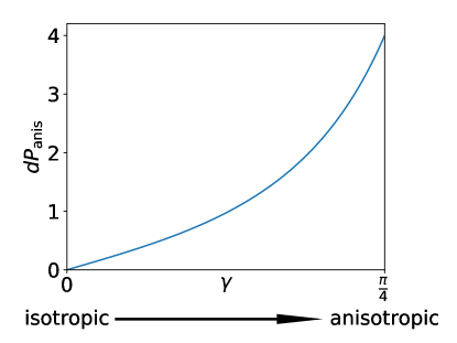
Figure 1: Measure on the initial anisotropy of the Universe as given by (39).

As we can see in Figure 1, the measure slightly favours anisotropic universes over isotropic ones. However, if inflation does occur, it will dilute any initial anisotropy by an exponential amount. Therefore anisotropy will only be observable today if it was initially exponentially large. Such initial conditions represent a tiny fraction of the measure (39), despite the mild enhancement of anisotropic universes. We therefore see that the inclusion of anisotropy has a negligible impact on the results of F18.

Relaxing the assumption of isotropy does not solve the fine tuning issues observed in F18. In the manifold of all possible initial conditions for a single scalar field in a Bianchi I universe, the set that allows $N>60$ e-foldings of inflation represents only a tiny fraction. It is therefore far from clear that inflation truly solves the fine-tuning puzzles that it was designed for.
The author would like to thank Sotirios Karamitsos, Apostolos Pilaftsis and David Sloan for useful comments and discussion. KF is supported by the University of Manchester through the President’s Doctoral Scholar Award.

References

- (1) Alan H. Guth. The Inflationary Universe: A Possible Solution to the Horizon and Flatness Problems. Phys. Rev., D23:347–356, 1981. [Adv. Ser. Astrophys. Cosmol.3,139(1987)].
- (2) Andrei D. Linde. A New Inflationary Universe Scenario: A Possible Solution of the Horizon, Flatness, Homogeneity, Isotropy and Primordial Monopole Problems. Phys. Lett., 108B:389–393, 1982. [Adv. Ser. Astrophys. Cosmol.3,149(1987)].
- (3) Andreas Albrecht and Paul J. Steinhardt. Cosmology for Grand Unified Theories with Radiatively Induced Symmetry Breaking. Phys. Rev. Lett., 48:1220–1223, 1982. [Adv. Ser. Astrophys. Cosmol.3,158(1987)].
- (4) Andrei D. Linde. Initial Conditions for Infaltion. Phys. Lett., 162B:281–286, 1985.
- (5) P. Chmielowski and Don N. Page. Probability of Bianchi Type I Inflation. Phys. Rev., D38:2392–2398, 1988.
- (6) Andrei D. Linde and Arthur Mezhlumian. Stationary universe. Phys. Lett., B307:25–33, 1993.
- (7) Andrei D. Linde, Dmitri A. Linde, and Arthur Mezhlumian. From the Big Bang theory to the theory of a stationary universe. Phys. Rev., D49:1783–1826, 1994.
- (8) Juan Garcia-Bellido, Andrei D. Linde, and Dmitri A. Linde. Fluctuations of the gravitational constant in the inflationary Brans-Dicke cosmology. Phys. Rev., D50:730–750, 1994.
- (9) D. H. Coule. Canonical measure and the flatness of a FRW universe. Class. Quant. Grav., 12:455–470, 1995.
- (10) H. T. Cho and R. Kantowski. A Measure on a subspace of FRW solutions and the flatness problem of standard cosmology. Phys. Rev., D50:6144–6149, 1994.
- (11) W. R. Stoeger, G. F. R. Ellis, and U. Kirchner. Multiverses and cosmology: Philosophical issues. 2004.
- (12) Jaume Garriga, Delia Schwartz-Perlov, Alexander Vilenkin, and Sergei Winitzki. Probabilities in the inflationary multiverse. JCAP, 0601:017, 2006.
- (13) Don N. Page. Predictions and tests of multiverse theories. pages 411–429, 2006.
- (14) Anthony Aguirre, Steven Gratton, and Matthew C Johnson. Measures on transitions for cosmology in the landscape. Phys. Rev. Lett., 98:131301, 2007.
- (15) Anthony Aguirre, Steven Gratton, and Matthew C Johnson. Hurdles for recent measures in eternal inflation. Phys. Rev., D75:123501, 2007.
- (16) Timothy Clifton, Stephen Shenker, and Navin Sivanandam. Volume Weighted Measures of Eternal Inflation in the Bousso-Polchinski Landscape. JHEP, 09:034, 2007.
- (17) Sergei Winitzki. A Volume-weighted measure for eternal inflation. Phys. Rev., D78:043501, 2008.
- (18) Anna Ijjas, Paul J. Steinhardt, and Abraham Loeb. Inflationary paradigm in trouble after Planck2013. Phys. Lett., B723:261–266, 2013.
- (19) Alan H. Guth, David I. Kaiser, and Yasunori Nomura. Inflationary paradigm after Planck 2013. Phys. Lett., B733:112–119, 2014.
- (20) Alejandro Corichi and David Sloan. Inflationary Attractors and their Measures. Class. Quant. Grav., 31:062001, 2014.
- (21) Matthew Kleban and Leonardo Senatore. Inhomogeneous Anisotropic Cosmology. JCAP, 1610(10):022, 2016.
- (22) Katy Clough, Eugene A. Lim, Brandon S. DiNunno, Willy Fischler, Raphael Flauger, and Sonia Paban. Robustness of Inflation to Inhomogeneous Initial Conditions. JCAP, 1709(09):025, 2017.
- (23) Katy Clough, Raphael Flauger, and Eugene A. Lim. Robustness of Inflation to Large Tensor Perturbations. JCAP, 1805(05):065, 2018.
- (24) Josu C. Aurrekoetxea, Katy Clough, Raphael Flauger, and Eugene A. Lim. The Effects of Potential Shape on Inhomogenous Inflation. 2019.
- (25) G. W. Gibbons, S. W. Hawking, and J. M. Stewart. A Natural Measure on the Set of All Universes. Nucl. Phys., B281:736, 1987.
- (26) Dalia S. Goldwirth and Tsvi Piran. Initial conditions for inflation. Phys. Rept., 214:223–291, 1992.
- (27) William E. East, Matthew Kleban, Andrei Linde, and Leonardo Senatore. Beginning inflation in an inhomogeneous universe. JCAP, 1609(09):010, 2016.
- (28) Andrei Linde. On the problem of initial conditions for inflation. Found. Phys., 48(10):1246–1260, 2018.
- (29) R. Penrose. Difficulties with inflationary cosmology. Annals N. Y. Acad. Sci., 571:249–264, 1989.
- (30) G. W. Gibbons and Neil Turok. The Measure Problem in Cosmology. Phys. Rev., D77:063516, 2008.
- (31) Anna Ijjas, Paul J. Steinhardt, and Abraham Loeb. Inflationary schism. Phys. Lett., B736:142–146, 2014.
- (32) Lasha Berezhiani and Mark Trodden. How Likely are Constituent Quanta to Initiate Inflation? Phys. Lett., B749:425–430, 2015.
- (33) S. W. Hawking and Don N. Page. How probable is inflation? Nucl. Phys., B298:789–809, 1988.
- (34) David Sloan and Joseph Silk. Volume Weighting the Measure of the Universe from Classical Slow-Roll Expansion. Phys. Rev., D93(10):104030, 2016.
- (35) Kieran Finn and Sotirios Karamitsos. Finite measure for the initial conditions of inflation. Phys. Rev., D99(6):063515, 2019. [Erratum: Phys. Rev.D99,no.10,109901(2019)].
- (36) Luther Pfahler Eisenhart. Dynamical trajectories and geodesics. Annals of Mathematics, 30(1/4):591–606, 1928.
- (37) Kieran Finn, Sotirios Karamitsos, and Apostolos Pilaftsis. Eisenhart lift for field theories. Phys. Rev., D98(1):016015, 2018.
- (38) Luigi Bianchi. On the three-dimensional spaces which admit a continuous group of motions. Memorie di Matematica e di Fisica della Società Italiana delle Scienze, 11:267–352, Jan 1898.
- (39) C. B. Collins and S. W. Hawking. Why is the Universe isotropic? Astrophys. J., 180:317–334, 1973.
- (40) Ian Moss and Varun Sahni. Anisotropy in the Chaotic Inflationary Universe. Phys. Lett., B178:159–162, 1986.
- (41) John D. Barrow and O. Gron. Homogenization and Isotropization of an Inflationary Cosmological Model. Phys. Lett., B182:25–27, 1986.
- (42) Shigeo Sasaki. On the differential geometry of tangent bundles of Riemannian manifolds. Tohoku Math. J., (2) 10:338–354, 1958.
- (43) J. Liouville. Note sur la théorie de la variation des constantes arbitraires. Journal de Mathématiques Pures et Appliquées, pages 342–349, 1838.
- (44) C. G. J. Jacobi. De formatione et proprietatibus Determinantium. J. Reine Angew. Math., 22:285–318, 1841. [Ostwald’s Klass. Exakt. Wiss.77,3(1896)].
- (45) P.S. Laplace. A philosophical essay on probabilities. Dover books on science. Dover Publications, 1952.