Thin-Shell Wormhole Satisfying Energy Conditions

Abstract

The quartic self-interacting conformal scalar field is used to construct a thin-shell wormhole satisfying all energy conditions. Accompanying the scalar field is the extremal Reissner-Nordström black hole with a positive cosmological constant. New junction conditions apt for the higher-order terms are introduced in the Gaussian normal coordinates. Our approach may provide a guideline towards getting rid of exotic matter in TSWs.

I Introduction

Black holes with the hair of conformal scalar field entered into physics literature with the Einstein-Maxwell-Scalar (EMS) solutions, given by Bochorova, Bronikov and Melnikov (Bocharova1, ), and later independently by Bekenstein (Bekenstein1, ). These works will be referred together as BBMB. In obtaining this solution, the extremal Reissner-Nordström (ERN) solution was used as base on which the scalar field was added. The scalar field itself turned out to be singular at the horizon whereas the spacetime was regular, as it should be. The interest in such a solution was due to the fact that a test scalar field, in contrast to the coupled scalar field, did not feel the singularity so that the physics went normal at the horizon. Conformal scalar field is important because it is related to the scaling of spacetime coordinates. The history of such scaling, in connection with scalar fields and their use in field theory, goes back to the idea of Lifshitz . The spinless scalar interaction between objects naturally provides the simplest type of interaction in both classical and quantum field theory. Global scaling of coordinates may be valid in a spacetime leading to certain conserved quantities. More importantly, the local scaling which amounts to $g_{\mu\nu}\rightarrow\varOmega^{2}g_{\mu\nu}$, and scalar field $\psi\rightarrow\varOmega^{-1}\psi$, change the equation satisfied by the scalar field $\psi$, so that the revised version becomes of the form $\nabla^{2}\psi-\frac{1}{6}R\psi=0$, involving the scalar curvature of the spacetime. Further extensions with conformal scalar of black hole solutions follow by taking into account the higher order coupling of scalar fields higher than the quadratic ones. One such solution with a positive cosmological constant and conformal scalar fields was given by Martínez, Troncoso and Zanelli (MTZ solution) (Martinez1, ). Their solution was also built on the ERN solution with positive cosmological constant, and a static electric charge. However, as the BBMB solution introduced a new scalar hair, the MTZ solution did not do so. It happens that the scalar hair is expressed in terms of mass and charge. Furthermore, the scalar field diverges on the event horizon as in the case of BBMB. Yet, the latter is an interesting black hole solution covering a positive cosmological constant, electric charge and a conformal scalar field of fourth order. An interesting property of MTZ is that it satisfies the energy conditions such as the strong and the dominant energy conditions (SEC and DEC). This latter property attracted our interest and motivated us to construct a thin-shell wormhole (TSW) that may satisfy physical energy conditions without need of exotic matter. From this token, we adopt the model of MTZ with minor rearrangements and apply the method of TSW developed by Visser (Visser1, ). Our primary task toward this goal is to derive new junction conditions in this new theory of gravity. It is well-known that in Einstein’s general relativity such junction conditions were developed first by Israel (Israel1, ). For new coupling terms in the Lagrangian, it is crucial that new junction conditions are used. Previously, new junction conditions have been developed for different theories (Davis1, ; Reina1, ; Senovilla, ) and in the same line of thought we do the same in the present theory. We employ the Gaussian normal coordinate system and find the extrinsic curvature within the set of Gauss-Codazzi equations. Although the equations are tedious, we impose the conditions that upon crossing the thin-shell metric functions are continuous while their normal derivatives may admit discontinuity. We recall that these adopted conditions are the standard ones used in physics in general. Upon this approach, all equations on the surface reduce to simple conditions that the problem becomes tractable enough to construct TSWs. The physical finding is that above certain range of parameters such TSW admits physically satisfactory energy conditions. As a result of considering a quartic coupling term for a conformal scalar field with ERN and positive cosmological constant, we construct a physical TSW, free of exotic matter. Further models can be employed with new and higher order couplings, provided the junction conditions are developed separately in each case.

The order of the letter is as the following. In section II we have developed the junction conditions apt for the gravity theory considered here. In section III we construct a symmetric TSW and study the situations under which the TSW satisfies the known energy conditions. Finally, we conclude in section IV.

II Junction Conditions

The action for a conformal massless scalar field $\psi$ coupled to the cosmological Einstein-Hilbert density and other fields $\mathcal{L}_{M}$ is given by (Martinez1, )

$$I=\frac{1}{2\kappa}\int\sqrt{-g}d^{4}x\left[R-2\Lambda\left(1-\alpha^{2}\psi^{4}\right)\right.\\ \left.-\alpha\left(\psi^{2}R+6\partial_{\mu}\psi\partial^{\mu}\psi\right)+2\kappa\mathcal{L}_{M}\right],$$ (1)

in which $\kappa=8\pi G/c^{4}$ is the Einstein constant, $\Lambda$ is the cosmological constant, and $\alpha$ is a coupling constant. Here we choose $c=1$ by convention. To obtain MTZ solution (Martinez1, ), the existence of the quartic interaction term to the cosmological expression is inevitable. It is also noteworthy to point out that the above Lagrangian density (without the matter field) is in fact a special case of Horndeski theory (Horndeski1, ) with $K\left(\psi,X\right)=\left(1/\kappa\right)\left[6\alpha X-\Lambda\left(1-\alpha^{2}\psi^{4}\right)\right]$, $G_{4}\left(\psi,X\right)=\left(1/2\kappa\right)\left(1-\alpha\psi^{2}\right)$, and $G_{3}\left(\psi,X\right)=G_{5}\left(\psi,X\right)=0$ (Ganguly1, ). Varying this action with respect to the scalar field $\psi$ leads to the conformal equation

$$\nabla^{2}\psi-\frac{1}{6}\psi R+\frac{2}{3}\alpha\Lambda\psi^{3}=0,$$ (2)

whereas variation with respect to the metric tensor $g_{\mu\nu}$ yields the field equation

$$G_{\mu\nu}\left(1-\alpha\psi^{2}\right)+\Lambda g_{\mu\nu}\left(1-\alpha^{2}\psi^{4}\right)=\\ \left[6\alpha\partial_{\mu}\psi\partial_{\nu}\psi-3\alpha\left(\partial\psi\right)^{2}g_{\mu\nu}\right.\\ \left.-\alpha\nabla_{\mu}\nabla_{\nu}\left(\psi^{2}\right)+\alpha\nabla^{2}\left(\psi^{2}\right)g_{\mu\nu}+\kappa T_{\mu\nu}\right],$$ (3)

in which $G_{\mu\nu}=R_{\mu\nu}-\frac{1}{2}Rg_{\mu\nu}$ is the Einstein tensor and $T_{\mu\nu}$ is the energy-momentum tensor due to the existing sources. Actually, the name conformal scalar field is due to the fact that Eq. (2) is invariant under the conformal transformation $g_{\mu\nu}\rightarrow\varOmega^{2}g_{\mu\nu}$ and $\psi\rightarrow\varOmega^{-1}\psi$, where $\varOmega$ is an arbitrary differentiable function. However, since the Einstein-Hilbert term is not invariant under such a transformation, the action in whole is not conformal. By contracting Eq. (3) and utilizing Eq. (2), one can easily show that

$$R=4\Lambda-\kappa T,$$ (4)

which implies $R=4\Lambda=const.$ for a cosmological action without a matter field, or a trace-free energy-momentum tensor (such as the one of the electromagnetic field). Simultaneous consideration of Eqs. (2), (3), and (4) leads to an alternative form for Eq. (3), i.e.

$$\left[R_{\mu\nu}-\Lambda g_{\mu\nu}\left(1+\frac{1}{3}\alpha^{2}\psi^{4}\right)\right]\left(1-\alpha\psi^{2}\right)+\alpha\Upsilon_{\mu\nu}\\ =\kappa\left[T_{\mu\nu}-\frac{1}{2}T\left(1-\frac{1}{3}\alpha\psi^{2}\right)g_{\mu\nu}\right],$$ (5)

where we have defined

$$\Upsilon_{\mu\nu}=\nabla_{\mu}\nabla_{\nu}\left(\psi^{2}\right)+\left(\partial\psi\right)^{2}g_{\mu\nu}-6\partial_{\mu}\psi\partial_{\nu}\psi.$$ (6)

The Gauss-Codazzi equations for Ricci tensor elements in Gaussian normal coordinates are given by

$$R_{wa}=-\nabla_{a}K+\nabla_{b}K_{a}^{b},$$ (7)

$$R_{ab}=\,^{\mathcal{H}}R_{ab}-\partial_{w}K_{ab}+2K_{a}^{c}K_{cb}-KK_{ab},$$ (8)

$$R_{ww}=-g^{ab}\partial_{w}K_{ab}+Tr\left(K^{2}\right),$$ (9)

for an $n$-dimensional hypersurface embedded in an $n+1$-dimensional bulk spacetime. In this framework, $w$ is the spatial Gaussian normal coordinate and the timelike hypersurface exists at $w=0$, so the metric of the hypersurface could be depicted as

$$ds_{\mathcal{H}}^{2}=dw^{2}+g_{ab}dx^{a}dx^{b}.$$ (10)

Furthermore, $\,{}^{\mathcal{H}}R_{ab}$ is the induced Ricci tensor on the hypersurface, $K_{ab}\equiv\frac{1}{2}\partial_{w}g_{ab}$ and $K\equiv g^{ab}K_{ab}$ are the extrinsic curvature tensor and the total curvature, respectively, and $Tr\left(K^{2}\right)\equiv K^{ab}K_{ab}$. Upon direct substitution of the three Gauss-Codazzi equations into Eq. (5) with appropriate indices, after some mathematical manipulation one could recover

$$\left(\nabla_{a}K-\nabla_{b}K_{a}^{b}\right)\left(1-\alpha\psi^{2}\right)\\ +\alpha\left[\partial_{w}\partial_{a}\left(\psi^{2}\right)-\varGamma_{wa}^{\mu}\partial_{\mu}\left(\psi^{2}\right)-6\partial_{w}\left(\psi\right)\partial_{a}\left(\psi\right)\right]=\\ \kappa\left\{T_{iw}^{+}\varTheta\left(w\right)+T_{iw}^{-}\varTheta\left(-w\right)\right\},$$ (11)

$$\left[\,{}^{\mathcal{H}}R_{ab}-\partial_{w}K_{ab}+2K_{a}^{c}K_{cb}-KK_{ab}\right.\\ \left.-\Lambda g_{ab}\left(1+\frac{1}{3}\alpha^{2}\psi^{4}\right)\right]\left(1-\alpha\psi^{2}\right)\\ +\alpha\left[\partial_{a}\partial_{b}\left(\psi^{2}\right)-\varGamma_{ab}^{\mu}\partial_{\mu}\left(\psi^{2}\right)-6\partial_{a}\left(\psi\right)\partial_{b}\left(\psi\right)+\left(\partial\psi\right)^{2}g_{ab}\right]=\\ \kappa\left\{T_{ab}^{+}\varTheta\left(w\right)+T_{ab}^{-}\varTheta\left(-w\right)+S_{ab}\delta\left(w\right)\right.\\ \left.-\frac{1}{2}g_{ab}\left[T^{+}\varTheta\left(w\right)+T^{-}\varTheta\left(-w\right)+S\delta\left(w\right)\right]\left(1-\frac{1}{3}\alpha\psi^{2}\right)\right\},$$ (12)

and

$$\left[-g^{ab}\partial_{w}K_{ab}+Tr\left(K^{2}\right)-\Lambda\left(1+\frac{1}{3}\alpha^{2}\psi^{4}\right)\right]\left(1-\alpha\psi^{2}\right)\\ +\alpha\left[\partial_{w}^{2}\left(\psi^{2}\right)-6\left(\partial_{w}\psi\right)^{2}+\left(\partial\psi\right)^{2}\right]=\\ \kappa\left\{T_{ww}^{+}\varTheta\left(w\right)+T_{ww}^{-}\varTheta\left(-w\right)\right.\\ \left.-\frac{1}{2}\left[T^{+}\varTheta\left(w\right)+T^{-}\varTheta\left(-w\right)+S\delta\left(w\right)\right]\left(1-\frac{1}{3}\alpha\psi^{2}\right)\right\}$$ (13)

corresponding to Eqs. (7), (8), and (9), respectively. In these latter equations, we have used the fact that in the immediate neighborhood of the hypersurface, the energy-momentum tensor of the bulk spacetime and of the hypersurface itself could collectively be written as

$$T_{\mu\nu}=T_{\mu\nu}^{+}\varTheta\left(w\right)+T_{\mu\nu}^{-}\varTheta\left(-w\right)+S_{\mu\nu}\delta\left(w\right),$$ (14)

where $\varTheta$ and $\delta$ denote the Heaviside step function and the Dirac delta function, respectively, while $S_{\mu\nu}$ is the induced energy-momentum tensor on the hypersurface. Furthermore, note that according to the selection of the Gaussian normal coordinates, we have $g_{wa}=0$, $g_{ww}=1$ and $S_{wa}=S_{ww}=0$, identically.

Taking integral of Eqs. (11), (12) and (13) over a volume in the neighborhood around the hypersurface from $-\epsilon$ to $\epsilon$, and then operating a limit at which $\epsilon\rightarrow 0$, lead us to the boundary conditions we are looking for. In what follows we assume that $\psi$ is a continuous function across the hypersurface. This assumption is somehow necessary in order to avoid the emergence of mathematically non-acceptable expressions such as a multiplication of two Dirac delta functions. Starting from Eq. (11), we observe that the only total integrand is $\partial_{w}\partial_{a}\left(\psi^{2}\right)$, which makes it the only term that survives the limiting process. In other words, operating $\underset{\epsilon\rightarrow 0}{\lim}\intop_{-\epsilon}^{\epsilon}dw$ on $\eqref{eq:11}$ yields

$$\underset{\epsilon\rightarrow 0}{\lim}\intop_{-\epsilon}^{\epsilon}\alpha\left[\partial_{w}\partial_{a}\left(\psi^{2}\right)\right]dw=\underset{\epsilon\rightarrow 0}{\lim}\alpha\left[\partial_{a}\left(\psi^{2}\right)\right]_{-\epsilon}^{\epsilon}=0,$$ (15)

which immediately reduces to

$$\left[\partial_{a}\left(\psi\right)\right]_{-}^{+}=0.$$ (16)

In the latter equation, $\left[\,\right]_{-}^{+}$ denotes a jump in the included term across the hypersurface , i.e. $\left[\partial_{a}\left(\psi\right)\right]_{-}^{+}=\left.\partial_{a}\left(\psi\right)\right|_{+0}-\left.\partial_{a}\left(\psi\right)\right|_{-0}$. This means that not only $\psi$, but also its first tangential derivatives are continuous across the hypersurface. However, if $\psi$ is only a function of the normal coordinate $w$, this condition is self-satisfied. Applying the similar process to Eqs. (12) and (13), and raising one of the indices in the first equation gives rise to

$$\left(1-\alpha\psi^{2}\right)\left[K_{a}^{b}\right]_{-}^{+}=-\kappa\left[S_{a}^{b}-\frac{1}{2}\delta_{a}^{b}S\left(1-\frac{1}{3}\alpha\psi^{2}\right)\right]$$ (17)

and

$$-\left(1-\alpha\psi^{2}\right)\left[K\right]_{-}^{+}+\alpha\left[\partial_{w}\left(\psi^{2}\right)\right]_{-}^{+}=\\ -\kappa\left[\frac{1}{2}S\left(1-\frac{1}{3}\alpha\psi^{2}\right)\right]$$ (18)

respectively. Although Eq. (18) looks to be different from (17), in fact it is not. To show this, it is enough to apply the integration-limiting process to the conformal equation given in Eq. (2) to see that

$$\left[\partial_{w}\left(\psi^{2}\right)\right]_{-}^{+}=-\frac{2}{3}\psi^{2}\left[K\right]_{-}^{+}.$$ (19)

Direct substitution into Eq. (18) simplifies it to

$$\left[K\right]_{-}^{+}=\frac{1}{2}\kappa S,$$ (20)

which is nothing but the trace of Eq. (17). It is not hard to see that for $\alpha\rightarrow 0$ (or $\psi\rightarrow 0$) the original Israel junction conditions are recovered, as expected. The results are in full agreement with Eqs. (3.42) and (3.43) of (Aviles1, ). It is worth-mentioning that all the above calculations were done while we initially had assumed that the first fundamental form (the metric) is continuous across the shell. This rather intuitive condition, which guarantees the smoothness of a hypothetical passage through the shell, is generally accepted as the first junction condition in all thin-shell formalisms.

III Thin-Shell wormhole construction

The above junction conditions, Eqs. (16) and (17) could be used to construct a TSW, provided that we have an exact solution to the action in Eq. (1). Here we consider a de Sitter black hole solution in (Martinez1, ) by MTZ, given with the spherically symmetric line element

$$ds^{2}=-f\left(r\right)dt^{2}+f\left(r\right)^{-1}dr^{2}+r^{2}d\Omega^{2},$$ (21)

with metric function

$$f\left(r\right)=-\left(\frac{r}{l}\right)^{2}+\left(1-\frac{m}{r}\right)^{2},$$ (22)

where $d\Omega^{2}$ is the line element of the unit sphere, $l\equiv\sqrt{3/\Lambda}$ is the cosmological length, and $m$ is the gravitational mass which is related to the scalar field through

$$\psi\left(r\right)=\frac{\alpha^{-1/2}m}{r-m}.$$ (23)

The solution is given only for a positive cosmological constant and in general has an inner, an event, and a cosmological horizon at

$$r_{i}=\frac{l}{2}\left(-1+\sqrt{1+4m/l}\right),$$ (24)

$$r_{e}=\frac{l}{2}\left(1-\sqrt{1-4m/l}\right),$$ (25)

and

$$r_{c}=\frac{l}{2}\left(1+\sqrt{1-4m/l}\right),$$ (26)

respectively. Depending on the values of the mass $m$ and the cosmological length $l$, the solution may exhibit all three, two or only one horizon. For $m=0$ there is only a single cosmological horizon at $r_{c}=l$. For $0<m/l<1/4$ all three horizons are real. For $m=l/4$ the event and the cosmological horizons, $r_{e}$ and $r_{c}$, coincide and hence we have only two horizons. Nonetheless, for $m>l/4$ the solution turns into non-black hole for which the inner horizon changes role to a new cosmological horizon. This last situation is interesting, as will be seen in the following lines. It is also evident that in the limit $\Lambda\rightarrow 0$ ($l\rightarrow\infty$) the action in Eq. (1) and the metric function in Eq. (22) coalesce with the action considered and the solution given by Bocharova, Bronnikov and Melnikov in (Bocharova1, ) and Bekenstein in (Bekenstein1, ), separately, today known as the BBMB solution. Note that the structure of the metric function in Eq. (22) is de Sitter – extremal Reissner–Nordström, whose corresponding TSW has already been studied in pure Einstein gravity (Eid1, ).

To construct the TSW, we follow Visser’s cut-and-paste recipe (Visser1, ). By cutting two exact exterior copies from the MTZ spacetime such that the cutting radius $a$ is greater than (any possible) event horizon and less than the cosmological horizon, we bring them together at their common timelike hypersurface $\mathcal{H}\coloneqq r_{\pm}-a=0$, which is now identified as the throat of the wormhole. Note that the TSW in this fashion will be symmetric. An asymmetric TSW (Forghani1, ), however, could be constructed by specifying different cosmological constants to the two sides, i.e. $\Lambda_{+}\neq\Lambda_{-}$. Nonetheless, this could not be done by considering different masses for the two sides since the mass is coupled to the scalar field via Eq. (23) and earlier in the derivation of the junction conditions we required $\psi\left(r\right)$ to be a continuous function across the shell. Therefore, $\left.\psi_{+}\right|_{r_{+}=a}=\left.\psi_{-}\right|_{r_{-}=a}$ necessarily results in $m_{+}=m_{-}$.

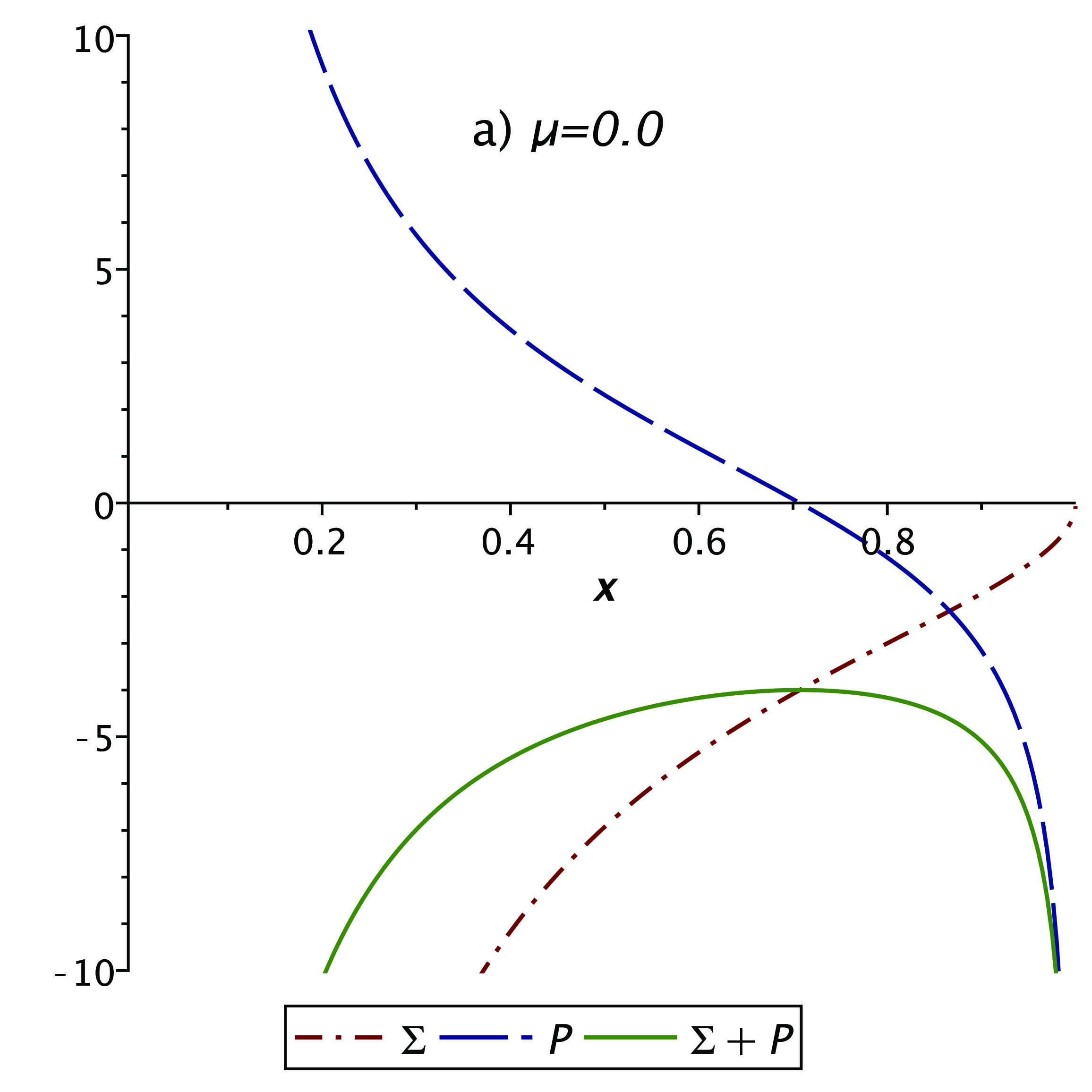
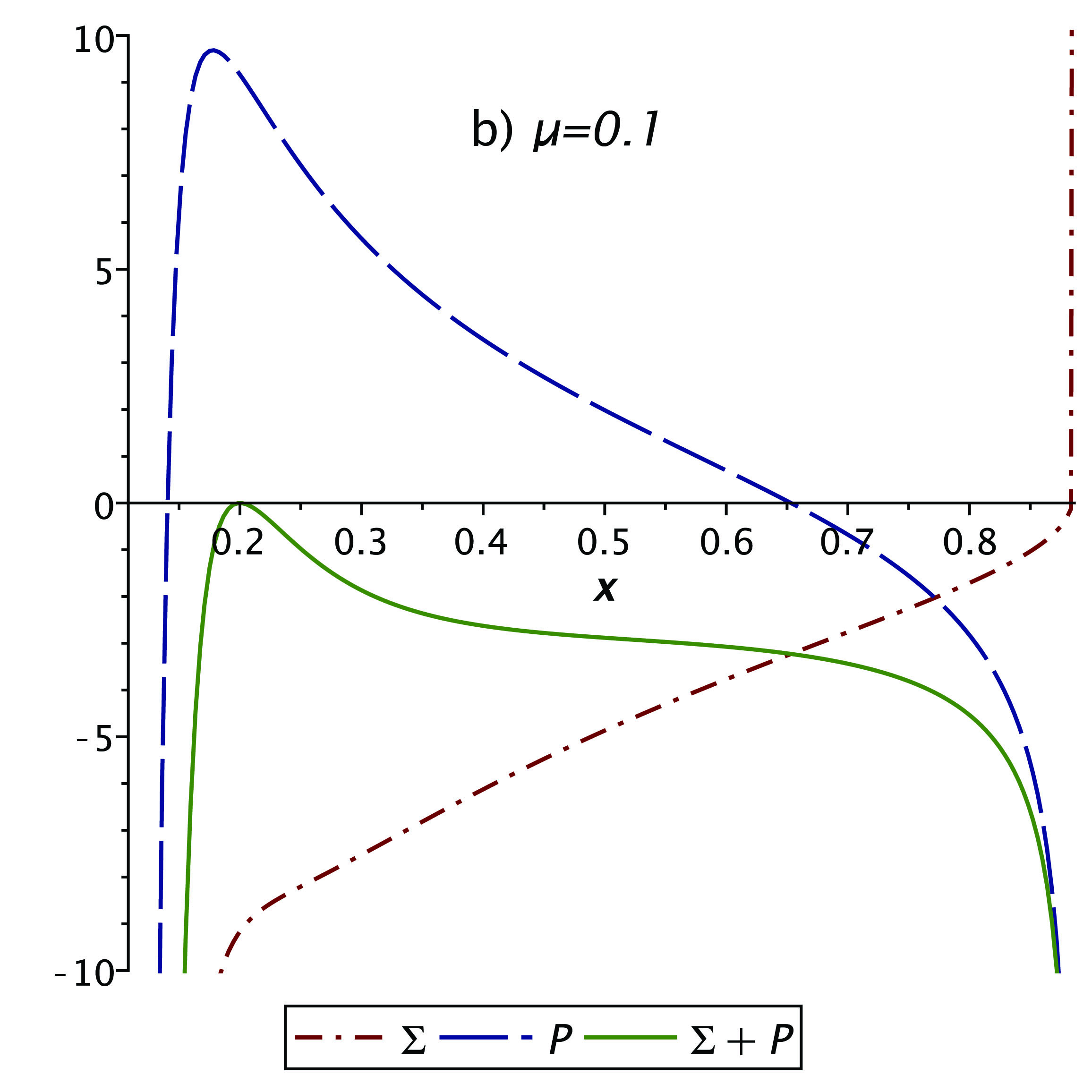
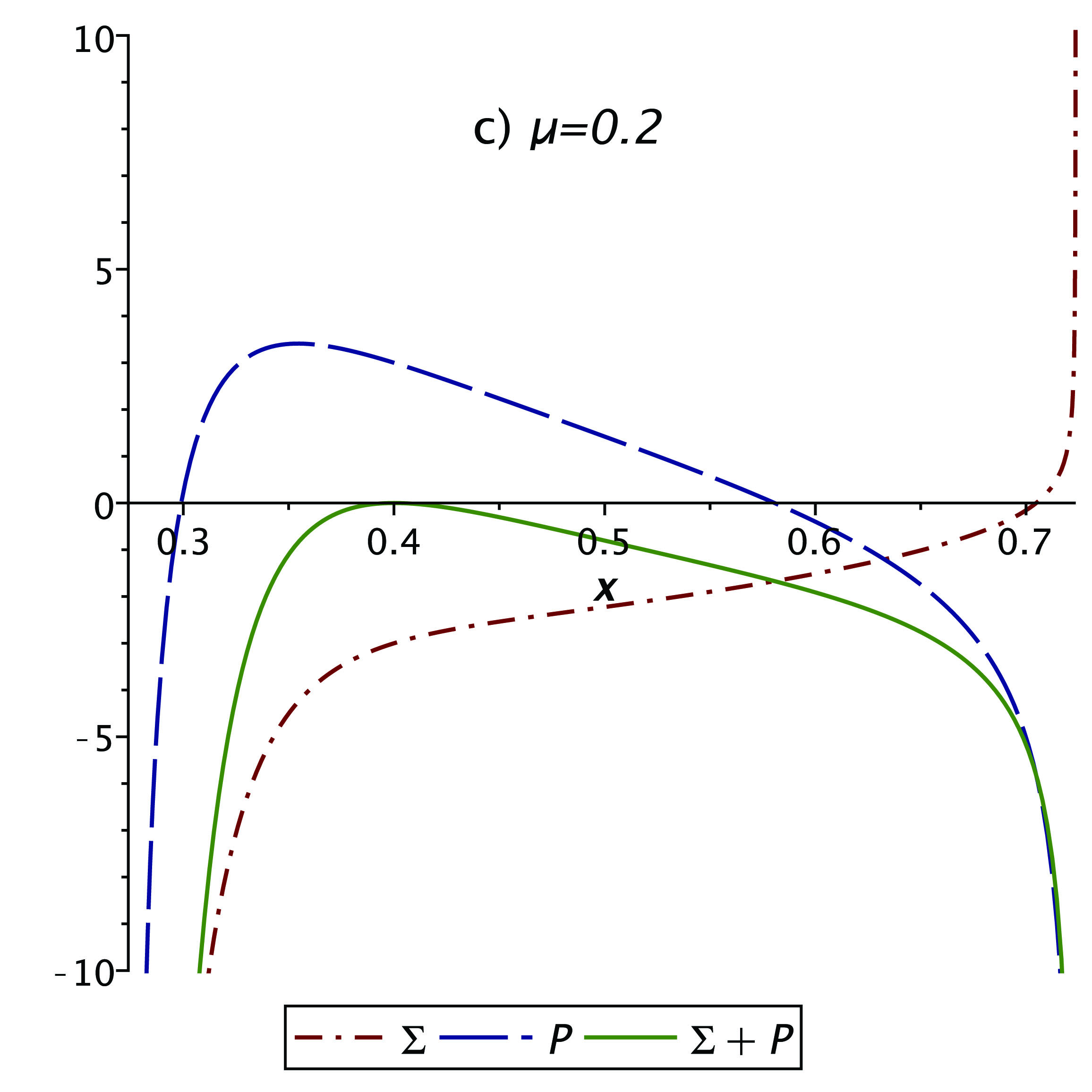
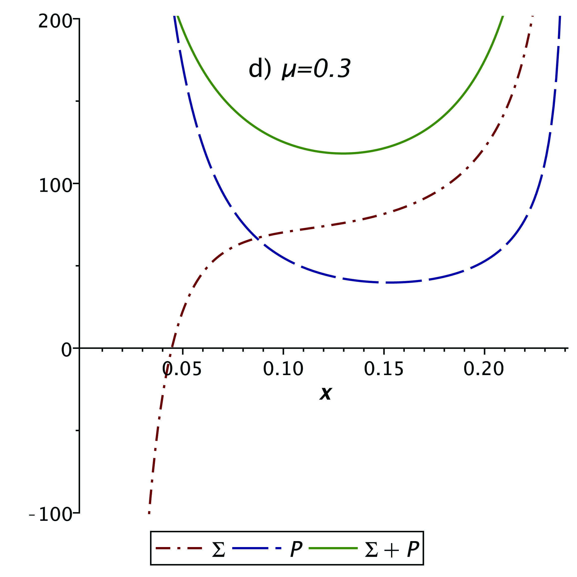
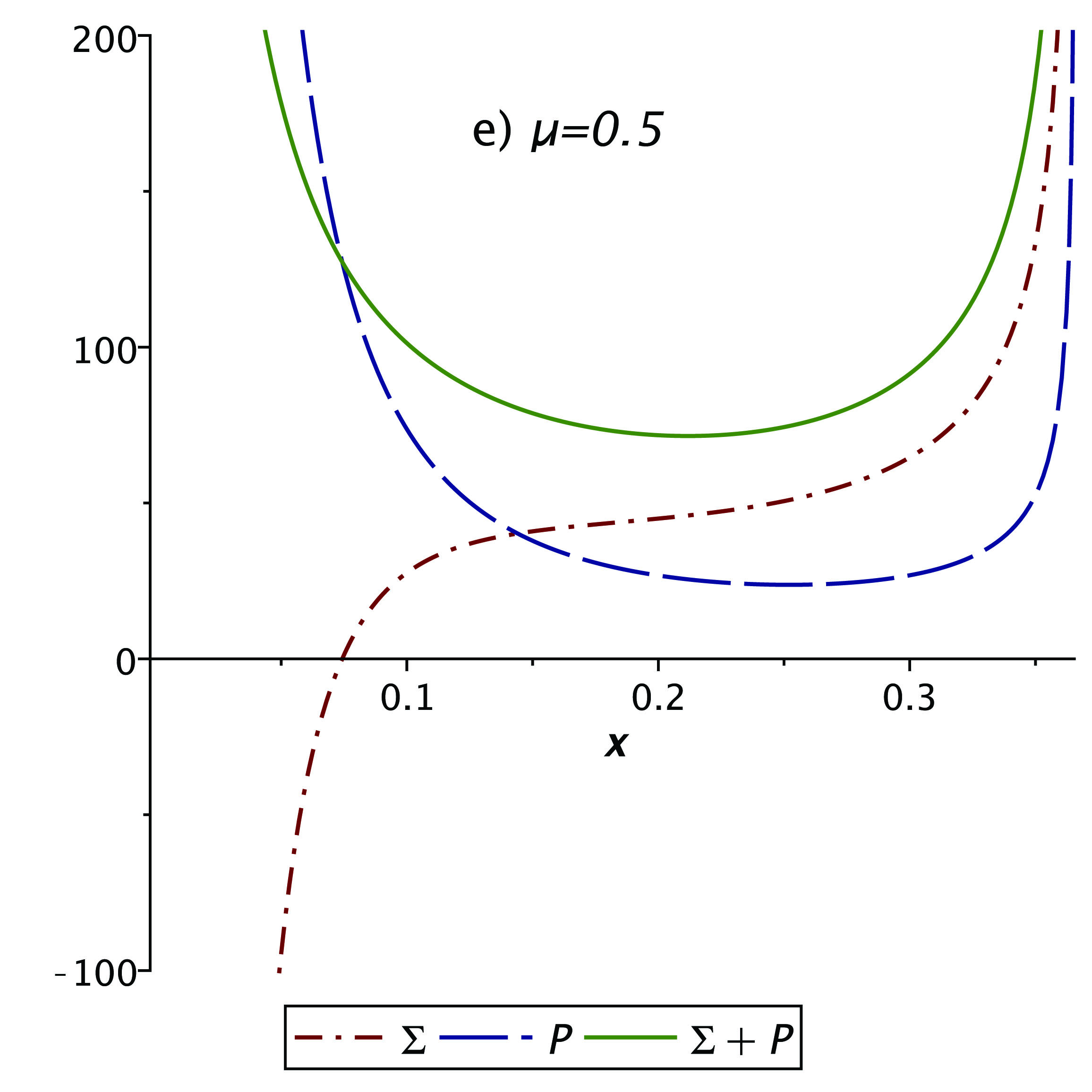
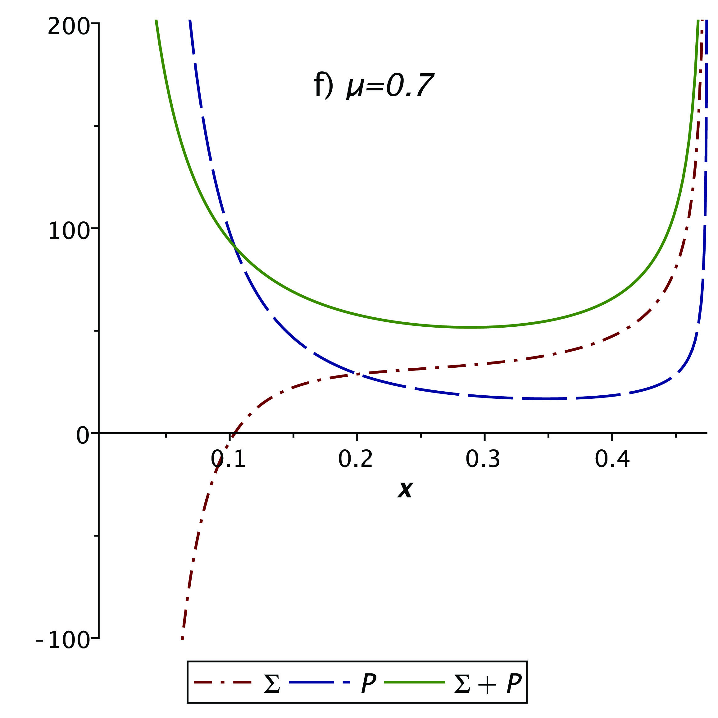
Figure 1: The diagram of the rescaled energy density, $\Sigma\equiv\kappa l\sigma$, the rescaled pressure $P\equiv\kappa lp$ and their summation $\Sigma+P$, against the rescaled radius $x\equiv r/l$ for six values of the mass ratio $\mu\equiv m/l$.

With this symmetric configuration, we will be looking for conditions under which the TSW could exist without relying on any exotic matter. The question whether such construction is stable against a radial perturbation or not will be postponed to future researches. The first junction condition requires a unique metric for the thin-shell, no matter which spacetime it is approached from. Therefore, we will have

$$ds_{\mathcal{H}}^{2}=-d\tau^{2}+a^{2}d\Omega^{2}$$ (27)

on the shell (on the throat), where $\tau$ and $a$ are the proper time and the radial coordinate of the shell, respectively. The second junction condition, given in Eq. (16), is already satisfied since the scalar field is only a function of the radial coordinate (which happens to be the Gaussian normal coordinate in this configuration), not the defining coordinates of the throat. To examine the third junction condition, given in Eq. (17), one needs prior preparations. Firstly, the mixed extrinsic curvature tensor of the two spacetimes must be calculated. Secondly, a certain energy-momentum tensor must be considered. Here we employ the energy-momentum tensor of a perfect fluid which is indicated by

$$S_{a}^{b}=diag(-\sigma,p,p),$$ (28)

where $\sigma$ is the energy density, and $p$ is the angular pressure of the fluid at the throat. To calculate the curvature tensor one might use a rather explicit definition of it, given by

$$K_{ab}^{\pm}=-n_{\gamma}^{\pm}\left(\frac{\partial^{2}x_{\pm}^{\gamma}}{\partial\xi^{a}\partial\xi^{b}}+\Gamma_{\alpha\beta}^{\gamma\pm}\,\frac{\partial x_{\pm}^{\alpha}}{\partial\xi^{a}}\frac{\partial x_{\pm}^{\beta}}{\partial\xi^{b}}\right),$$ (29)

where $x_{\pm}^{\alpha}$ and $\xi^{a}$ are the coordinates of the bulks and of the throat, respectively, while $\Gamma_{\alpha\beta}^{\gamma\pm}$ are the Christoffel symbols compatible with the bulks’ metrics. Furthermore, $n_{\gamma}^{\pm}$ are the components of the $4$-normal to the throat, given by

$$n_{\gamma}^{\pm}=\pm\left|g^{\alpha\beta}\,\frac{\partial\mathcal{H}}{\partial x_{\pm}^{\alpha}}\frac{\partial\mathcal{H}}{\partial x_{\pm}^{\beta}}\right|^{-1/2}\frac{\partial\mathcal{H}}{\partial x_{\pm}^{\gamma}}.$$ (30)

Skipping the details of the calculations, the energy density $\sigma$ and the angular pressure $p$ are found to be

$$\sigma=-\frac{2}{\kappa}\sqrt{f}\left[\left(\frac{1}{3}\alpha\psi^{2}\right)\frac{f^{\prime}}{f}+\left(1-\frac{1}{3}\alpha\psi^{2}\right)\frac{2}{a}\right],$$ (31)

and

$$p=\frac{1}{\kappa}\sqrt{f}\left[\left(1-\frac{1}{3}\alpha\psi^{2}\right)\frac{f^{\prime}}{f}+\left(1+\frac{1}{3}\alpha\psi^{2}\right)\frac{2}{a}\right],$$ (32)

respectively, where a prime (^′) denotes a total derivative with respect to the radial coordinate and all the parameters and functions are evaluated at the throat’s radius. It can be observed that unlike the forms that generally appear in Einstein’s relativity, $\sigma$ is not trivially negative-definite, and hence, there might be a chance for the weak energy condition (WEC) to be satisfied for the matter on the throat. To explore this, we directly substitute the metric function from Eq. (22), and the scalar field from Eq. (23), into Eqs. (31) and (32) to obtain

$$\Sigma=\frac{4\left(3x^{5}-3x^{4}\mu-3x^{3}+9x^{2}\mu-8x\mu^{2}+\mu^{3}\right)}{3\sqrt{-x^{4}+\mu^{2}-2\mu x+x^{2}}\left(x-\mu\right)x^{2}},$$ (33)

and

$$P=\frac{2\left(6x^{4}\mu-6x^{5}-2\mu^{3}+4x\mu^{2}-6x^{2}\mu+3x^{3}\right)}{3\sqrt{-x^{4}+\mu^{2}-2\mu x+x^{2}}x^{2}\left(x-\mu\right)},$$ (34)

as well as

$$\Sigma+P=\frac{-2\left(x-2\mu\right)^{2}}{\sqrt{-x^{4}+\mu^{2}-2\mu x+x^{2}}x\left(x-\mu\right)},$$ (35)

Herein, we have rescaled the mass by $\mu\equiv m/l$, the radius by $x\equiv r/l$, the energy density by $\Sigma\equiv\kappa l\sigma$ and the angular pressure by $P\equiv\kappa lp$. Fig. 1 illustrates the rescaled energy density $\Sigma$, the pressure $P$ and the sum $\Sigma+P$ versus the rescaled radius $x$, for six different values of $\mu$; $0.0$, $0.1$, $0.2$, $0.3$, $0.5$ and $0.7$. The radius of the TSW in Figs. 1a-1c , where $\mu<0.25$ ($m/l<1/4$), falls between the rescaled event horizon $x_{e}\equiv r_{e}/l=\frac{1}{2}\left(1-\sqrt{1-4\mu}\right)$ and the rescaled cosmological horizon $x_{c}\equiv r_{c}/l=\frac{1}{2}\left(1+\sqrt{1-4\mu}\right)$. As it is observed from these figures, for $0<\mu<0.25$ although $\Sigma$ becomes positive for radii in the neighborhood of the cosmological horizon, the sum $\Sigma+P$ is positive nowhere. Therefore, the energy conditions are not satisfied and the matter is exotic. However, once $\mu$ exceeds $0.25$ the permissible universe lies within the rescaled inner radius $x_{i}\equiv r_{i}/l=\frac{1}{2}\left(-1+\sqrt{1+4\mu}\right)$, which now is the cosmological horizon of this universe. In Figs. 1d-1f, $\Sigma$ and $P$ have simultaneously become positive for a wide domain of admissible $x$; and so does $\Sigma+P$. This emphasizes that, not only the weak energy condition (WEC), but also the dominant energy condition (DEC) given by $\Sigma>\left|P\right|$, and the strong energy condition (SEC), given by $\Sigma+P>0$ and $\Sigma+3P>0$, are satisfied, so the TSW is supported by ordinary matter instead of exotic.

IV Conclusion

For a long time exotic matter violating the energy conditions has been an indispensable source for the survival of a TSW. In search for a remedy to this long-standing problem, we resort to new physical systems that involve new coupling terms. In this study we employed a black hole solution that involves, in addition to the ERN, a positive cosmological constant and a self-interacting conformal scalar field of fourth order. With these new terms, the standard junction conditions of general relativity for thin-shells must be modified. Accordingly, we derived the revised form of the junction conditions by using the Gauss-Codazzi equations. Upon imposing these new junction conditions, we obtain simple results that are easily tractable. As a result, we established a new TSW that satisfies WEC and DEC without reference to exotic sources. To achieve this, however, the mass and the cosmological radius of the resulting solution must exceed beyond certain minima.

References

- (1) N. Bocharova, K. Bronnikov, and V. Melnikov, Vestn. Mosk. Univ., Fiz., Astron. 6, 706 (1970).
- (2) J. D. Bekenstein, Ann. Phys. (N.Y.) 82, 535 (1974); 91, 75 (1975).
- (3) G.L. Klimchitskaya, U. Mohideen, and V.M. Mostepanenko, Rev. Modern Phys. 81, 1827 (2009).
- (4) M. Visser, Phys. Rev. D 39, 3182 (1989); Nucl. Phys. B 328, 203 (1989).
- (5) W. Israel, Nuovo Cim. B 44S10, 1 (1966); Erratum ibid. B 48, 463 (1967).
- (6) S.C. Davis, Phys. Rev. D 67, 024030 (2003).
- (7) J.M.M. Senovilla, Phys. Rev. D 88, 064015 (2013).
- (8) B. Reina, J.M.M. Senovilla, R. Vera, Class. Quantum Gravity 33, 105008 (2016).
- (9) C. Martínez, R. Troncoso, and J. Zanelli, Phys. Rev. D 67, 024008 (2003).
- (10) G.W. Horndeski, Int. J. Theor. Phys. 10, 363 (1974).
- (11) A. Ganguly, R. Gannouji, M. Gonzalez-Espinoza, and C. Pizarro-Moya, Class. Quantum Grav. 35, 145008 (2018).
- (12) L. Avilés, H. Maeda, and C. Martinez, arXiv:1910.07534.
- (13) A. Eid, New Astron. 39, 72 (2015).
- (14) S.D. Forghani, S.H. Mazharimousavi, and M. Halilsoy, Eur. Phys. J. C 78, 469 (2018); J. Cosmol. Astropart. Phys. 10, 067 (2019).